Embed Size (px)
Citation preview
Introduction to R
Le YanHPC User Services @ LSU
3/2/2016 HPC training series Spring 2016
Some materials are borrowed from the “Data Science” course by John Hopkins University on Coursera.
Outline
• R basics– Getting started– Data classes and objects
• Data analysis case study: NOAA weather hazard data
3/2/2016 HPC training series Spring 2016 1
The History of R• R is a dialect of the S language
– S was initiated at the Bell Labs as an internal statistical analysis environment
– Most well known implementation is S‐plus (most recent stable release was in 2010)
• R was first announced in 1993• The R core group was formed in 1997, who controls the
source code of R (written in C)• R 1.0.0 was released in 2000• The current version is 3.2.3
3/2/2016 HPC training series Spring 2016 2
Features of R• R is a dialect of the S language
– Language designed for statistical analysis– Similar syntax
• Available on most platform/OS• Rich data analysis functionalities and sophisticated graphical
capabilities• Active development and very active community
– CRAN: The Comprehensive R Archive Network• Source code and binaries, user contributed packages and documentation
– More than 6,000 packages available on CRAN (as of March 2015)• Free to use
3/2/2016 HPC training series Spring 2016 3
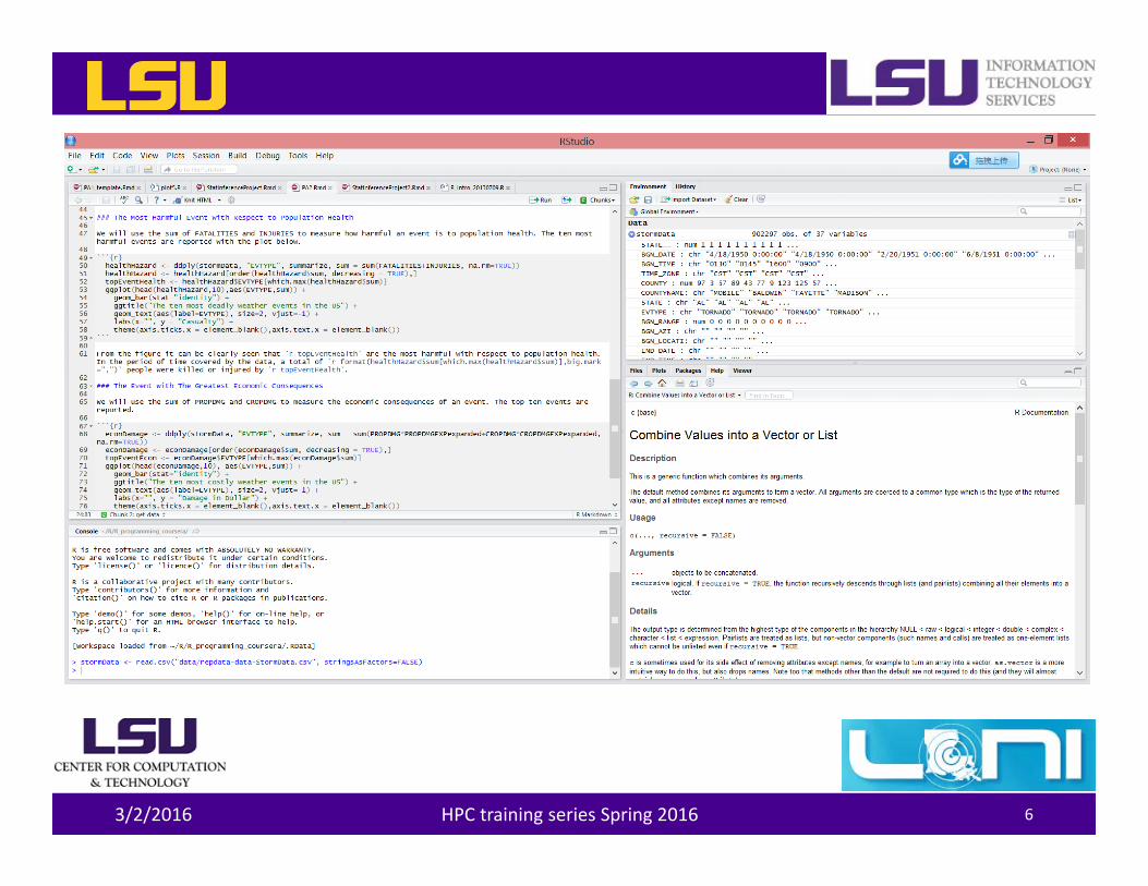
Two Ways of Running R• With an IDE
– Rstudio is the de facto environment for R on a desktop system
• On a cluster– R is installed on all LONI and LSU HPC clusters
• QB2: r/3.1.0/INTEL-14.0.2• SuperMIC: r/3.1.0/INTEL-14.0.2• Philip: r/3.1.3/INTEL-15.0.3• SuperMike2: +R-3.2.0-gcc-4.7.2
3/2/2016 HPC training series Spring 2016 4
Rstudio• Free to use• Similar user interface to other, dividing the screen into
panes– Source code– Console– Workspace– Others (help message, plot etc.)
• Rstudio in a desktop environment is better suited for development and/or a limited number of small jobs
3/2/2016 HPC training series Spring 2016 5
3/2/2016 HPC training series Spring 2016 6
On LONI and LSU HPC Clusters
• Two modes to run R on clusters– Interactive mode
• Type R command to enter the console, then run R commands there
– Batch mode• Write the R script first, then submit a batch job to run it (use the Rscript command)
• This is for production runs
• Clusters are better for resource‐demanding jobs
3/2/2016 HPC training series Spring 2016 7
3/2/2016 HPC training series Spring 2016 8
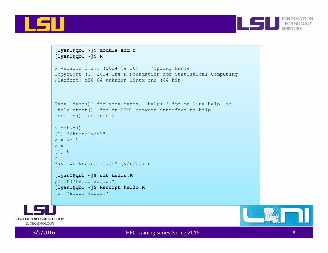
[lyan1@qb1 ~]$ module add r[lyan1@qb1 ~]$ R
R version 3.1.0 (2014-04-10) -- "Spring Dance"Copyright (C) 2014 The R Foundation for Statistical ComputingPlatform: x86_64-unknown-linux-gnu (64-bit)
…
Type 'demo()' for some demos, 'help()' for on-line help, or'help.start()' for an HTML browser interface to help.Type 'q()' to quit R.
> getwd()[1] "/home/lyan1"> x <- 5> x[1] 5>Save workspace image? [y/n/c]: n
[lyan1@qb1 ~]$ cat hello.Rprint("Hello World!")[lyan1@qb1 ~]$ Rscript hello.R[1] "Hello World!"
Installing and Loading R Packages• Installation
– With R Studio• You most likely have root privilege on your own computer• Use the install.packages(“<package name>”) function (double quotation is mandatory), or
• Click on “install packages” in the menu– On a cluster
• You most likely do NOT have root privilege• To install a R packages
– Point the environment variable R_LIBS_USER to desired location, then – Use the install.packages function
• Loading: the library() function load previously installed packages
3/2/2016 HPC training series Spring 2016 9
3/2/2016 HPC training series Spring 2016 10
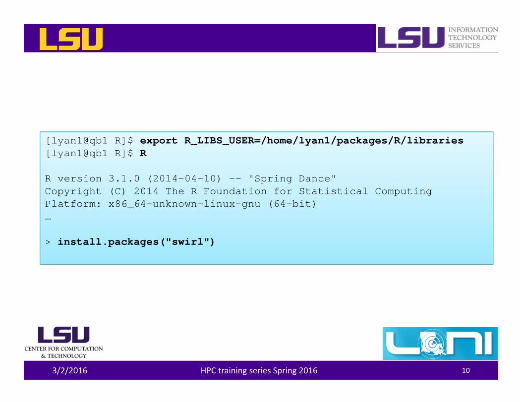
[lyan1@qb1 R]$ export R_LIBS_USER=/home/lyan1/packages/R/libraries[lyan1@qb1 R]$ R
R version 3.1.0 (2014-04-10) -- "Spring Dance"Copyright (C) 2014 The R Foundation for Statistical ComputingPlatform: x86_64-unknown-linux-gnu (64-bit)…
> install.packages("swirl")
Getting Help
• Command line– ?<command name>– ??<part of command name/topic>– help(<function name>)
• Or search in the help page in Rstudio
3/2/2016 HPC training series Spring 2016 11
Data Classes• R has five atomic classes
– Numeric (double)• Numbers in R are treated as numeric unless specified otherwise.
– Integer– Complex– Character– Logical
• TRUE or FALSE• Derivative classes
– Factor– Date and time
• You can convert data from one type to the other using the as.<Type> functions
3/2/2016 HPC training series Spring 2016 12
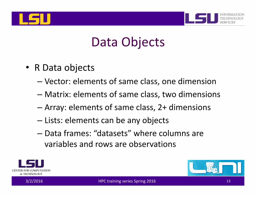
Data Objects
• R Data objects– Vector: elements of same class, one dimension–Matrix: elements of same class, two dimensions– Array: elements of same class, 2+ dimensions– Lists: elements can be any objects– Data frames: “datasets” where columns are variables and rows are observations
3/2/2016 HPC training series Spring 2016 13
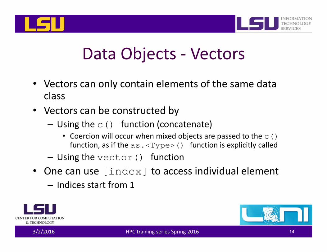
Data Objects ‐ Vectors• Vectors can only contain elements of the same data
class• Vectors can be constructed by
– Using the c() function (concatenate)• Coercion will occur when mixed objects are passed to the c() function, as if the as.<Type>() function is explicitly called
– Using the vector() function• One can use [index] to access individual element
– Indices start from 1
3/2/2016 HPC training series Spring 2016 14
3/2/2016 HPC training series Spring 2016 15
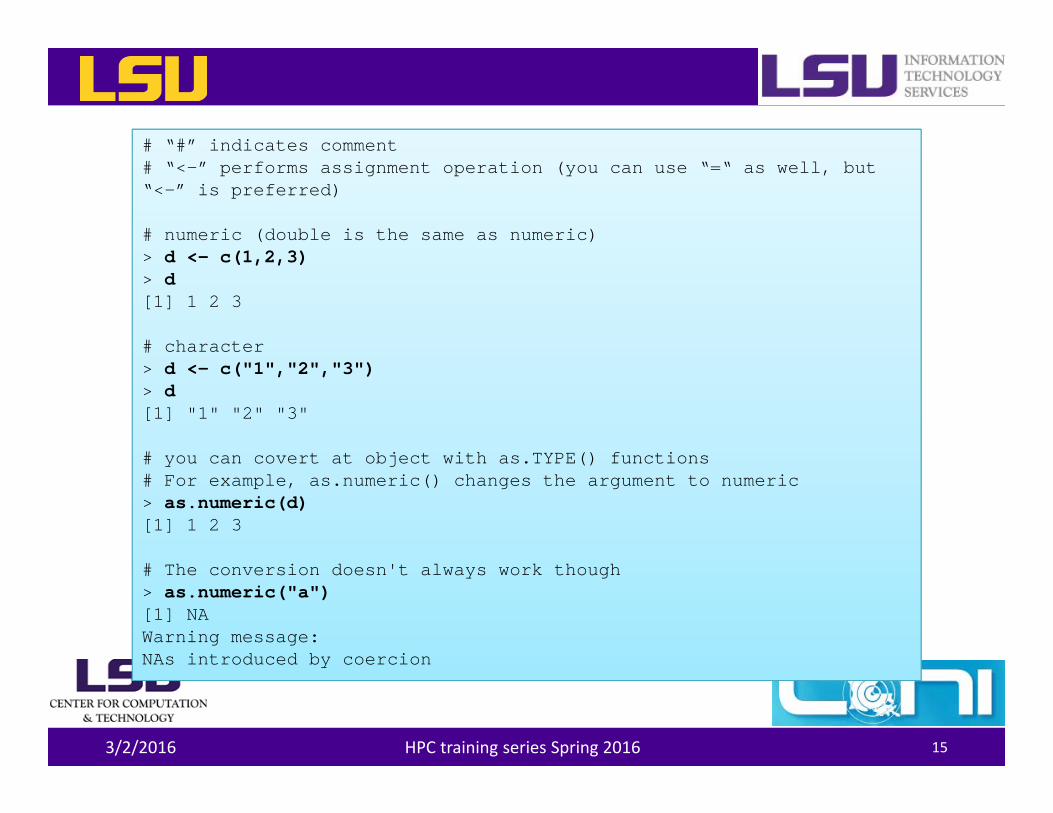
# “#” indicates comment# “<-” performs assignment operation (you can use “=“ as well, but “<-” is preferred)
# numeric (double is the same as numeric)> d <- c(1,2,3)> d[1] 1 2 3
# character> d <- c("1","2","3")> d[1] "1" "2" "3"
# you can covert at object with as.TYPE() functions# For example, as.numeric() changes the argument to numeric> as.numeric(d)[1] 1 2 3
# The conversion doesn't always work though> as.numeric("a")[1] NAWarning message:NAs introduced by coercion
3/2/2016 HPC training series Spring 2016 16
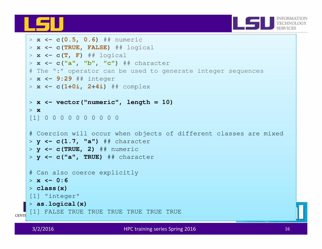
> x <- c(0.5, 0.6) ## numeric> x <- c(TRUE, FALSE) ## logical> x <- c(T, F) ## logical> x <- c("a", "b", "c") ## character# The “:” operator can be used to generate integer sequences> x <- 9:29 ## integer> x <- c(1+0i, 2+4i) ## complex
> x <- vector("numeric", length = 10)> x[1] 0 0 0 0 0 0 0 0 0 0
# Coercion will occur when objects of different classes are mixed> y <- c(1.7, "a") ## character> y <- c(TRUE, 2) ## numeric> y <- c("a", TRUE) ## character
# Can also coerce explicitly> x <- 0:6> class(x)[1] "integer"> as.logical(x)[1] FALSE TRUE TRUE TRUE TRUE TRUE TRUE
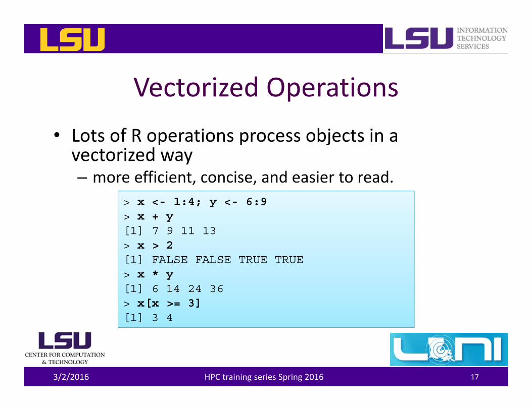
Vectorized Operations• Lots of R operations process objects in a vectorized way– more efficient, concise, and easier to read.
3/2/2016 HPC training series Spring 2016 17
> x <- 1:4; y <- 6:9> x + y[1] 7 9 11 13> x > 2[1] FALSE FALSE TRUE TRUE> x * y[1] 6 14 24 36> x[x >= 3][1] 3 4
Data Objects ‐ Matrices• Matrices are vectors with a dimension attribute• R matrices can be constructed by
– Using the matrix() function– Passing an dim attribute to a vector– Using the cbind() or rbind() functions
• R matrices are constructed column‐wise• One can use [<index>,<index>] to access individual element
3/2/2016 HPC training series Spring 2016 18
3/2/2016 HPC training series Spring 2016 19
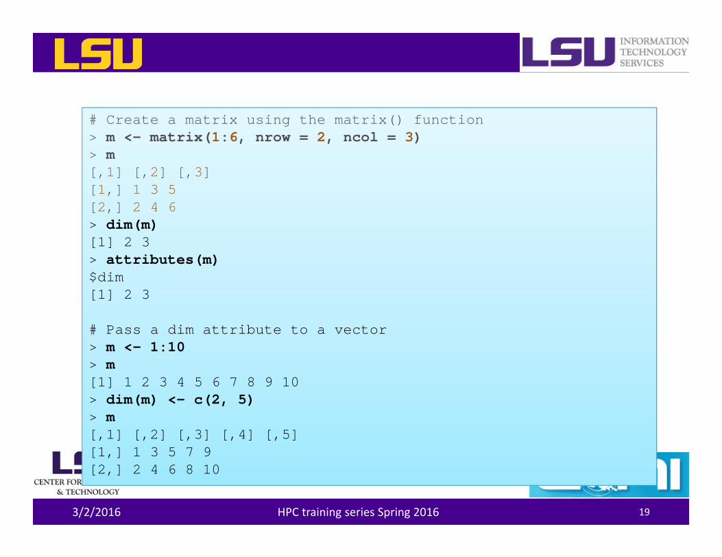
# Create a matrix using the matrix() function> m <- matrix(1:6, nrow = 2, ncol = 3)> m[,1] [,2] [,3][1,] 1 3 5[2,] 2 4 6> dim(m)[1] 2 3> attributes(m)$dim[1] 2 3
# Pass a dim attribute to a vector> m <- 1:10> m[1] 1 2 3 4 5 6 7 8 9 10> dim(m) <- c(2, 5)> m[,1] [,2] [,3] [,4] [,5][1,] 1 3 5 7 9[2,] 2 4 6 8 10
3/2/2016 HPC training series Spring 2016 20
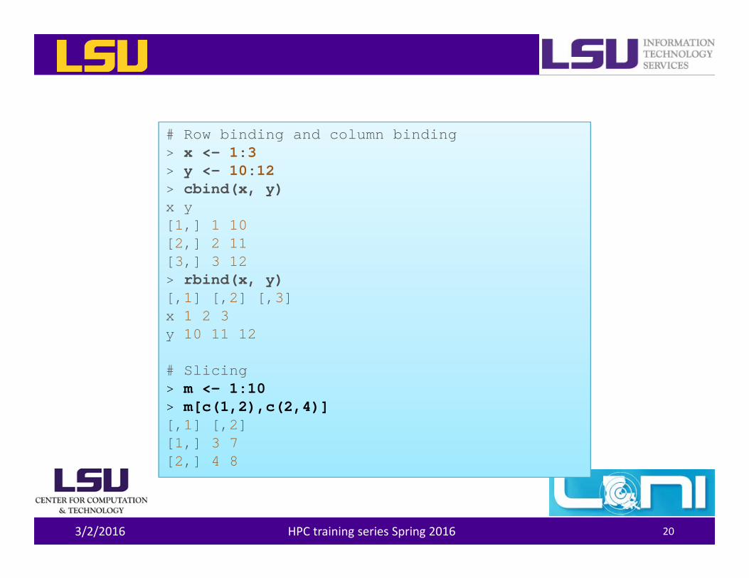
# Row binding and column binding> x <- 1:3> y <- 10:12> cbind(x, y)x y[1,] 1 10[2,] 2 11[3,] 3 12> rbind(x, y)[,1] [,2] [,3]x 1 2 3y 10 11 12
# Slicing > m <- 1:10> m[c(1,2),c(2,4)][,1] [,2][1,] 3 7[2,] 4 8
Data Objects ‐ Lists
• Lists are a ordered collection of objects (that can be different types or classes)
• Lists can be constructed by using the list() function
• Lists can be indexed using [[]]
3/2/2016 HPC training series Spring 2016 21
3/2/2016 HPC training series Spring 2016 22
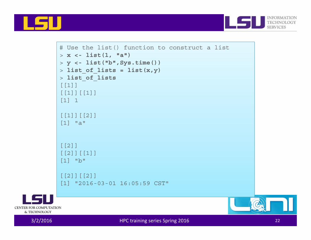
# Use the list() function to construct a list> x <- list(1, "a")> y <- list("b",Sys.time())> list_of_lists = list(x,y)> list_of_lists[[1]][[1]][[1]][1] 1
[[1]][[2]][1] "a"
[[2]][[2]][[1]][1] "b"
[[2]][[2]][1] "2016-03-01 16:05:59 CST"
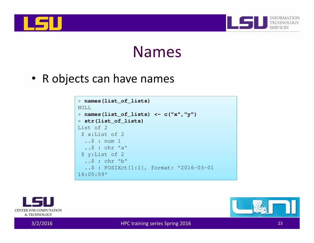
Names• R objects can have names
3/2/2016 HPC training series Spring 2016 23
> names(list_of_lists)NULL> names(list_of_lists) <- c("x","y")> str(list_of_lists)List of 2$ x:List of 2..$ : num 1..$ : chr "a"
$ y:List of 2..$ : chr "b"..$ : POSIXct[1:1], format: "2016-03-01
16:05:59"
3/2/2016 HPC training series Spring 2016 24
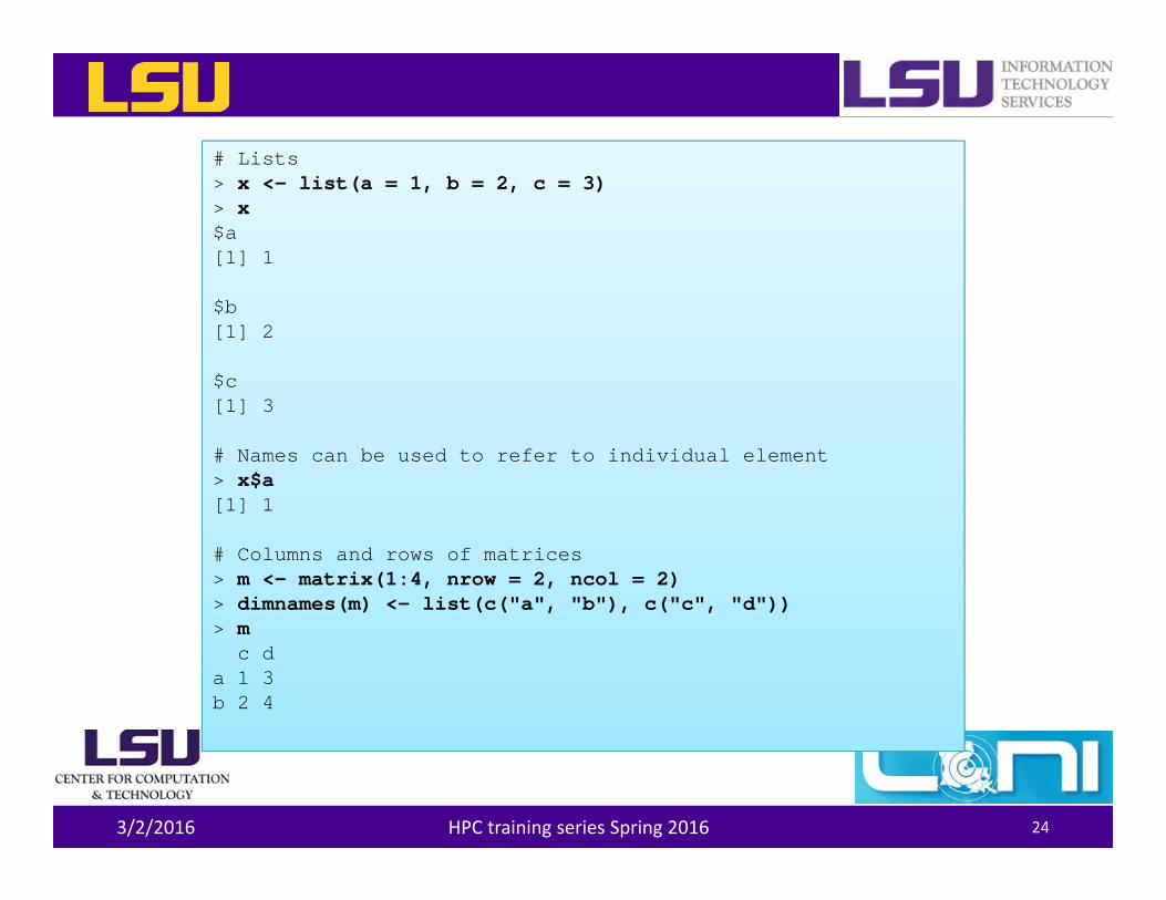
# Lists> x <- list(a = 1, b = 2, c = 3)> x$a[1] 1
$b[1] 2
$c[1] 3
# Names can be used to refer to individual element> x$a[1] 1
# Columns and rows of matrices> m <- matrix(1:4, nrow = 2, ncol = 2)> dimnames(m) <- list(c("a", "b"), c("c", "d"))> m
c da 1 3b 2 4
Data Objects ‐ Data Frames• Data frames are used to store tabular data
– They are a special type of list where every element of the list has to have the same length
– Each element of the list can be thought of as a column – Data frames can store different classes of objects in each
column– Data frames can have special attributes such as row.names– Data frames are usually created by calling read.table() or read.csv()• More on this later
– Can be converted to a matrix by calling data.matrix()
3/2/2016 HPC training series Spring 2016 25
3/2/2016 HPC training series Spring 2016 26
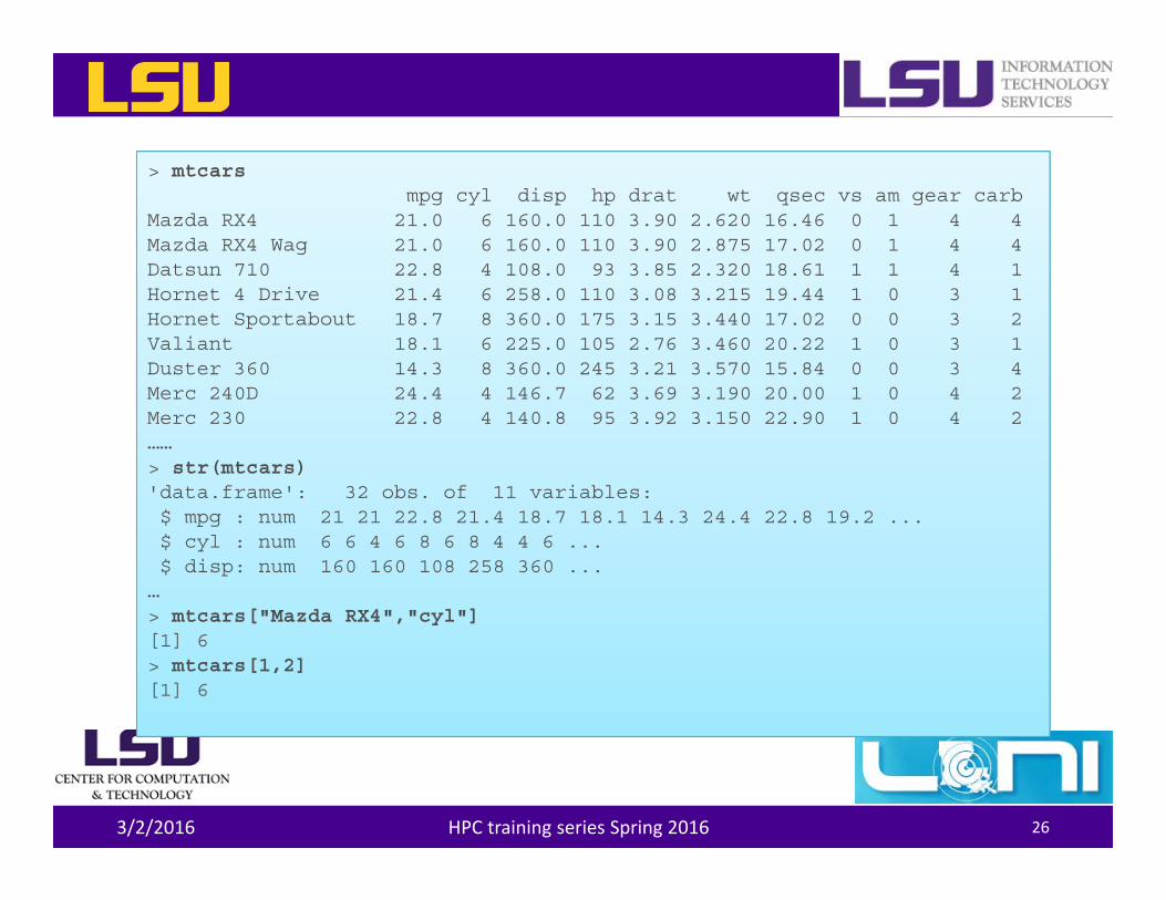
> mtcarsmpg cyl disp hp drat wt qsec vs am gear carb
Mazda RX4 21.0 6 160.0 110 3.90 2.620 16.46 0 1 4 4Mazda RX4 Wag 21.0 6 160.0 110 3.90 2.875 17.02 0 1 4 4Datsun 710 22.8 4 108.0 93 3.85 2.320 18.61 1 1 4 1Hornet 4 Drive 21.4 6 258.0 110 3.08 3.215 19.44 1 0 3 1Hornet Sportabout 18.7 8 360.0 175 3.15 3.440 17.02 0 0 3 2Valiant 18.1 6 225.0 105 2.76 3.460 20.22 1 0 3 1Duster 360 14.3 8 360.0 245 3.21 3.570 15.84 0 0 3 4Merc 240D 24.4 4 146.7 62 3.69 3.190 20.00 1 0 4 2Merc 230 22.8 4 140.8 95 3.92 3.150 22.90 1 0 4 2……> str(mtcars)'data.frame': 32 obs. of 11 variables:$ mpg : num 21 21 22.8 21.4 18.7 18.1 14.3 24.4 22.8 19.2 ...$ cyl : num 6 6 4 6 8 6 8 4 4 6 ...$ disp: num 160 160 108 258 360 ...
…> mtcars["Mazda RX4","cyl"][1] 6> mtcars[1,2][1] 6
Querying Object Attributes• The class() function• The str() function• The attributes() function reveals attributes of an object
(does not work with vectors)– Class– Names– Dimensions– Length– User defined attributes
• They work on all objects (including functions)
3/2/2016 HPC training series Spring 2016 27
3/2/2016 HPC training series Spring 2016 28
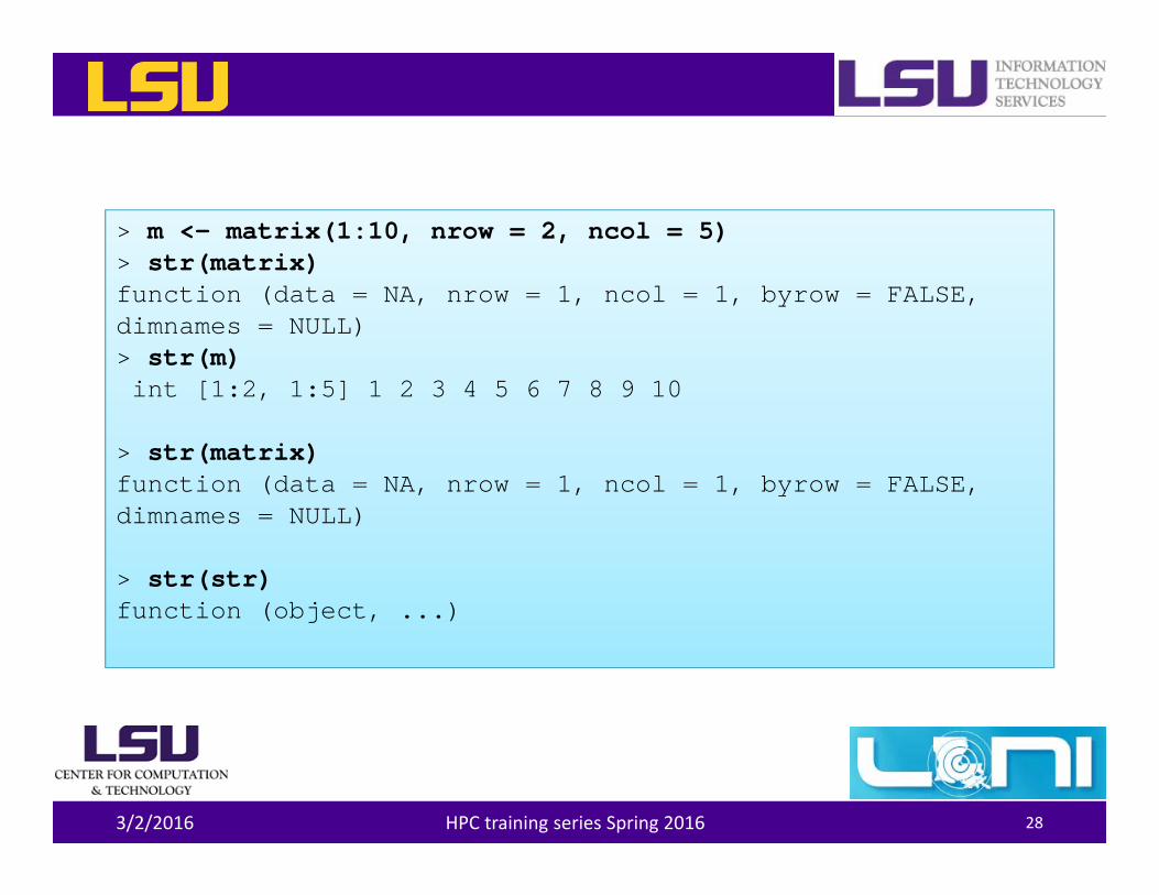
> m <- matrix(1:10, nrow = 2, ncol = 5)> str(matrix)function (data = NA, nrow = 1, ncol = 1, byrow = FALSE, dimnames = NULL)> str(m)int [1:2, 1:5] 1 2 3 4 5 6 7 8 9 10
> str(matrix)function (data = NA, nrow = 1, ncol = 1, byrow = FALSE, dimnames = NULL)
> str(str)function (object, ...)
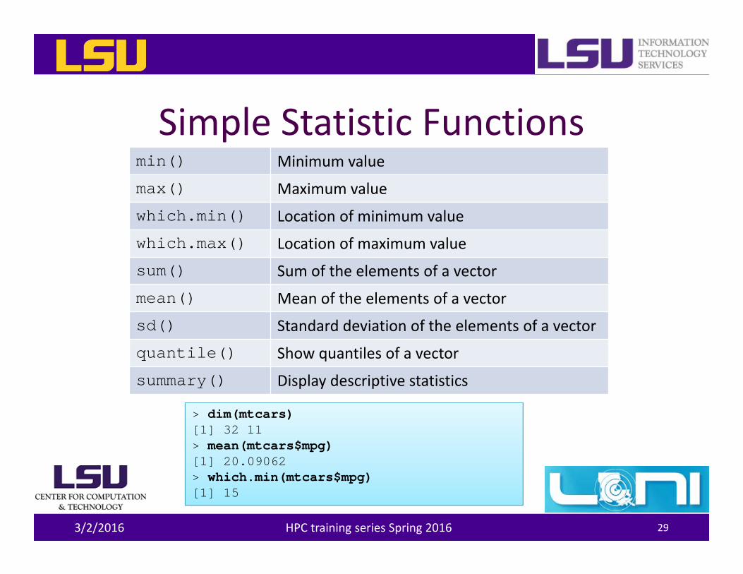
Simple Statistic Functionsmin() Minimum value
max() Maximum value
which.min() Location of minimum value
which.max() Location of maximum value
sum() Sum of the elements of a vector
mean() Mean of the elements of a vector
sd() Standard deviation of the elements of a vector
quantile() Show quantiles of a vector
summary() Display descriptive statistics
3/2/2016 HPC training series Spring 2016 29
> dim(mtcars)[1] 32 11> mean(mtcars$mpg)[1] 20.09062> which.min(mtcars$mpg)[1] 15
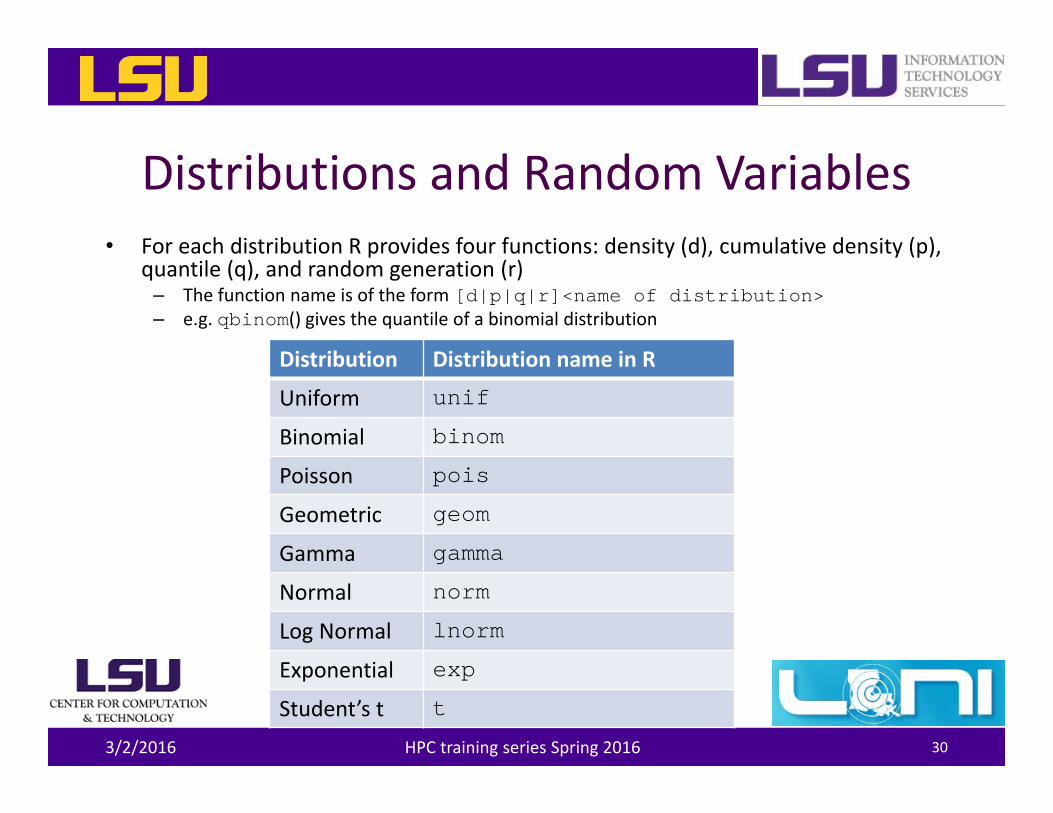
Distributions and Random Variables• For each distribution R provides four functions: density (d), cumulative density (p),
quantile (q), and random generation (r)– The function name is of the form [d|p|q|r]<name of distribution>– e.g. qbinom() gives the quantile of a binomial distribution
3/2/2016 HPC training series Spring 2016 30
Distribution Distribution name in R
Uniform unif
Binomial binom
Poisson pois
Geometric geom
Gamma gamma
Normal norm
Log Normal lnorm
Exponential exp
Student’s t t
3/2/2016 HPC training series Spring 2016 31
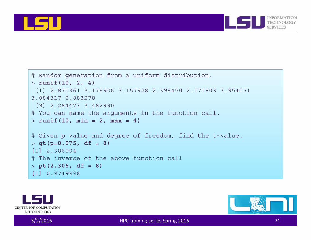
# Random generation from a uniform distribution.> runif(10, 2, 4)[1] 2.871361 3.176906 3.157928 2.398450 2.171803 3.954051 3.084317 2.883278[9] 2.284473 3.482990# You can name the arguments in the function call.> runif(10, min = 2, max = 4)
# Given p value and degree of freedom, find the t-value.> qt(p=0.975, df = 8)[1] 2.306004# The inverse of the above function call> pt(2.306, df = 8)[1] 0.9749998
User Defined Functions
• Similar to other languages, functions in Rare defined by using the function() directives
• The return value is the last expression in the function body to be evaluated.
• Functions can be nested• Functions are R objects
– For example, they can be passed as an argument to other functions
3/2/2016 HPC training series Spring 2016 32
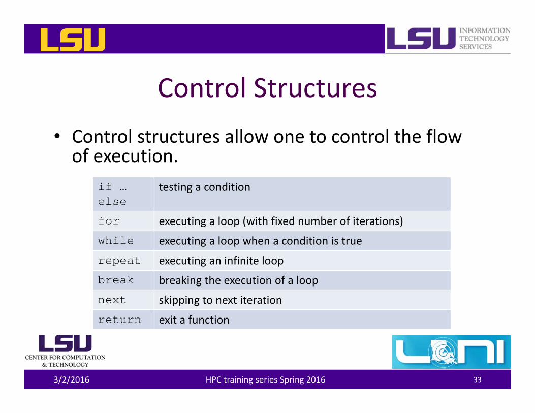
Control Structures• Control structures allow one to control the flow of execution.
3/2/2016 HPC training series Spring 2016 33
if … else
testing a condition
for executing a loop (with fixed number of iterations)
while executing a loop when a condition is true
repeat executing an infinite loop
break breaking the execution of a loop
next skipping to next iteration
return exit a function
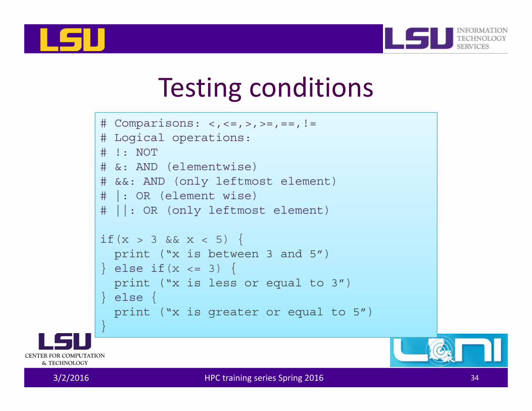
Testing conditions
3/2/2016 HPC training series Spring 2016 34
# Comparisons: <,<=,>,>=,==,!=# Logical operations: # !: NOT# &: AND (elementwise)# &&: AND (only leftmost element)# |: OR (element wise)# ||: OR (only leftmost element)
if(x > 3 && x < 5) {print (“x is between 3 and 5”)
} else if(x <= 3) {print (“x is less or equal to 3”)
} else {print (“x is greater or equal to 5”)
}
Outline
• R basics– Getting started– Data classes and objects
• Data analysis case study: NOAA weather hazard data
3/2/2016 HPC training series Spring 2016 35
Steps for Data Analysis
• Get the data • Read and inspect the data• Preprocess the data (remove missing and dubious values, discard columns not needed etc.)
• Analyze the data• Generate a report
3/2/2016 HPC training series Spring 2016 36

Case Study: NOAA Weather Hazard Data
• Hazardous weather event data from US National Oceanic and Atmospheric Administration– Records time, location, damage etc. for all hazardous weather events in theUS between year 1950 and 2011
– BZ2 compressed CSV data• Objectives
– Rank the type of events according to their threat to public health (fatalities plus injuries per occurrence)• Report the top 10 types of events• Generate a plot for the result
3/2/2016 HPC training series Spring 2016 37

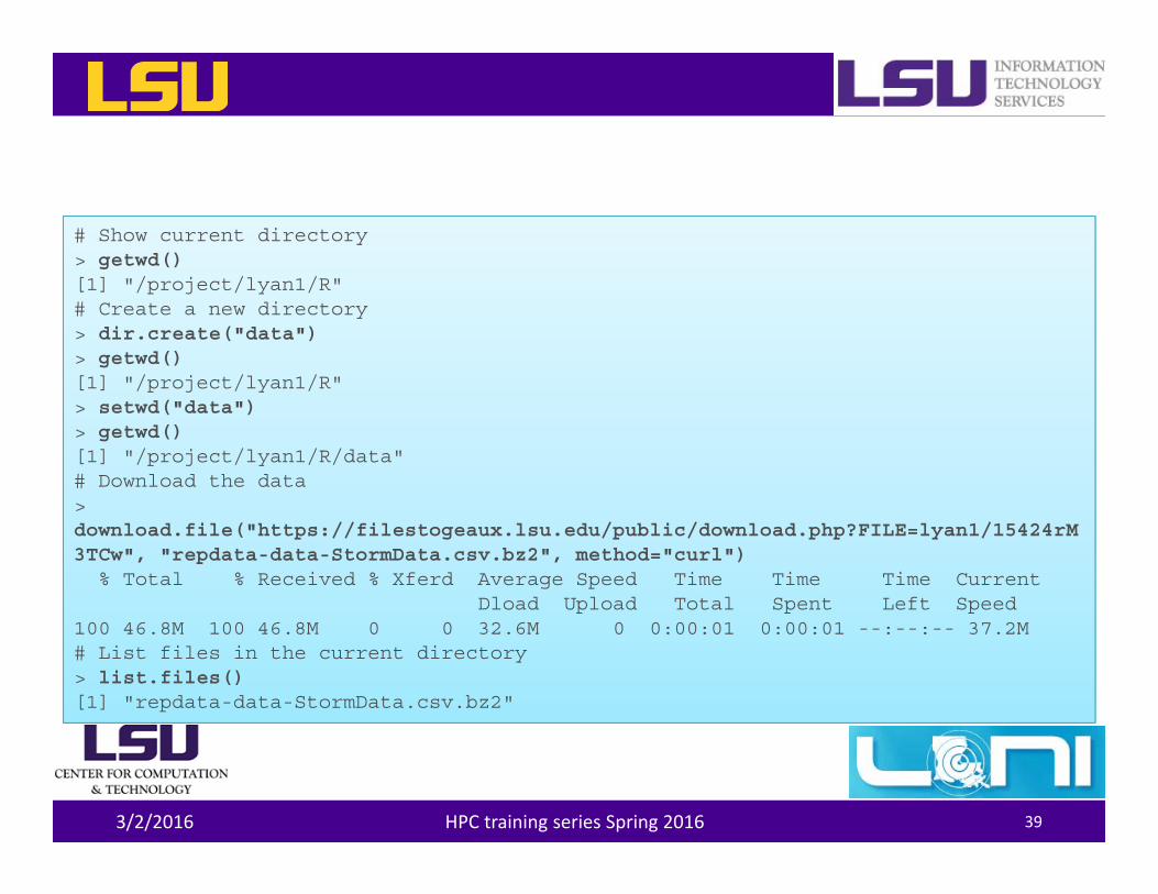
Getting Data
• Display and set current working directory– getwd() and setwd()
• Downloading files from internet– download.file()
• File manipulation– file.exists(), list.files() and dir.create()
3/2/2016 HPC training series Spring 2016 38
3/2/2016 HPC training series Spring 2016 39
# Show current directory> getwd()[1] "/project/lyan1/R"# Create a new directory> dir.create("data")> getwd()[1] "/project/lyan1/R"> setwd("data")> getwd()[1] "/project/lyan1/R/data"# Download the data > download.file("https://filestogeaux.lsu.edu/public/download.php?FILE=lyan1/15424rM3TCw", "repdata-data-StormData.csv.bz2", method="curl")
% Total % Received % Xferd Average Speed Time Time Time CurrentDload Upload Total Spent Left Speed
100 46.8M 100 46.8M 0 0 32.6M 0 0:00:01 0:00:01 --:--:-- 37.2M# List files in the current directory> list.files()[1] "repdata-data-StormData.csv.bz2"
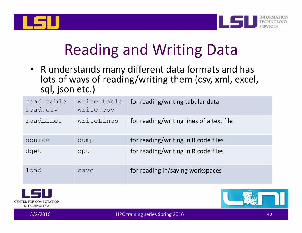
Reading and Writing Data• R understands many different data formats and has
lots of ways of reading/writing them (csv, xml, excel, sql, json etc.)
3/2/2016 HPC training series Spring 2016 40
read.tableread.csv
write.tablewrite.csv
for reading/writing tabular data
readLines writeLines for reading/writing lines of a text file
source dump for reading/writing in R code files
dget dput for reading/writing in R code files
load save for reading in/saving workspaces
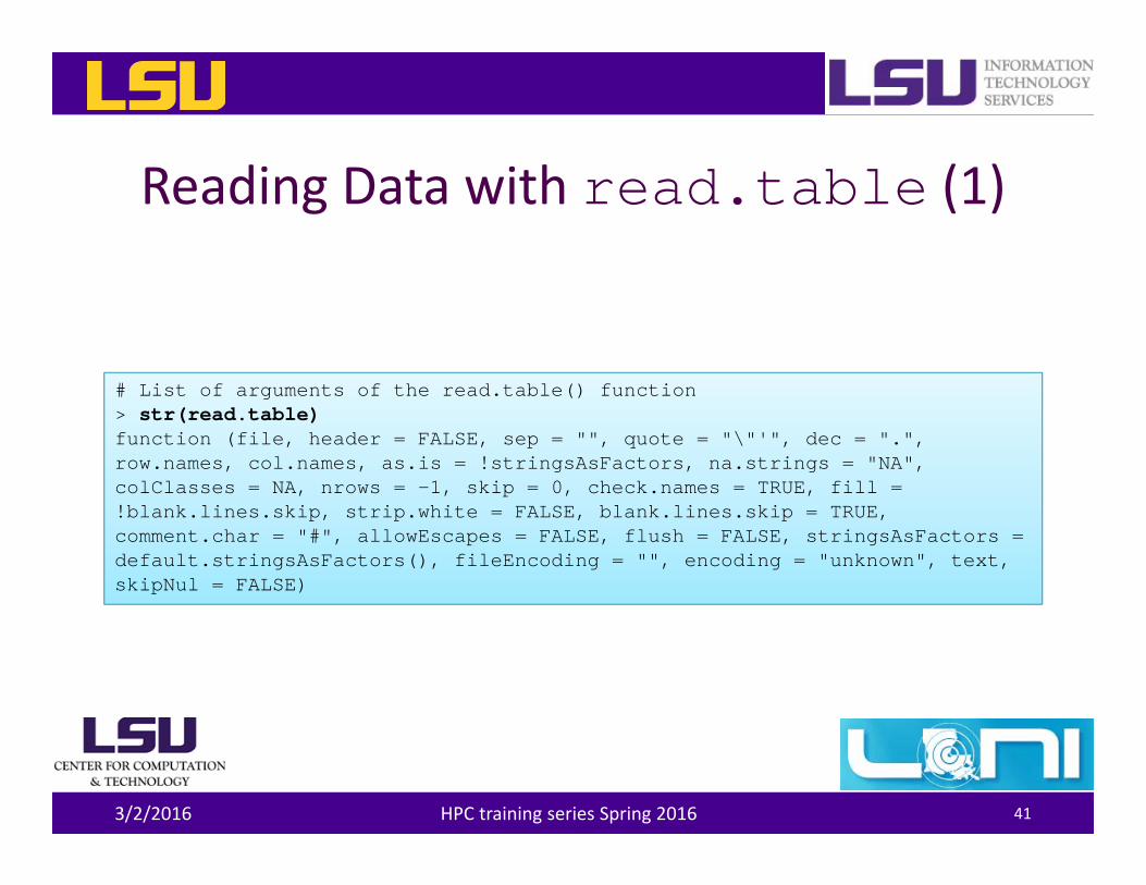
Reading Data with read.table (1)
3/2/2016 HPC training series Spring 2016 41
# List of arguments of the read.table() function> str(read.table)function (file, header = FALSE, sep = "", quote = "\"'", dec = ".", row.names, col.names, as.is = !stringsAsFactors, na.strings = "NA", colClasses = NA, nrows = -1, skip = 0, check.names = TRUE, fill = !blank.lines.skip, strip.white = FALSE, blank.lines.skip = TRUE, comment.char = "#", allowEscapes = FALSE, flush = FALSE, stringsAsFactors = default.stringsAsFactors(), fileEncoding = "", encoding = "unknown", text, skipNul = FALSE)
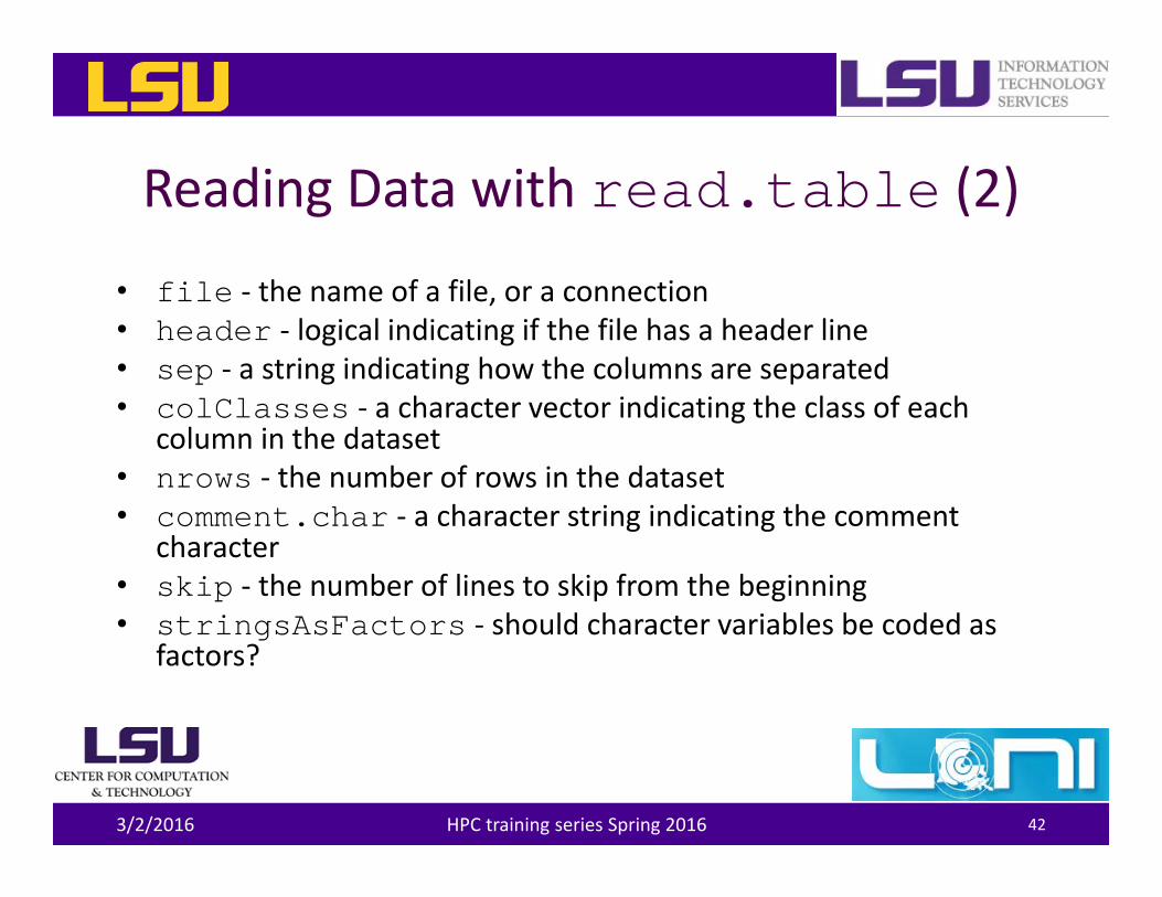
Reading Data with read.table (2)
• file ‐ the name of a file, or a connection• header ‐ logical indicating if the file has a header line• sep ‐ a string indicating how the columns are separated• colClasses ‐ a character vector indicating the class of each
column in the dataset• nrows ‐ the number of rows in the dataset• comment.char ‐ a character string indicating the comment
character• skip ‐ the number of lines to skip from the beginning• stringsAsFactors ‐ should character variables be coded as
factors?
3/2/2016 HPC training series Spring 2016 42
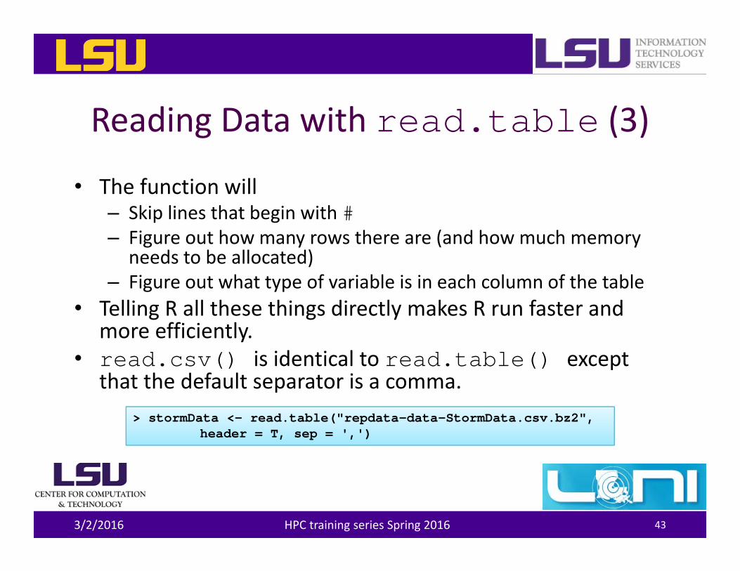
Reading Data with read.table (3)
• The function will– Skip lines that begin with #– Figure out how many rows there are (and how much memory
needs to be allocated)– Figure out what type of variable is in each column of the table
• Telling R all these things directly makes R run faster and more efficiently.
• read.csv() is identical to read.table() except that the default separator is a comma.
3/2/2016 HPC training series Spring 2016 43
> stormData <- read.table("repdata-data-StormData.csv.bz2", header = T, sep = ',')
Inspecting Data (1)
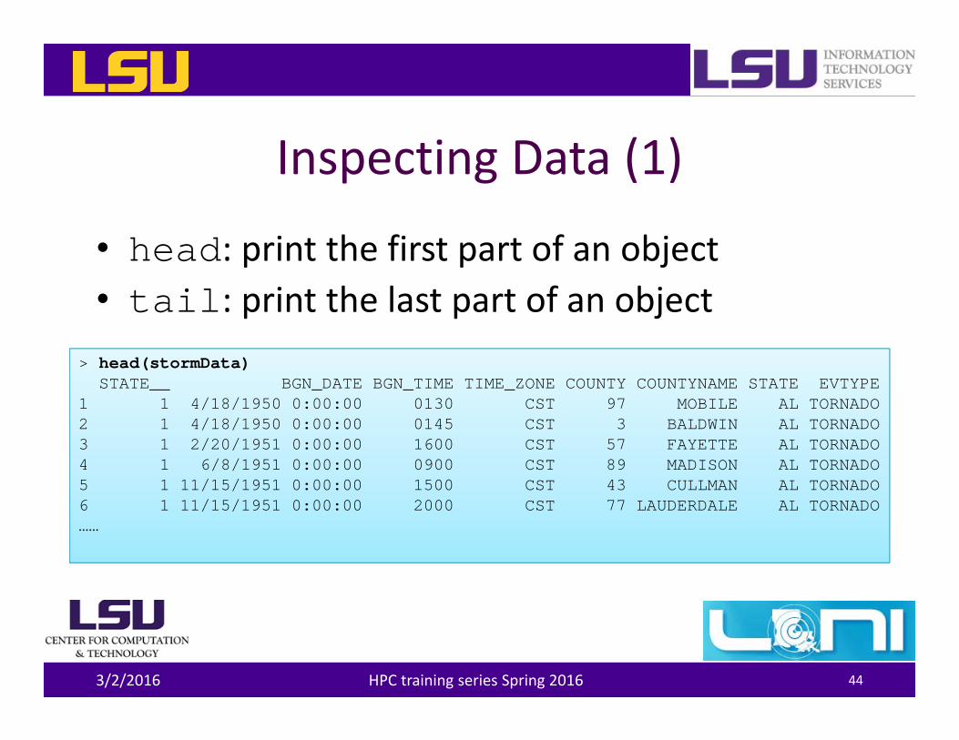
• head: print the first part of an object• tail: print the last part of an object
3/2/2016 HPC training series Spring 2016 44
> head(stormData)STATE__ BGN_DATE BGN_TIME TIME_ZONE COUNTY COUNTYNAME STATE EVTYPE
1 1 4/18/1950 0:00:00 0130 CST 97 MOBILE AL TORNADO2 1 4/18/1950 0:00:00 0145 CST 3 BALDWIN AL TORNADO3 1 2/20/1951 0:00:00 1600 CST 57 FAYETTE AL TORNADO4 1 6/8/1951 0:00:00 0900 CST 89 MADISON AL TORNADO5 1 11/15/1951 0:00:00 1500 CST 43 CULLMAN AL TORNADO6 1 11/15/1951 0:00:00 2000 CST 77 LAUDERDALE AL TORNADO……
Inspecting Data (2)
3/2/2016 HPC training series Spring 2016 45
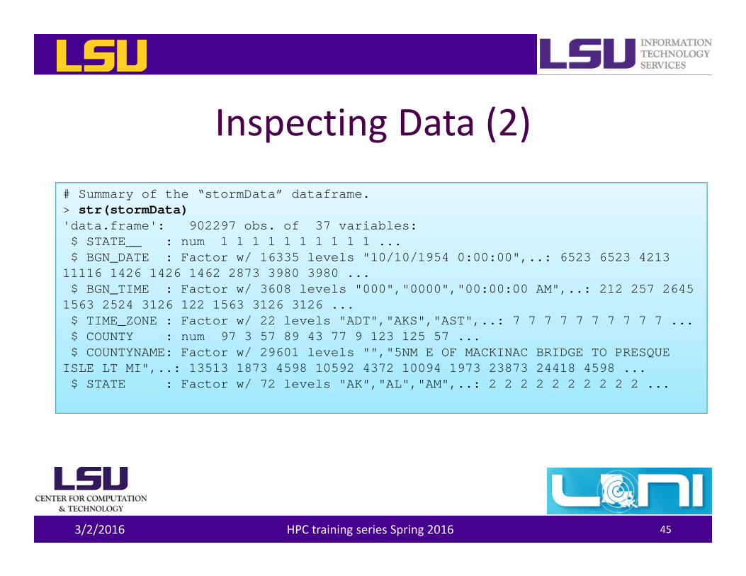
# Summary of the “stormData” dataframe.> str(stormData)'data.frame': 902297 obs. of 37 variables:$ STATE__ : num 1 1 1 1 1 1 1 1 1 1 ...$ BGN_DATE : Factor w/ 16335 levels "10/10/1954 0:00:00",..: 6523 6523 4213
11116 1426 1426 1462 2873 3980 3980 ...$ BGN_TIME : Factor w/ 3608 levels "000","0000","00:00:00 AM",..: 212 257 2645
1563 2524 3126 122 1563 3126 3126 ...$ TIME_ZONE : Factor w/ 22 levels "ADT","AKS","AST",..: 7 7 7 7 7 7 7 7 7 7 ...$ COUNTY : num 97 3 57 89 43 77 9 123 125 57 ...$ COUNTYNAME: Factor w/ 29601 levels "","5NM E OF MACKINAC BRIDGE TO PRESQUE
ISLE LT MI",..: 13513 1873 4598 10592 4372 10094 1973 23873 24418 4598 ...$ STATE : Factor w/ 72 levels "AK","AL","AM",..: 2 2 2 2 2 2 2 2 2 2 ...
Inspecting Data (3)
3/2/2016 HPC training series Spring 2016 46
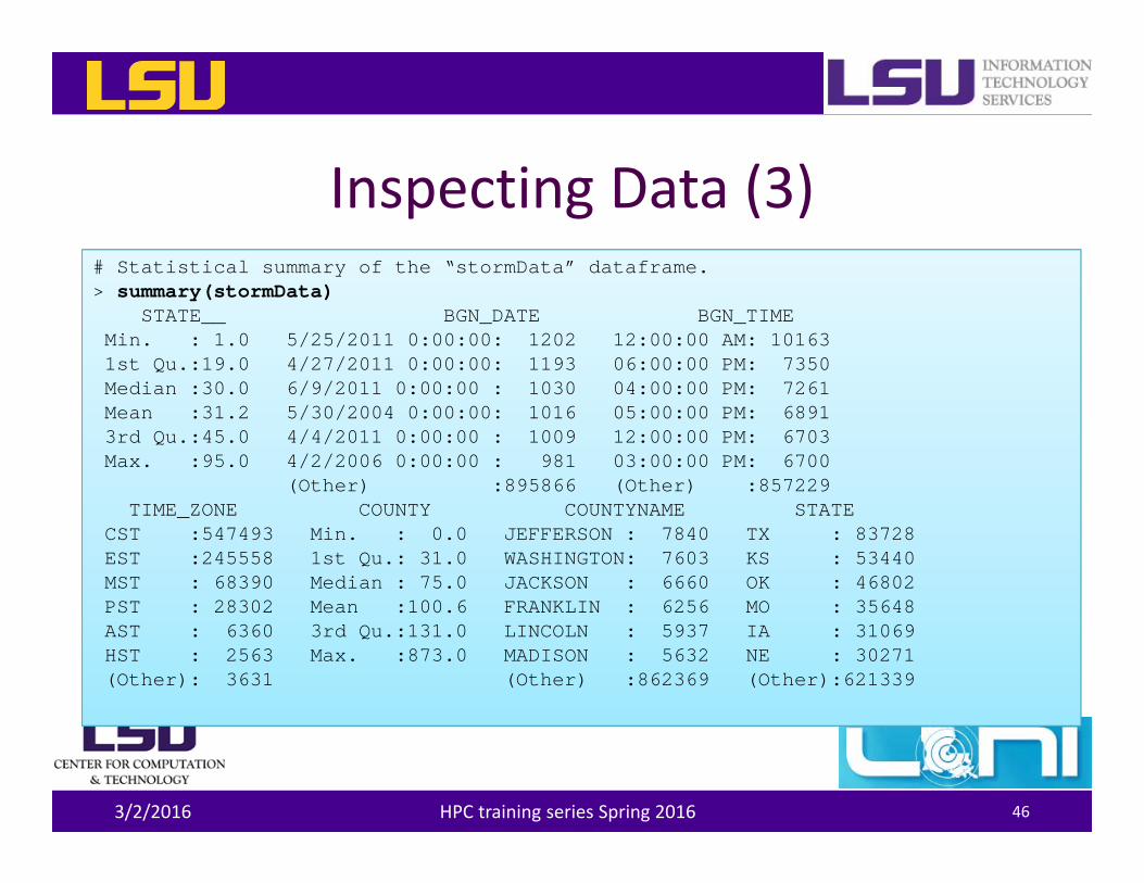
# Statistical summary of the “stormData” dataframe.> summary(stormData)
STATE__ BGN_DATE BGN_TIMEMin. : 1.0 5/25/2011 0:00:00: 1202 12:00:00 AM: 101631st Qu.:19.0 4/27/2011 0:00:00: 1193 06:00:00 PM: 7350Median :30.0 6/9/2011 0:00:00 : 1030 04:00:00 PM: 7261Mean :31.2 5/30/2004 0:00:00: 1016 05:00:00 PM: 68913rd Qu.:45.0 4/4/2011 0:00:00 : 1009 12:00:00 PM: 6703Max. :95.0 4/2/2006 0:00:00 : 981 03:00:00 PM: 6700
(Other) :895866 (Other) :857229TIME_ZONE COUNTY COUNTYNAME STATE
CST :547493 Min. : 0.0 JEFFERSON : 7840 TX : 83728EST :245558 1st Qu.: 31.0 WASHINGTON: 7603 KS : 53440MST : 68390 Median : 75.0 JACKSON : 6660 OK : 46802PST : 28302 Mean :100.6 FRANKLIN : 6256 MO : 35648AST : 6360 3rd Qu.:131.0 LINCOLN : 5937 IA : 31069HST : 2563 Max. :873.0 MADISON : 5632 NE : 30271(Other): 3631 (Other) :862369 (Other):621339
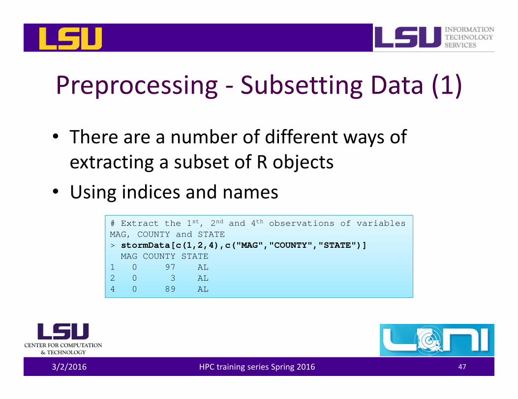
Preprocessing ‐ Subsetting Data (1)
• There are a number of different ways of extracting a subset of R objects
• Using indices and names
3/2/2016 HPC training series Spring 2016 47
# Extract the 1st, 2nd and 4th observations of variables MAG, COUNTY and STATE> stormData[c(1,2,4),c("MAG","COUNTY","STATE")]
MAG COUNTY STATE1 0 97 AL2 0 3 AL4 0 89 AL
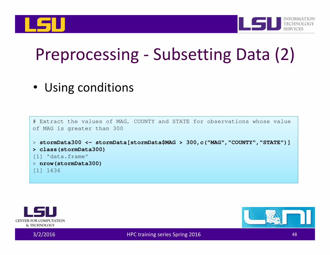
Preprocessing ‐ Subsetting Data (2)
• Using conditions
3/2/2016 HPC training series Spring 2016 48
# Extract the values of MAG, COUNTY and STATE for observations whose value of MAG is greater than 300
> stormData300 <- stormData[stormData$MAG > 300,c("MAG","COUNTY","STATE")]> class(stormData300)[1] "data.frame"> nrow(stormData300)[1] 1636
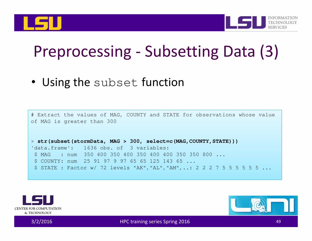
Preprocessing ‐ Subsetting Data (3)
• Using the subset function
3/2/2016 HPC training series Spring 2016 49
# Extract the values of MAG, COUNTY and STATE for observations whose value of MAG is greater than 300
> str(subset(stormData, MAG > 300, select=c(MAG,COUNTY,STATE)))'data.frame': 1636 obs. of 3 variables:$ MAG : num 350 400 350 400 350 400 400 350 350 800 ...$ COUNTY: num 25 91 97 9 97 65 65 125 143 65 ...$ STATE : Factor w/ 72 levels "AK","AL","AM",..: 2 2 2 7 5 5 5 5 5 5 ...
Dealing with Missing Values• Missing values are denoted in R by NA or NaN for undefined
mathematical operations.– is.na() is used to test objects if they are NA– is.nan() is used to test for NaN– NA values have a class also, so there are integer NA, character NA, etc.– A NaN value is also NA but the converse is not true
• The complete.cases() function can be used to identify complete observations
• Many R functions have a logical “na.rm” option– na.rm=TRUEmeans the NA values should be discarded
• Not all missing values are marked with “NA” in raw data
3/2/2016 HPC training series Spring 2016 50
3/2/2016 HPC training series Spring 2016 51
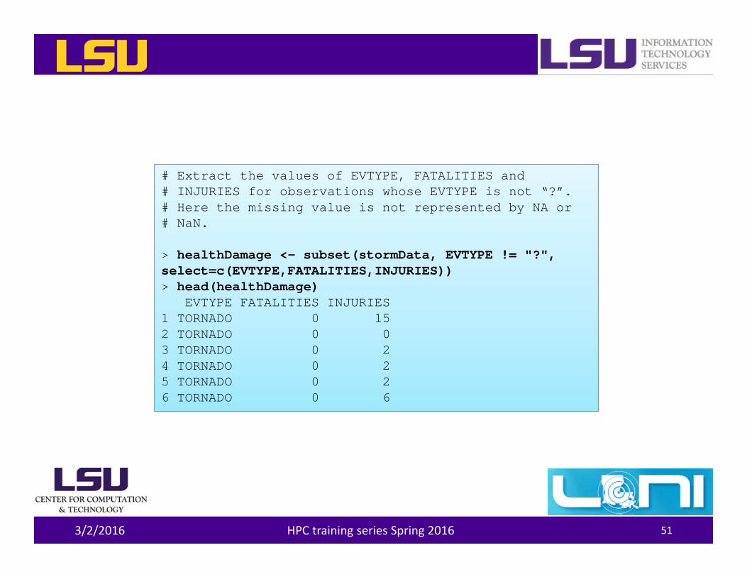
# Extract the values of EVTYPE, FATALITIES and # INJURIES for observations whose EVTYPE is not “?”.# Here the missing value is not represented by NA or # NaN.
> healthDamage <- subset(stormData, EVTYPE != "?", select=c(EVTYPE,FATALITIES,INJURIES))> head(healthDamage)
EVTYPE FATALITIES INJURIES1 TORNADO 0 152 TORNADO 0 03 TORNADO 0 24 TORNADO 0 25 TORNADO 0 26 TORNADO 0 6
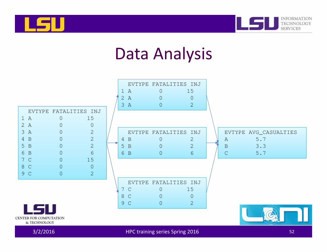
Data Analysis
3/2/2016 HPC training series Spring 2016 52
EVTYPE FATALITIES INJ1 A 0 152 A 0 03 A 0 24 B 0 25 B 0 26 B 0 67 C 0 158 C 0 09 C 0 2
EVTYPE FATALITIES INJ1 A 0 152 A 0 03 A 0 2
EVTYPE FATALITIES INJ4 B 0 25 B 0 26 B 0 6
EVTYPE FATALITIES INJ7 C 0 158 C 0 09 C 0 2
EVTYPE AVG_CASUALTIESA 5.7B 3.3C 5.7
Split‐Apply‐Combine
• In data analysis you often need to split up a big data structure into homogeneous pieces, apply a function to each piece and then combine all the results back together
• This split‐apply‐combine procedure is what the plyr package is for.
3/2/2016 HPC training series Spring 2016 53
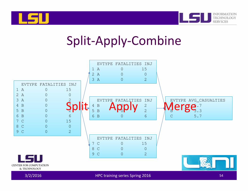
Split‐Apply‐Combine
3/2/2016 HPC training series Spring 2016 54
EVTYPE FATALITIES INJ1 A 0 152 A 0 03 A 0 24 B 0 25 B 0 26 B 0 67 C 0 158 C 0 09 C 0 2
EVTYPE FATALITIES INJ1 A 0 152 A 0 03 A 0 2
EVTYPE FATALITIES INJ4 B 0 25 B 0 26 B 0 6
EVTYPE FATALITIES INJ7 C 0 158 C 0 09 C 0 2
EVTYPE AVG_CASUALTIESA 5.7B 3.3C 5.7
Split Apply Merge
3/2/2016 HPC training series Spring 2016 55
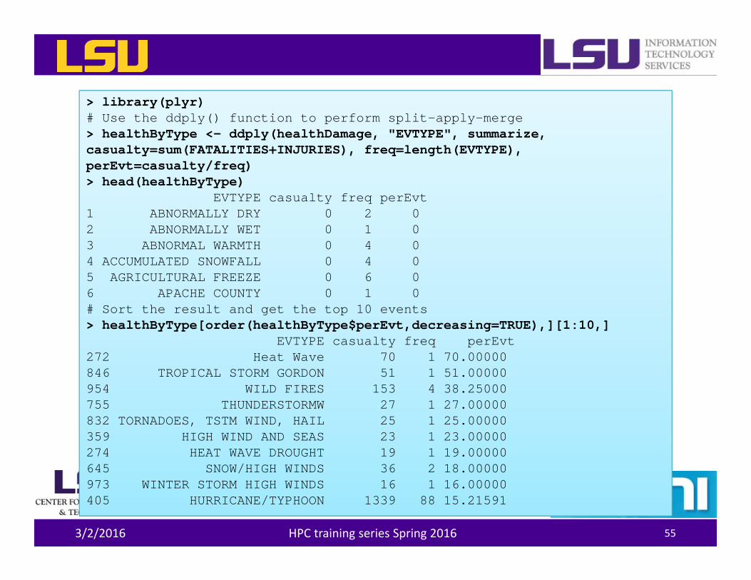
> library(plyr)# Use the ddply() function to perform split-apply-merge> healthByType <- ddply(healthDamage, "EVTYPE", summarize, casualty=sum(FATALITIES+INJURIES), freq=length(EVTYPE), perEvt=casualty/freq)> head(healthByType)
EVTYPE casualty freq perEvt1 ABNORMALLY DRY 0 2 02 ABNORMALLY WET 0 1 03 ABNORMAL WARMTH 0 4 04 ACCUMULATED SNOWFALL 0 4 05 AGRICULTURAL FREEZE 0 6 06 APACHE COUNTY 0 1 0# Sort the result and get the top 10 events> healthByType[order(healthByType$perEvt,decreasing=TRUE),][1:10,]
EVTYPE casualty freq perEvt272 Heat Wave 70 1 70.00000846 TROPICAL STORM GORDON 51 1 51.00000954 WILD FIRES 153 4 38.25000755 THUNDERSTORMW 27 1 27.00000832 TORNADOES, TSTM WIND, HAIL 25 1 25.00000359 HIGH WIND AND SEAS 23 1 23.00000274 HEAT WAVE DROUGHT 19 1 19.00000645 SNOW/HIGH WINDS 36 2 18.00000973 WINTER STORM HIGH WINDS 16 1 16.00000405 HURRICANE/TYPHOON 1339 88 15.21591
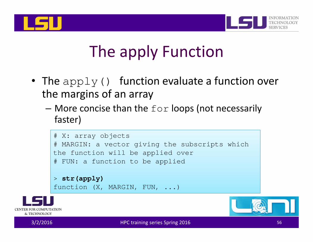
The apply Function
• The apply() function evaluate a function over the margins of an array – More concise than the for loops (not necessarily faster)
3/2/2016 HPC training series Spring 2016 56
# X: array objects# MARGIN: a vector giving the subscripts which the function will be applied over# FUN: a function to be applied
> str(apply)function (X, MARGIN, FUN, ...)
3/2/2016 HPC training series Spring 2016 57
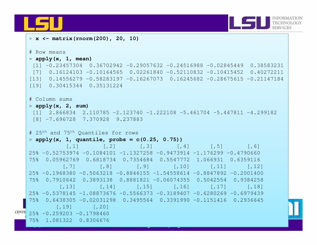
> x <- matrix(rnorm(200), 20, 10)
# Row means> apply(x, 1, mean)[1] -0.23457304 0.36702942 -0.29057632 -0.24516988 -0.02845449 0.38583231[7] 0.16124103 -0.10164565 0.02261840 -0.52110832 -0.10415452 0.40272211
[13] 0.14556279 -0.58283197 -0.16267073 0.16245682 -0.28675615 -0.21147184[19] 0.30415344 0.35131224
# Column sums> apply(x, 2, sum)[1] 2.866834 2.110785 -2.123740 -1.222108 -5.461704 -5.447811 -4.299182[8] -7.696728 7.370928 9.237883
# 25th and 75th Quantiles for rows> apply(x, 1, quantile, probs = c(0.25, 0.75))
[,1] [,2] [,3] [,4] [,5] [,6]25% -0.52753974 -0.1084101 -1.1327258 -0.9473914 -1.176299 -0.479066075% 0.05962769 0.6818734 0.7354684 0.5547772 1.066931 0.6359116
[,7] [,8] [,9] [,10] [,11] [,12]25% -0.1968380 -0.5063218 -0.8846155 -1.54558614 -0.8847892 -0.200140075% 0.7910642 0.3893138 0.8881821 -0.06074355 0.5042554 0.9384258
[,13] [,14] [,15] [,16] [,17] [,18]25% -0.5378145 -1.08873676 -0.5566373 -0.3189407 -0.6280269 -0.697943975% 0.6438305 -0.02031298 0.3495564 0.3391990 -0.1151416 0.2936645
[,19] [,20]25% -0.259203 -0.179846075% 1.081322 0.8306676
3/2/2016 HPC training series Spring 2016 58
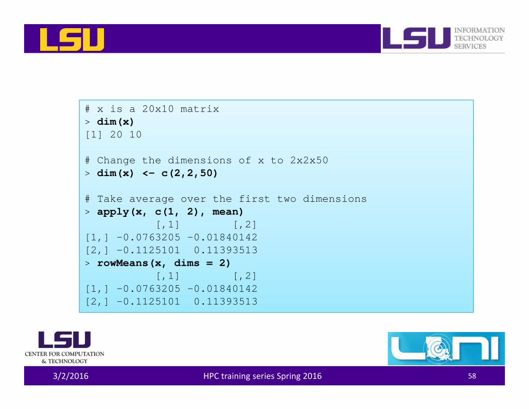
# x is a 20x10 matrix> dim(x)[1] 20 10
# Change the dimensions of x to 2x2x50> dim(x) <- c(2,2,50)
# Take average over the first two dimensions> apply(x, c(1, 2), mean)
[,1] [,2][1,] -0.0763205 -0.01840142[2,] -0.1125101 0.11393513> rowMeans(x, dims = 2)
[,1] [,2][1,] -0.0763205 -0.01840142[2,] -0.1125101 0.11393513
Other Apply Functions
• lapply ‐ Loop over a list and evaluate a function on each element
• sapply ‐ Same as lapply but try to simplify the result
• tapply ‐ Apply a function over subsets of a vector
• mapply ‐ Multivariate version of lapply
3/2/2016 HPC training series Spring 2016 59
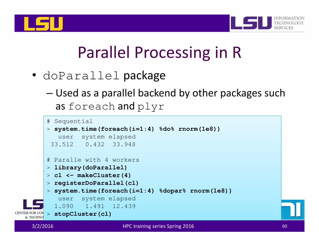
Parallel Processing in R• doParallel package
– Used as a parallel backend by other packages such as foreach and plyr
3/2/2016 HPC training series Spring 2016 60
# Sequential> system.time(foreach(i=1:4) %do% rnorm(1e8))
user system elapsed33.512 0.432 33.948
# Paralle with 4 workers> library(doParallel)> cl <- makeCluster(4)> registerDoParallel(cl)> system.time(foreach(i=1:4) %dopar% rnorm(1e8))
user system elapsed1.090 1.491 12.439
> stopCluster(cl)
3/2/2016 HPC training series Spring 2016 61
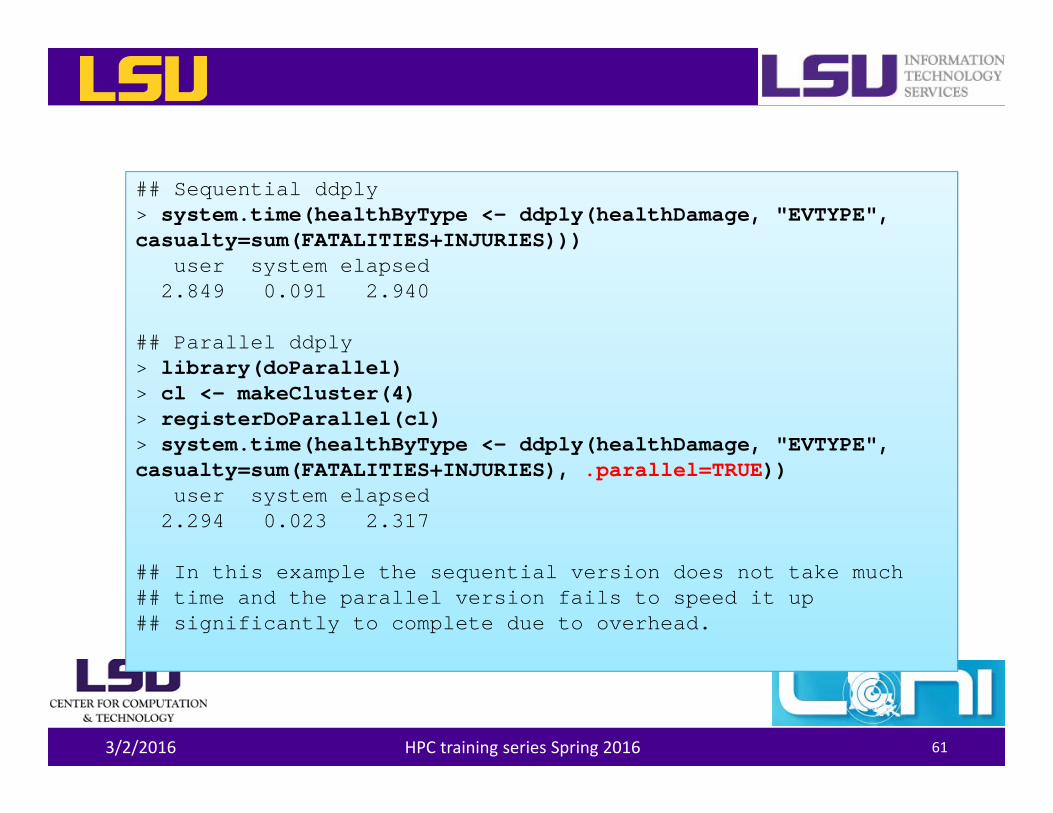
## Sequential ddply> system.time(healthByType <- ddply(healthDamage, "EVTYPE", casualty=sum(FATALITIES+INJURIES)))
user system elapsed2.849 0.091 2.940
## Parallel ddply> library(doParallel)> cl <- makeCluster(4)> registerDoParallel(cl)> system.time(healthByType <- ddply(healthDamage, "EVTYPE", casualty=sum(FATALITIES+INJURIES), .parallel=TRUE))
user system elapsed2.294 0.023 2.317
## In this example the sequential version does not take much## time and the parallel version fails to speed it up ## significantly to complete due to overhead.
Graphics in R• There are three plotting systems in R
– base• Convenient, but hard to adjust after the plot is created
– lattice• Good for creating conditioning plot
– ggplot2• Powerful and flexible, many tunable feature, may require some time to master
• Each has its pros and cons, so it is up to the users which one to choose
3/2/2016 HPC training series Spring 2016 62
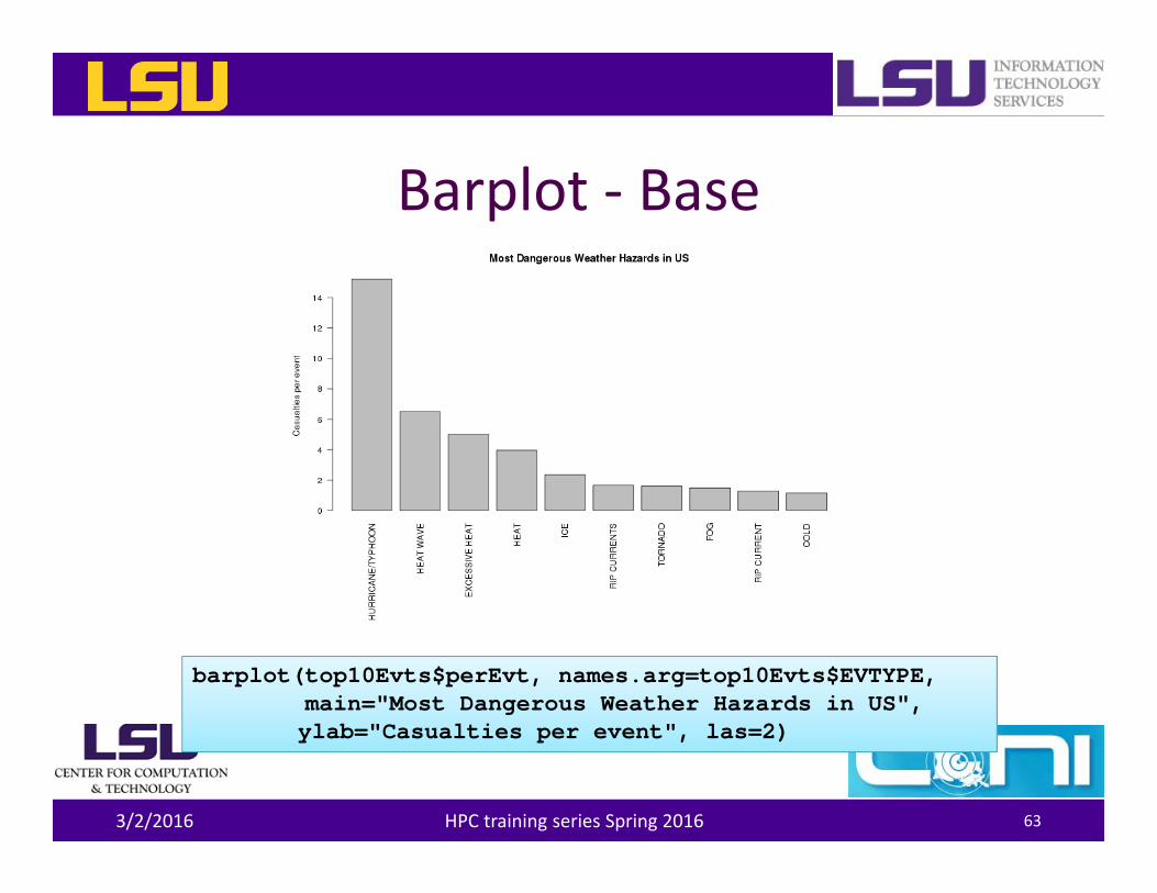
Barplot ‐ Base
3/2/2016 HPC training series Spring 2016 63
barplot(top10Evts$perEvt, names.arg=top10Evts$EVTYPE,main="Most Dangerous Weather Hazards in US",ylab="Casualties per event", las=2)
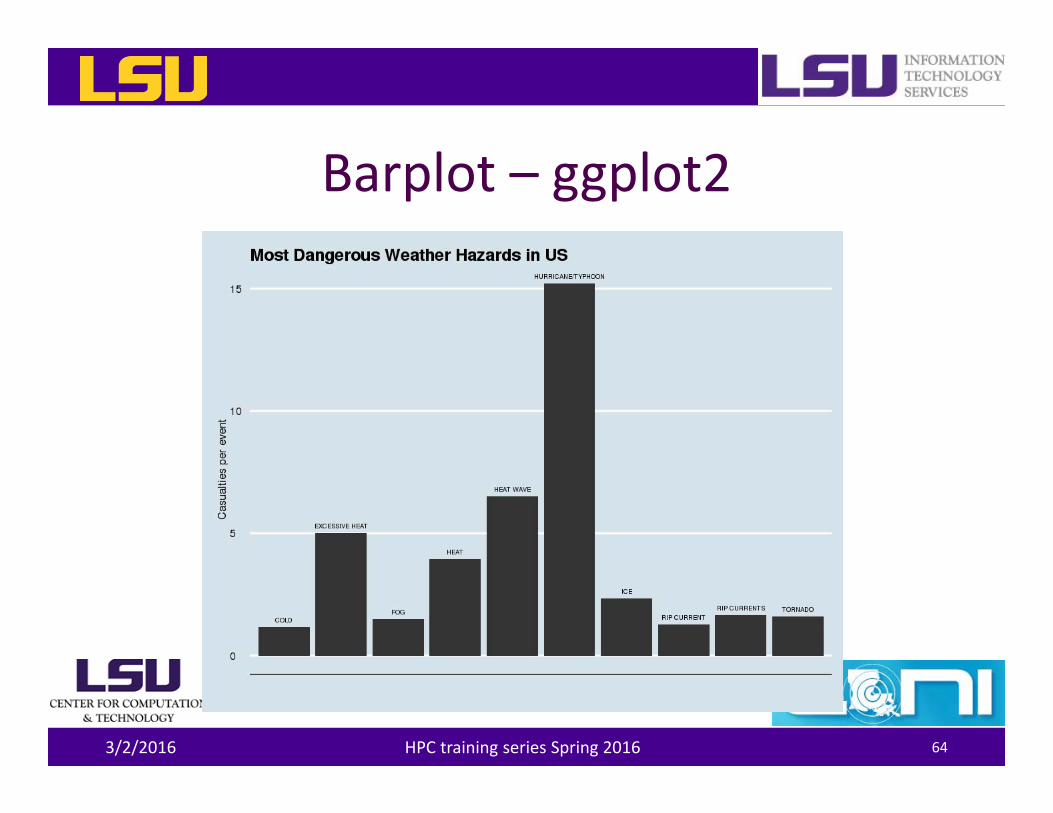
Barplot – ggplot2
3/2/2016 HPC training series Spring 2016 64
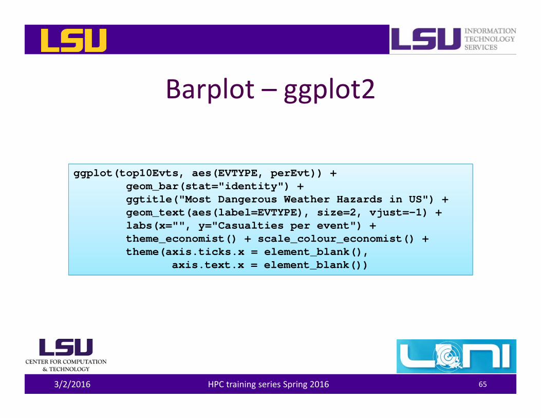
Barplot – ggplot2
3/2/2016 HPC training series Spring 2016 65
ggplot(top10Evts, aes(EVTYPE, perEvt)) +geom_bar(stat="identity") +ggtitle("Most Dangerous Weather Hazards in US") +geom_text(aes(label=EVTYPE), size=2, vjust=-1) +labs(x="", y="Casualties per event") +theme_economist() + scale_colour_economist() +theme(axis.ticks.x = element_blank(),
axis.text.x = element_blank())
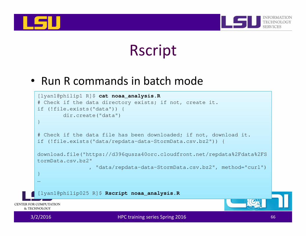
Rscript
• Run R commands in batch mode
3/2/2016 HPC training series Spring 2016 66
[lyan1@philip1 R]$ cat noaa_analysis.R# Check if the data directory exists; if not, create it.if (!file.exists("data")) {
dir.create("data")}
# Check if the data file has been downloaded; if not, download it.if (!file.exists("data/repdata-data-StormData.csv.bz2")) {
download.file("https://d396qusza40orc.cloudfront.net/repdata%2Fdata%2FStormData.csv.bz2"
, "data/repdata-data-StormData.csv.bz2", method="curl")}…
[lyan1@philip025 R]$ Rscript noaa_analysis.R
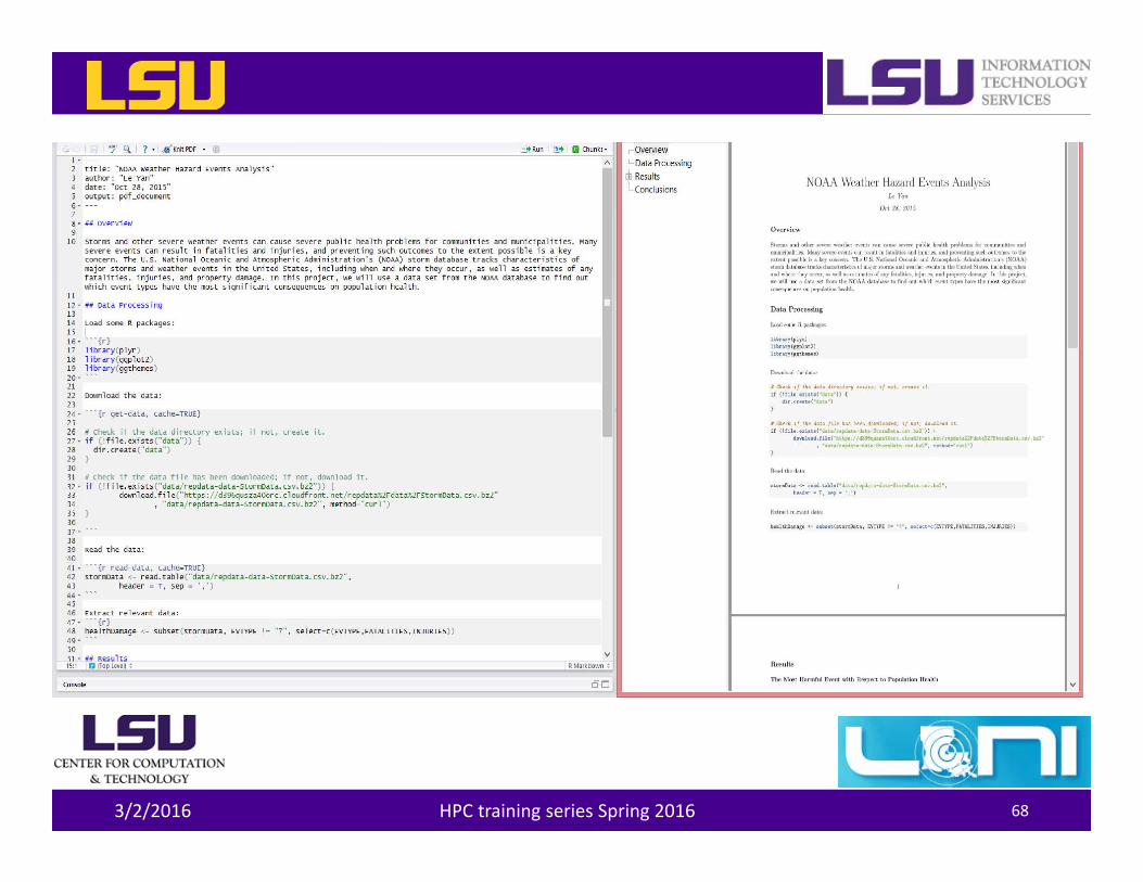
Data Analysis with Reporting
• knitr is a R package that allows one to generate dynamic report by weaving R code and human readable texts together– It uses the markdown syntax– The output can be HTML, PDF or (even) Word
3/2/2016 HPC training series Spring 2016 67
3/2/2016 HPC training series Spring 2016 68
Not Covered
• Statistical analysis (e.g regression models, machine learning/data mining)
• Profiling and debugging• …• Chances are that R has something in store for you whenever it comes to data analysis
3/2/2016 HPC training series Spring 2016 69
Learning R• User documentation on CRAN
– An Introduction on R: http://cran.r‐project.org/doc/manuals/r‐release/R‐intro.html
• Online tutorials– http://www.cyclismo.org/tutorial/R/
• Online courses (e.g. Coursera)• Educational R packages
– Swirl: Learn R in R
3/2/2016 HPC training series Spring 2016 70

Next Tutorial – Introduction to Python
• This training will provide a brief introduction to the python programming language, introduce you to some useful python modules for system management and scientific computing.
• Date: March 9th, 2016
3/2/2016 HPC training series Spring 2016 71

Getting Help• User Guides
– LSU HPC: http://www.hpc.lsu.edu/docs/guides.php#hpc– LONI:http://www.hpc.lsu.edu/docs/guides.php#loni
• Documentation: http://www.hpc.lsu.edu/docs• Online courses: http://moodle.hpc.lsu.edu• Contact us
– Email ticket system: sys‐[email protected]– Telephone Help Desk: 225‐578‐0900– Instant Messenger (AIM, Yahoo Messenger, Google Talk)
• Add “lsuhpchelp”
3/2/2016 HPC training series Spring 2016 72

Questions?
3/2/2016 HPC training series Spring 2016 73