Embed Size (px)
Citation preview
Introduction to Rfor Absolute Beginners: Part I
Melinda FrickeDepartment of Linguistics
University of California, Berkeley
D-Lab Workshop Series, Spring 2013
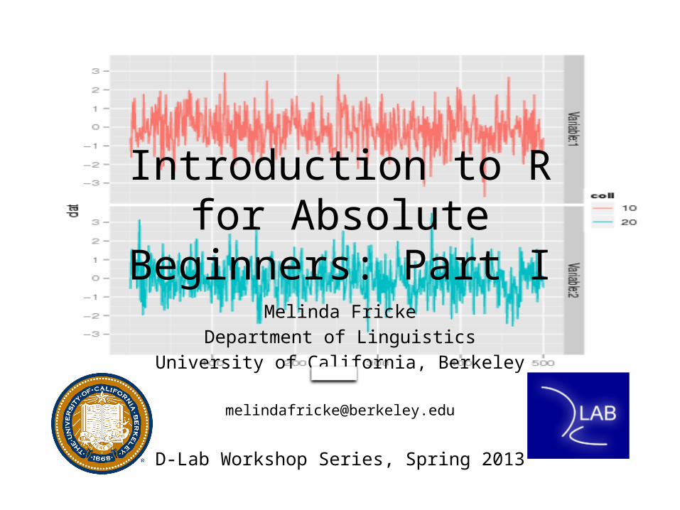
Why this workshop?
"The questions that statistical analysis is designed to answer can often be stated simply. This may encourage the layperson to believe that the answers are similarly simple. Often, they are not…
No-one should be embarrassed that they have difficulty with analyses that involve ideas that professional statisticians may take 7 or 8 years of professional training and experience to master.”
(Maindonald and Braun, 2010. Data Analysis and Graphics Using R: An Example-Based Approach.)
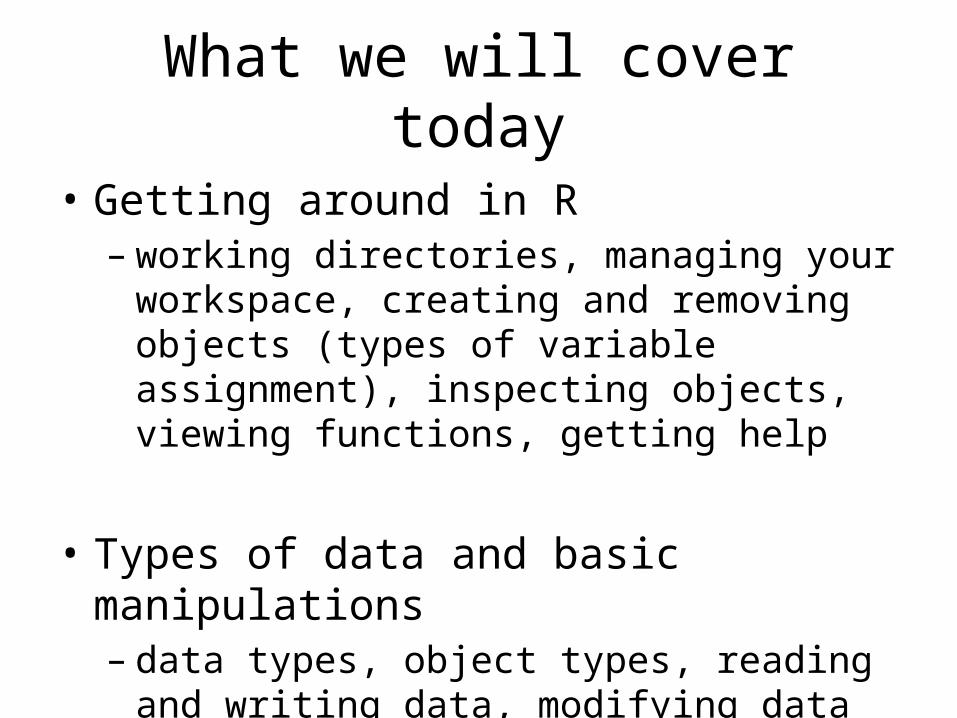
What we will cover today
• Getting around in R– working directories, managing your workspace,
creating and removing objects (types of variable assignment), inspecting objects, viewing functions, getting help
• Types of data and basic manipulations– data types, object types, reading and writing data,
modifying data and objects, basic functions
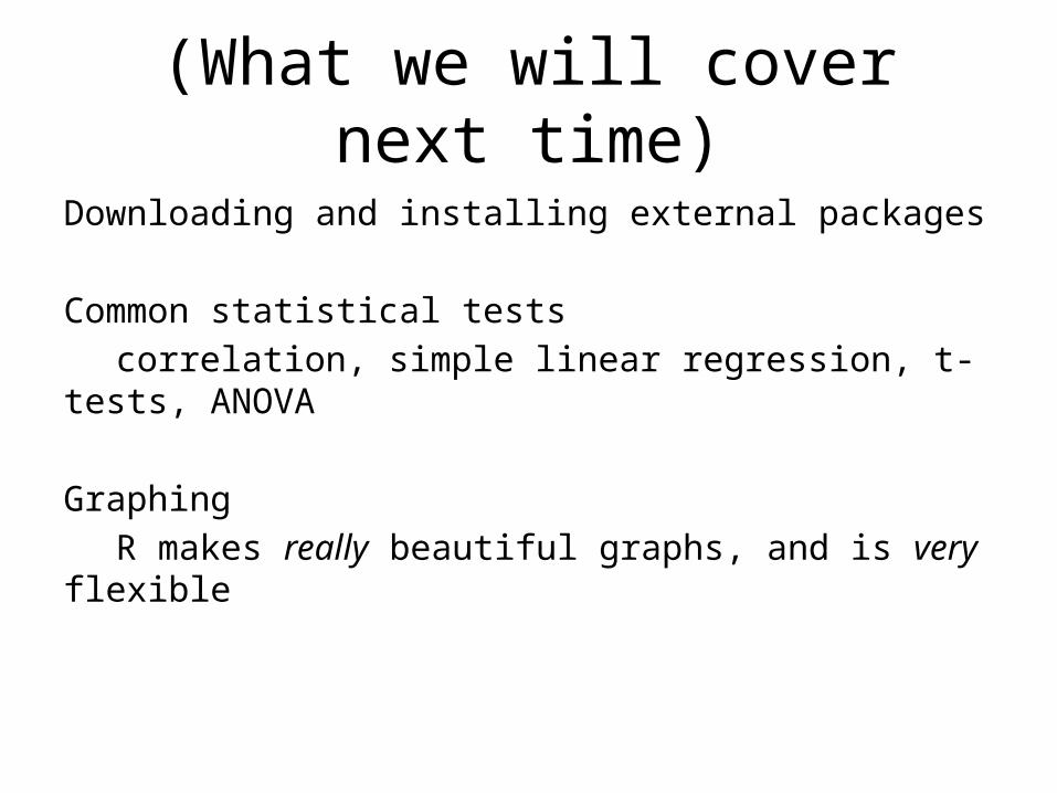
(What we will cover next time)
Downloading and installing external packages
Common statistical testscorrelation, simple linear regression, t-tests, ANOVA
GraphingR makes really beautiful graphs, and is very flexible

What we will not cover (ever)
"The best any analysis can do is to highlight the information in the data. No amount of statistical or computing technology can be a substitute for good design of data collection, for understanding the context in which data are to be interpreted, or for skill in the use of statistical analysis methodology. Statistical software systems are one of several components of effective data analysis.”
(Maindonald and Braun, 2010)
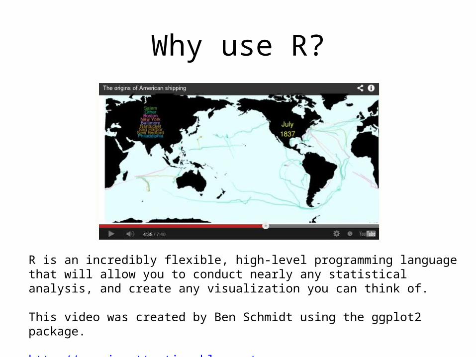
Why use R?
R is an incredibly flexible, high-level programming language that will allow you to conduct nearly any statistical analysis, and create any visualization you can think of.
This video was created by Ben Schmidt using the ggplot2 package.
http://sappingattention.blogspot.com/2012/10/data-narratives-and-structural.html

A simpler example…
(These are from my own work on the production of “s” sounds.)

But first, the basics…
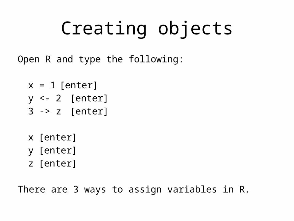
Creating objects
Open R and type the following:
x = 1 [enter]y <- 2 [enter]3 -> z [enter]
x [enter]y [enter]z [enter]
There are 3 ways to assign variables in R.
Creating objects
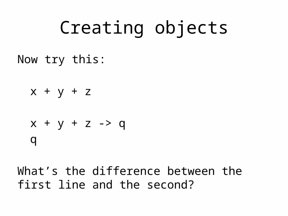
Now try this:
x + y + z
x + y + z -> qq
What’s the difference between the first line and the second?
Creating objects
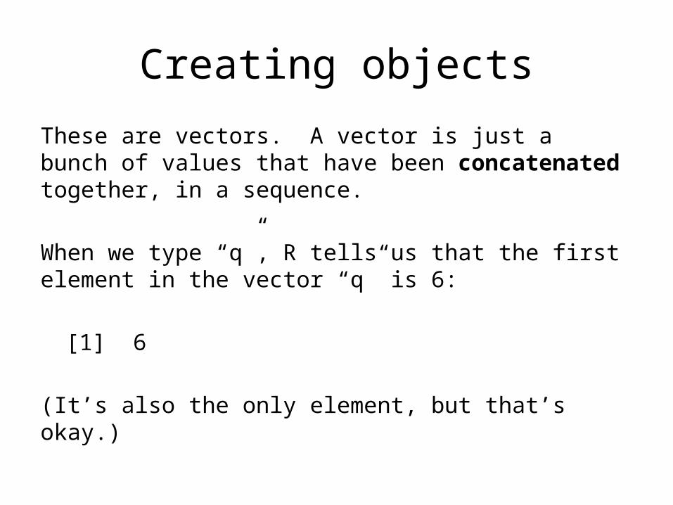
These are vectors. A vector is just a bunch of values that have been concatenated together, in a sequence.
When we type “q”, R tells us that the first element in the vector “q” is 6:
[1] 6
(It’s also the only element, but that’s okay.)
Creating objects
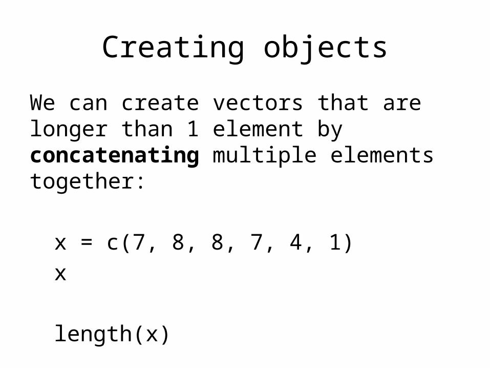
We can create vectors that are longer than 1 element by concatenating multiple elements together:
x = c(7, 8, 8, 7, 4, 1)x
length(x)

A little bit about “looping”
R is a “high level” programming language. This means it takes care of a lot of things for us.
x * 2
x + y
Most programming languages require you to write loops, but R takes care of a lot of “looping” on its own.
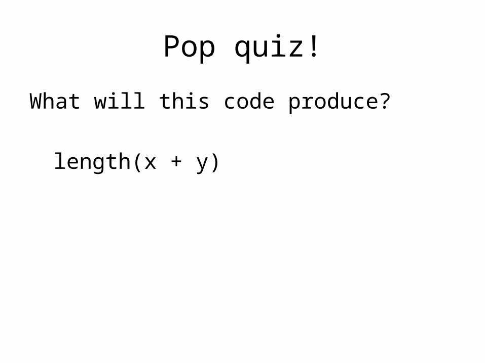
Pop quiz!
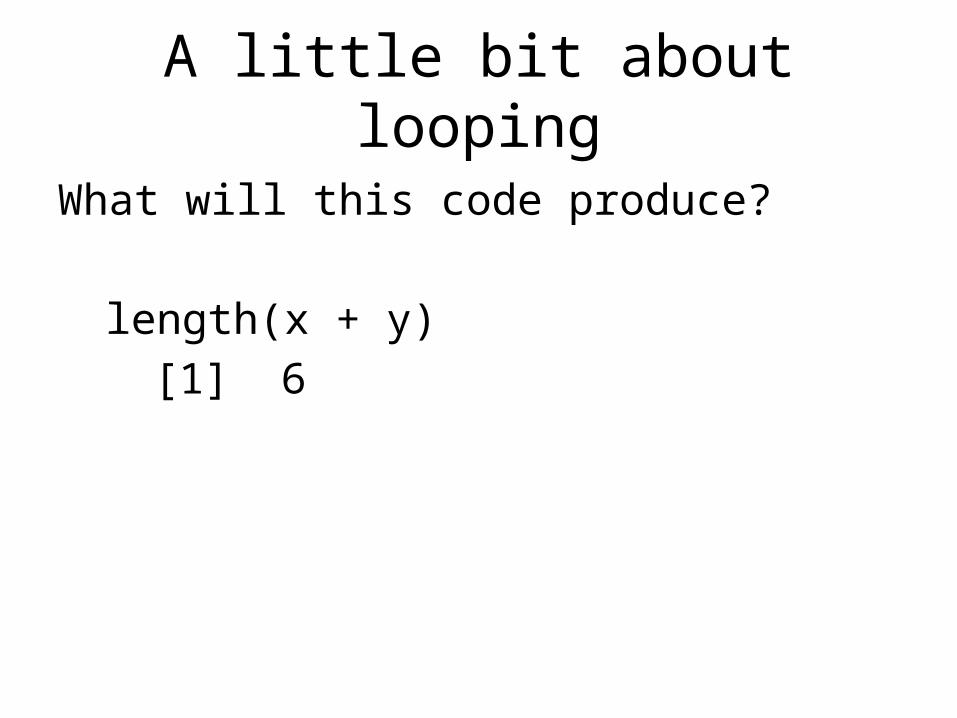
What will this code produce?
length(x + y)
A little bit about looping
What will this code produce?
length(x + y)[1] 6
A little bit about looping
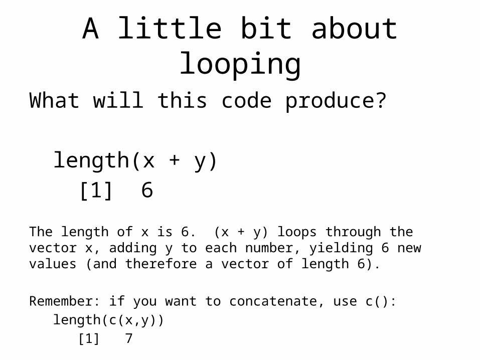
What will this code produce?
length(x + y)[1] 6
The length of x is 6. (x + y) loops through the vector x, adding y to each number, yielding 6 new values (and therefore a vector of length 6).
Remember: if you want to concatenate, use c():length(c(x,y))
[1] 7

Pop quiz!
What will this code produce?
length(x + y)[1] 6
length(length(x + y))

Pop quiz!
What will this code produce?
length(x + y)[1] 6
length(length(x + y))[1] 1
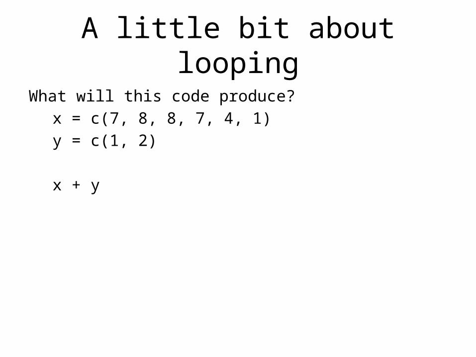
A little bit about looping
What will this code produce?x = c(7, 8, 8, 7, 4, 1)y = c(1, 2)
x + y
A little bit about looping
What will this code produce?x = c(7, 8, 8, 7, 4, 1)y = c(1, 2)
x + y[1] 8 10 9 9 5 3
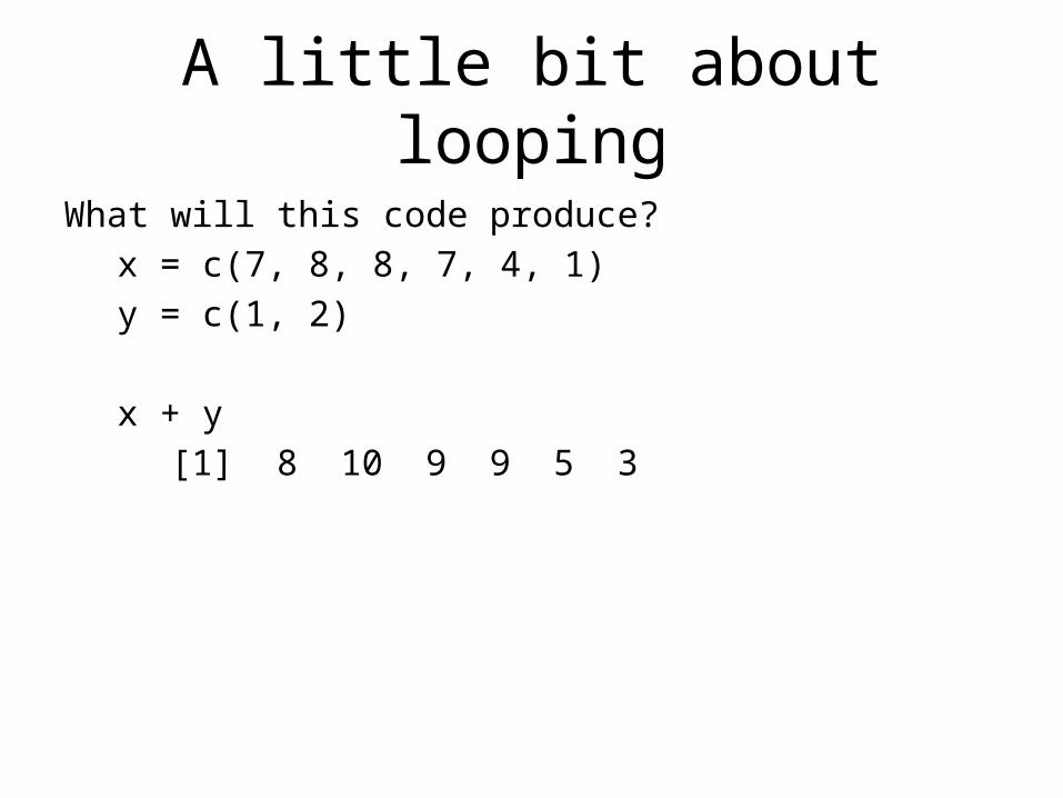
A little bit about looping
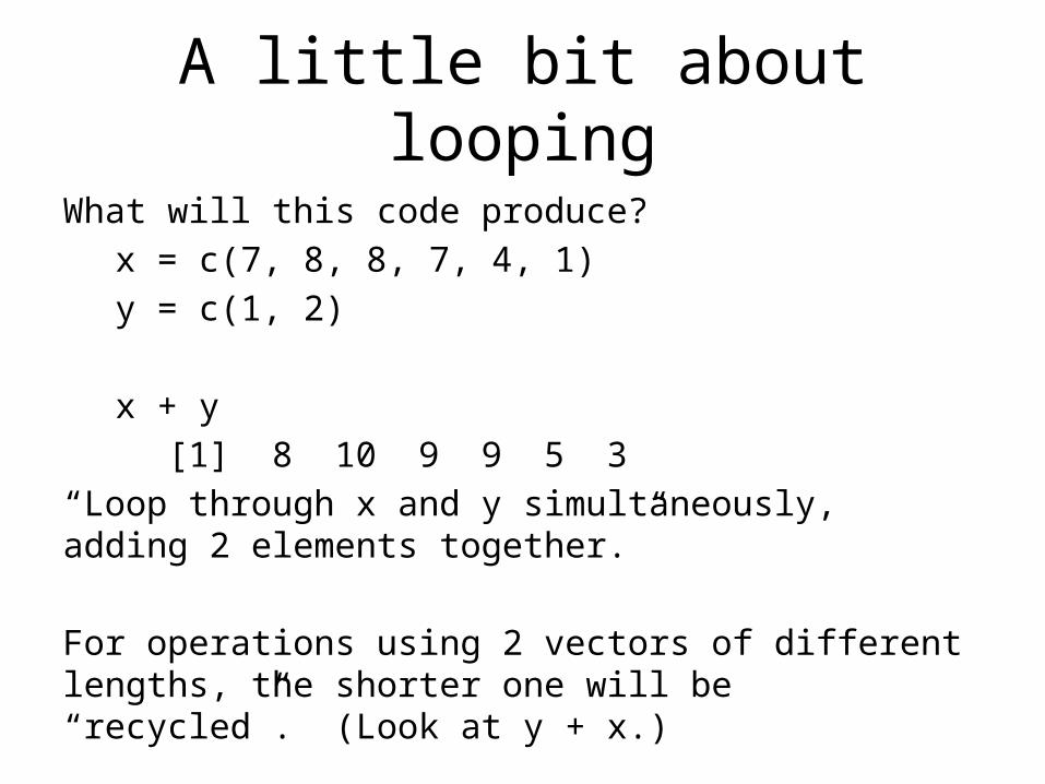
What will this code produce?x = c(7, 8, 8, 7, 4, 1)y = c(1, 2)
x + y[1] 8 10 9 9 5 3
“Loop through x and y simultaneously, adding 2 elements together.”
For operations using 2 vectors of different lengths, the shorter one will be “recycled”. (Look at y + x.)

Data types
class(x)
class(‘x’)
Data types
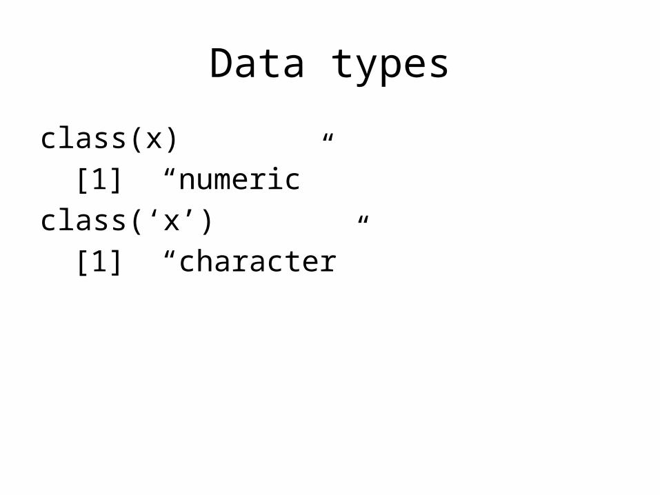
class(x)[1] “numeric”
class(‘x’)[1] “character”
Data types
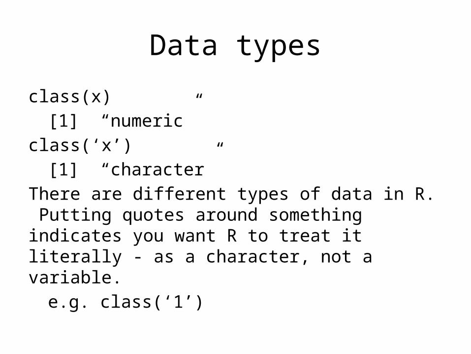
class(x)[1] “numeric”
class(‘x’)[1] “character”
There are different types of data in R. Putting quotes around something indicates you want R to treat it literally - as a character, not a variable.
e.g. class(‘1’)
Data types
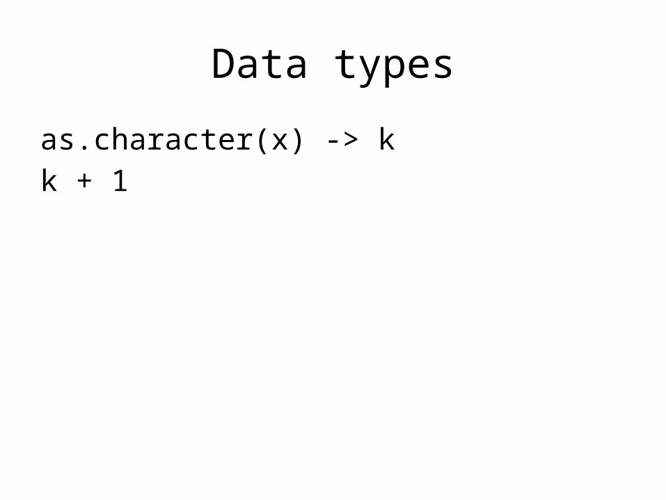
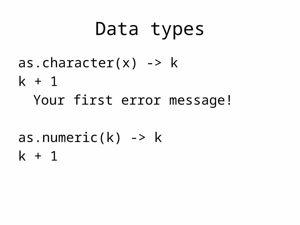
as.character(x) -> kk + 1
Data types
as.character(x) -> kk + 1
Your first error message!
as.numeric(k) -> kk + 1

Data types
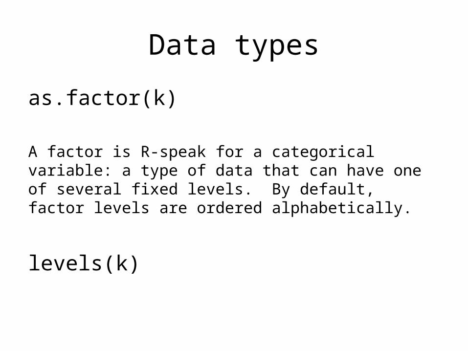
as.factor(k)
Data types
as.factor(k)
A factor is R-speak for a categorical variable: a type of data that can have one of several fixed levels. By default, factor levels are ordered alphabetically.
levels(k)
Data types
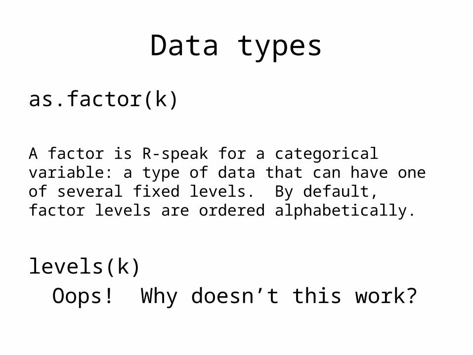
as.factor(k)
A factor is R-speak for a categorical variable: a type of data that can have one of several fixed levels. By default, factor levels are ordered alphabetically.
levels(k)Oops! Why doesn’t this work?
Data types
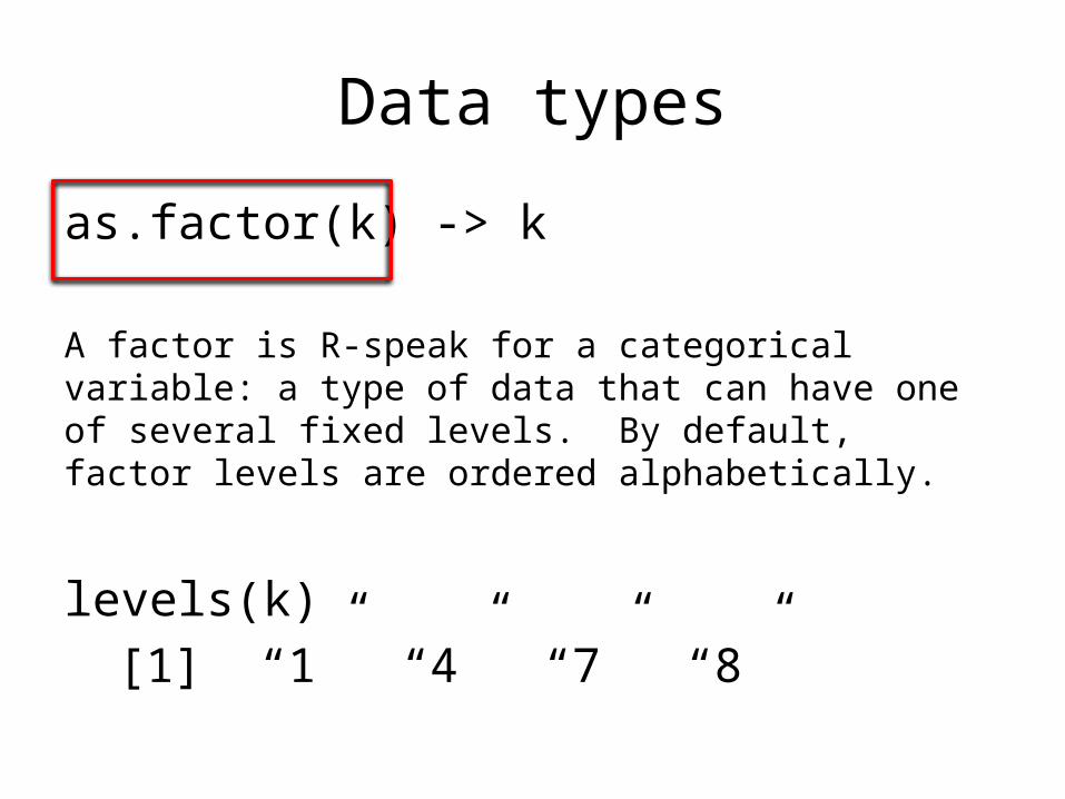
as.factor(k) -> k
A factor is R-speak for a categorical variable: a type of data that can have one of several fixed levels. By default, factor levels are ordered alphabetically.
levels(k)[1] “1” “4” “7” “8”
Data types
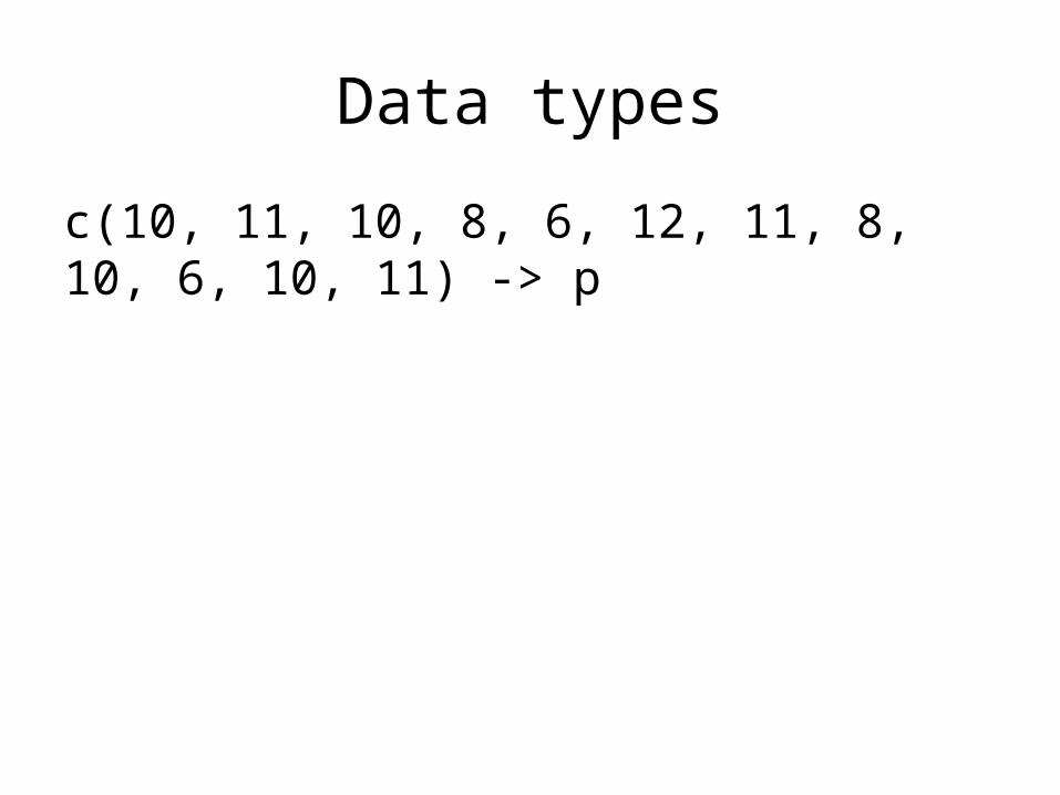
c(10, 11, 10, 8, 6, 12, 11, 8, 10, 6, 10, 11) -> p

Using what we’ve learned so far…
c(10, 11, 10, 8, 6, 12, 11, 8, 10, 6, 10, 11) -> p
How many items are in the vector ‘p’?
How many unique values are in ‘p’?
Using what we’ve learned so far…
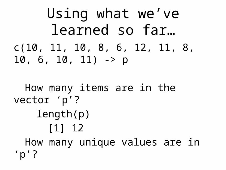
c(10, 11, 10, 8, 6, 12, 11, 8, 10, 6, 10, 11) -> p
How many items are in the vector ‘p’?length(p)
[1] 12How many unique values are in ‘p’?
Using what we’ve learned so far…
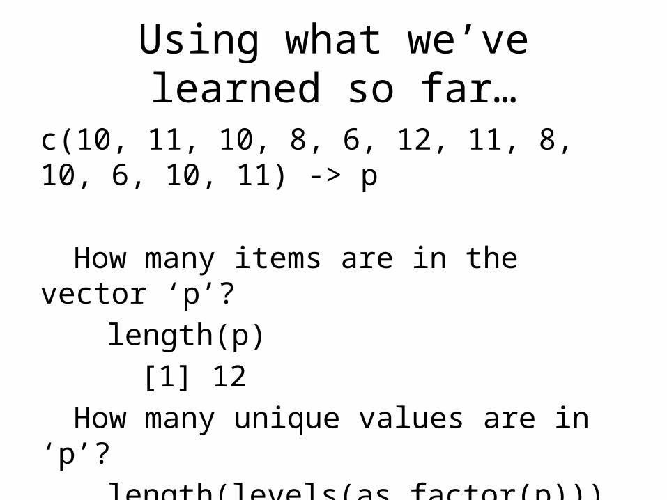
c(10, 11, 10, 8, 6, 12, 11, 8, 10, 6, 10, 11) -> p
How many items are in the vector ‘p’?length(p)
[1] 12How many unique values are in ‘p’?
length(levels(as.factor(p)))
Your first R weirdness
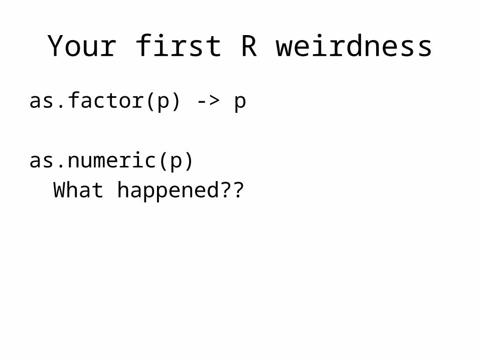
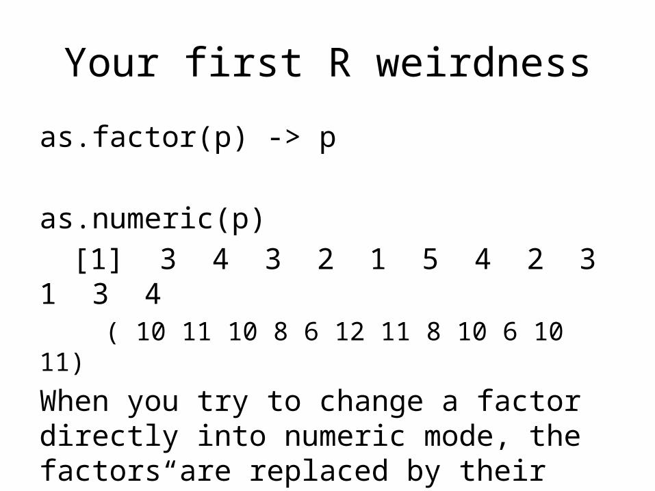
as.factor(p) -> p
as.numeric(p)What happened??
Your first R weirdness
as.factor(p) -> p
as.numeric(p)[1] 3 4 3 2 1 5 4 2 3 1 3 4
( 10 11 10 8 6 12 11 8 10 6 10 11)
When you try to change a factor directly into numeric mode, the factors are replaced by their “order”. How could we avoid this?
Your first R weirdness
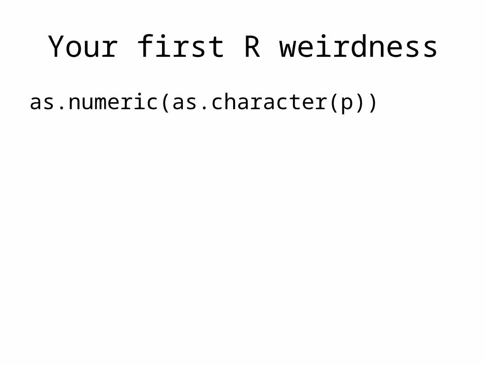
as.numeric(as.character(p))
Your first R weirdness
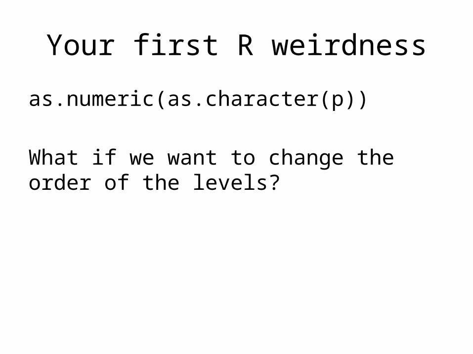
as.numeric(as.character(p))
What if we want to change the order of the levels?
Your first R weirdness
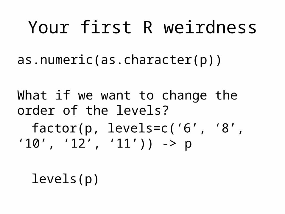
as.numeric(as.character(p))
What if we want to change the order of the levels?
factor(p, levels=c(‘6’, ‘8’, ‘10’, ‘12’, ‘11’)) -> p
levels(p)
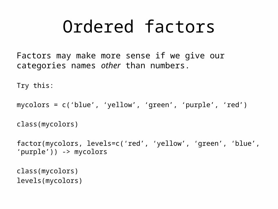
Ordered factors
Factors may make more sense if we give our categories names other than numbers.
Try this:
mycolors = c(‘blue’, ‘yellow’, ‘green’, ‘purple’, ‘red’)
class(mycolors)
factor(mycolors, levels=c(‘red’, ‘yellow’, ‘green’, ‘blue’, ‘purple’)) -> mycolors
class(mycolors)levels(mycolors)
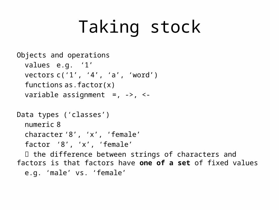
Taking stockObjects and operations
values e.g. ‘1’vectors c(‘1’, ‘4’, ‘a’, ‘word’)functions as.factor(x)variable assignment =, ->, <-
Data types (‘classes’)numeric 8character ‘8’, ‘x’, ‘female’factor ‘8’, ‘x’, ‘female’
the difference between strings of characters and factors is that factors have one of a set of fixed values
e.g. ‘male’ vs. ‘female’

Some more useful functionsType these commands in to see what they do:
ls()table(p)unique(p)sort(p)mean(p)median(p)sd(p)
edit(p)
ls
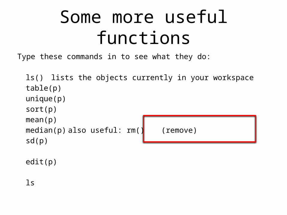
Some more useful functionsType these commands in to see what they do:
ls() lists the objects currently in your workspacetable(p)unique(p)sort(p)mean(p)median(p) also useful: rm() (remove)sd(p)
edit(p)
ls
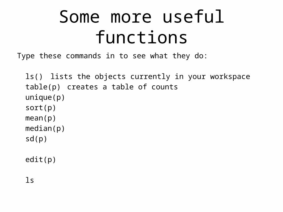
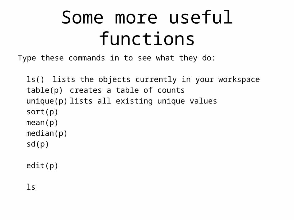
Some more useful functionsType these commands in to see what they do:
ls() lists the objects currently in your workspacetable(p) creates a table of countsunique(p)sort(p)mean(p)median(p)sd(p)
edit(p)
ls
Some more useful functionsType these commands in to see what they do:
ls() lists the objects currently in your workspacetable(p) creates a table of countsunique(p) lists all existing unique valuessort(p)mean(p)median(p)sd(p)
edit(p)
ls
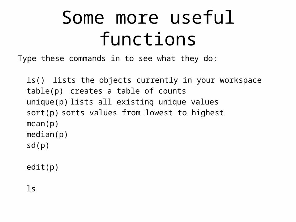
Some more useful functionsType these commands in to see what they do:
ls() lists the objects currently in your workspacetable(p) creates a table of countsunique(p) lists all existing unique valuessort(p) sorts values from lowest to highestmean(p)median(p)sd(p)
edit(p)
ls
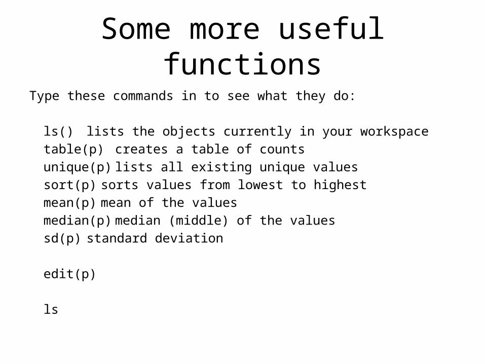
Some more useful functionsType these commands in to see what they do:
ls() lists the objects currently in your workspacetable(p) creates a table of countsunique(p) lists all existing unique valuessort(p) sorts values from lowest to highestmean(p) mean of the valuesmedian(p) median (middle) of the valuessd(p) standard deviation
edit(p)
ls
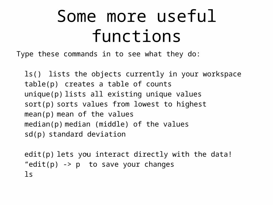
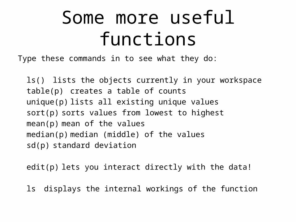
Some more useful functionsType these commands in to see what they do:
ls() lists the objects currently in your workspacetable(p) creates a table of countsunique(p) lists all existing unique valuessort(p) sorts values from lowest to highestmean(p) mean of the valuesmedian(p) median (middle) of the valuessd(p) standard deviation
edit(p) lets you interact directly with the data!“edit(p) -> p” to save your changes
ls
Some more useful functionsType these commands in to see what they do:
ls() lists the objects currently in your workspacetable(p) creates a table of countsunique(p) lists all existing unique valuessort(p) sorts values from lowest to highestmean(p) mean of the valuesmedian(p) median (middle) of the valuessd(p) standard deviation
edit(p) lets you interact directly with the data!
ls displays the internal workings of the function

Getting help with functions
?sort search current packages for a functionhelp(sort) (these two are equivalent)
??sort search all packages for a word
Getting help with functions
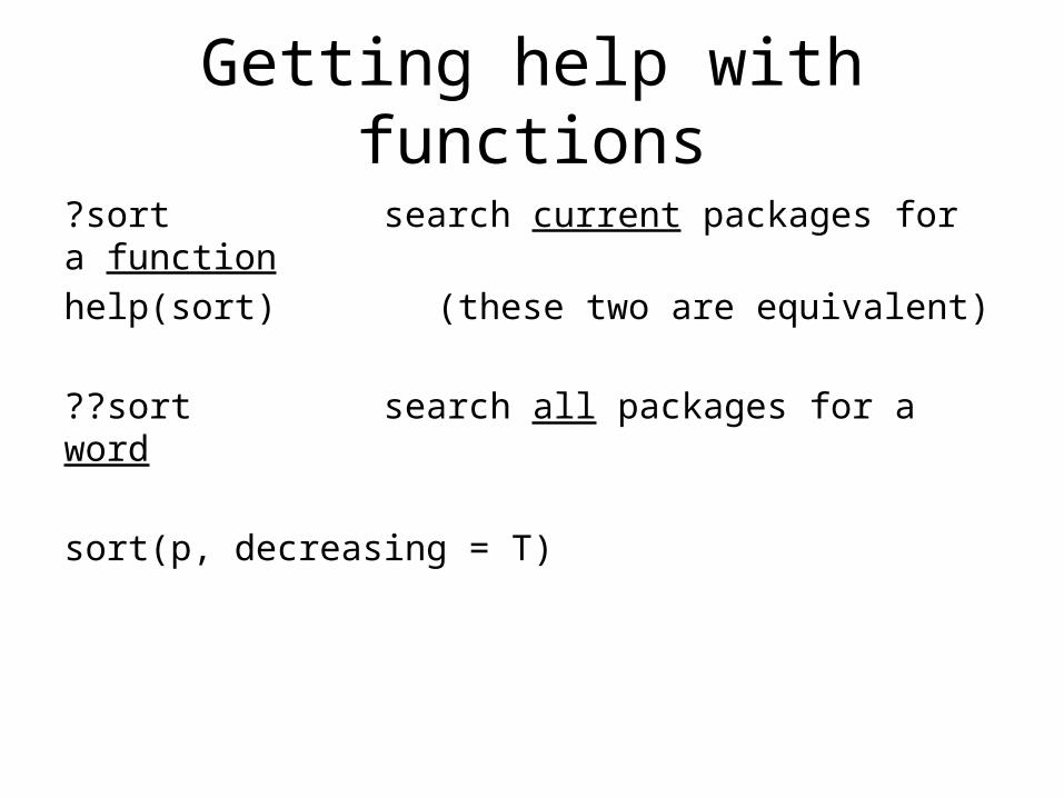
?sort search current packages for a functionhelp(sort) (these two are equivalent)
??sort search all packages for a word
sort(p, decreasing = T)
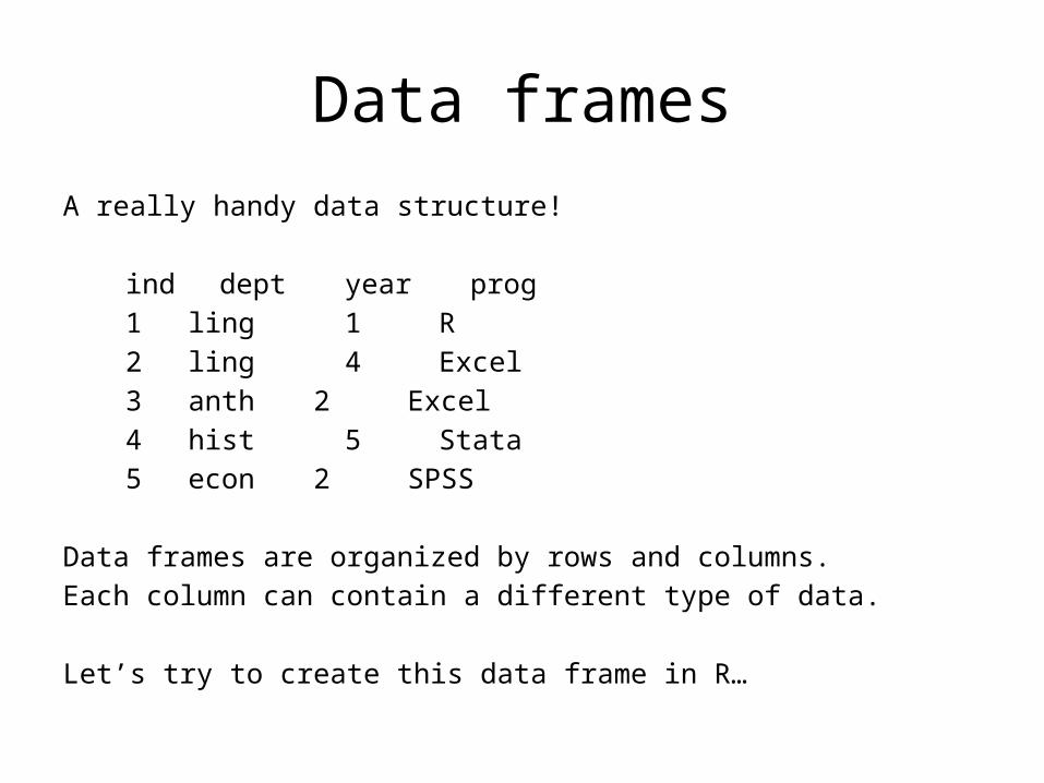
Data framesA really handy data structure!
ind dept year prog1 ling 1 R2 ling 4 Excel3 anth 2 Excel4 hist 5 Stata5 econ 2 SPSS
Data frames are organized by rows and columns.Each column can contain a different type of data.
Let’s try to create this data frame in R…
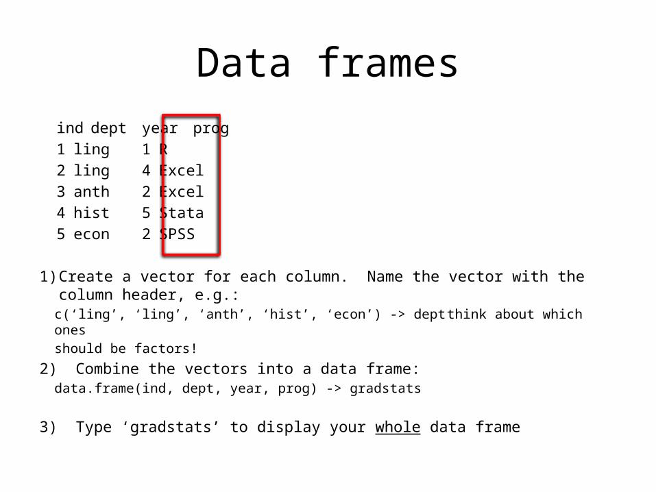
Data framesind dept year prog1 ling 1 R2 ling 4 Excel3 anth 2 Excel4 hist 5 Stata5 econ 2 SPSS
1) Create a vector for each column. Name the vector with the column header, e.g.:c(‘ling’, ‘ling’, ‘anth’, ‘hist’, ‘econ’) -> dept think about which ones
should be factors!
2) Combine the vectors into a data frame:data.frame(ind, dept, year, prog) -> gradstats
3) Type ‘gradstats’ to display your whole data frame
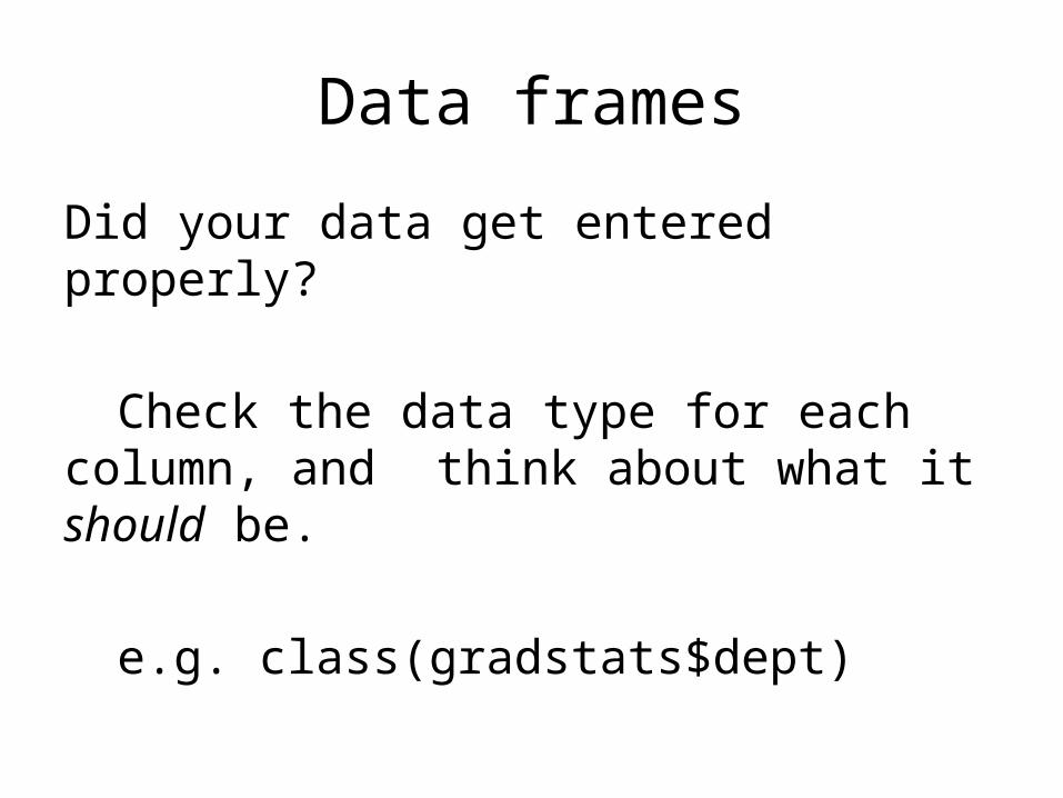
Data frames
Did your data get entered properly?
Check the data type for each column, and think about what it should be.
e.g. class(gradstats$dept)
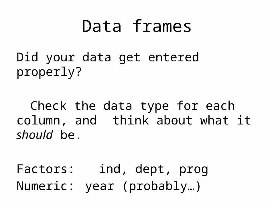
Data frames
Did your data get entered properly?
Check the data type for each column, and think about what it should be.
Factors: ind, dept, progNumeric: year (probably…)
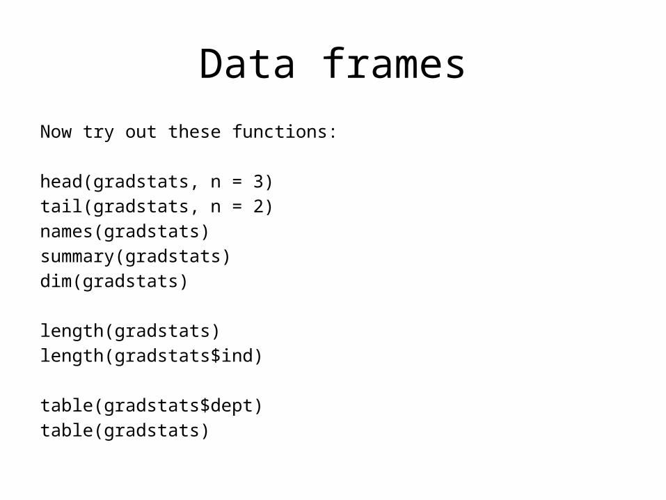
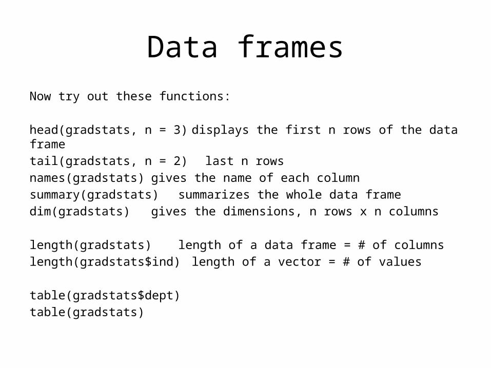
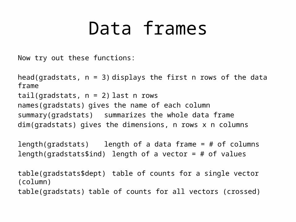
Data framesNow try out these functions:
head(gradstats, n = 3)tail(gradstats, n = 2)names(gradstats)summary(gradstats)dim(gradstats)
length(gradstats)length(gradstats$ind)
table(gradstats$dept)table(gradstats)
Data framesNow try out these functions:
head(gradstats, n = 3) displays the first n rows of the data frametail(gradstats, n = 2) last n rowsnames(gradstats) gives the name of each columnsummary(gradstats) summarizes the whole data framedim(gradstats) gives the dimensions, n rows x n columns
length(gradstats)length(gradstats$ind)
table(gradstats$dept)table(gradstats)
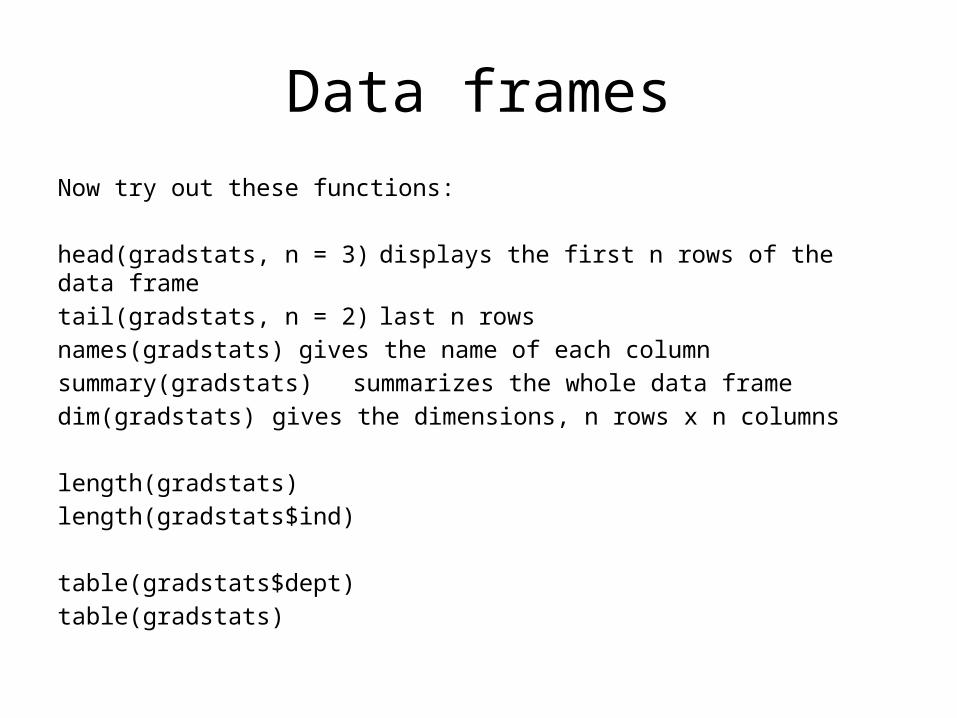
Data framesNow try out these functions:
head(gradstats, n = 3) displays the first n rows of the data frametail(gradstats, n = 2) last n rowsnames(gradstats) gives the name of each columnsummary(gradstats) summarizes the whole data framedim(gradstats) gives the dimensions, n rows x n columns
length(gradstats) length of a data frame = # of columnslength(gradstats$ind) length of a vector = # of values
table(gradstats$dept)table(gradstats)
Data framesNow try out these functions:
head(gradstats, n = 3) displays the first n rows of the data frametail(gradstats, n = 2) last n rowsnames(gradstats) gives the name of each columnsummary(gradstats) summarizes the whole data framedim(gradstats) gives the dimensions, n rows x n columns
length(gradstats) length of a data frame = # of columnslength(gradstats$ind) length of a vector = # of values
table(gradstats$dept) table of counts for a single vector (column)table(gradstats) table of counts for all vectors (crossed)
Data frames
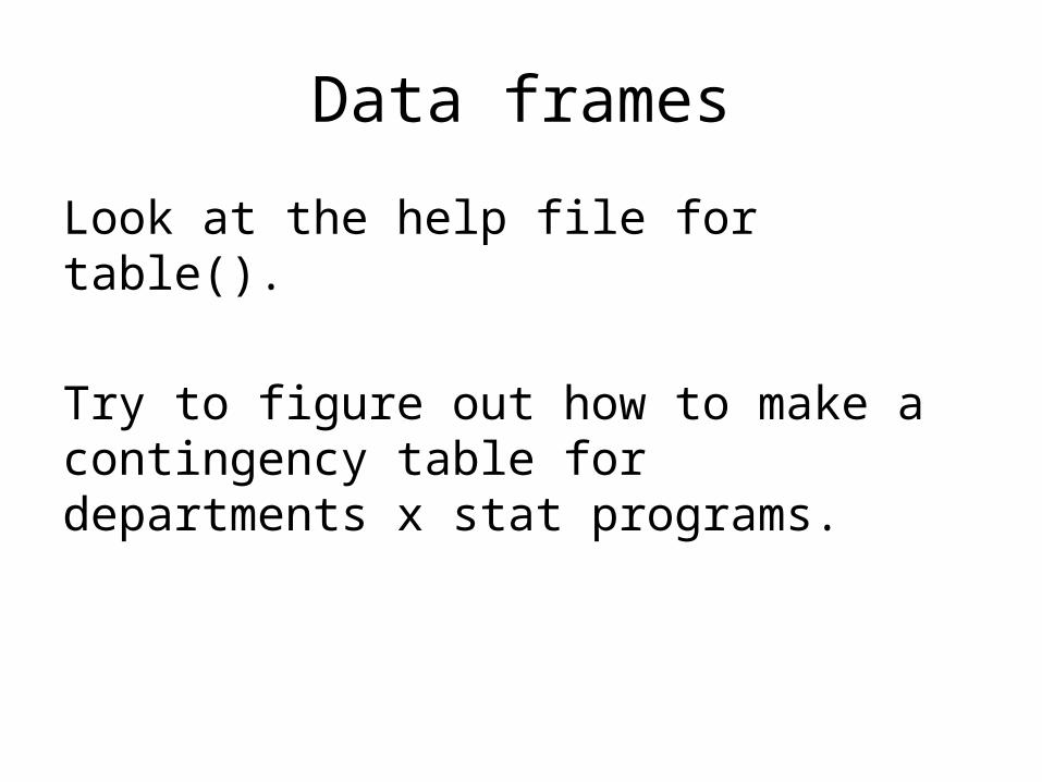
Look at the help file for table().
Try to figure out how to make a contingency table for departments x stat programs.
Data frames
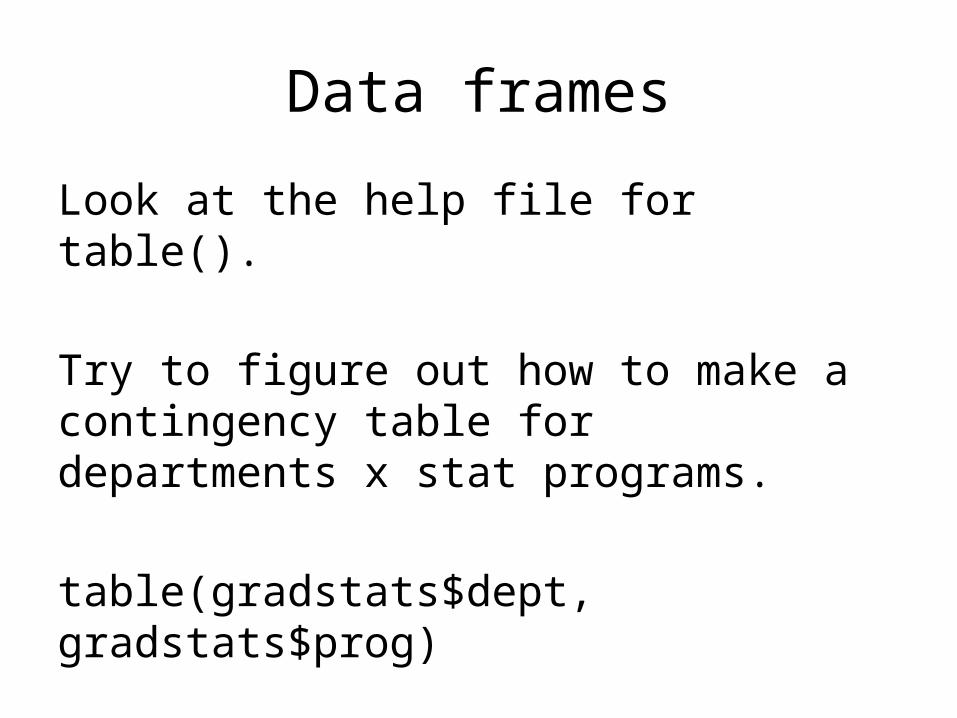
Look at the help file for table().
Try to figure out how to make a contingency table for departments x stat programs.
table(gradstats$dept, gradstats$prog)
Reading in data
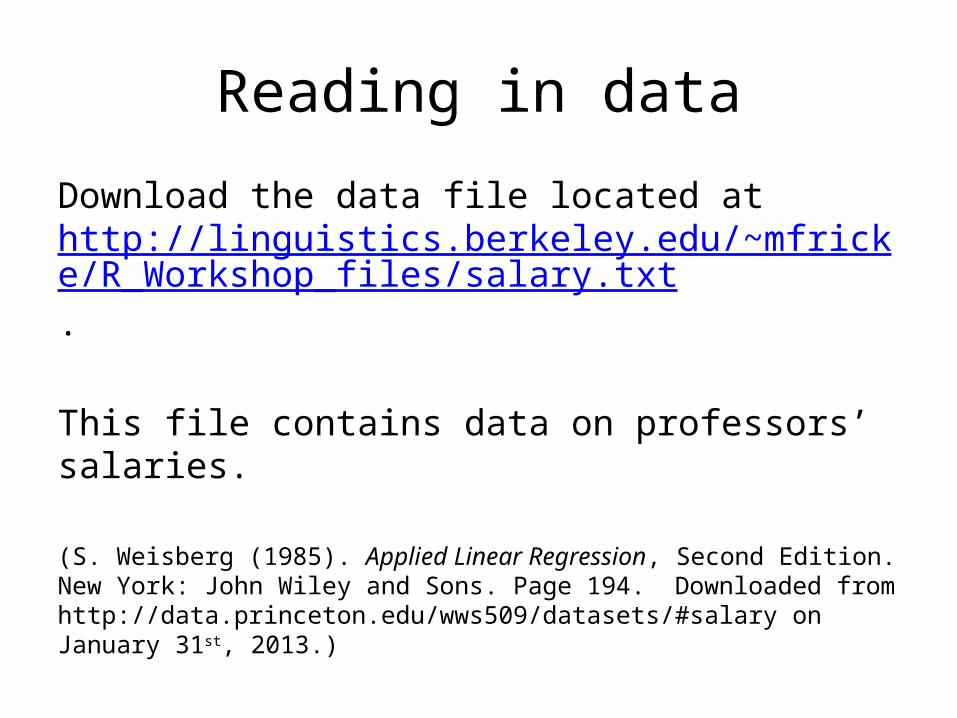
Download the data file located at http://linguistics.berkeley.edu/~mfricke/R_Workshop_files/salary.txt.
This file contains data on professors’ salaries.
(S. Weisberg (1985). Applied Linear Regression, Second Edition. New York: John Wiley and Sons. Page 194. Downloaded from http://data.princeton.edu/wws509/datasets/#salary on January 31st, 2013.)

Reading in data: working directoryYour working directory is where R looks for (and saves) files.
Check to see what it is by typing:
getwd()
You can change it to the directory where you saved the data file with:
setwd()
setwd(“/Users/melindafricke/Desktop”)
But there’s an easier way:On a Mac: command + d, then select your directory.In Windows: go to “File”, then “Change dir…”, and select your directory.
Reading in data
Open the help file for
read.table()
See if you can read in the data file we just downloaded and start inspecting it…
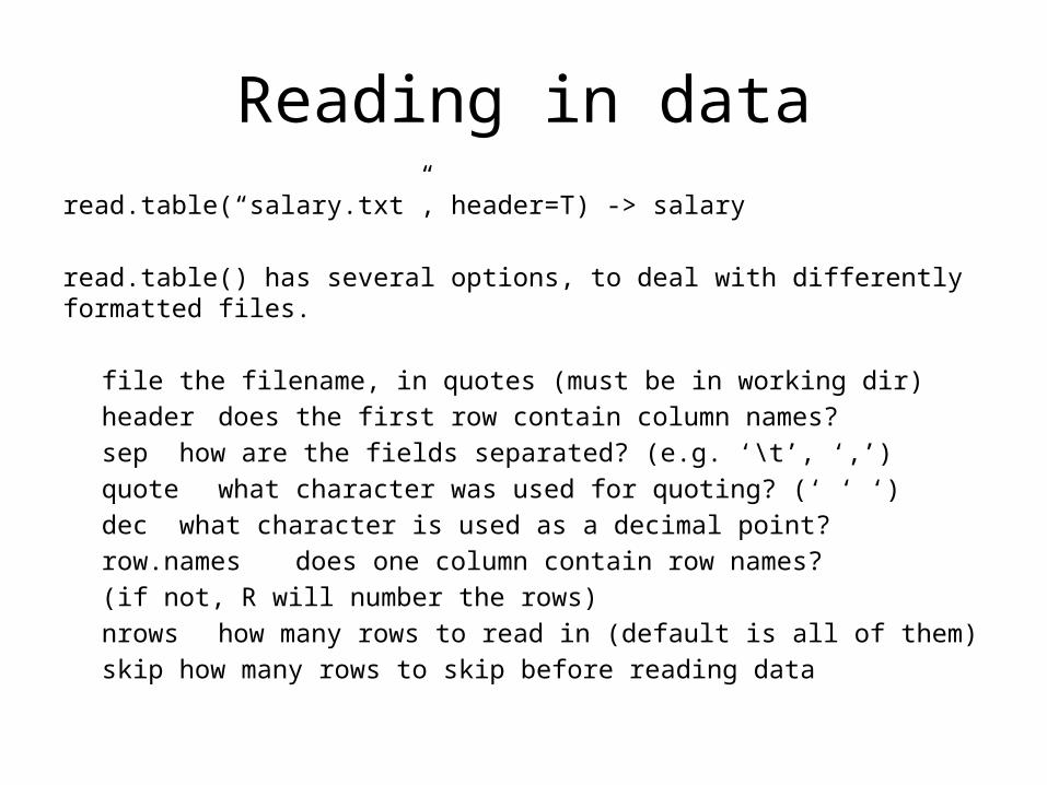
Reading in dataread.table(“salary.txt”, header=T) -> salary
read.table() has several options, to deal with differently formatted files.
file the filename, in quotes (must be in working dir)header does the first row contain column names?sep how are the fields separated? (e.g. ‘\t’, ‘,’)quote what character was used for quoting? (‘ ‘ ‘)dec what character is used as a decimal point?row.names does one column contain row names?
(if not, R will number the rows)nrows how many rows to read in (default is all of them)skip how many rows to skip before reading data
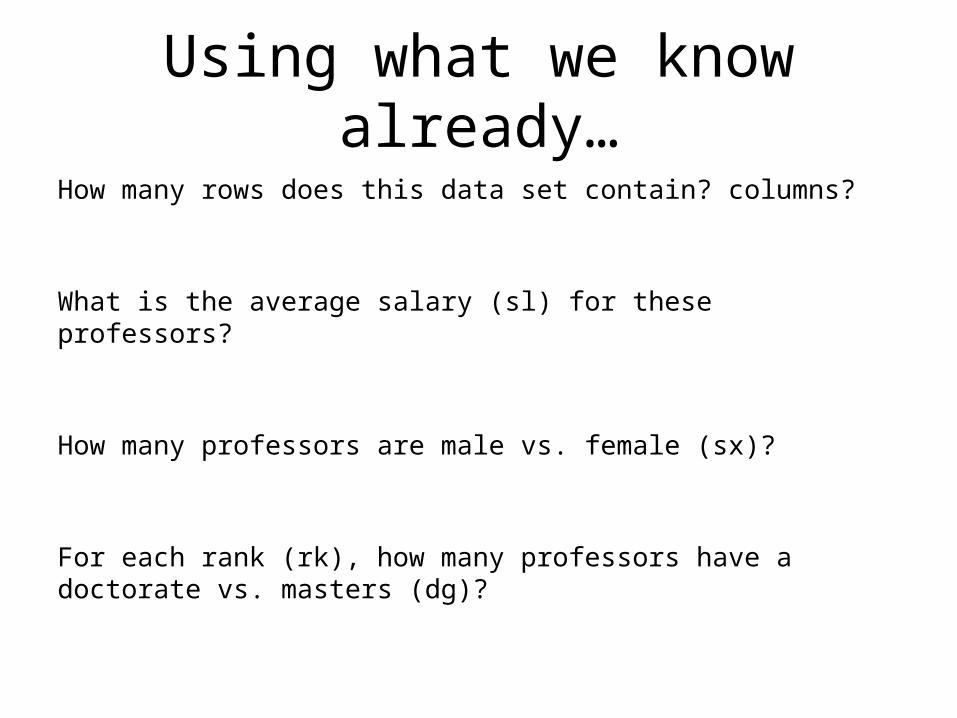
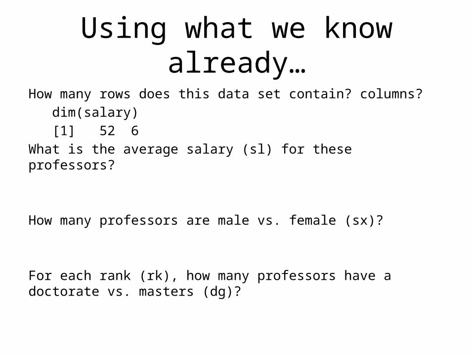
Using what we know already…How many rows does this data set contain? columns?
What is the average salary (sl) for these professors?
How many professors are male vs. female (sx)?
For each rank (rk), how many professors have a doctorate vs. masters (dg)?
Using what we know already…How many rows does this data set contain? columns?
dim(salary)[1] 52 6
What is the average salary (sl) for these professors?
How many professors are male vs. female (sx)?
For each rank (rk), how many professors have a doctorate vs. masters (dg)?
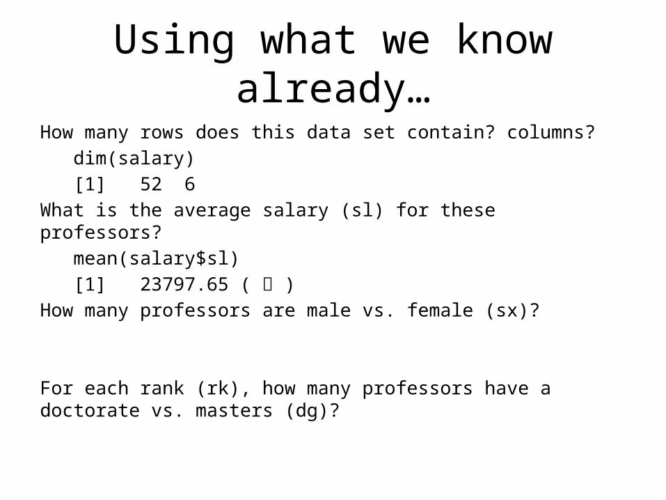
Using what we know already…How many rows does this data set contain? columns?
dim(salary)[1] 52 6
What is the average salary (sl) for these professors?mean(salary$sl)[1] 23797.65 ( )
How many professors are male vs. female (sx)?
For each rank (rk), how many professors have a doctorate vs. masters (dg)?
Using what we know already…How many rows does this data set contain? columns?
dim(salary)[1] 52 6
What is the average salary (sl) for these professors?mean(salary$sl)[1] 23797.65
How many professors are male vs. female (sx)?table(salary$sx) female male
1438
For each rank (rk), how many professors have a doctorate vs. masters (dg)?

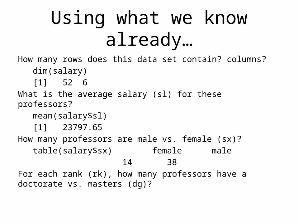
Using what we know already…How many rows does this data set contain? columns?
dim(salary)[1] 52 6
What is the average salary (sl) for these professors?mean(salary$sl)[1] 23797.65
How many professors are male vs. female (sx)?table(salary$sx) female male
14 38For each rank (rk), how many professors have a doctorate vs. masters (dg)?
table(salary$rk, salary$dg) doctorate mastersassistant 14 4associate 5 9full 15 5
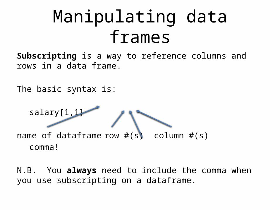
Manipulating data frames
Subscripting is a way to reference columns and rows in a data frame.
The basic syntax is:
salary[1,1]
name of dataframe row #(s) column #(s)comma!
N.B. You always need to include the comma when you use subscripting on a dataframe.
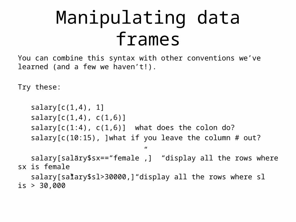
Manipulating data framesYou can combine this syntax with other conventions we’ve learned (and a few we haven’t!).
Try these:
salary[c(1,4), 1]salary[c(1,4), c(1,6)]salary[c(1:4), c(1,6)] what does the colon do?salary[c(10:15), ] what if you leave the column #
out?
salary[salary$sx==“female”,] “display all the rows where sx is female”salary[salary$sl>30000,] “display all the rows where sl is >
30,000”
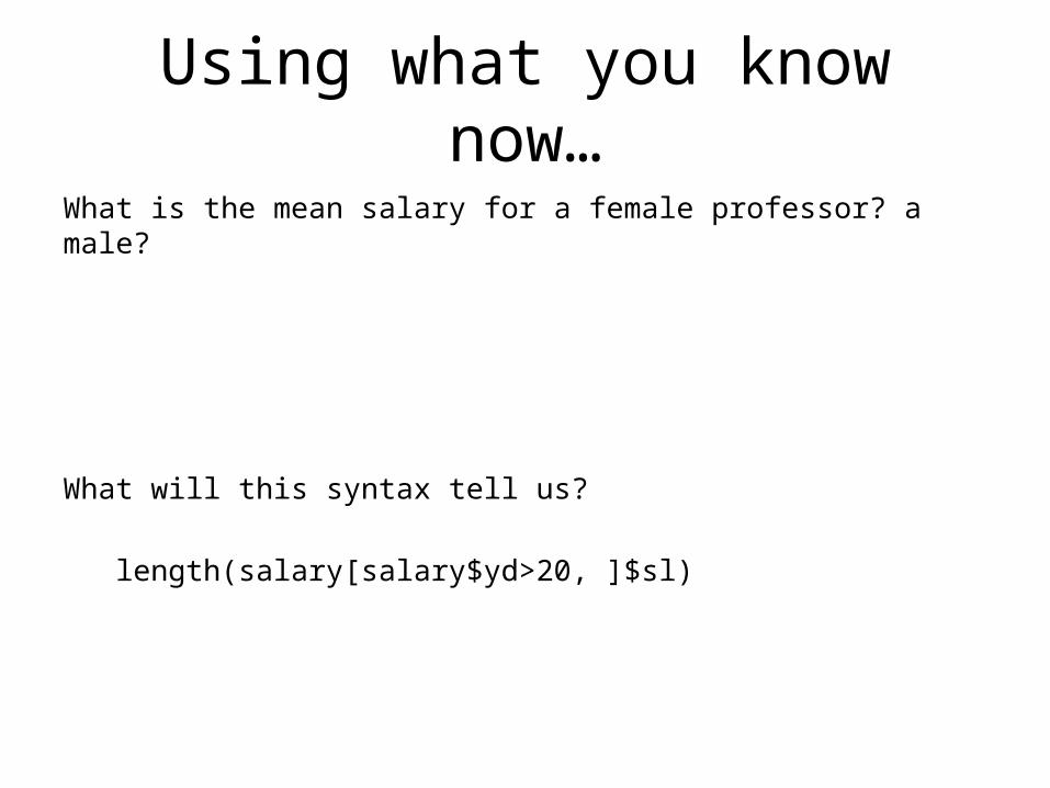
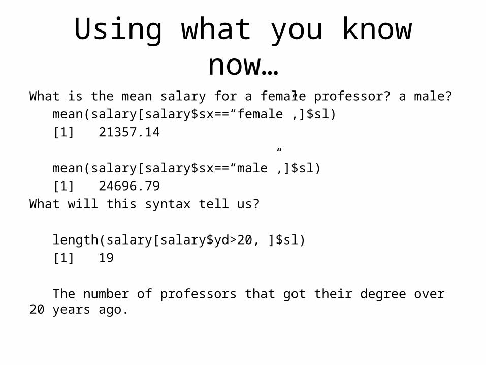
Using what you know now…What is the mean salary for a female professor? a male?
What will this syntax tell us?
length(salary[salary$yd>20, ]$sl)
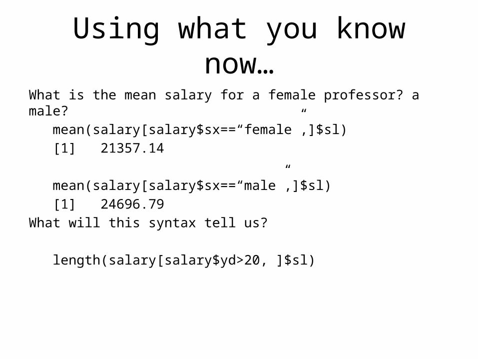
Using what you know now…What is the mean salary for a female professor? a male?
mean(salary[salary$sx==“female”,]$sl)[1] 21357.14
mean(salary[salary$sx==“male”,]$sl)[1] 24696.79
What will this syntax tell us?
length(salary[salary$yd>20, ]$sl)
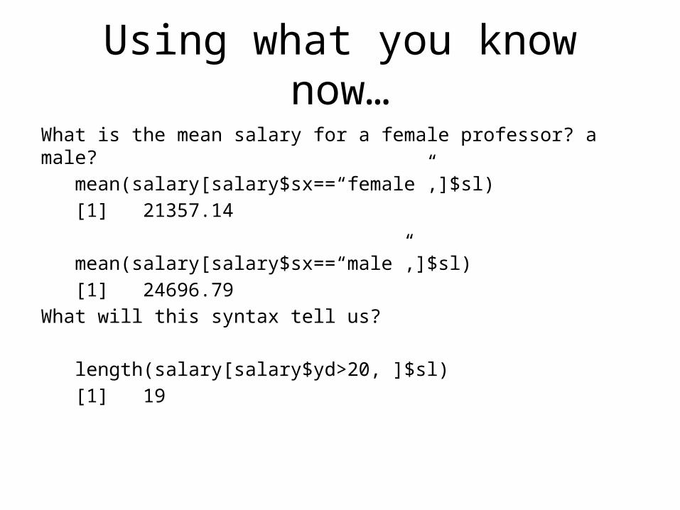
Using what you know now…What is the mean salary for a female professor? a male?
mean(salary[salary$sx==“female”,]$sl)[1] 21357.14
mean(salary[salary$sx==“male”,]$sl)[1] 24696.79
What will this syntax tell us?
length(salary[salary$yd>20, ]$sl)[1] 19
Using what you know now…What is the mean salary for a female professor? a male?
mean(salary[salary$sx==“female”,]$sl)[1] 21357.14
mean(salary[salary$sx==“male”,]$sl)[1] 24696.79
What will this syntax tell us?
length(salary[salary$yd>20, ]$sl)[1] 19
The number of professors that got their degree over 20 years ago.
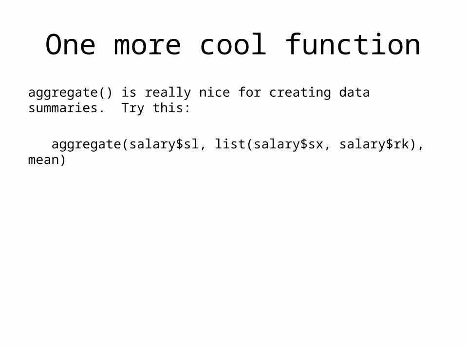
One more cool functionaggregate() is really nice for creating data summaries. Try this:
aggregate(salary$sl, list(salary$sx, salary$rk), mean)
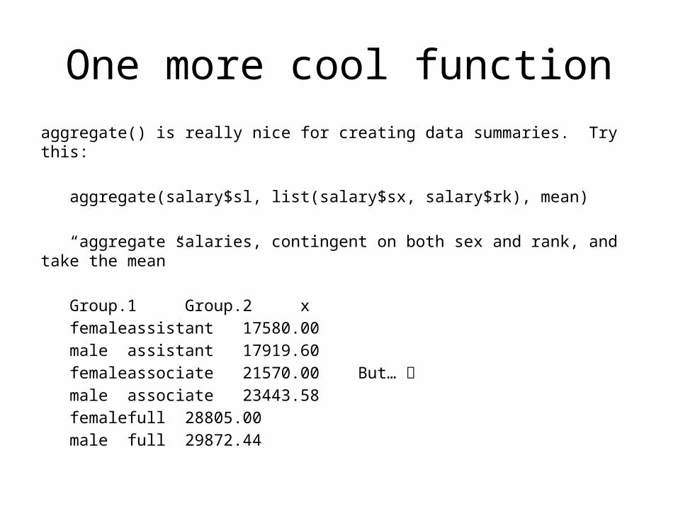
One more cool functionaggregate() is really nice for creating data summaries. Try this:
aggregate(salary$sl, list(salary$sx, salary$rk), mean)
“aggregate salaries, contingent on both sex and rank, and take the mean”
Group.1 Group.2 xfemale assistant 17580.00male assistant 17919.60female associate 21570.00 But… male associate 23443.58female full 28805.00male full 29872.44

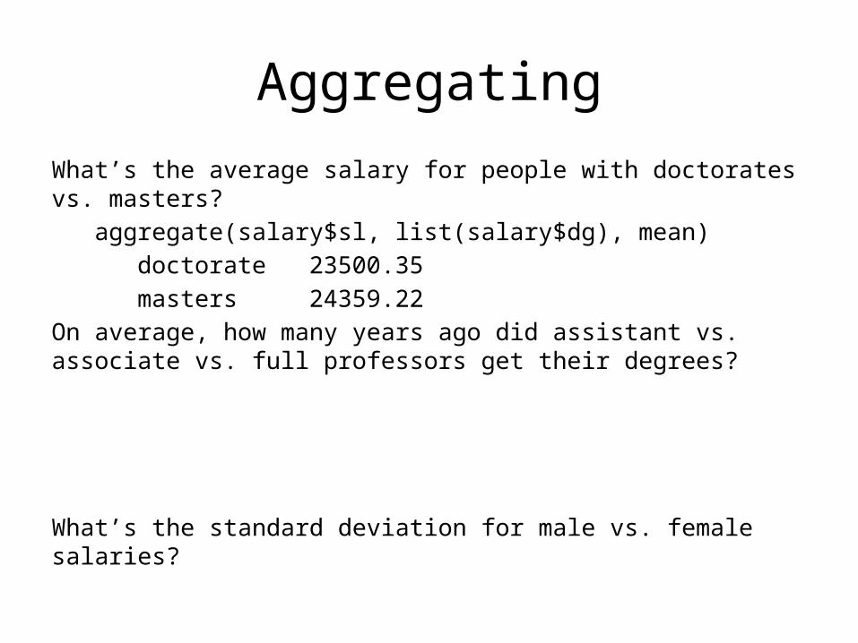
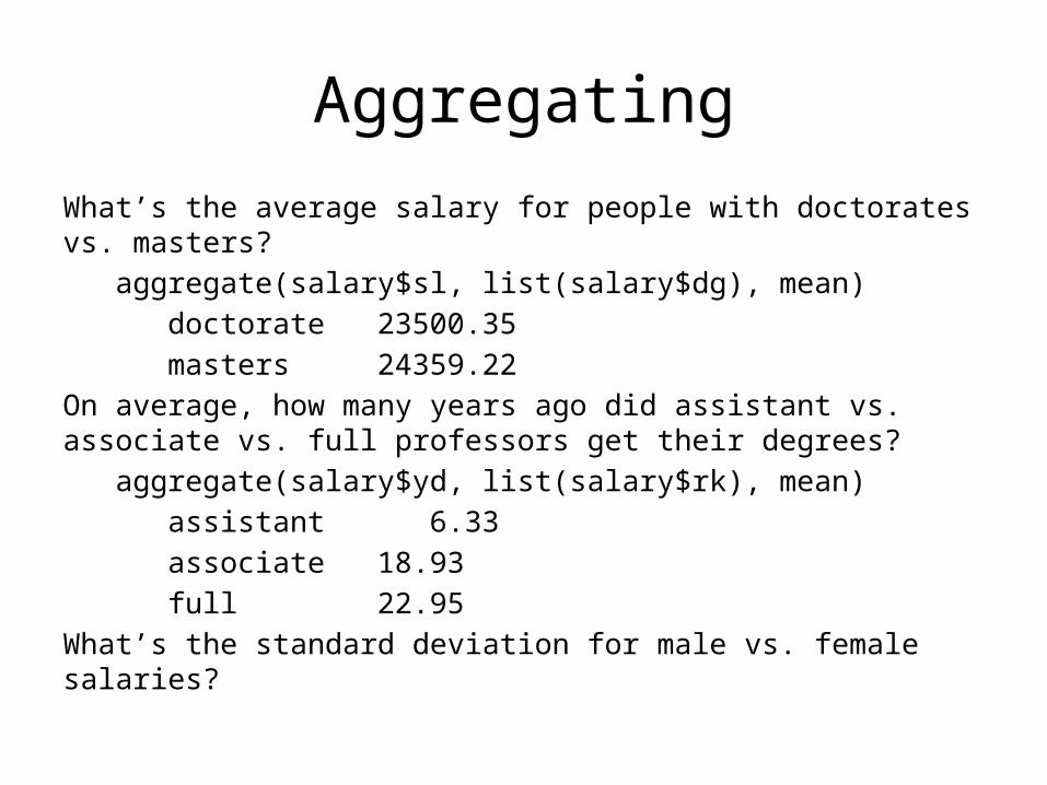
AggregatingWhat’s the average salary for people with doctorates vs. masters?
On average, how many years ago did assistant vs. associate vs. full professors get their degrees?
What’s the standard deviation for male vs. female salaries?
AggregatingWhat’s the average salary for people with doctorates vs. masters?
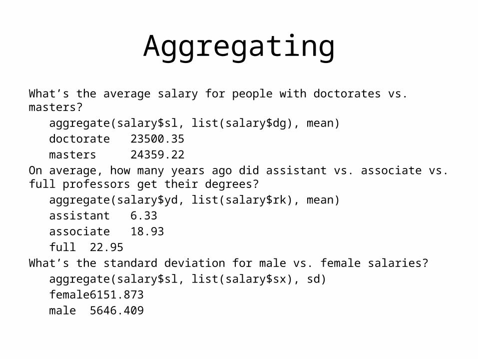
aggregate(salary$sl, list(salary$dg), mean)doctorate 23500.35masters 24359.22
On average, how many years ago did assistant vs. associate vs. full professors get their degrees?
What’s the standard deviation for male vs. female salaries?
AggregatingWhat’s the average salary for people with doctorates vs. masters?
aggregate(salary$sl, list(salary$dg), mean)doctorate 23500.35masters 24359.22
On average, how many years ago did assistant vs. associate vs. full professors get their degrees?
aggregate(salary$yd, list(salary$rk), mean)assistant 6.33associate 18.93full 22.95
What’s the standard deviation for male vs. female salaries?aggregate(salary$sl, list(salary$sx), sd)female 6151.873male 5646.409
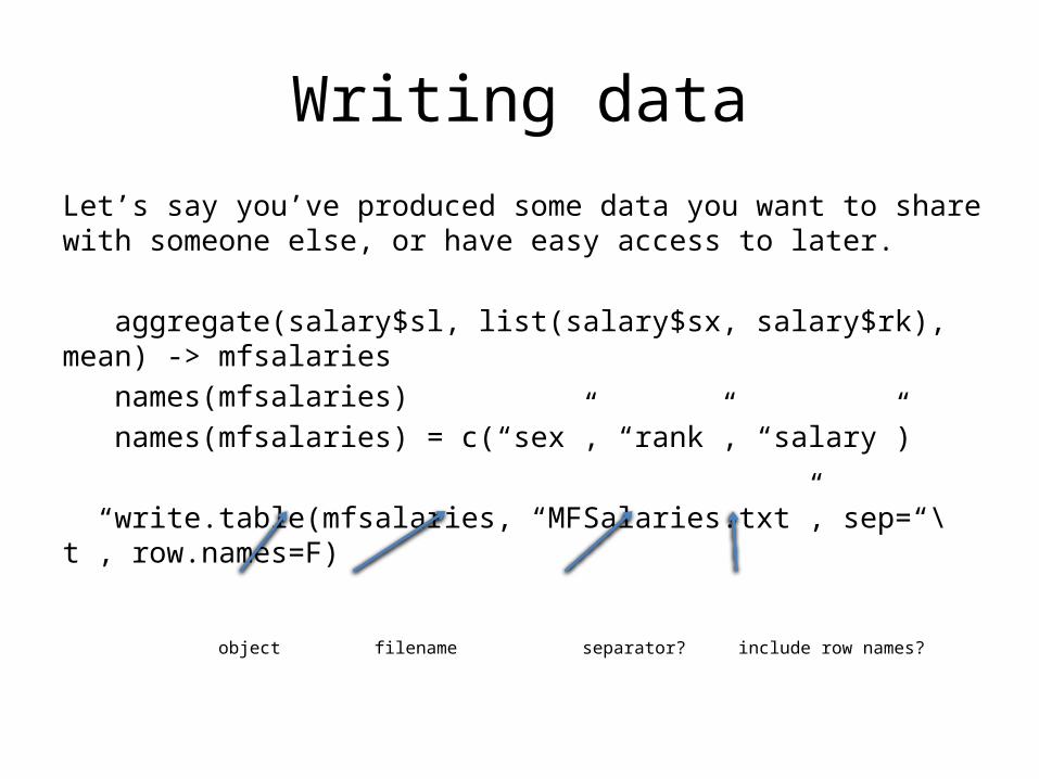
Writing dataLet’s say you’ve produced some data you want to share with someone else, or have easy access to later.
aggregate(salary$sl, list(salary$sx, salary$rk), mean) -> mfsalariesnames(mfsalaries)names(mfsalaries) = c(“sex”, “rank”, “salary”)
write.table(mfsalaries, “MFSalaries.txt”, sep=“\t”, row.names=F)
object filename separator?include row names?

Saving your workspace
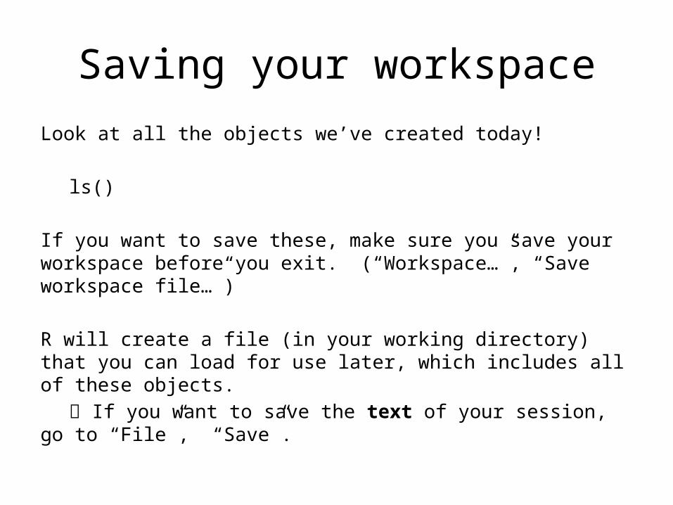
Look at all the objects we’ve created today!
ls()
If you want to save these, make sure you save your workspace before you exit. (“Workspace…”, “Save workspace file…”)
R will create a file (in your working directory) that you can load for use later, which includes all of these objects.
Saving your workspace
Look at all the objects we’ve created today!
ls()
If you want to save these, make sure you save your workspace before you exit. (“Workspace…”, “Save workspace file…”)
R will create a file (in your working directory) that you can load for use later, which includes all of these objects.
If you want to save the text of your session, go to “File”, “Save”.
Next up
Downloading and installing external packages
More sophisticated analysescorrelation, simple linear regression, t-tests, ANOVA
GraphingR makes really beautiful graphs, and is very flexible
Which of these topics are highest priority to you?