Embed Size (px)
Citation preview
Introduction to Quantum Field Theory
for Mathematicians
Lecture notes for Math 273, Stanford, Fall 2018
Sourav Chatterjee
(Based on a forthcoming textbook by Michel Talagrand)


Contents
Lecture 1. Introduction 1
Lecture 2. The postulates of quantum mechanics 5
Lecture 3. Position and momentum operators 9
Lecture 4. Time evolution 13
Lecture 5. Many particle states 19
Lecture 6. Bosonic Fock space 23
Lecture 7. Creation and annihilation operators 27
Lecture 8. Time evolution on Fock space 33
Lecture 9. Special relativity 37
Lecture 10. The mass shell 41
Lecture 11. The postulates of quantum field theory 43
Lecture 12. The massive scalar free field 47
Lecture 13. Introduction to ϕ4 theory 53
Lecture 14. Scattering 57
Lecture 15. The Born approximation 61
Lecture 16. Hamiltonian densities 65
Lecture 17. Wick’s theorem 71
Lecture 18. A first-order calculation in ϕ4 theory 75
Lecture 19. The Feynman propagator 79
Lecture 20. The problem of infinities 83
Lecture 21. One-loop renormalization in ϕ4 theory 87
Lecture 22. A glimpse at two-loop renormalization 93
iii

iv CONTENTS
Lecture 23. The model for free photons 99
Lecture 24. The electromagnetic field 103
Lecture 25. The model for free electrons 107
Lecture 26. The Dirac field 111
Lecture 27. Introduction to quantum electrodynamics 115
Lecture 28. Electron scattering 119
Lecture 29. The Wightman axioms 123

LECTURE 1
Introduction
Date: 9/24/2018Scribe: Andrea Ottolini
1.1. Preview
This course is intended to be an introduction to quantum field theoryfor mathematicians. Although quantum mechanics has been successful inexplaining many microscopic phenomena which appear to be genuinely ran-dom (i.e., the randomness does not stem from the lack of information aboutinitial condition, but it is inherent in the behavior of the particles), it is nota good theory for elementary particles, mainly for two reasons:
• It does not fit well with special relativity, in that the Schrodingerequation is not invariant under Lorentz transformations.• It does not allow creation or annihilation of particles.
Since in lots of interesting phenomena (e.g., in colliders) particles travel atspeeds comparable to the speed of light, and new particles appear after theycollide, these aspects have to be taken into account.
Quantum field theory (QFT) is supposed to describe these phenomenawell, yet its mathematical foundations are shaky or non-existent. The fun-damental objects in quantum field theory are operator-valued distributions.An operator-valued distribution is an abstract object, which when integratedagainst a test function, yields a linear operator on a Hilbert space insteadof a number.
For example, we will define operator-valued distributions a and a† onR3 which satisfy that for all p,p′ ∈ R3,
[a(p), a(p′)] = 0, [a†(p), a†(p′)] = 0,
[a(p), a†(p′)] = (2π)3δ(3)(p− p′)1,
where [A,B] = AB − BA is the commutator, δ(3) is the Dirac δ on R3,and 1 denotes the identity operator on an unspecified Hilbert space. Forsomeone with a traditional training in mathematics, it may not be clearwhat the above statement means. Yet, physics classes on QFT often beginby introducing these operator-valued distributions as if their meaning isself-evident. One of the first objectives of this course is to give rigorousmeanings to a and a†, and define the relevant Hilbert space. It turns out
1
2 1. INTRODUCTION
that the correct Hilbert space is the so-called bosonic Fock space, which wewill define.
Using a and a†, physicists then define the massive scalar free field ϕ withmass parameter m, as
ϕ(t,x) =
∫R3
d3p
(2π)3
1√2ωp
(e−itωp+ix·pa(p) + eitωp−ix·pa†(p)
),
where
ωp =√m2 + |p|2.
Here x · p is the scalar product of x and p, and |p| is the Euclidean normof p. This is an operator-valued distribution defined on spacetime.
Again, it is not at all clear what this means, nor the purpose. We willgive a rigorous meaning to all of these and understand where they comefrom. We will then move on to discuss interacting quantum fields, wherethe Hilbert space is not clear at all, since the Fock space, which does the jobfor the free field, is not going to work. Still, computations can be carriedout, scattering amplitudes can be obtained, and unrigorous QFT theoryleads to remarkably correct predictions for a wide range of phenomena. Wewill talk about all this and more. In particular, we will talk about ϕ4 theory,one-loop renormalization, and the basics of quantum electrodynamics.
1.2. A note on mathematical rigor
Much of quantum field theory is devoid of any rigorous mathematicalfoundation. Therefore we have no option but to abandon mathematicalrigor for large parts of this course. There will be parts where we will notprove theorems with full rigor, but it will be clear that the proofs can bemade mathematically complete if one wishes to do so. These are not theproblematic parts. However, there will be other parts where no one knowshow to put things in a mathematically valid way, and they will appearas flights of fancy to a mathematician. Yet, concrete calculations yieldingactual numbers can be carried out in these fanciful settings, and we willgo ahead and do so. These situations will be pointed out clearly, and willsometimes be posed as open problems.
1.3. Notation
The following are some basic notations and conventions that we willfollow. We will need more notations, which will be introduced in laterlectures.
• Throughout these lectures, we will work in units where ~ = c = 1,where ~ is Planck’s constant divided by 2π and c is the speed oflight.• H is a separable complex Hilbert space.• If a ∈ C, a∗ is its complex conjugate.

1.3. NOTATION 3
• The inner product of f, g ∈ H, denoted by (f, g), is assumed to beantilinear in the first variable and linear in the second. In partic-ular, if en∞n=1 is an orthonormal basis of H, and if f =
∑αnen
and g =∑βnen, then (f, g) =
∑∞n=1 α
∗nβn.
• The norm of a state f is denoted by ‖f‖. A state f is callednormalized if ‖f‖ = 1.• If A is a bounded linear operator on H, A† denotes its adjoint.• If A is a bounded linear operator and A = A†, we will say that A
is Hermitian. We will later replace this with a more general notionof ‘self-adjoint’.• δ is the Dirac delta at 0, and δx is the Dirac delta at x. Among
the properties of the delta function, we will be interested in thefollowing two:∫ ∞
−∞dzδ(x− z)δ(z − y)ξ(z) = δ(x− y)ξ(z),
δ(x) = limε→0
∫R
dy
2πeixy−εy
2=
1
2π
∫Rdy eixy.
• f(p) =∫R dx e
−ixpf(x) is the Fourier transform of f .
Note that some of the definitions are slightly different than the usual math-ematical conventions, such as that of the Fourier transform. Usually, it isjust a difference of sign, but these differences are important to remember.


LECTURE 2
The postulates of quantum mechanics
Date: 9/26/2018Scribe: Sanchit Chaturvedi
2.1. Postulates 1–4
We will introduce our framework of quantum mechanics through a se-quence of five postulates. The first four are given below.
P1 The state of a physical system is described by a vector in a separablecomplex Hilbert space H.
P2 To each (real-valued) observable O corresponds a Hermitian opera-tor A on H. (It can be a bounded linear operator such that A = A†
but not all A will be like this.)P3 If A is the operator for an observable O then any experimentally
observed value of O must be an eigenvalue of A.P4 Suppose that O is an observable with operator A. Suppose further
that A has an orthonormal sequence of eigenvectors xn∞n=1 witheigenvalues λn. Suppose also that the system is in state ψ ∈ H.Then the probability that the observed value of O = λ is given by∑
i:λi=λ|(xi, ψ)|2‖ψ‖2 .
These postulates will be slightly modified later, and replaced with moremathematically satisfactory versions. P5 will be stated later in this lecture.
2.2. A simple example
Consider a particle with two possible spins, say 1 and −1. Then H = C2.Consider the observable
O =
+1, if spin is 1,−1, if spin is −1.
Suppose that we take the operator for this observable to be the matrix
A =
(1 00 −1
)This has eigenvectors (
10
),
(01
)5

6 2. THE POSTULATES OF QUANTUM MECHANICS
with eigenvalues 1,−1. If the state of the system is(α1
α2
)∈ C2,
then
Prob(O = 1) =|α1|2
|α1|2 + |α2|2and
Prob(O = −1) =|α2|2
|α1|2 + |α2|2.
2.3. Adjoints of unbounded operators
Definition 2.1. An unbounded operator A on a Hilbert space H is alinear map from a dense subspace D(A) into H.
Definition 2.2. An unbounded operator is called symmetric if
(x,Ay) = (Ax, y) ∀x, y ∈ D(A).
Take any unbounded operator A with domain D(A). We want to definethe adjoint A†. We first define D(A†) to be the set of all y ∈ H such that
supx∈D(A)
|(y,Ax)|‖x‖ <∞.
Then for y ∈ D(A†) define A†y as follows. Define a linear functional λ :D(A)→ C as
λ(x) = (y,Ax).
Since y ∈ D(A†),
c := supx∈D(A)
|(y,Ax)|‖x‖ <∞.
Thus ∀x, x′ ∈ D(A),
|λ(x)− λ(x′)| = |(y,A(x− x′))| ≤ c‖x− x′‖.This implies that λ extends to a bounded linear functional on H. Hencethere exists unique z such that λ(x) = (z, x). Let A†y := z.
Definition 2.3. A symmetric unbounded operator is called self-adjointif D(A) = D(A†), and A† = A on this subspace.
(In practice we only need to verify D(A†) = D(A), since for any sym-metric operator, D(A) ⊆ D(A†), and A† = A on D(A).)
Definition 2.4. An operator B is called an extension of A if D(A) ⊆D(B) and A = B on D(A).
An example is if A is symmetric then A† is an extension of A.
Definition 2.5. A symmetric operatorA is called essentially self-adjointif it has a unique self-adjoint extension.

2.6. POSTULATE 5 7
2.4. Unitary groups of operators
Definition 2.6. A surjective linear operator U : H → H is called uni-tary if ‖Ux‖ = ‖x‖ ∀x ∈ H.
Definition 2.7. A strongly continuous unitary group (U(t))t∈R is acollection of unitary operators such that
• U(s+ t) = U(s)U(t) ∀s, t ∈ R, and• for any x ∈ H the map t 7→ U(t)x is continuous.
2.5. Stone’s Theorem
There is a one-to-one correspondence between one parameter stronglycontinuous unitary groups of operators on H and self-adjoint operators onH. Given U , the corresponding self-adjoint operator A is defined as
Ax = limt→0
U(t)x− xit
,
with D(A) = x : the above limit exists. (It is conventional to write U(t) =eitA.) Conversely, given any self-adjoint operator A, there is a stronglycontinuous unitary group (U(t))t∈R such that the above relation between Aand U is satisfied on the domain of A.
2.6. Postulate 5
P5 If the system is not affected by external influences then its stateevolves in time as ψt = U(t)ψ for some strongly continuous unitarygroup U that only depends on the system (and not on the state).
By Stone’s theorem there exists a unique self-adjoint operator H such thatU(t) = e−itH . This H is called the ‘Hamiltonian’. The Hamiltonian satisfies
d
dtU(t) = −iHU(t) = −iHe−itH
= −iU(t)H = −ie−itHH.We will use the above relations extensively in the sequel.
Besides the five postulates stated above, there is also a sixth postulateabout collapse of wavefunctions that we will not discuss (or need) in theselectures.


LECTURE 3
Position and momentum operators
Date: 9/26/2018Scribe: Sky Cao
3.1. Looking back at Postulate 4
Suppose that A is a self-adjoint operator for an observable O with anorthonormal sequence of eigenvectors u1, u2, . . . and eigenvalues λ1, λ2, . . ..If the system is in state ψ, Postulate 4 says that the probability that theobserved value of O equals λ is given by∑
i:λi=λ|(ui, ψ)|2‖ψ‖2 .
From this, we get the expected value of O:
Eψ(O) =
∑∞i=1 λi|(ui, ψ)|2‖ψ‖2 =
(ψ,Aψ)
‖ψ‖2 .
Similarly,
Eψ(O2) =
∑∞i=1 λ
2i |(ui, ψ)|2‖ψ‖2 =
(ψ,A2ψ)
‖ψ‖2 ,
and more generally
Eψ(Ok) =(ψ,Akψ)
‖ψ‖2 ∀k.
Even more generally, for any α,
Eψ(eiαO) =(ψ, eiαAψ)
‖ψ‖2 .
In certain situations, eiαA may be defined by Taylor series expansion. Butthis is not required; in general we may use Stone’s theorem to make senseof eiαA.
Now recall that the distribution of a random variable X is completelydetermined by its characteristic function
φ(α) = E(eiαX).
This allows us to arrive at the following.
9

10 3. POSITION AND MOMENTUM OPERATORS
Better version of Postulate 4: Suppose that O is an observable withoperator A. If the system is in state ψ, then the characteristic function ofthis observable at α ∈ R is given by
(ψ, eiαAψ)
‖ψ‖2 .
Similarly, we have better versions of the other postulates by replacing ‘Her-mitian’ with ‘self-adjoint’ everywhere.
3.2. A non-relativistic particle in 1-D space
The Hilbert space is H = L2(R). The first observable is the positionobservable. Its operator is denoted X, defined as
(Xψ)(x) = xψ(x).
The domain of X is
D(X) =
ψ ∈ L2(R) :
∫x2|ψ(x)|2dx <∞
.
It can be verified that X is self-adjoint, and that X does not have an or-thonormal sequence of eigenvectors in L2(R).
In physics, they say that X has ‘improper’ eigenfunctions. The Dirac δat x is an improper eigenfunction with eigenvalue x. That is,
Xδx = xδx.
We may verify this in the sense of distributions. For f a test function, wehave ∫
(Xδx)(y)f(y)dy =
∫yδx(y)f(y)dy = xf(x).
On the other hand, ∫xδx(y)f(y)dy = xf(x).
Thus Xδx = xδx.Now suppose the state is ψ. What is the probability distribution of the
position of the particle? According to our better version of Postulate 4, thecharacteristic function of the position variable at α ∈ R is
(ψ, eiαXψ)
‖ψ‖2 .
It is not hard to show that
(eiαXψ)(x) = eiαxψ(x),
and so the characteristic function is∫eiαx|ψ(x)|2dx∫|ψ(x)|2dx .
3.2. A NON-RELATIVISTIC PARTICLE IN 1-D SPACE 11
Thus the probability density of the position is
|ψ(x)|2∫|ψ(z)|2dz .
The ‘position eigenstates’ are δx, x ∈ R. To make this precise, let us approx-imate δx(y) by
1√2πε
e−(y−x)2/2ε
as ε → 0. This state has p.d.f. of the position proportional to e−(y−x)2/ε.This probability distribution converges to the point mass at x as ε→ 0.
The second observable is the momentum observable. The momentumoperator is given by
Pψ = −i ddxψ,
so notationally,
P = −i ddx.
We may take the domain of P to be
ψ ∈ L2(R) : ψ′ ∈ L2(R),but then P will not be self-adjoint. However, one can show that P is es-sentially self-adjoint, that is, there is a unique extension of P to a largerdomain where it is self-adjoint.
Using a similar procedure as with the position, we may show that theprobability density of the momentum is given by
|ψ(p)|2‖ψ‖2
L2
,
where ψ is the Fourier Transform of ψ. The (improper) momentum eigen-state for momentum p is ψ(x) = eipx, because
Pψ = pψ.
Note that ψ is not in L2(R), but we may approximate
ψ(x) ≈ eipx−εx2
for ε small. The Fourier Transform of this function is
ψ(p′) =
∫e−ip
′xeipxdx = 2πδ(p− p′),
which is proportional to the Dirac delta at p.

LECTURE 4
Time evolution
Date: 10/1/2018Scribe: Jack Lindsey
4.1. Probability density of momentum
Let us continue our discussion about the 1D non-relativistic particle thatwe started in the previous lecture. If the system is in state ψ, then we claimthat the probability density function of the momentum at p ∈ R is
|ψ(p)|2‖ψ‖2
L2
,
where ψ is the Fourier transform of ψ. Although a complete proof usingour version of Postulate 4 takes some work, it is easy to see why this is truefrom the following sketch. First, observe that
P kψ = (−i)k dk
dxkψ.
From this it follows that P kψ(p) = pkψ(p). On the other hand, by Postulate4, the expected value of the kth power of the momentum is
(ψ, P kψ)
‖ψ‖2L2
.
By Parseval’s identity, this equals
(ψ, P kψ)
‖ψ‖2L2
=
∫ ∞−∞
dp pk|ψ(p)|2‖ψ‖2
L2
.
This strongly indicates that the p.d.f. of the momentum is proportional to
|ψ(p)|2. A complete proof would require that we work with characteristicfunctions instead of moments.
4.2. The uncertainty principle
Consider the improper state ψ(x) = δx0(x). The position of a particle
in this state is fully concentrated at x0. However, ψ(p) = e−ipx0 , whichmeans that the momentum of the particle is ‘uniformly distributed on thereal line’ — which does not make mathematical sense, but can be thought ofas an idealization of a very spread out probability distribution. On the other
13

14 4. TIME EVOLUTION
hand, if ψ(x) = eip0x, then the position variable has a similar uniform spread
on the real line, but ψ(p) = δ(p− p0), which means that the momentum isfully concentrated at p0.
The above discussion indicates that it may be impossible to have a statethat localizes both the position and the momentum. Indeed, this is a re-sult that can be proved in great generality, as follows. Consider a generalquantum system. Given an observable O with operator A, it follows fromPostulate 4 that if the system is in state ψ, then the standard deviation ofO is given by √
(ψ,A2ψ)
‖ψ‖2 − (ψ,Aψ)2
‖ψ‖4 .
Let us denote this standard deviation by ∆ψ(A). The following result isknown as the Heisenberg Uncertainty Principle (rigorous statement andproof due to H. Weyl):
Theorem 4.1. For any self-adjoint A and B and any ψ ∈ D(A)∩D(B)such that Aψ ∈ D(B) and Bψ ∈ D(A), we have
∆ψ(A)∆ψ(B) ≥ 1
4|(ψ, [A,B]ψ)|2
where [A,B] = AB −BA.
Proof sketch. Apply the Cauchy–Schwarz inequality, starting fromthe right-hand side and expanding.
4.3. The uncertainty principle for position and momentum
Now let us see what the uncertainty principle gives for the position andmomentum operators in 1D. For any ψ, we have
(XPψ)(x) = X(−iψ′)(x) = −ixψ′(x).
On the other hand,
(PXψ)(x) = −i ddx
(xψ(x)) = −ixψ′(x)− iψ(x).
Putting these together, we see that XP −PX = i ·1, where 1 is the identityoperator. Hence, by the uncertainty principle,
∆ψ(X)∆ψ(P ) ≥ 1
4
for all normalized ψ for which [X,P ]ψ is defined and in L2, in units where~ = 1. For example, this holds for any Schwartz function ψ with L2 normequal to one. Note that this implies that position and momentum cannot besimultaneously localized — the p.d.f. of at least one must have substantialstandard deviation.

4.6. A PARTICLE IN A POTENTIAL 15
4.4. Free evolution in 1D
The evolution of the state of a particle in 1D in the absence of a potential(i.e., free evolution) is governed by the Hamiltonian
H = − 1
2m
d2
dx2,
where m is the mass of the particle. (This is a physical fact, with no mathe-matical justification.) The operator H is essentially self-adjoint, and we willidentify it with its unique self-adjoint extension.
If ψ is the state at time 0 and ψt is the state at time t, then ψt = U(t)ψ =e−itHψ. This implies the Schrodinger equation:
∂ψt∂t
= −iHψt =i
2m
∂2ψt∂x2
.
(Again, recall that we are working in units where ~ = 1.) This equationhas an explicit solution, which we will not write down. It is easy to showusing the explicit form of the solution that for any ψ ∈ L2(R), ‖ψt‖L∞ → 0as t → ∞. So the p.d.f. of the position flattens as t → ∞. In other words,there is no limiting probability distribution for the position of the particle;it spreads out across the whole real line.
4.5. Free evolution of the momentum
Now let us see what happens to the momentum of a free particle in 1D.It is not hard to show, using the Schrodinger equation, that
ψt(p) = e−itp2/2mψ(p).
Thus, |ψt(p)|2 = |ψ(p)|2. Hence the p.d.f. of the momentum is not changingat all. This is what we expect, since the momentum of a free particle shouldnot be changing (although, of course, the randomness of the result of a givenobservation is unexpected from a classical perspective).
4.6. A particle in a potential
Now let us briefly consider particles in the presence of a potential V .The Hamiltonian is now given by
H = − 1
2m
d2
dx2+ V,
where V as an operator is defined as (V ψ)(x) = V (x)ψ(x).When is H is essentially self-adjoint? The answer to this question is not
at all obvious. There are many results in the literature, quite comprehen-sively surveyed in Reed and Simon. For example, one useful result is thefollowing.
Theorem 4.2. The Hamiltonian H is essentially self-adjoint if V =V1 + V2 for some V1 ∈ L2(R) and V2 ∈ L∞(R).
16 4. TIME EVOLUTION
This result does not work for growing potentials. For instance, it doesnot cover the case of a simple harmonic oscillator, where V (x) grows quadrat-ically in x. For such cases, the following result, due to Kato, is helpful.
Theorem 4.3. The Hamiltonian H is essentially self-adjoint if V islocally L2 and V (x) ≥ −V ∗(|x|) for some V ∗ such that V ∗(r) = o(r2) asr →∞.
(Note that in particular if V (x) is locally L2 and lower-bounded by aconstant, then it satisfies the condition.)
4.7. Simple harmonic oscillator
Theorem 4.3 says, for example, that H is essentially self-adjoint if
V (x) =1
2mω2x2.
This is the potential for a simple harmonic oscillator with frequency ω.Moreover, the corresponding Hamiltonian
H = − 1
2m
d2
dx2+
1
2mω2x2
has a complete orthonormal sequence of eigenvectors. For simplicity takem = ω = 1. Then the (orthonormal) eigenvectors are
en(x) = CnHn(x)e−x2/2,
where Cn is the normalization constant, and
Hn(x) = (−1)nex2 dn
dxn(e−x
2)
is the ‘nth physicist’s Hermite polynomial’.
4.8. Bound states
Note that ifH is a Hamiltonian and ψ is an eigenfunction with eigenvalueλ, then the evolution of this eigenfunction under this Hamiltonian is givenby ψt = e−itHψ = e−itλψ. So the p.d.f. of the position does not change overtime.
Physicists call this a ‘bound state’. This means that if you are in thestate, you will not freely move out of it (e.g., the p.d.f. of the positionwill not become more and more flat). If you have a potential which allowsparticles to move out freely, then the Hamiltonian cannot have a completeorthonormal sequence of eigenstates as in the previous example.

4.9. DIRAC NOTATION 17
4.9. Dirac notation
Vectors in a Hilbert space are denoted by |x〉 (these care called ‘ketvectors’). Often, we will write vectors like |0〉 , |1〉 , |2〉 , etc. Physicists willsay, for example, that |λ〉 is an eigenvector with eigenvalue λ. Just likemathematicians would write x1, x2, x3, . . . , physicists write |1〉 , |2〉 , |3〉 , . . ..
We also have ‘bra vectors’: 〈x| is the linear functional taking y 7→ (x, y).With this notation, we have
• 〈x|y〉 is the action of x on y, equal to (x, y).• 〈αx|y〉 = α∗ 〈x|y〉 and 〈x|αy〉 = α 〈x|y〉.• (x,Ay) is written as 〈x|A|y〉. Note that A |y〉 = Ay.
One of the great uses of this notation is the following. Let |1〉 , |2〉 , |3〉 , . . .be an orthonormal basis of H. Then
∑∞i=1 |i〉 〈i| = 1, meaning that( ∞∑
i=1
|i〉 〈i|)|x〉 =
∞∑i=1
|i〉 〈i|x〉 = |x〉 .
This is very useful; often one replaces 1 with such an expression in a deriva-tion. Going even further, on L2(R), a physicist would write that
1
2π
∫ ∞−∞
dp |p〉 〈p| = 1,
where |p〉 (x) = eipx, which is an improper element of L2. The derivation isas follows:(
1
2π
∫ ∞−∞
dp |p〉 〈p|)ψ(x) =
(1
2π
∫ ∞−∞
dp |p〉 〈p|ψ〉)
(x)
=1
2π
∫ ∞−∞
dpψ(p)eipx = ψ(x).

LECTURE 5
Many particle states
Date: 10/3/2018Scribe: Philip Ken-Ka Hwang
5.1. Position and momentum space wavefunctions
Consider a particle with state space H = L2(R). Until now, we haverepresented a state |ψ〉 ∈ H as a function ψ ∈ L2(R). This is called the
position space representation of ψ. We can also identify |ψ〉 with ψ, the
Fourier transform of ψ. The function ψ is called the momentum spacerepresentation of |ψ〉, or simply the momentum wavefunction. Physicists
view ψ and ψ as different representations of the same abstract object |ψ〉.Example 5.1. Consider the improper momentum eigenstate |p0〉 for
p0 ∈ R. The position space representation is the function ψ(x) = eip0x. The
Fourier transform of this function is ψ(p) = 2πδ(p− p0). The function ψ is
the momentum space representation of the state |p0〉. Often ψ is also writtenas ψ if it is clear from the context that we are working in momentum space.
We have seen that if ψ is the position space representative of a freeparticle, then ψ evolves as ψt = e−itHψ, where
H = − 1
2m
d2
dx2.
The momentum space representative ϕ = ψ evolves as ϕt(p) = e−itp2/2mϕ(p).
Furthermore the Hamiltonian on the momentum space is
Hϕ(p) =p2
2mϕ(p).
If we distinguish the two Hamiltonian operators as Hx and Hp, then theyare related as
Hxψ = Hpψ.
Usually, such a distinction is not made.
5.2. Schrodinger and Heisenberg pictures
Let ψ be a normalized state. The state ψ evolves in times as ψt = e−itH .If you have an observable with operator A, then its expected value at timet is 〈ψt|A|ψt〉 = (ψt, Aψt). This is called the Schrodinger picture of time
19

20 5. MANY PARTICLE STATES
evolution of states. The Heisenberg picture is a different way of lookingat time evolution, where operators evolve instead of states. If A is theoperator for an observable, then in the Heisenberg picture, the operator forthe same observable at time t is At = eitHAe−itH . The expected value ofthe observable at time t is just the expected value of At computed at time 0,that is, 〈ψ|At|ψ〉. Note that this gives the same result as in the Schrodingerpicture, since
〈ψ|At|ψ〉 = 〈ψ|eitHAe−itH |ψ〉 = 〈ψt|A|ψt〉.Thus, the two pictures are different ways of carrying out the same calcula-tions. In quantum field theory, however, it often helps to think in terms ofthe Heisenberg picture.
5.3. Tensor product state spaces
Let H be the Hilbert space for one particle. Then the Hilbert space forn such particles is the n-fold tensor product H⊗n. The tensor product isdefined as follows.
If we have ψ1, ψ2, . . . , ψn ∈ H, we want to define a tensor product ψ1 ⊗ψ2 ⊗ · · · ⊗ ψn which is multilinear, that is,
(1) ψ1 ⊗ · · · ⊗ (αψi)⊗ · · · ⊗ ψn = α(ψ1 ⊗ · · · ⊗ ψn), and(2) ψ1 ⊗ · · · ⊗ (ψi + ψ′i) ⊗ · · · ⊗ ψn = ψ1 ⊗ · · · ⊗ ψi ⊗ · · · ⊗ ψn + ψ1 ⊗· · · ⊗ ψ′i ⊗ · · · ⊗ ψn.
To define this product, let us start with an orthonormal basis e1, e2, . . . ofH. Consider all formal linear combinations like∑
i1,...,in≥1
αi1···inei1 ⊗ · · · ⊗ ein
such that∑ |αi1···in |2 < ∞. On this set, we can define addition and scalar
multiplication in the natural way. We can also define an inner product:(∑αi1···inei1 ⊗ · · · ⊗ ein ,
∑βi1···inei1 ⊗ · · · ⊗ ein
):=∑
α∗i1···inβi1···in .
One can check that this is a Hilbert space. Since this is a basis-dependentconstruction, call this space H⊗ne . Suppose that f1, f2, . . . is another or-thonormal basis. Say ei =
∑∞j=1 aijfj . We can then produce a natural
isomorphism ψ : H⊗ne → H⊗nf as
ψ(ei1 ⊗ · · · ⊗ ein) =∑
j1,...,jn
ai1j1ai2j2 · · · ainjnfj1 ⊗ · · · ⊗ fjn .
Such isomorphisms allow us to identify the various constructions for variouschoices of bases, and define a single abstract object called H⊗n.

5.4. TIME EVOLUTION ON A TENSOR PRODUCT SPACE 21
What is ψ1 ⊗ · · · ⊗ ψn for ψ1, . . . , ψn ∈ H? Take any basis e1, e2, . . ..Suppose that ψi =
∑∞j=1 aijej . Define
ψ1 ⊗ · · · ⊗ ψn :=∑
j1,...,jn
a1j1a2j2 . . . anjnej1 ⊗ · · · ⊗ ejn .
This is a basis-dependent map from Hn into H⊗ne . However, we can have abasis-independent definition of ψ1⊗ · · · ⊗ψn by observing that the diagram
Hn H⊗ne
H⊗nfcommutes. This implies that (ψ1, . . . , ψn) 7→ ψ1 ⊗ · · · ⊗ ψn ∈ H⊗n is well-defined.
Example 5.2. Suppose H = L2(R) and e1, e2, . . . is an orthonormalbasis. Then an element of H⊗ne is of the form
∑αi1···inei1 ⊗ · · · ⊗ ein . We
can map this element into L2(Rn) as
ψ(x1, . . . , xn) =∑
αi1···inei1(x1)ei2(x2) · · · ein(xn).
It is straightforward to check that this map is an isomorphism. If we usea different orthonormal basis f1, f2, . . ., then the isomorphic image of thiselement in H⊗nf also maps to the same function ψ ∈ L2(Rn). If ψ1, . . . , ψn ∈L2(R) and ψ = ψ1 ⊗ · · · ⊗ ψn, then ψ, as an element of L2(Rn), is given byψ(x1, . . . , xn) = ψ1(x1) · · ·ψn(xn)
5.4. Time evolution on a tensor product space
Suppose that the state of a single particle evolves according to the uni-tary group (U(t))t∈R. Then the time evolution on H⊗n of n non-interactingparticles, also denoted by U(t), is defined as
U(t)(ψ1 ⊗ · · · ⊗ ψn) := (U(t)ψ1)⊗ (U(t)ψ2)⊗ · · · ⊗ (U(t)ψn)
and extended by linearity. (It is easy to check that this is well-defined.)Consequently, the Hamiltonian is given by
H(ψ1 ⊗ · · · ⊗ ψn) = − limt→0
1
it(U(t)(ψ1 ⊗ · · · ⊗ ψn)− ψ1 ⊗ · · · ⊗ ψn)
= − limt→0
1
it(U(t)ψ1 ⊗ U(t)ψ2 ⊗ · · · ⊗ U(t)ψn − ψ1 ⊗ ψ2 ⊗ · · · ⊗ ψn)
= − limt→0
1
it
n∑j=1
U(t)ψ1 ⊗ · · · ⊗ U(t)ψj−1 ⊗ (U(t)ψj − ψj)⊗ ψj+1 ⊗ · · · ⊗ ψn
=
n∑j=1
ψ1 ⊗ · · · ⊗ ψj−1 ⊗Hψj ⊗ ψj+1 ⊗ · · · ⊗ ψn.

22 5. MANY PARTICLE STATES
5.5. Example of time evolution on a product space
Take H = L2(R) and let U(t) be the free evolution group, generated bythe Hamiltonian
H = − 1
2m
d2
dx2.
From the previous lecture we know that H⊗n = L2(Rn). Moreover ifψ = ψ1 ⊗ · · · ⊗ ψn, then as a function, ψ(x1, . . . , xn) = ψ1(x1) · · ·ψn(xn).Therefore,
Hψ =
n∑i=1
ψ1(x1) · · ·ψi−1(xi−1)
(− 1
2mψ′′i (xi)
)ψi+1(xi+1) . . . ψn(xn)
= − 1
2m
n∑i=1
∂2
∂x2i
(ψ1(x1) . . . ψn(xn))
= − 1
2m∆ψ.
So by linearity,
Hψ = − 1
2m∆ψ
for each ψ ∈ D(∆), where D(∆) is the domain of the unique self-adjointextension of the Laplacian.

LECTURE 6
Bosonic Fock space
Date: 10/5/2018Scribe: Anav Sood
6.1. Bosons
There are two kinds of elementary particles — bosons and fermions. Wewill deal only with bosons for now. Let H be the single particle state spacefor any given particle that is classified as a boson. The main postulate aboutbosons is that the state of a system of n such particles is always a memberof a certain subspace of H⊗n, which we denote by H⊗nsym and define below.
Let e1, e2, . . . be an orthonormal basis of H. Define H⊗ne,sym to be allelements of the form
∑αi1···inei1 ⊗ · · · ⊗ ein such that
αi1···in = αiσ(1)···iσ(n)
for all i1, . . . , in and σ ∈ Sn, where Sn is the group of all permutations of1, . . . , n. It turns out that this is a basis-independent definition, in the sensethat the natural isomorphism between H⊗ne and H⊗nf discussed earlier is
also an isomorphism between the corresponding H⊗ne,sym and H⊗nf,sym. Thus
we can simply refer to H⊗nsym. Moreover, this is a closed subspace and hencea Hilbert space.
For example, take H = L2(R) so H⊗n = L2(Rn). Then it is not hard toshow that
H⊗nsym = ψ ∈ L2(Rn) : ψ(x1 . . . , xn) = ψ(xσ(1), . . . , xσ(n)) for all σ ∈ Sn.Another important fact is that if U(t) is any evolution on H, then its exten-sion to H⊗n maps H⊗nsym into itself.
Next, let us consider the problem of finding an orthonormal basis forH⊗nsym, starting with an orthonormal basis e1, e2, . . . of H. Take m1, . . . ,mn
and consider the vector ∑σ∈Sn
emσ(1) ⊗ · · · ⊗ emσ(n) .
This element does not have norm 1, so in attempt to construct an orthonor-mal basis we will normalize it. First, for each i ≥ 1 let
ni = |j : mj = i, 1 ≤ j ≤ n|.23

24 6. BOSONIC FOCK SPACE
Note that∑∞
i=1 ni = n. For example, if n = 3, m1 = 1, m2 = 1 and m3 = 2,then the element in question is
e1 ⊗ e1 ⊗ e2 + e1 ⊗ e1 ⊗ e2 + e1 ⊗ e2 ⊗ e1 + e1 ⊗ e2 ⊗ e1
+ e2 ⊗ e1 ⊗ e1 + e2 ⊗ e1 ⊗ e1,
and n1 = 2, n2 = 1, n3 = n4 = · · · = 0.It is an easy combinatorial exercise to show that∥∥∥∥∑
σ∈Sn
emσ(1) ⊗ · · · ⊗ emσ(n)∥∥∥∥2
= n!∞∏i=1
ni!.
Therefore the element
1√n!∏∞i=1 ni!
∑σ∈Sn
emσ(1) ⊗ · · · ⊗ emσ(n)
has norm one. Additionally it is completely determined by the numbersn1, n2 . . . , so we can choose to meaningfully denote it by |n1, n2, . . . 〉, whichis the usual convention. Note that this notation is dependent on the basise1, e2, . . . of H. It is not hard to show that
〈n′1, n′2, . . . |n1, n2, . . .〉 = δn1n′1δn2n′2
· · · ,where δk,l is the Kronecker delta function:
δk,l =
1 if k = l,0 if k 6= l.
In fact, more is true: The set of elements|n1, n2, . . .〉 : n1, n2, . . . ≥ 0,
∞∑i=1
ni = n
form an orthonormal basis of H⊗nsym. Note that this basis for H⊗nsym dependson the initial choice of basis e1, e2, . . . for H.
Lastly, we define H⊗0sym := C with basis 1, The basis element 1 is
denoted by |0, 0, 0, . . .〉 or simply just |0〉. This is called the vacuum state.It is important to note that |0〉 6= 0.
6.2. Bosonic Fock Space
Consider a Hilbert space H. We define B to be the set of sequences(ψ0, ψ1, . . . ) where ψn ∈ H⊗nsym for all n and
∑∞n=0 ‖ψn‖2 < ∞. We will
formally notate this sequence as∑∞
n=0 ψn. We can put an inner product onB as
(ψ, φ) =∞∑i=0
(ψn, φn).
This makes B a Hilbert space. This is called the Bosonic Fock space ofH. We can interpret a state ψ ∈ B in the following way. The system

6.2. BOSONIC FOCK SPACE 25
has n particles with probability ‖ψn‖2/∑∞
i=1 ‖ψi‖2, and given that it has nparticles, the state of the system is ψn.
Let e1, e2, . . . be an orthonormal basis of H. Then a straightforwardargument shows that the set
|n1, n2, . . . 〉 : ni ≥ 0 for all i,∞∑i=1
ni <∞
is an orthonormal basis for B. Note this basis depends on the basis chosenfor H. Next let
B0 :=
∞⊕n=0
H⊗nsym =
∞∑n=0
ψn ∈ B : ψn = 0 for all but finitely many n
.
This is a dense subspace of B. All our operators on B will be defined on thisdense subspace.
The process of constructing a Fock space, starting from a single particleHilbert space, is known as second quantization.

LECTURE 7
Creation and annihilation operators
Date: 10/8/2018Scribe: Casey Chu
7.1. Operator-valued distributions
Fix a basis of H and for each k ≥ 1, let a†k : B0 → B be a linear operatordefined on basis elements as
a†k|n1, n2, . . .〉 =√nk + 1|n1, n2, . . . , nk−1, nk + 1, nk+1, . . .〉.
Note that a†k maps H⊗nsym into H⊗(n+1)sym . Thus it ‘creates’ a particle, and is
therefore called a ‘creation operator’. Note, in particular, that
a†k|0〉 = a†k|0, 0, . . . 〉= | 0, . . . , 0︸ ︷︷ ︸
k−1 0s
, 1, . . .〉.
Next, for all k, let ak : B0 → B be a linear operator defined on basis elementsas
ak|n1, n2, . . . 〉 =
√nk|n1, n2, . . . , nk−1, nk − 1, nk+1, . . . 〉 if nk ≥ 1,
0 if nk = 0.
Again, note that ak maps H⊗nsym into H⊗(n−1)sym for n ≥ 1. Thus it ‘destroys’
a particle, and is therefore called an ‘annihilation operator’. Note, in par-ticular, that
ak| 0, . . . , 0︸ ︷︷ ︸k−1 0s
, 1, . . .〉 = 1 · |0, 0, . . . 〉 = |0〉.
Now using these operators we will define operator-valued distributions on H,namely an object which takes in a function as input and returns an operatoras output. Take any f ∈ H and let
∑∞k=1 αkek be its expansion in the chosen
basis. Define
A(f) =
∞∑k=1
α∗kak, A†(f) =
∞∑k=1
αka†k.
Note that A and A† map from H into the set of linear operators from B0
into B. Although these are defined in a basis-dependent way, we will nowshow that A and A† are actually basis-independent.
27

28 7. CREATION AND ANNIHILATION OPERATORS
7.2. Basis-independence of A
First, we will show that A is basis-independent. We will show this onlyfor H = L2(R), but the proof extends to general H using isometries betweenHilbert spaces.
Let us start with A. Fix an orthonormal basis e1, e2, . . . ∈ H. Consider abasis element |n1, n2, . . .〉 of B, where
∑∞i=1 ni = n and hence |n1, n2, . . .〉 ∈
H⊗nsym = L2(Rn)sym. Let ϕ denote this function, which is a symmetric func-tion in n variables. More explicitly, choose a list of integers m1,m2, . . . ,mn
such that for each i, ni counts the number of i’s listed. Then
ϕ(x1, . . . , xn) =1√
n!∏i ni!
∑σ∈Sn
emσ(1)(x1) · · · emσ(n)(xn).
Let ψ = akϕ. We know that
ψ =√nk |n1, n2, . . . , nk − 1, ...〉 ∈ L2(Rn−1)sym,
so we may similarly obtain the following explicit expression for ψ. Letm′1,m
′2, . . . ,m
′n−1 be integers obtained by removing one k from m1, . . . ,mn.
Then
ψ(x1, . . . , xn−1)
=
√nk√
(n− 1)!(nk − 1)!∏i 6=k ni!
∑σ∈Sn−1
em′σ(1)
(x1) · · · em′σ(n−1)
(xn−1).
Now note that∫ ∞−∞
ek(y)∗∑σ∈Sn
emσ(1)(x1) · · · emσ(n−1)(xn−1) emσ(n)(y) dy
=∑σ∈Sn
emσ(1)(x1) · · · emσ(n−1)(xn−1)
∫ ∞−∞
ek(y)∗emσ(n)(y) dy
=∑σ∈Sn
mσ(n)=k
emσ(1)(x1) · · · emσ(n−1)(xn−1)
= nk∑
σ∈Sn−1
emσ(1)(x1) · · · emσ(n−1)(xn−1),
using the fact that ∫ ∞−∞
ej(y)∗ek(y) dy = δjk
to go from the second line to the third. We recognize that the summation inthis final expression is the same as the summation in our explicit expression

7.3. BASIS-INDEPENDENCE OF A† 29
for ψ, so we may use this equation to write
ψ(x1, . . . , xn−1)
=nk√
(n− 1)!∏i ni!
∑σ∈Sn−1
em′σ(1)
(x1) · · · em′σ(n−1)
(xn−1)
=
√n√
n!∏i ni!
∫ ∞−∞
ek(y)∗∑σ∈Sn
emσ(1)(x1) · · · emσ(n−1)(xn−1) emσ(n)(y) dy
=√n
∫ ∞−∞
ek(y)∗ϕ(x1, . . . , xn−1, y) dy.
Because we showed this equality for a basis vector ϕ = |n1, n2, . . .〉, bylinearity we have that for all ϕ ∈ L2(Rn)sym,
(akϕ)(x1, . . . , xn−1) =√n
∫ ∞−∞
ek(y)∗ϕ(x1, . . . , xn−1, y) dy.
Now, again using linearity, for any f =∑∞
k=1 αkek ∈ H = L2(R), we havethat
(A(f)ϕ)(x1, . . . , xn−1) =∑k
α∗k(akϕ)(x1, . . . , xn−1)
=√n∑k
α∗k
∫ ∞−∞
ek(y)∗ϕ(x1, . . . , xn−1, y) dy
=√n
∫ ∞−∞
f(y)∗ϕ(x1, . . . , xn−1, y) dy.
This expression for A(f)ϕ is clearly basis-independent. Although this ex-pression is only for ϕ ∈ L2(Rn)sym, by linearity we have that A(f)ϕ is alsobasis-independent for general ϕ ∈ B.
7.3. Basis-independence of A†
We take a similar approach for A†(f). Again let ϕ = |n1, n2, . . .〉 ∈H⊗nsym = L2(Rn)sym, so that
ϕ(x1, . . . , xn) =1√
n!∏i ni!
∑σ∈Sn
emσ(1)(x1) · · · emσ(n)(xn)
for some list of integers m1,m2, . . . ,mn for which ni counts the number of
i’s listed. Let ψ = a†kϕ ∈ L2(Rn+1)sym. We know that
ψ =√nk + 1 |n1, n2, . . . , nk + 1, . . .〉 ,
yielding
ψ(x1, . . . , xn+1)
=
√nk + 1√
(n+ 1)!(nk + 1)!∏i 6=k ni!
∑σ∈Sn+1
em′σ(1)
(x1) · · · em′σ(n+1)
(xn+1),

30 7. CREATION AND ANNIHILATION OPERATORS
where m′1,m′2, . . . ,m
′n+1 is a list obtainted by adding a k to original list.
Then it is not hard to see that∑σ∈Sn+1
em′σ(1)
(x1) · · · em′σ(n+1)
(xn+1)
=n+1∑j=1
ek(xj)
(∑σ∈Sn
emσ(1)(x1) · · · emσ(j−1)(xj−1)
· emσ(j)(xj+1) · · · emσ(n)(xn+1)
).
Using this expression, we have
ψ(x1, . . . , xn+1)
=1√
(n+ 1)!∏i ni!
∑σ∈Sn+1
em′σ(1)
(x1) · · · em′σ(n+1)
(xn+1)
=1√
(n+ 1)!∏i ni!
n+1∑j=1
ek(xj)
·(∑σ∈Sn
emσ(1)(x1) · · · emσ(j−1)(xj−1)emσ(j)(xj+1) · · · emσ(n)(xn+1)
)
=1√n+ 1
n+1∑j=1
ek(xj)ϕ(x1, . . . , xj , . . . , xn+1),
where · indicates an omitted term. So extending by linearity to all ϕ ∈L2(Rn)sym, we have
(a†kϕ)(x1, . . . , xn+1) =1√n+ 1
n+1∑j=1
ek(xj)ϕ(x1, . . . , xj , . . . , xn+1).
Finally, for f =∑∞
k=1 αkek ∈ H = L2(R), we have that
(A†(f)ϕ)(x1, . . . , xn+1) =∑k
αk(a†kϕ)(x1, . . . , xn+1)
=1√n+ 1
∑k
αk
n+1∑j=1
ek(xj)ϕ(x1, . . . , xj , . . . , xn+1)
=1√n+ 1
n+1∑j=1
f(xj)ϕ(x1, . . . , xj , . . . , xn+1).
This expression for A†(f)ϕ is basis-independent as well, making A† itselfbasis-independent.
7.4. COMMUTATION RELATIONS 31
7.4. Commutation relations
To summarize, we have the following two basis-independent expressionsfor A(f) and A†(f):
(A(f)ϕ)(x1, . . . , xn−1) =√n
∫ ∞−∞
f(y)∗ϕ(x1, . . . , xn−1, y) dy,
(A†(f)ϕ)(x1, . . . , xn+1) =1√n+ 1
n+1∑j=1
f(xj)ϕ(x1, . . . , xj , . . . , xn+1)
where ϕ ∈ L2(Rn)sym. These expressions allow us to define a(x) and a†(x),
continuous analogues of ak and a†k. Heuristically, for each x ∈ R, we set
a(x) = A(δx), a†(x) = A†(δx),
meaning that
(a(x)ϕ)(x1, . . . , xn−1) =√nϕ(x1, . . . , xn−1, x),
(a†(x)ϕ)(x1, . . . , xn+1) =1√n+ 1
n+1∑j=1
δ(x− xj)ϕ(x1, . . . , xj , . . . , xn+1).
Under these definitions, we see that we may symbolically re-express A(f)and A†(f) as
A(f) =
∫dx f(x)∗a(x), A†(f) =
∫dx f(x) a†(x).
(Note that the definitions of a and a† do not make sense directly, since L2
functions cannot be evaluated pointwise, and the delta function is not inL2. Therefore, to be precise, we must integrate these against test functions,yielding A and A†, respectively.)
With our original ak and a†k, it is not hard to verify the commutationrelation
[ak, a†l ] = δk,l1.
To derive the continuous analogue, first let f =∑αkek and g =
∑βkek,
and recall that
[A(f), A†(g)] =
[ ∞∑k=1
α∗kak,
∞∑l=1
βla†l
]=∑k,l
α∗kβl[ak, a†l ]
=∑k,l
α∗kβlδk,l1
= (f, g)1.

32 7. CREATION AND ANNIHILATION OPERATORS
But using the symbolic expressions, we have
[A(f), A†(g)] =
∫dx dy f(x)∗g(y) [a(x), a†(y)].
This gives us the commutation relation
[a(x), a†(y)] = δ(x− y)1. (7.1)
Similarly, we may derive that
[a(x), a(y)] = [a†(x), a†(y)] = 0
for all x, y ∈ R. Jointly, these are all the commutation relations satisfied bythe a and a† operators.
This is where physics classes start, with the ‘operators’ a(x) and a†(x)defined at every point in space and satisfying the commutation relations.Instead, we have defined this concept rigorously, using operator-valued dis-tributions.
7.5. Creation and annihilation on a general state space
Let us now extend the definitions of a and a† to general H = L2(X, dλ),where X is some measurable space and λ is a measure on X. First, thenotion of a delta function on such a space is a distribution that maps afunction f to its value at a specific point. That is,
δx(f) = f(x) ∀x ∈ X.Our definitions of A and A† work for general H, and in particular for H =L2(X, dλ). We symbolically represent A and A† as
A(f) =
∫dλ(x)f(x)∗a(x)
A†(f) =
∫dλ(x)f(x)a†(x).
This yields similar expressions for a and a†:
(a(x)ϕ)(x1, . . . , xn−1) =√nϕ(x1, . . . , xn−1, x)
(a†(x)ϕ)(x1, . . . , xn+1) =1√n+ 1
n+1∑j=1
δxj (x)ϕ(x1, . . . , xj , . . . , xn+1).
LECTURE 8
Time evolution on Fock space
Date: 10/10/2018Scribe: Andy Tsao
8.1. Defining a†(x)a(x)
Ordinarily, it does not make sense to talk about the product of two dis-tributions. However, creation and annihilation operators can be multipliedin certain situations. We have already seen one example of that in the com-mutation relations for a and a†. Let us now see one more example. Givenany smooth test function f , we will show that
∫dxf(x)a†(x)a(x) is a well-
defined operator on B0. Indeed, take any ϕ ∈ L2(Rn), and let ψ = a(x)ϕand ξ = a†(x)ψ. Then,
ψ(x1, . . . , xn−1) =√nϕ(x1, . . . , xn−1, x),
and
ξ(x1, . . . , xn) =1√n
n∑j=1
δ(x− xj)ψ(x1, . . . , xj , . . . , xn)
=n∑j=1
δ(x− xj)ϕ(x1, . . . , xj , . . . , xn, x).
Integrating over x gives us(∫dxf(x)ξ
)(x1, . . . , xn) =
n∑j=1
∫dxf(x)δ(x− xj)ϕ(x1, . . . , xj , . . . , xn, x)
=
n∑j=1
f(xj)ϕ(x1, . . . , xj , . . . , xn, xj)
=
( n∑j=1
f(xj)
)ϕ(x1, . . . , xn),
where the last equality holds because ϕ is symmetric.
8.2. Free evolution on Fock space
We have shown previously that the free evolution Hamiltonian H actsas Hϕ = − 1
2m∆ϕ for ϕ ∈ L2(Rn)sym. From this it follows by linearity that
33

34 8. TIME EVOLUTION ON FOCK SPACE
the free evolution Hamiltonian on B0 is
H
( ∞∑n=0
ϕn
)= − 1
2m
∞∑n=0
∆ϕn.
Physicists will say that
H =
∫ ∞−∞
dxa†(x)
(− 1
2m
d2
dx2
)a(x).
To see this, take ϕ ∈ L2(Rn)sym and let ψ = a(x)ϕ, ξ = d2
dx2ψ, and η =
a†(x)ξ. Then,
ψ(x1, . . . , xn−1) =√nϕ(x1, . . . , xn−1, x),
ξ(x1, . . . , xn−1) =√n∂2
nϕ(x1, . . . , xn−1, x),
η(x1, . . . , xn) =1√n
n∑j=1
δ(x− xj)ξ(x1, . . . , xj , . . . , xn).
Integrating over x yields(∫dxη
)(x1, . . . , xn) =
n∑j=1
∫dxδ(x− xj)∂2
nϕ(x1, . . . , xj , . . . , xn, x)
=
n∑j=1
∂2nϕ(x1, . . . , xj , . . . , xn, xj)
=
n∑j=1
∂2jϕ(x1, . . . , xn)
= ∆ϕ,
where the second-to-last equality follows from the symmetry of ϕ.
8.3. Introducing a potential
Consider n particles of mass m in a potential V . Then the Hamiltonianis adjusted to
Hϕ = − 1
2m∆ϕ+
n∑i=1
V (xi)ϕ.
A similar argument to the above supports the representation
H =
∫ ∞−∞
dxa†(x)
(− 1
2m
d2
dx2+ V (x)
)a(x).
Suppose further that any two particles repel each other with potential W .Then
Hϕ = − 1
2m∆ϕ+
∑i
V (xi)ϕ+1
2
∑i 6=j
W (xi − xj)ϕ

8.5. MOMENTUM SPACE 35
and has the representation
H =
∫dxa†(x)
(− 1
2m
d2
dx2+ V (x)
)a(x)
+
∫ ∫dxdyW (x− y)a†(x)a†(y)a(x)a(y).
Note that if W (x− y) ∼ δ(x− y), the last term becomes close to∫dxa†(x)a†(x)a(x)a(x),
and the whole thing can be written as an integral in x. However, we cannotset W (x− y) = δ(x− y) and still have the expression make sense in L2.
8.4. Physical interpretation
Physicists will say that a†(x) is an operator that creates a particle at x,while a(x) is an operator that destroys a particle at x. To see this, supposewe take the state ϕ = |0〉. Let ψ = a†(x)ϕ and ξ = a†(y)ψ. Then,
ψ(x1) =1√
0 + 1δ(x− x1)ϕ(x1) = δ(x− x1),
ξ(x1, x2) =1√
1 + 1(δ(y − x1)ψ(x2) + δ(y − x2)ψ(x1))
=1√2
(δ(y − x1)δ(x− x2) + δ(y − x2)δ(x− x1)).
We can see that ψ is the state with a particle located at x, and ξ is thesymmetrized state with two particles located at x and y. Note that x and yneed not be distinct.
8.5. Momentum space
Suppose that we now decide to represent all states as momentum wave-functions. Then the conventional Hilbert space is H = L2(R, dp/2π). Theoperators a and a† are almost the same as before, with
(a(p)ϕ)(p1, . . . , pn−1) =√nϕ(p1, . . . , pn−1, p),
(a†(p)ϕ)(p1, . . . , pn+1) =1√n+ 1
n+1∑j=1
2πδ(p− pj)ϕ(p1, . . . , pj , . . . , pn+1).
Note that an additional factor of 2π appears in the expression of a† due tothe scaled measure dp/2π.
Recall the Hamiltonian operator H = − 12m∆ on position space. To
emphasize that this is the Hamiltonian on position space, let us denote thisby Hx. Let us now see what should be the analogous Hamiltonian operatoron momentum space. If Hp denotes this operator, its defining property is
that it must satisfy Hpϕ = Hxϕ for all ϕ.
36 8. TIME EVOLUTION ON FOCK SPACE
The n-fold tensor product of H is L2(Rn, (2π)−ndp1 · · · dpn). For ϕ ∈H⊗n, the Hamiltonian operator on momentum space acts as
Hpϕ =
(1
2m
n∑j=1
p2j
)ϕ.
Since Hp acts on ϕ by scalar multiplication, its representation using a and
a† is simply
Hp =
∫dp
2m
p2
2ma†(p)a(p).
One can check that Hp and Hx satisfy the relationship Hpϕ = Hxϕ. Ingeneral we will not differentiate between Hp and Hx and denote them bothby H (although they are operators on different spaces).
We will use the following notation throughout the rest of the lectures:
|p1, p2, . . . , pn〉 := a†(p1)a†(p2) · · · a†(pn) |0〉 .Just like in position space, the above state is the state of n non-relativisticbosons in one-dimensional space with momenta exactly equal to p1, . . . , pn.
Generally, we will be working in momentum space when we move todeveloping QFT. Consider a state ψ =
∑∞n=0 ψn ∈ B, where B is the bosonic
Fock space associated with the Hilbert space L2(R, dp/2π). Then note that
〈p1, p2, . . . , pn|ψ〉 = 〈p1, p2, . . . , pn|ψn〉 ,since inner products of the form 〈p1, p2, . . . , pn|ψm〉 are zero when n 6= m(states with different particle number are orthogonal by definition in theFock space). This shows that | 〈p1, p2, . . . , pn|ψ〉 |2 is proportional to thejoint probability density of the n momenta, conditional on the number ofparticles = n, if the state of the system is ψ. Recall that the system has nparticles with probability proportional to ‖ψn‖2.

LECTURE 9
Special relativity
Date: 10/12/2018Scribe: George Hulsey
9.1. Special relativity notation
We have now finished our preliminary discussion of non-relativistic quan-tum field theory. We will now move on to incorporate special relativity. Asalways, we will be adopting units where ~ = c = 1. The following nota-tions and conventions are standard in special relativity, and carry over toquantum field theory.
In special relativity, our universe is represented by the vector space R1,3,which is just R4 but with a different inner product. We will denote a vectorx ∈ R1,3 without an arrow or bolding. We will write components as:
x = (x0, x1, x2, x3)
where x0 is the time coordinate (note that we have used superscripts). Givenx ∈ R1,3, we let x = (x1, x2, x3) be the 3-tuple of spatial coordinates, whichis a vector in R3. Then x = (x0,x). The distinction between x and x is veryimportant.
We now define a symmetric matrix η as:
η =
1 0 0 00 −1 0 00 0 −1 00 0 0 −1
(9.1)
We will write ηµν to denote the (µ, ν)th entry of η. Here, we use a subscriptwhile we used a superscript to label the coordinates.
This matrix serves as a quadratic form to define an inner product onR1,3. Given x, y ∈ R1,3, the inner product is defined as:
(x, y) = x0y0 − x1y1 − x2y2 − x3y3 =∑µ,ν
ηµνxµyν
This is the Minkowski inner product. But if we simply consider x ·y, we getthe usual:
x · y = x1y1 + x2y2 + x3y3.
37

38 9. SPECIAL RELATIVITY
This is the regular dot product. So the Minkowski inner product can bewritten more succinctly as
(x, y) = x0y0 − x · y.In special relativity, it is conventional to write x2 for x · x and
x2 = (x, x) = (x0)2 − x · x.The Euclidean norm of a 3-vector x will be denoted by |x|. It is vital toremember and be comfortable with all of the above notations for the rest ofthis lecture series.
9.2. Lorentz Transformations
A Lorentz transformation L on R1,3 is a linear map such that (Lx,Ly) =(x, y) for all x, y ∈ R1,3 (using the Minkowski inner product). In the lan-guage of matrices, this means that:
LT η L = η.
This is very similar to the orthogonality condition under the usual innerproduct. Like orthogonal matrices, Lorentz transformations form a Liegroup O(1, 3). In analogy with the regular orthogonal groups, we can con-sider the map L 7→ det(L) where the determinant serves as a homomorphism:
det : O(1, 3)→ Z2 = −1, 1.In the case of the orthogonal groups, quotienting out by the action of thishomomorphism is sufficient to reduce O(4) to SO(4). However, the groupO(1, 3) has another homomorphism L 7→ sign(L0
0), where L00 is the top left
entry of the matrix.We define the restricted Lorentz group SO↑(1, 3) to be the set of all
L ∈ O(1, 3) such that det(L) = 1 and sign(L00) = 1. This is a subgroup of
O(1, 3).
9.3. What is special relativity?
Classical physics is invariant under isometries of R3, that is, translationsand rotations. What does that mean? Suppose you have a computer pro-gram simulating physics. You input the state of the system at time 0, thenthe program gives you the state at time t. Suppose a trickster enters thestate of the system at time 0 but in a different coordinate system. If yourprogram is properly built, the result it returns for the trickster will (afterchanging back coordinates) be the exact same as the result you saw earlier.This a property of classical physics.
Special relativity claims that the laws of physics remain invariant un-der restricted Lorentz transformations and spacetime translations of R1,3,in the same sense as above. Now space and time become mixed into a singleentity called spacetime, coordinates of which are changed by Lorentz trans-formations and spacetime translations. The same analogy as before holds,

9.5. FOUR-MOMENTUM 39
except now the trickster can change the time coordinates under a Lorentztransformation with no effect on the final results.
Our goal in constructing a quantum field theory will be to find one in-variant under these restricted Lorentz transformations and spacetime trans-lations. We will do this, but we will not explicitly show that it is invariant.This is how the theories are designed, but this will not be proven to savetime.
9.4. Proper time
The parametrization of a curve in Euclidean space by arc length hasthe property that it is invariant under Euclidean symmetries. That is, if weapply a rotation or translation to the coordinate system, the parametriza-tion remains unchanged. In a similar way, a curve in R1,3 can sometimesbe parametrized in a way that is invariant under any change of the coor-dinate system by an action of SO↑(1, 3) or a spacetime translation. Theparametrization x(τ) of a curve by arc length requires that ‖dx/dτ‖ ≡1, where ‖ · ‖ is Euclidean norm. In a similar vein, a Lorentz-invariantparametrization requires (
dx
dτ,dx
dτ
)≡ 1,
where (·, ·) is the Minkowski inner product. The conditions under which sucha parametrization exists are a little more demanding than the conditionsfor parametrizability by arc length. A sufficient condition is that in somecoordinate system, the curve has a time parametrization x(t) = (t,x(t))that satisfies ∣∣∣∣dxdt
∣∣∣∣ < 1 ∀t.
In other words, in some coordinate system, the curve represents the tra-jectory of a particle whose speed is always strictly less than the speed oflight.
If x(τ) is a parametrization of the trajectory of a particle as above, τis called the ‘proper time’ of the trajectory. The proper time is (up to anadditive constant) independent of the coordinate system under restrictedLorentz transformations and spacetime translations.
9.5. Four-momentum
Suppose that we are given the trajectory x of a particle, parametrizedby proper time. If the mass of the particle is m, its ‘four-momentum’ at anypoint on the trajectory is the vector
p = mdx
dτ.
By the nature of the proper time, p does not depend on the coordinatesystem. If you fix a coordinate system, then the four-momentum has the

40 9. SPECIAL RELATIVITY
formula
p =
(m√
1− v(t)2,
mv(t)√1− v(t)2
),
where v(t) = dx/dt is the coordinate-dependent velocity. We usually denotefour-momentum as:
p = (p0, p1, p2, p3) = (p0,p)
The four-momentum is also called the ‘energy-momentum’, as we can iden-tify the first component of p0 as the relativistic energy E. The remainingpart, p, is called the relativistic momentum. When the particle is at rest,p = 0, and we get E = m, the famous Einstein relation (with c = 1). Fur-ther, note that in the non-relativistic limit |v(t)| 1, we can expand theenergy p0 as:
p0 =m√
1− v(t)2≈ m+
1
2mv(t)2,
which is the sum of the rest energy and the classical kinetic energy. Onething we can observe from the definition of p is that:
p2 = (p0)2 − p · p = m2,
which in turn implies that
p0 = E =√m2 + p2 = ωp,
where the latter will become our conventional notation, with the subscriptdenoting the dependence on the relativistic momentum. Notice that thefour-momentum p is always an element of the manifold
Xm = p ∈ R1,3 : p2 = m2, p0 ≥ 0.This manifold is called the ‘mass shell’ of mass m. It is a very importantobject in quantum field theory.
LECTURE 10
The mass shell
Date: 10/15/2018Scribe: Alec Lau
10.1. Time evolution of a relativistic particle
Recall the mass shell Xm = p ∈ R1,3 : p2 = m2, p0 ≥ 0 defined in thelast lecture. In quantum field theory, we model the behavior of the four-momentum of a particle instead of the classical momentum. The Hilbertspace is H = L2(Xm, dλm), where λm is the unique measure (up to a multi-plicative constant) that is invariant under the action of the restricted Lorentzgroup on Xm. We will define λm later in this lecture.
Suppose that this invariant measure exists. How does the state of thefree particle evolve? The main postulate is the following:
Postulate. If the four-momentum state of a freely evolving particle at time0 is ψ ∈ L2(Xm, dλm), then its state at time t is the function ψt, given by
ψt(p) = e−itp0ψ(p). (Recall that p0 is the first coordinate of p.)
The reader may be wondering how time evolution makes sense in the abovemanner, when time itself is not a fixed notion in special relativity. Indeed,the above concept of time evolution does not make sense in the relativisticsetting. The above postulate is simply the convenient way to think aboutwhat is going on. What is really going on is a bit more complicated. Wewill talk about it in the next lecture.
The above postulate is a direct generalization of free evolution in the
non-relativistic setting in R3, since in that case ψt = e−itp2/2mψ, where p
is the non-relativistic momentum and p2/2m is the non-relativistic energy.The postulate simply replaces the non-relativistic energy by the relativisticenergy p0. Notice that the Hamiltonian for time evolution in the relativisticsetting is therefore just Hψ(p) = p0ψ(p). Consequently,
∂
∂tψt(p) = −ip0ψt(p).
While this equation is actually correct, note that there is an obvious con-ceptual difficulty because the equation gives a special status to time, whichis not acceptable in special relativity. We will resolve this difficulty in thenext lecture.
41

42 10. THE MASS SHELL
10.2. The measure λm
We will now construct the invariant measure on our mass shell in analogywith the unique invariant measure on a sphere with respect to rotations. Oneway to construct the uniform measure on the sphere is to make a thin annulusaround the sphere, take the Lebesgue measure on the annulus, normalize it,and take the width of the annulus to zero. The key to why this works is thata thin annulus is also rotationally invariant, giving a rotationally invariantmeasure in the limit.
One way to define Lorentz invariant annuli is to set
Xm,ε = p : m2 < p2 < (m+ ε)2,where the square is the Minkowski norm, hence making this annulus Lorentzinvariant. Scaling Lebesgue measure on this annulus in a suitable way givesa nontrivial measure as ε → 0. To integrate functions with respect to thismeasure, we bring our annuli down to R3. Any point p ∈ R3 corresponds
to a unique point p ∈ Xm where p = (ωp,p), with ωp =√m2 + p2. The
thickness of Xm,ε at p is√(m+ ε)2 + p2 −
√m2 + p2 ≈ εm
ωp.
From this it is easy to derive that for an appropriate scaling of Lebesguemeasure on Xm,ε as ε→ 0, the scaling limit λm satisfies, for any integrablefunction f on Xm,∫
Xm
dλm(p)f(p) =
∫R3
d3p
(2π)3
1
2ωpf(ωp,p). (10.1)
Note that constants do not matter because we are free to define our measureup to a constant multiple. The factor 2 in the denominator is conventional.The above integration formula gives a convenient way to integrate on themass shell.
LECTURE 11
The postulates of quantum field theory
Date: 10/17/2018Scribe: Henry Froland
11.1. Changing the postulates
We now arrive at a fundamental problem with our picture, which is,‘what does it mean to say momentum state at a given time?’ This is becauseLorentz transforms change the concept of time slices. That is, the notion oftwo events happening ‘at the same time’ need not remain the same under achange of coordinate system. As we have defined it, ψ evolving as ψt(p) =
e−itp0ψ(p) is just a convenient way to think of time evolution, but the true
picture is more complicated.To go from quantum mechanics to QFT, we need to fundamentally
change the postulates to get a picture that is fully consistent with specialrelativity. Recall that we had five postulates of quantum mechanics thatwere introduced in the second lecture. The postulates need to be modifiedas follows.
P1 For any quantum system, there exists a Hilbert space H such thatthe state of the system is described by vectors in H. This looks thesame as the original P1, but there is one crucial difference. In thenew version, a state is not for a given time, but for all spacetime.In other words, a state gives a complete spacetime description ofthe system.
P2 This postulate is unchanged.P3 This postulate is unchanged.P4 This postulate is unchanged.P5 This postulate is completely different. There is no concept of time
evolution of a state in QFT. We need some extra preparation beforestating this postulate, which we do below.
The Poincare group P is the semi-direct product R1,3 o SO↑(1, 3), whereR1,3 is the group of spacetime translations (for x ∈ R1,3, x(y) = x+y). Thismeans
P = (a,A) : a ∈ R1,3, A ∈ SO↑(1, 3) (11.1)
with the group operation defined as (a,A)(b, B) = (a+Ab,AB). This is thegroup of isometries of the Minkowski spacetime. The action of (a,A) ∈ Pon x ∈ R1,3 is defined as (a,A)(x) = a+Ax.
43

44 11. THE POSTULATES OF QUANTUM FIELD THEORY
A representation U of the Poincare group in a Hilbert space H is a mapU from P into the space of unitary operators on H such that
U((a,A)(b, B)) = U(a,A)U(b, B)
for all (a,A) and (b, B). The representation is called strongly continuousif for any x ∈ H, the map (a,A) → U(a,A)x is continuous. The revisedPostulate 5 replaces the notion of a time evolution group of unitary operatorswith a strongly continuous unitary representation of the Poincare group:
P5 Any quantum system with Hilbert space H comes equipped witha strongly continuous unitary representation U of P in H, whichis related to the system in the following way: If an observer in agiven coordinate system observes the system to be in state ψ, thenan observer in a new coordinate system obtained by the action of(a,A) on R1,3 observes the state of the same system as U(a,A)ψ.
Actually, the correct version says ‘projective unitary representation’; wewill come to that later. The representation property provides consistency,meaning that if we change the reference frame two times in succession, theresulting state is the same as if we changed the frame once, obeying thecomposition law.
11.2. Implication for spacetime evolution
Let us now discuss what the new Postulate 5 means in terms of the timeevolution of a system. Consider the transformation (a, 1) acting on a pointx = (x0, x1, x2, x3), where a = a(t) = (−t, 0, 0, 0) for some t. The resultof this action gives us the point (x0 − t, x1, x2, x3). This reduces the timecoordinate by t, so the new reference frame obtained by the action of (a, 1) isthat of an observer who is t units ahead in time. This is an important pointto understand. The new state U(a, 1)ψ is what the system will look like tunits of time later, if it looks like ψ now. In this sense, it is inaccurate tosay that the state of a system is just an element of the Hilbert space. Thereis a full equivalence class that we obtain by the transformations, which isthe abstract state of the system.
In some sense, we recover time evolution, but in actuality this is a dif-ferent notion. Note that the family of unitary operators (U(a(t), 1))t∈R is astrongly continuous unitary group acting on H, so there exists a self-adjointoperator H such that U(a(t), 1) = e−itH . If we fix a reference frame, thenthe system behaves just as if we were in the original quantum mechanicalsetting, with H being the Hamiltonian governing time evolution of states.
11.3. The representation for massive scalar bosons
Now we write down the representation for the particles that we havebeen considering until now (which are called massive scalar bosons). In oursetting, H = L2(Xm, dλm) (later on we will take the Fock space), and the

11.3. THE REPRESENTATION FOR MASSIVE SCALAR BOSONS 45
associated representation is
(U(a,A)ψ)(p) = ei(a,p)ψ(A−1p).
Taking A = 1 and a = (−t, 0, 0, 0), we recover the time evolution groupdefined in the previous lecture, namely, that the state evolves as ψt(p) =
e−itp0ψ(p) in a fixed coordinate system.

LECTURE 12
The massive scalar free field
Date: 10/19/2018Scribe: Manisha Patel
12.1. Creation and annihilation on the mass shell
Let H = L2(Xm, dλm), and let B be the bosonic Fock space for this H.Recall the operator-valued distributions A, A† on the Fock space B, and theformal representations
A(f) =
∫dλmf
∗(p)a(p),
A†(f) =
∫dλmf(p)a†(p).
These are the usual, basis-independent definitions we have been workingwith. Recall that
(a(p)φ)(p1, . . . , pn) =√nφ(p1, . . . , pn−1, p),
(a†(p)φ)(p1, . . . , pn+1) =1√n+ 1
n+1∑j=1
δpj (p)φ(p1, . . . , pj , . . . , pn+1),
where δpj is the Dirac delta on Xm at the point pj . Note that we do notwrite δ(p − pj) because Xm is not a vector space, and so p − pj may notbelong to Xm. We define two related operator-valued distributions on B:
a(p) =1√2ωp
a(p), a†(p) =1√2ωp
a†(p).
Note that because we are on Xm, the last three coordinates p define thefirst, so that p = (ωp,p).
The following are the commutation relations for the operators definedabove, easily derived using the commutation relations for a(p) and a†(p)that we already know from previous discussions:
[a(p), a(p′)] = 0,
[a†(p), a†(p′)] = 0,
[a(p), a†(p′)] = (2π)3δ(3)(p− p′)1.
47

48 12. THE MASSIVE SCALAR FREE FIELD
For example, to prove the last identity, notice that by (7.1) and (10.1),∫∫d3p
(2π)3
d3p′
(2π)3f(p)∗g(p′)[a(p), a†(p′)]
=
∫∫d3p
(2π)3
d3p′
(2π)3
1√4ωpωp′
f(p)∗g(p′)[a(p), a†(p′)]
=
∫∫dλm(p)dλm(p′)
√4ωpωp′f(p)∗g(p′)[a(p), a†(p′)]
=
(∫dλm(p)2ωpf(p)∗g(p)
)1
=
(∫d3p
(2π)3f(p)∗g(p)
)1,
where 1 denotes the identity operator on L2(Xm, dλm).
12.2. The massive scalar free field
The massive scalar free field ϕ is an operator-valued distribution actingon S (R1,3), the space of Schwartz functions on R1,3. The action of ϕ on aSchwartz function f is defined as
ϕ(f) = A(f∗∣∣Xm
) +A†(f∣∣Xm
)
where the hat notation denotes the Fourier transform of f . On Minkowskispace, the Fourier transform is defined as
f(p) =
∫d4x ei(x,p)f(x).
Note that there is no minus sign in the exponent because we have theMinkowski inner product, so the minus sign is contained in the space coor-dinates.
The free field ϕ is the first real quantum field that we are seeing inthis course. Quantum fields are operator-valued distributions. A field isan abstract ‘thing’ that doesn’t exist as an object, but has real, observableeffects. For example consider the classical magnetic field. For this field,we assign to each point in space a vector that denotes the direction andstrength of the field at that point. Similarly we can also consider fields thatput a scalar at each point. These are called classical scalar fields. Quantummechanics replaces observables with operators, so this is how we arrive atan operator at each point in our spacetime. These fields act on particles byHamiltonians defined using the fields.
12.3. Multiparticle states
We previously defined the state for a system with n particles with four-momenta exactly equal to p1, . . . , pn as
|p1, . . . , pn〉 = a†(p1) · · · a†(pn)|0〉.

12.4. HAMILTONIAN ON FOCK SPACE 49
We now define
|p1, . . . ,pn〉 = a†(p1) · · · a†(pn)|0〉,where p = (p0,p). This is the same state as |p1, . . . , pn〉, up to a constantmultiple. Conversely, if p ∈ R3, we will adopt the convention that p =(ωp,p) ∈ Xm.
Consider a normalized state ψ =∑∞
n=0 ψn ∈ B. We noted that condi-tional on the event that the number of particles = n (which happens withprobability ‖ψn‖2), the joint probability density of the n four-momenta, withrespect to the invariant measure on Xn
m, is proportional to |〈p1, . . . , pn|ψ〉|2.Suppose we want to find the joint density of the relativistic momenta (notthe four-momenta) with respect to the Lebesgue measure on R3. (Recallthat the relativistic momentum of a particle, often just called the momen-tum, is simply the 3-vector formed by the last three coordinates of thefour-momentum.) We claim that this probability density is proportional to|〈p1, . . . ,pn|ψ〉|2.
To see why, consider a one-particle system. Take some region A ⊆ R3
and suppose that the system is in a normalized state |ψ〉. Let B be theimage of A in Xm under the map p 7→ p = (ωp,p). Then
Prob(momentum ∈ A) = Prob(four-momentum ∈ B)
=
∫Bdλm(p)|〈p|ψ〉|2
=
∫A
d3p
(2π)3
|〈p|ψ〉|22ωp
=
∫A
d3p
(2π)3|〈p|ψ〉|2
where in line 3 to 4, we used the fact that
|p〉 = a†(p)|0〉 =1√2ωp
a†(p)|0〉 =1√2ωp|p〉.
12.4. Hamiltonian on Fock space
Let the Hamiltonian for free evolution on H = L2(Xm, dλm) be denotedby H. We know that Hψ(p) = p0ψ(p). We will denote this H by H0
henceforth, since we will work with more general Hamiltonians which willbe denoted by H. Then the action of H0 on H⊗nsym is given by
H0ψ(p1, · · · , pn) =
( n∑j=1
p0j
)ψ(p1, · · · , pn).
This extends to the dense subspace B0 of B by linearity.Recall that on L2(R), we showed that the Hamiltonian H can be ex-
pressed formally as∫∞−∞ dp (p2/2m)a†(p)a(p). A similar computation shows

50 12. THE MASSIVE SCALAR FREE FIELD
that the above H0 can be formally expressed as
H0 =
∫Xm
dλm(p) p0a†(p)a(p)
=
∫R3
d3p
(2π)3
1
2ωpωp
√2ωp a
†(p)√
2ωp a(p)
=
∫R3
d3p
(2π)3ωpa
†(p)a(p).
12.5. Pointwise representation of the free field
Let ϕ be the scalar free field of mass m. Recall that for f ∈ S (R1,3),
the Fourier transform is defined as f(p) =∫d4x ei(x,p)f(x). Thus,
ϕ(f) = A(f∗|Xm
)+A†
(f |Xm
)=
∫dλm(p)
(f∗(p)∗a(p) + f(p)a†(p)
)=
∫R3
d3p
(2π)3
1
2ωp
(f∗(p)∗a(p) + f(p)a†(p)
)=
∫R3
d3p
(2π)3
1√2ωp
(f∗(p)∗a(p) + f(p)a†(p)
).
After plugging in the integrals for f(p) and f∗(p), and exchanging integrals,we get
ϕ(f) =
∫R1,3
d4xf(x)
[∫R3
d3p
(2π)3
1√2ωp
(e−i(x,p)a(p) + ei(x,p)a†(p)
)].
The quantity inside [· · · ] is called ϕ(x). This is the pointwise representationof ϕ. We will use it extensively.
12.6. Normal ordering
Whenever we have a monomial of a’s and a†’s, the normal ordered (orWick ordered) version is the same monomial but with all a†’s brought to theleft. The normal ordered monomial is denoted by putting colons in frontand at the end. For example,
:a(p)a†(p): = a†(p)a(p)
and
:a(p1)a†(p2)a†(p3)a(p4): = a†(p2)a†(p3)a(p1)a(p4).
Normal ordering will play an important role in the construction of interac-tion Hamiltonians later.

12.7. EXPRESSING THE HAMILTONIAN USING THE FREE FIELD 51
12.7. Expressing the Hamiltonian using the free field
Write x = (t,x), where x = (x1, x2, x3). Returning to our expression forϕ(x) derived previously, where
ϕ(x) =
∫R3
d3p
(2π)3
1√2ωp
(e−i(x,p)a(p) + ei(x,p)a†(p)
),
we can formally differentiate ϕ(x) with respect to t, x1, x2, and x3, denotedby ∂tϕ, ∂1ϕ, ∂2ϕ, and ∂3ϕ. It can be shown by a simple but slightly tediouscalculation that for any t,
H0 =1
2
∫R3
d3x :
((∂tϕ(x))2 +
3∑ν=1
(∂νϕ(x))2 +m2ϕ(x)2
):.

LECTURE 13
Introduction to ϕ4 theory
Date: 10/22/2018Scribe: Youngtak Sohn
13.1. Evolution of the massive scalar free field
In the last lecture, we have defined the free field ϕ(x) for x ∈ R1,3. Thenϕ(x) is like an operator on B for any x. (More precisely it is an operatorwhen one averages over a test function.) The following proposition describeshow the massive free field evolves.
Proposition 13.1. For any x ∈ R3 and any t ∈ R,
ϕ(t,x) = eitH0ϕ(0,x)e−itH0 ,
where H0 is the free evolution Hamiltonian.
Recall the Heisenberg picture where a Hamiltonian H makes an operatorB evolve as Bt = eitHBe−itH . The above proposition says that for any x,ϕ(t,x) evolves according to H0. To prove the proposition, we start with thefollowing lemma.
Lemma 13.1. If U is a unitary operator on H, extended to B, then forall f ∈ H,
UA(f)U−1 = A(Uf)
UA†(f)U−1 = A†(Uf).
Proof. For H = L2(R), write down (UA(f)U−1)(g) explicitly usingthe formula for A(f) when g = g1 ⊗ · · · ⊗ gn, and check that it is the sameas A(Uf)(g). Similarly, check for A†. Extend to general H by isometries ora direct rewriting of the proof.
Proof of Proposition 13.1. The proof given below is formal, but canbe made completely rigorous. Notice that
a(p) =1√2ωp
a(p) =1√2ωp
A(δp).
53
54 13. INTRODUCTION TO ϕ4 THEORY
This implies
eitH0a(p)e−itH0 =1√2ωp
eitH0A(δp)e−itH0
=1√2ωp
A(eitH0δp)
=1√2ωp
A(eitp0δp) =
e−itp0√
2ωpA(δp) = e−itp
0a(p).
(13.1)
Similarly,
eitH0a†(p)e−itH0 = eitp0a†(p). (13.2)
Then recall that
ϕ(t,x) =
∫d3p
(2π)3
1√2ωp
(e−i(x,p)a(p) + ei(x,p)a†(p)
),
where (x, p) = tp0 − x · p. Together with (13.1) and (13.2), this completesthe proof.
13.2. ϕ4 theory
Recall that
H0 =1
2
∫d3x :
((∂tϕ(x))2 +
3∑ν=1
(∂νϕ(x))2 +m2ϕ(x)2
):,
for any given t, and in particular, t = 0. Let H be the Hamiltonian H0+gHI ,where g is the coupling parameter, which is typically small, and HI is theinteraction Hamiltonian, given by
HI =1
4!
∫d3x :ϕ(0,x)4:.
So H is given by
H = H0 + gHI
=
∫d3x :
(1
2(∂tϕ(0,x))2 +
1
2
3∑ν=1
(∂νϕ(0,x))2
+m2
2ϕ(0,x)2 +
g
4!ϕ(0,x)4
): .
The motivation to consider the particular perturbation Hamiltonian is thefollowing. Recall that in the one-dimensional non-relativistic setting, theHamiltonian to describe n particles with mass m in a potential V and re-pelling each other with potential W is given by the following.
Hψ = − 1
2m
d2
dx2ψ +
∑i
V (xi)ψ +1
2
∑i 6=j
W (xi − xj)ψ.
13.2. ϕ4 THEORY 55
It also has the formal representation given by
H =
∫dx a†(x)
(− 1
2m
d2
dx2+ V (x)
)a(x)
+
∫ ∫dxdyW (x− y)a†(x)a†(y)a(x)a(y).
When W (x− y) approaches δ(x− y), the last term becomes close to∫dx a†(x)a†(x)a(x)a(x),
and the integrand is given by the normal ordering of four operator-valueddistributions.
Up to this point in this class, everything was rigorous. However, in ϕ4
theory, there is a problem of finding a suitable Hilbert space to make it arigorous theory, despite the fact that one can carry out the calculation tomake predictions. Say ψ ∈ H⊗nsym. Then we can write down HIψ formally,but it does not need to be in B. Thus, it leads to the following open question.
Open problem 13.1. Make sense of the Hamiltonian for ϕ4 theory asa true Hamiltonian on a Hilbert space.
We want to know how states evolve according to H. To understandthis, we will first have to learn about scattering theory, beginning in thenext lecture.
Incidentally, ϕ4 theory does not correspond to any real phenomena. Themain purpose of analyzing ϕ4 theory is that it possesses many of the maincomplexities of the more realistic models, and gives us an opportunity todevelop various computational tools, such as Wick’s theorem, Feynman di-agrams, and renormalization.
In the next two lectures, we will move away from quantum field theoryand return to non-relativistic quantum mechanics, to discuss the phenome-non of scattering. We will return to QFT after developing some necessarytools for understanding scattering in QFT.


LECTURE 14
Scattering
14.1. Classical scattering
Let V be a potential which is strong near 0 ∈ R3, but very weak as yougo away from 0. Let us first try to make sense of the following questionin the setting of classical Newtonian mechanics: Suppose a particle movestowards the origin with velocity v under the influence of the potential V .What is the outgoing velocity?
The trajectory of a free particle is always of the form (x + tv)t∈R, wherex,v ∈ R3 and x denotes the position at time 0. Denote such a trajectoryby (x,v). Given some trajectory (x,v), and some t < 0, consider a particlethat is on this trajectory at time t. Let x′ be its location at time 0 if it ismoving under the influence of the potential V from time t onwards, and letv′ be its velocity at time 0. Let (x,v)t := (x′,v′) and define
Ω+(x,v) = limt→−∞
(x,v)t,
assuming that the limit exists. Then Ω+(x,v) can be interpreted as the(location, velocity) at time 0 of a particle coming in ‘along the trajectory(x,v)’ from the far past and moving under the influence of V .
Next, take t > 0 and look at a particle on the trajectory (x,v) at timet. Find (x′,v′) such that if a particle were at (x′,v′) at time 0, and thepotential is turned on, it would be at x + tv at time t. Here we assume thatsuch a pair (x′,v′) exists. Let (x,v)t := (x′,v′) and define
Ω−(x,v) = limt→∞
(x,v)t,
again assuming that the limit exists. Then Ω−(x,v) is the (location,velocity)of a particle at time 0, which when moving in the potential, assumes thetrajectory (x,v) in the far future.
Finally, the scattering operator is defined as
S := Ω−1− Ω+,
if it makes sense. To understand what it means, let (y,u) = S(x,v). Then
Ω−(y,u) = Ω+(x,v).
The right hand side gives the (location, velocity) at time 0 if (x,v) is thetrajectory in the far past. The left hand side gives the (location, velocity)at time 0 if (y,u) is the trajectory in the far future. This implies (y,u) isthe trajectory in the far future if (x,v) is the trajectory in the far past.
57

58 14. SCATTERING
14.2. Scattering in non-relativistic QM
We now know what scattering means in the classical case, although itis a bit complicated even in that context. Now, consider the setting of non-relativistic quantum mechanics in the context of a single particle in threedimensional space. Let
H = H0 + gHI
where H0 is the free Hamiltonian, HI some interaction Hamiltonian (e.g.HI = V for some potential V ), and g is a coupling parameter. We want tounderstand evolution under H using the scattering approach. Let U(t) =e−itH and U0(t) = e−itH0 . If |ψ〉 is a state of the system at time 0, then itsfree evolution is the collection of states
(U0(t) |ψ〉)t∈R,which is the analog of a straight line in the classical case. Let us identify |ψ〉with this trajectory and call it ‘the trajectory |ψ〉’. Now suppose that thestate of the particle is evolving according to U instead of U0. Also, supposethat it is ‘in the trajectory |ψ〉’ at some time t < 0. That is, its state attime t is U0(t) |ψ〉. Then its state at time 0 is
U(−t)U0(t) |ψ〉 .Define
Ω+ |ψ〉 ≡ limt→−∞
U(−t)U0(t) |ψ〉which is the ‘state of a particle at time 0 if it is on the trajectory |ψ〉 in thefar past’. Similarly, Ω− is the state at time 0 of a particle that is on thetrajectory |ψ〉 in the far future:
Ω− |ψ〉 ≡ limt→∞
U(−t)U0(t) |ψ〉 .
As in the classical case, define the scattering operator
S = Ω−1− Ω+.
That is, S |ψ〉 is the ‘trajectory of a particle in the far future if it is on thetrajectory |ψ〉 in the far past’.
If |ϕ〉 = S |ψ〉, then Ω− |ϕ〉 = Ω+ |ψ〉. This means that ‘if the particlelooked like it was evolving as U0(t) |ψ〉 for t 0, then it will evolve asU0(t) |ϕ〉 for t 0’. More compactly,
S = limt2→∞, t1→−∞
U0(−t2)U(t2 − t1)U0(t1)
But there are two main problem in this set-up:
• Limits may not exist in the definitions of Ω+ and Ω−.• We need Range(Ω+) ⊆ Range(Ω−) to define S = Ω−1
− Ω+.
The condition Range(Ω+) = Range(Ω−) is called ‘asymptotic complete-ness’. If this is not valid, a particle can get ‘trapped by the potential’, andwill not look like it is in a free state at late times. It is a complicated tech-nical condition, and we will not bother to verify it because our main goal is

14.2. SCATTERING IN NON-RELATIVISTIC QM 59
to move on to quantum field theory and essentially nothing can be verifiedrigorously in that setting.
Here is an example where the limits exist:
Theorem 14.1. Let H = L2(R3), with the one-particle free HamiltonianH0 = − 1
2m∆ and HI = V ∈ L2(R3). Then, H = H0 + V is essentially self-
adjoint, and Ω+ and Ω− exist as operators in L2(R3).
Proof sketch for Ω+. Note that U(−t)U0(t) is a unitary operator.Thus,
∀ψ,ϕ, ‖U(−t)U0(t)ϕ− U(−t)U0(t)ψ‖L2 = ‖ϕ− ψ‖L2 ,
is independent of t. So, it suffices to prove that limt→−∞ U(−t)U0(t)ϕ existsin L2 for a spanning set of ϕ’s. For example, it is enough to show this for
ϕ(x) = e−(x−a)2/2α, a ∈ R3, α > 0.
Explicitly solving the Schrodinger equation for such ϕ, it is not hard to showthat
‖U0(t)ϕ‖L∞ ≤(
1 +t2
m2α2
)− 34
.
Let
ψt =d
dt(U(−t)U0(t)ϕ) =
d
dt(eitHe−itH0ϕ)
= eitHiHe−itH0ϕ− eitHiH0e−itH0ϕ
= ieitH(H −H0)e−itH0ϕ = ieitHV e−itH0ϕ.
Hence,
‖ψt‖L2 = ‖ieitHV e−itH0ϕ‖L2 = ‖V e−itH0ϕ‖L2
≤ ‖V ‖L2‖e−itH0ϕ‖L∞ ≤(
1 +t2
m2α2
)− 34
‖V ‖L2 .
Now,
U(−t)U0(t)ϕ = ϕ−∫ 0
tψsds.
So we have to show that
limt→−∞
∫ 0
tψsds
exists in L2. It suffices to show that∫ 0t ‖ψs‖L2ds <∞. This holds, because
‖ψs‖L2 ≤ ‖V ‖L2
(1 +
s2
m2α2
)− 34
∼s→∞ O(|s|− 32 ).
60 14. SCATTERING
14.3. Dyson series expansion
The Dyson series expansion is a formal power series expansion for thescattering operator. Let H0 and HI be self-adjoint operators on a Hilbertspace, and let
H = H0 + gHI .
Define the scattering operator
S = limt0→−∞, t→+∞
U0(−t)U(t− t0)U0(t0),
where U(t) = e−itH and U0(t) = e−itH0 . Fix t0 < 0 and let
G(t) = U0(−t)U(t− t0)U0(t0).
Then a simple calculation gives
d
dtG(t) = −igHI(t)G(t)
where HI(t) = U0(−t)HIU0(t), HI(t) is the free evolution of HI in theHeisenberg picture. Thus,
G(t) = G(t0) +
∫ t
t0
dsG′(s)
= G(t0)− ig∫ t
t0
dsHI(s)G(s)
= 1− ig∫ t
t0
dsHI(s)G(s).
Iterating, we get the formal power series:
G(t) = 1 +
∞∑n=1
(−ig)n∫ t
t0
∫ θ1
t0
· · ·∫ θn−1
t0
HI(θ1)HI(θ2) · · ·HI(θn)dθn · · · dθ1
Now send t→∞, and then t0 → −∞, to get
S = 1 +
∞∑n=1
(−ig)n∫ ∞−∞
∫ θ1
−∞· · ·∫ θn−1
−∞HI(θ1)HI(θ2) · · ·HI(θn)dθn · · · dθ1
= 1 +∞∑n=1
(−ig)n
n!
∫ ∞−∞
∫ ∞−∞· · ·∫ ∞−∞T HI(θ1)HI(θ2) · · ·HI(θn)dθn · · · dθ1,
where the time ordering operator T is defined as:
T HI(θ1)HI(θ2) · · ·HI(θn) = HI(θσ(1))HI(θσ(2)) · · ·HI(θσ(n)),
where σ is a permutation such that θσ(1) ≥ θσ(2) ≥ · · · ≥ θσ(n). This isknown as the Dyson series expansion of S. Note that rigorously, we canhope to prove a valid asymptotic series expansion, but actual convergenceis unlikely.
LECTURE 15
The Born approximation
Date: 10/26/2018Scribe: Julien Boussard
15.1. Derivation of the Born approximation
Suppose that we have a Hamiltonian H = H0 + gHI . Then we derivedthe Dyson series expansion for the scattering operator
S = 1 +
∞∑n=1
(−ig)n
n!
∫ ∞−∞
∫ ∞−∞· · ·∫ ∞−∞
dt1 · · · dtnT HI(t1) · · ·HI(tn),
where HI(t) = eitH0HIe−itH0 and
T HI(t1) · · ·HI(tn) = HI(tσ(1)) · · ·HI(tσ(n))
for σ ∈ Sn such that tσ(1) ≥ · · · ≥ tσ(n).
Now let H0 = − 12m∆ and HI = V ∈ L2(R3). For this problem, we will
now work out the first order approximation of S:
S = 1 + (−ig)
∫ ∞−∞
dteitH0V e−itH0 +O(g2).
Let us try to compute 〈p2|S|p1〉 for some p2,p1 ∈ R3. It is equal to
〈p2|1|p1〉+ (−ig)
∫ ∞−∞
dt〈p2|eitH0V e−itH0 |p1〉+O(g2).
Recall that〈p2|1|p1〉 = 〈p2|p1〉 = (2π)3δ(3)(p2 − p1).
Next, recall that as a function on momentum space, the state |p1〉 is thefunction
ψ(p) = (2π)3δ(3)(p− p1).
Since H0 on momentum space is just multiplication by p2/2m,
(e−itH0ψ)(p) = e−itp2/2mψ(p)
= e−itp2/2m(2π)3δ(3)(p− p1)
= e−itp21/2m(2π)3δ(3)(p− p1) = e−itp
21/2mψ(p).
In short,
e−itH0 |p1〉 = e−itp21/2m|p1〉.
61
62 15. THE BORN APPROXIMATION
Carrying out a similar calculation for p2, we get
〈p2|eitH0V e−itH0 |p1〉 = eit(p22−p2
1)/2m〈p2|V |p1〉.Next, recall that in position space, |p〉 is represented by the function ϕ(x) =eix·p. Therefore a position space calculation gives
〈p2|V |p1〉 =
∫d3xe−ix·(p2−p1)V (x) = V (p2 − p1).
Combining, we get
〈p2|S|p1〉
= (2π)3δ(3)(p2 − p1) + (−ig)
∫ ∞−∞
dteit(p22−p2
1)/2mV (p2 − p1) +O(g2)
= (2π)3δ(3)(p2 − p1) + (−ig)(2π)V (p2 − p1)δ((p22 − p2
1)/2m) +O(g2).
This is called the Born approximation. Note that the first delta function isa delta function in R3 and the second one is a delta function in R.
15.2. What does it mean?
The meaning of the Born approximation is not transparent from therepresentation in terms of delta functions. Let us now try to understand itbetter. Suppose that the incoming state was a proper state |ψ〉 instead ofthe improper state |p1〉. Then f(p2) = |〈p2|S|ψ〉|2 would be proportionalto the probability density of the momentum of the outgoing state. Let usapproximate the improper state |p1〉 by the proper state |ψε〉, representedin momentum space by the Gaussian density
ψε(p) =1
(2π)3/2ε3/2e−(p−p1)2/2ε,
where ε is some small number. With this approximation, the 3D deltafunction δ(3)(p2−p1) in the Born approximation gets replaced by somethinglike
C1
ε3/2exp
(−(p2 − p1)2
2ε
),
where C1 is a constant. In a similar way, the one-dimensional delta functionδ((p2
2 − p21)/2m) gets replaced by something like
C2√ε
exp
(−(p2
2 − p21)2
8m2ε
).
Then, we have f(p2) = |〈p2|S|ψε〉|2 = |A(p2) +B(p2) +O(g2)|2 with:
A(p2) =C1(2π)3
ε3/2exp
(−(p2 − p1)2
2ε
)and
B(p2) = C2(−ig)(2π)V (p2 − p1)1√ε
exp
(−(p2
2 − p21)2
8m2ε
).
15.2. WHAT DOES IT MEAN? 63
Let S be the sphere of center 0 and radius |p1| in R3. Let Bε denote the ballof radius
√ε around p1. Let Aε denote the annulus of width
√ε around the
sphere S. Then, roughly speaking,
• A(p2) is of order ε−3/2 in Bε, and very small outside.
• B(p2) is of order ε−1/2 in Aε, and very small outside.
This shows that, again roughly speaking,
• f(p2) is of order ε−3 in Bε and very small outside.• f(p2) is of order ε−1 in Aε and very small outside.
Moreover, the volume of Bε is of order ε3/2, and the volume of Aε is of orderε1/2. Thus, the integral of f(p2) in Bε is of order ε−3 · ε3/2 = ε−3/2, and the
integral of f(p2) in Aε is of order ε−1 · ε1/2 = ε−1/2. Everywhere else, the
integral is negligible. Since ε−3/2 ε−1/2, this shows that as ε → 0, theprobability density fully concentrates near p1. Thus, if a particle comes inwith momentum ≈ p1, it also goes out with momentum ≈ p1.
This looks uninteresting, but the interesting thing happens if we con-dition on the event that the particle scatters. When the incoming state is|ψε〉, the above calculations show that the conditional density of the outgo-ing momentum given |p2−p1| > η for η small is approximately proportional
to |V (p2 − p1)|2 +O(g) in Aε.If we fix η and send ε→ 0, and then send η → 0, we get the probability
distribution of the outgoing momentum conditional on it being different thanthe incoming momentum. This probability distribution is supported on S,
with probability density proportional to |V (p2 − p1)|2 +O(g).To summarize, the Born approximation says that if a particle comes in
with momentum exactly equal to p1, it also goes out with momentum exactlyequal to p1, but conditional on the probability zero event that the outgoingmomentum 6= p1, the outgoing momentum has a probability distributionsupported on the sphere of radius |p1| and center 0 in R3, with density
proportional to f(p2) = |V (p2 − p1)|2 +O(g).It may seem strange to condition on a probability zero event, but this is
routinely done in probability theory, for example conditioning on the end-point of Brownian motion being zero to get the Brownian bridge. Moreover,since it is impossible to generate quantum particles with momentum exactlyequal to a given value, the above statement is only an idealization. In prac-tical terms, it means that if the momentum of an incoming particle is veryclose to a given value with high probability, then the outgoing momentumis also close to same value with high probability, but if by chance it scatters,then the Born approximation gives a first order approximation for the prob-ability amplitude of the outgoing momentum. This probability distributionis supported on the set of momenta that have the same Euclidean norm asthe incoming momentum, in agreement with conservation of energy.

LECTURE 16
Hamiltonian densities
Date: 10/29/2018Scribe: Jaydeep Singh
16.1. Scattering In QFT
Recall the setting for QFT, as applied to scalar bosons of mass m. Here‘scalar’ implies the underlying Hilbert space of the single-particle system is
H = L2(Xm, dλm), Xm = p ∈ R1,3 : p2 = m2, p0 ≥ 0.Here Xm is the mass shell, dλm is the Lorentz invariant measure, and p2 =(p, p) = (p0)2− (p1)2− (p2)2− (p3)2 is the Minkowski norm of p. From H weconstructed the multi-particle Bosonic Fock space B, and defined the freeevolution HamiltonianH0. The action of the latter on the state ψ(p1, . . . , pn)is given by
(H0ψ)(p1, . . . , pn) =
( n∑j=1
(p0j )
2
)ψ(p1, . . . , pn).
We further defined creation and annihilation operators as operator-valueddistributions a†(p), a(p) on Xm, and variants a(p) and a†(p). The relationbetween these distributions is given by
a†(p) =1√2ωp
a†(p), a(p) =1√2ωp
a(p),
where ωp =√
p2 +m2. Finally, recall the massive scalar free field:
ϕ(x) =
∫d3p
(2π)3
1√2ωp
(e−i(x,p)a(p) + ei(x,p)a†(p)
).
It will be useful to define
ϕ−(x) =
∫d3p
(2π)3
1√2ωp
ei(x,p)a†(p), ϕ+(x) =
∫d3p
(2π)3
1√2ωp
e−i(x,p)a(p),
where ϕ−(x) and ϕ+(x) are called creation and annihilation parts respec-tively.
Suppose we have the Hamiltonian H = H0+gHI , with HI an interactionHamiltonian, g a coupling constant, and S the associated scattering oper-ator. As in non-relativistic QM, we aim to understand the amplitudes of
65
66 16. HAMILTONIAN DENSITIES
scattering processes for general Hamiltonians, which reduces to understand-ing the scattering operator S. In QFT, however, we must allow for particlenumber to change: For p1, . . . ,pk incoming momenta and q1, . . . ,qj outgo-ing momenta, we wish to compute the amplitudes⟨
q1, . . . ,qj |S|p1, . . . ,pk⟩.
The Dyson series expansion remains valid in the QFT setting, since the for-mal derivation is exactly the same. When HI is constructed using objectsknown as Hamiltonian densities, and the Hamiltonian densities satisfy cer-tain properties, the Dyson series expansion takes a particularly nice form.We will work this out in this lecture.
16.2. Construction of interaction Hamiltonians
We will now see a general prescription for constructing interaction Hamil-tonians. Due to the difficulties associated with particle creation and annihi-lation, we will be vague about the underlying Hilbert space on which theseoperators will act.
Definition 16.1. A Hamiltonian density is an operator-valued dis-tribution, with kernel denoted both asH(x) andH(t,x) for x = (t,x) ∈ R1,3.This distribution must satisfy the following:
(1) (Time evolution.) H(t,x) = eitH0H(0,x)e−itH0 .(2) (Equal time commutation.) For any t ∈ R and any x,y ∈ R3,
[H(t,x),H(t,y)] = 0.
The associated interaction Hamiltonian HI is the operator-valued dis-tribution
HI =
∫R3
d3xH(0,x).
Remark 16.1. In a physical setting, one imposes the following additionalconstraints:
(1) The distribution H(x) should be Lorentz invariant.(2) H(x),H(y) should commute whenever x and y are spacelike sepa-
rated, i.e. (x− y)2 < 0.
We do not need to verify these conditions for our main purpose, which is toget a certain form of the Dyson expansion.
We now turn to an example of a Hamiltonian constructed via a density,namely the ϕ4 theory. Here, the Hamiltonian density is
H(x) =1
4!:ϕ(x)4:.
In the remainder of this section, we prove H(x) satisfies conditions (1) and(2) of Definition 16.1.
Lemma 16.1. For all k ∈ N, :ϕ(x)k: is a formal polynomial in ϕ(x).

16.2. CONSTRUCTION OF INTERACTION HAMILTONIANS 67
Proof. The proof is by induction on k. The k = 1 case follows immedi-ately, as Wick ordering has no impact on the expression for ϕ(x). So supposethat the result is given for k ≤ n. First, writing ϕ(x) = ϕ−(x) + ϕ+(x), weobserve that after Wick ordering, the product (ϕ−(x) + ϕ+(x))n collapsesas though the ϕ± commute:
:ϕ(x)n: = :(ϕ−(x) + ϕ+(x))n: =n∑j=0
(n
j
)ϕ−(x)jϕ+(x)n−j .
Next, we turn to the commutator [ϕ−(x), ϕ+(x)]:
[ϕ+(x), ϕ−(x)] =
∫ ∫d3p
(2π)3
d3q
(2π)3
1√2ωp
1√2ωq
ei(x,q−p)[a(p), a†(q)].
But we have seen earlier that the commutator in the integrand is just(2π)3δ(3)(q − p)1, so integration over d3q fixes the value of q. Since q =(ωq,q), we see q is only a function of q, and so integrating the delta functionin fact sets q = p. This procedure thus yields
[ϕ+(x), ϕ−(x)] =
(∫d3p
(2π)3
1
2ωp
)1.
Let us denote the term within the brackets by C. Note C is not a finitequantity, but just a symbol in our formal calculations.
We now employ the commutation relation repeatedly to compute
ϕ−(x)jϕ+(x)n−jϕ−(x)
= ϕ−(x)jϕ+(x)n−j−1ϕ−(x)ϕ+(x) + Cϕ−(x)jϕ+(x)n−j−1
= ϕ−(x)jϕ+(x)n−j−2ϕ−(x)ϕ+(x)2 + 2Cϕ−(x)jϕ+(x)n−j−1
= · · ·= ϕ−(x)j+1ϕ+(x)n−j + (n− j)Cϕ−(x)jϕ+(x)n−j−1.
Therefore,
:ϕ(x)n:ϕ(x) =
( n∑j=0
(n
j
)ϕ−(x)jϕ+(x)n−j
)(ϕ+(x) + ϕ−(x)
)=
n∑j=0
(n
j
)ϕ−(x)jϕ+(x)n−j+1 +
n∑j=0
(n
j
)ϕ−(x)jϕ+(x)n−jϕ−(x)
=
n+1∑j=0
(n+ 1
j
)ϕ−(x)jϕ+(x)n+1−j +
n−1∑j=0
C(n− j)(n
j
)ϕ−(x)jϕ+(x)n−j−1
=n+1∑j=0
(n+ 1
j
)ϕ−(x)jϕ+(x)n+1−j +
n−1∑i=0
Cn
(n− 1
j
)ϕ−(x)jϕ+(x)n−1−j ,

68 16. HAMILTONIAN DENSITIES
where we have employed the previous display and the identity(n
j
)+
(n
j − 1
)=
(n+ 1
j
)in the second-to-last equality, and the identity
(n− j)(n
j
)= n
(n− 1
j
)in the final step. Thus, we get
:ϕ(x)n:ϕ(x) = :ϕn+1(x): + Cnϕn−1(x):,
which clearly completes the induction step.
Proposition 16.1. The Hamiltonian density H(x) = :ϕ(x)k: satisfiesconditions (1) and (2) of Definition 16.1.
Proof. In addition to the lemma above, we will need the followingfacts:
(1) For all x,y ∈ R3, [ϕ(0,x), ϕ(0,y)] = 0. This follows directly froma computation analogous to the one given above.
(2) The time evolution of the free field satisfies
ϕ(t,x) = eitH0ϕ(0,x)e−itH0 ,
which was observed in an earlier lecture.
We may generalize the second fact to arbitrary polynomials of ϕ, using
eitH0ϕ(0,x)ke−itH0 = (eitH0ϕ(0,x)e−itH0)k = ϕ(t,x)k.
Thus, using that :ϕ(t,x)k: = f(ϕ(t,x)) for f a formal polynomial, we con-clude
:ϕ(t,x)k: = f(ϕ(t,x)) = eitH0f(ϕ(0,x))e−itH0 = eitH0 :ϕ(0,x)k:e−itH0 ,
which proves the time evolution property. Similarly, using the first factabove, and the observation that A,B commute implies Am, Bn commute,we get
[ϕ(t,x)m, ϕ(t,y)n] = [eitH0ϕ(0,x)me−itH0 , eitH0ϕ(0,y)ne−itH0 ]
= eitH0 [ϕ(0,x)m, ϕ(0,y)n]e−itH0 = 0.
Thus, again writing :ϕ(t,x)k: = f(ϕ(t,x)) for some formal polynomial f ,and exploiting the bilinearity of the commutator, we see that
[:ϕ(t,x)k:, :ϕ(t,y)k:]
is a sum of commutators of the form [ϕ(t,x)m, ϕ(t,y)n], all of which vanishby the above argument. Thus the equal time commutation property holdsfor H.

16.3. DYSON SERIES FOR THE QFT SCATTERING OPERATOR 69
16.3. Dyson series for the QFT scattering operator
Finally, we derive a simplified formula for the Dyson series represen-tation in QFT, assuming that the interaction Hamiltonian arises from aHamiltonian density subject to the conditions (1) and (2) of Definition 16.1.We first observe the following:
(1) Applying the time evolution of the interaction Hamiltonian, wehave
HI(t) = eitH0HI(0)e−itH0
= eitH0
(∫d3xH(0,x)
)e−itH0
=
∫d3xeitH0H(0,x)e−itH0
=
∫d3xH(t,x).
The interaction Hamiltonian at time t is thus naturally determinedby the Hamiltonian density at time t.
(2) The equal time commutation property ensures that the time or-dered product T H(x1) · · ·H(xn) is unambiguously defined for anyx1, . . . , xn ∈ R1,3.
So, inserting HI(t) =∫dx3H(t,x) into the formula for the nth term Sn in
the Dyson series expansion, we observe that each argument is integratedover all of spacetime. We may thus replace all integrals with integrals overR1,3, yielding
Sn =(−ig)n
n!
∫R1,3
· · ·∫R1,3
dx1 · · · dxnT H(x1) · · ·H(xn).
This representation of the Dyson series will be useful going forward.

LECTURE 17
Wick’s theorem
Date: 10/31/2018Scribe: Sungyeon Yang
17.1. Calculating the Dyson series: First steps
In this lecture we begin the process of learning how to compute the termsin the Dyson series expansion for ϕ4 theory. Recall that the Hilbert spaceof interest is H = L2(Xm, dλm) and we have operator-valued distributionsA,A† acting on this space. Let C be the class of all operators on B0 of theform A(ξ) +A†(η) for some ξ, η ∈ H.
Lemma 17.1. If B1 = A(ξ1) +A†(η1) and B2 = A(ξ2) +A†(η2), then wehave
〈0|B1B2|0〉 = (ξ1, η2).
Proof. It is easy to see from the definitions of A and A† that for anyξ, A(ξ)|0〉 = 0 and 〈0|A†(ξ) = 0. Thus,
〈0|B1B2|0〉 = 〈0|(A(ξ1) +A†(η1))(A(ξ2) +A†(η2))|0〉= 〈0|A(ξ1)A†(η2)|0〉.
The proof is now easily completed using the commutation relation
[A(ξ), A†(η)] = (ξ, η)1
that we derived earlier.
Note that a(p), a†(p) and ϕ(x) are elements of C as
a(p) =a(p)√
2ωp=
1√2ωp
A(δp), a†(p) =1√2ωp
A†(δp),
and
ϕ(x) = A(fx) +A†(fx),
71

72 17. WICK’S THEOREM
where fx = ei(x,p). Here, as usual, p = (ωp,p). For the last claim, note that
ϕ(x) =
∫d3p
(2π)3
1√2ωp
(e−i(x,p)a(p) + ei(x,p)a†(p))
=
∫d3p
(2π)3
1
2ωp(e−i(x,p)a(p) + ei(x,p)a†(p))
=
∫dλm(p)(e−i(x,p)a(p) + ei(x,p)a†(p))
= A(fx) +A†(fx).
Consider the amplitude 〈0|a(p′)a†(p)|0〉. By the commutation relation fora(p) and a†(p),
a(p′)a†(p) = a†(p)a(p′) + (2π)3δ(3)(p− p′)1.
On the other hand, a(p′) |0〉 = 0 and 〈0| a†(p) = 0. Combining, we get
〈0|a(p′)a†(p)|0〉 = (2π)3δ(3)(p− p′).
We also have
〈0|a†(p′)a(p)|0〉 = 0, 〈0|a(p′)a(p)|0〉 = 0, 〈0|a†(p′)a†(p)|0〉 = 0.
By Lemma 17.1 and the observations made following the proof of the lemma,we have
〈0|a(p)ϕ(x)|0〉 =1√2ωp
(δp, fx) =1√2ωp
ei(x,p),
〈0|ϕ(x)a†(p)|0〉 =1√2ωp
(fx, δp) =1√2ωp
e−i(x,p).
We will need these computations later.
17.2. Wick’s theorem
Let us now introduce the main tool for computing the terms in Dyson’sexpansion in QFT. If k is an even number, and pairing l of k is a permutation(l1, l
′1, l2, l
′2, . . . , lk/2, l
′k/2) of (1, 2, . . . , k) such that lj < l′j for all j. The
following result is known as Wick’s theorem.
Theorem 17.1. If B1, . . . , Bk ∈ C, then we have
〈0|B1B2 · · ·Bk|0〉 =∑
pairings l
(k/2∏j=1
〈0|BljBl′j |0〉)
for k even, and 〈0|B1B2 · · ·Bk|0〉 = 0 for k odd.

17.3. CONTRACTION DIAGRAMS 73
Proof. We prove the theorem by induction on k. Let Bj = A(ξj) +
A†(ηj). Then,
〈0|B1 · · ·Bk−1Bk|0〉 = 〈0|B1 · · ·Bk−1(A(ξk) +A†(ηk))|0〉= 〈0|B1 · · ·Bk−1A
†(ηk)|0〉,since A(ξk) |0〉 = 0. Since [A†(ξ), A†(η)] = 0 for any ξ and η, Lemma 17.1gives
[Bk−1, A†(ηk)] = [A(ξk−1), A†(ηk)] = (ξk−1, ηk)1.
Thus,
〈0|B1 · · ·Bk−1A†(ηk)|0〉 = 〈0|B1 · · ·Bk−2A
†(ηk)Bk−1|0〉+ (ξk−1, ηk)〈0|B1 · · ·Bk−2|0〉.
We can iterate this step until A†(ηk) moves all the way to the left, whichgives zero since 〈0|A†(ηk) = 0. After the final step, we get
〈0|B1B2 · · ·Bk|0〉 =
k−1∑j=1
(ξj , ηk)〈0|B1 · · · Bj · · ·Bk−1|0〉
where the hatted term is omitted. The induction step is now easily com-pleted by recalling that (ξj , ηk) = 〈0|BjBk|0〉.
The number of terms in the sum in Wick’s theorem is a well-knownquantity. It is equal to
(k − 1)!! := (k − 1)(k − 3) · · · 5 · 3 · 1.When applying Wick’s theorem, verifying that the total number of termsconsidered is indeed (k−1)!! is one way of ensuring that we have not missedout anything.
17.3. Contraction diagrams
Each 〈0|BjBk|0〉 in Wick’s theorem is called a contraction of Bj andBk. The sum in Wick’s theorem is convenient to handle using contractiondiagrams. Diagramatically, we represent each Bj by a vertex, with an edgehanging out. Then we tie up each tail with one other, so that there is nountied tail. Each such diagram contributes one term to the sum in Wick’stheorem.
Consider, for example, the calculation of 〈0|B1B2B3B4|0〉. The verticeswith freely hanging edges, and the three diagrams obtained by tying up theedges, are shown in Figure 17.1.
When some Bi occurs as a power Bki , then it is represented as a single
vertex with k distinct tails hanging out. Consider 〈0|B1B22B3|0〉 for ex-
ample. There are three diagrams in this calculation, but one is repeatedtwice. So the pictorial representation shows two diagrams. This is shown inFigure 17.2.

74 17. WICK’S THEOREM
Figure 17.1. Diagrams for 〈0|B1B2B3B4|0〉. The verticeswith freely hanging edges are shown on the left.
Figure 17.2. Diagrams for 〈0|B1B22B3|0〉. The vertices
with freely hanging edges are shown on the left. The firstdiagram is repeated twice because the two edges hanging outfrom B2 are distinct.
As a final example, consider 〈0|B1B2B43B4B5|0〉. Since there are 8 op-
erators, there should be (8 − 1)!! = 105 diagrams. Fortunately, there aremany repeated ‘similar’ diagrams, which makes it easy to represent themcompactly. This is shown in Figure 17.3.
Figure 17.3. Diagrams for 〈0|B1B2B43B4B5|0〉. For the
second case, there are 12 diagrams after fixing two ver-tices, and 6 ways of choosing the two vertices. There are24 + 72 + 9 = 105 = (8− 1)!! diagrams in total.
LECTURE 18
A first-order calculation in ϕ4 theory
Date: 11/2/2018Scribe: Jing An
18.1. Contraction diagrams under normal ordering
Last time, we investigated the calculations and diagrams for
〈0|B1 · · ·Bki · · ·Bm|0〉. (18.1)
We want to understand what happens if Bki is replaced by :Bk
i :.
Proposition 18.1. If we replace Bki by :Bk
i : in (18.1), then the answeris obtained by deleting all diagrams in the original expansion that have anyself-loops at Bi.
For instance, recall the example 〈0|B1B2B43B4B5|0〉, whose diagrams
were displayed in Figure 17.3 in the previous lecture. If we replace B43 by
:B43 :, then only the first set of 4! diagrams will survive.
Proof of Proposition 18.1. Since Bi ∈ C, it can be written in theform Bi = A(ξi) + A†(ηi) for some ξi, ηi ∈ H. Let us denote B+
i := A(ξi)
and B−i := A†(ηi) for notational simplicity. Then
Bki = (B+
i +B−i )k.
Expanding it, we get 〈0|B1 · · ·Bki · · ·Bm|0〉 = sum of 2k such quantities.
Similarly, because
:Bki : =
k∑j=0
(k
j
)(B−i )j(B+
i )k−j ,
we will again get a set of 2k terms. Moreover, there is a natural correspon-dence between these two sets of 2k terms. We take any such term X on oneside and the corresponding Y on the other side, and write down the diagramsfor X and Y . Note that each diagram gives a product of contractions. If acontraction for X is of the form 〈0|BjB+
i |0〉 for some j < i or 〈0|B+i Bj |0〉
for some j > i, then it is the same in both diagrams, and likewise for B−i .Moreover,
• Any contraction like 〈0|B+i B
+i |0〉 or 〈0|B−i B−i |0〉 is the same in
both diagrams and actually it is equal to 0, because B+i |0〉 = 0 and
〈0|B−i = 0.
75

76 18. A FIRST-ORDER CALCULATION IN ϕ4 THEORY
• Any contraction like 〈0|B−i B+i |0〉 is the same in both diagrams and
is equal to 0 due to the same reason as above.• Any contraction like 〈0|B+
i B−i |0〉 (which is nonzero) in a diagram
for X has to be replaced by 〈0|B−i B+i |0〉 (which is 0) in the corre-
sponding diagram for Y .
This shows that the diagram for Y can be computed by taking the diagramfor X and replacing it by 0 if there exists any contraction like
〈0|B+i B
+i |0〉, 〈0|B−i B−i |0〉, 〈0|B−i B+
i |0〉, or 〈0|B+i B−i |0〉
in the diagram. (The first three above are automatically 0 and the last one,by Wick’s ordering, can be replaced by 〈0|B−i B+
i |0〉.) But note that suchterms arise from terms like 〈0|BiBi|0〉 in the original Wick expansion for〈0|B1 · · ·Bk
i · · ·Bm|0〉.This tells us that if we take the Wick expansion for 〈0|B1 · · ·Bk
i · · ·Bm|0〉and remove any diagram that has a contraction of the form 〈0|BiBi|0〉, thenwe will get the Wick expansion for 〈0|B1 · · · :Bk
i : · · ·Bm|0〉.
18.2. A first-order calculation in ϕ4 theory
Consider ϕ4 theory. Suppose we have distinct p1,p2,p3,p4, and wewant to compute
〈p3,p4|S|p1,p2〉to the first order in perturbation theory. Recall the Dyson series expansion
S = 1 +
∞∑n=1
(−ig)n
n!
∫· · ·∫d4x1 · · · d4xnT
(1
4!:ϕ(x1)4: · · · 1
4!:ϕ(xn)4:
)= 1− ig
4!
∫d4x :ϕ(x)4: +O(g2).
Since pi’s are distinct, we have 〈p3,p4|p1,p2〉 = 0. Therefore,
〈p3,p4|S|p1,p2〉 = − ig4!
∫d4x〈p3,p4|:ϕ(x)4:|p1,p2〉+O(g2).
Note that
〈p3,p4|:ϕ(x)4:|p1,p2〉 = 〈0|a(p3)a(p4):ϕ(x)4:a†(p1)a†(p2)|0〉. (18.2)
The set of contraction diagrams for the above quantity consists of 4! dia-grams like the one displayed in Figure 18.1.
Feynman diagrams are contraction diagrams but without labels andwith arrows denoting incoming and outgoing particles. The contractiondiagram of Figure 18.1 becomes the Feynman diagram of Figure 18.2. Theusual convention for Feynman diagrams is that particles are shown to becoming in from the left and exiting on the right.
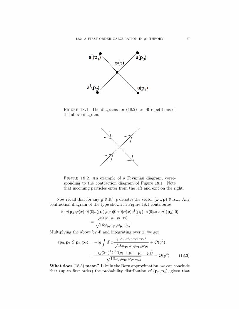
18.2. A FIRST-ORDER CALCULATION IN ϕ4 THEORY 77
Figure 18.1. The diagrams for (18.2) are 4! repetitions ofthe above diagram.
Figure 18.2. An example of a Feynman diagram, corre-sponding to the contraction diagram of Figure 18.1. Notethat incoming particles enter from the left and exit on the right.
Now recall that for any p ∈ R3, p denotes the vector (ωp,p) ∈ Xm. Anycontraction diagram of the type shown in Figure 18.1 contributes
〈0|a(p3)ϕ(x)|0〉〈0|a(p4)ϕ(x)|0〉〈0|ϕ(x)a†(p1)|0〉〈0|ϕ(x)a†(p2)|0〉
=ei(x,p3+p4−p1−p2)√16ωp1ωp2ωp3ωp4
.
Multiplying the above by 4! and integrating over x, we get
〈p3,p4|S|p1,p2〉 = −ig∫d4x
ei(x,p3+p4−p1−p2)√16ωp1ωp2ωp3ωp4
+O(g2)
=−ig(2π)4δ(4)(p3 + p4 − p1 − p2)√
16ωp1ωp2ωp3ωp4
+O(g2). (18.3)
What does (18.3) mean? Like in the Born approximation, we can concludethat (up to first order) the probability distribution of (p3,p4), given that

78 18. A FIRST-ORDER CALCULATION IN ϕ4 THEORY
the scattering has resulted in two outgoing particles, is supported on themanifold
(p3,p4) : p3 + p4 = p1 + p2Note that this is a manifold in R6 described by 4 constraints. Therefore weexpect this to be a 2D manifold. You can define a notion of ‘Lebesgue mea-sure’ on this manifold as the limit of a sequence of measures with densitiesproportional to
exp
(−‖p3 + p4 − p1 − p2‖2
ε
)as ε → 0, where the multiplicative factor is taken in such a way as to givea nontrivial limit. The scattering amplitude implies that the conditionalp.d.f. of (p3,p4) with respect to this ‘Lebesgue measure’ on the manifold isproportional to
1
ωp3ωp4
.
The constraint p03 + p0
4 = p01 + p0
2 shows that the manifold is bounded.Since the above density is also bounded, we can conclude that the densityis integrable on the manifold and gives a legitimate probability measure.
The above reasoning can be made completely rigorous by replacing theimproper incoming state |p1,p2〉 by a proper state which approximates it(for example, a Gaussian density), and then taking a sequence of approxi-mations converging to the improper state.
Note that if we are in the non-relativistic limit, where |p1| m and|p2| m, the constraint p0
3 + p04 = p0
1 + p02 approximately says
p23
2m+
p24
2m=
p21
2m+
p22
2m,
which is conservation of classical kinetic energy.
18.3. Words of caution
One should be aware of two things about the above calculation. Bothhave been mentioned before but are worth repeating here. First, the calcu-lation is not rigorous because we do not know how to rigorously define ϕ4
theory, or justify the Dyson expansion for this theory. However, if we ignorethese two (severe) problems, the rest of the calculation can be easily madefully rigorous.
The second thing to be aware of is that ϕ4 theory does not describe anyknown particle. It is purely a hypothetical theory that exhibits many of thecomplexities of quantum field theories that describe real particles, and istherefore useful for introducing various tools and techniques.
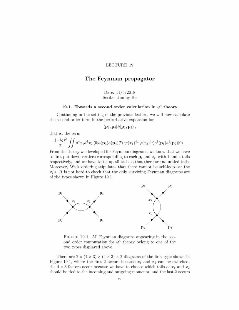
LECTURE 19
The Feynman propagator
Date: 11/5/2018Scribe: Jimmy He
19.1. Towards a second order calculation in ϕ4 theory
Continuing in the setting of the previous lecture, we will now calculatethe second order term in the perturbative expansion for
〈p3,p4|S|p1,p2〉 ,that is, the term
(−ig)2
2!
∫∫d4x1d
4x2 〈0|a(p3)a(p4)T (:ϕ(x1)4::ϕ(x2)4:)a†(p1)a†(p2)|0〉 .
From the theory we developed for Feynman diagrams, we know that we haveto first put down vertices corresponding to each pi and xi, with 1 and 4 tailsrespectively, and we have to tie up all tails so that there are no untied tails.Moreover, Wick ordering stipulates that there cannot be self-loops at thexi’s. It is not hard to check that the only surviving Feynman diagrams areof the types shown in Figure 19.1.
x1 x2
p1 p3
p2 p4
x1
x2
p3p1
p4p2
Figure 19.1. All Feynman diagrams appearing in the sec-ond order computation for ϕ4 theory belong to one of thetwo types displayed above.
There are 2 × (4 × 3) × (4 × 3) × 2 diagrams of the first type shown inFigure 19.1, where the first 2 occurs because x1 and x2 can be switched,the 4 × 3 factors occur because we have to choose which tails of x1 and x2
should be tied to the incoming and outgoing momenta, and the last 2 occurs
79

80 19. THE FEYNMAN PROPAGATOR
because we have decide how to tie the remaining tails of x1 and x2 to eachother. Similarly, there are 2× (4×3)× (4×3)×2×2 diagrams of the secondtype, where the extra factor of 2 comes from being able to switch p3 andp4. These are called one-loop diagrams because there is only one loop.
Let us analyze the first diagram. This corresponds to the followingproduct of contractions:
〈0|ϕ(x1)a†(p1)|0〉 〈0|ϕ(x1)a†(p2)|0〉· (〈0|T ϕ(x1)ϕ(x2))|0〉)2 〈0|a(p3)ϕ(x2))|0〉 〈0|a(p4)ϕ(x2))|0〉 .
We already know how to compute all but one of the terms in the aboveproduct, because we know that
〈0|a(p)ϕ(x)|0〉 =1√2ωp
ei(x,p),
〈0|ϕ(x)a†(p)|0〉 =1√2ωp
e−i(x,p).
(19.1)
We will now see how to compute 〈0|T ϕ(x1)ϕ(x2))|0〉.
19.2. The Feynman propagator
Definition 19.1. The Feynman propagator is a tempered distributionon R1,3 formally defined as
∆F (x) = i
∫d3p
(2π)32ωpe−i|t|ωp+ip·x (19.2)
where x = (t,x) and ωp =√
p2 +m2.
Note that ∆F (−x) = ∆F (x) because when we replace x by −x in theintegral, |t| is unchanged and p · x becomes −p · x, but we can do a changeof variable p 7→ −p to retrieve the original form.
Proposition 19.1. For any x1, x2 ∈ R1,3,
〈0|T ϕ(x1)ϕ(x2)|0〉 = −i∆F (x1 − x2).
Proof. Suppose that x1 = (t1,x1) and x2 = (t2,x2) with t1 ≥ t2. Then
〈0|T ϕ(x1)ϕ(x2)|0〉 = 〈0|ϕ(x1)ϕ(x2)|0〉 .Recall that ϕ(x) = A(fx)+A†(fx) where fx = ei(x,p). Thus by Lemma 17.1,
〈0|ϕ(x1)ϕ(x2)|0〉 = (fx1 , fx2) =
∫dλm(p)fx1(p)∗fx2(p)
=
∫dλm(p)ei(x2−x1,p)
=
∫d3p
(2π)3
1
2ωpei(x2−x1,p) = −i∆F (x1 − x2).
A similar derivation works if t1 < t2.
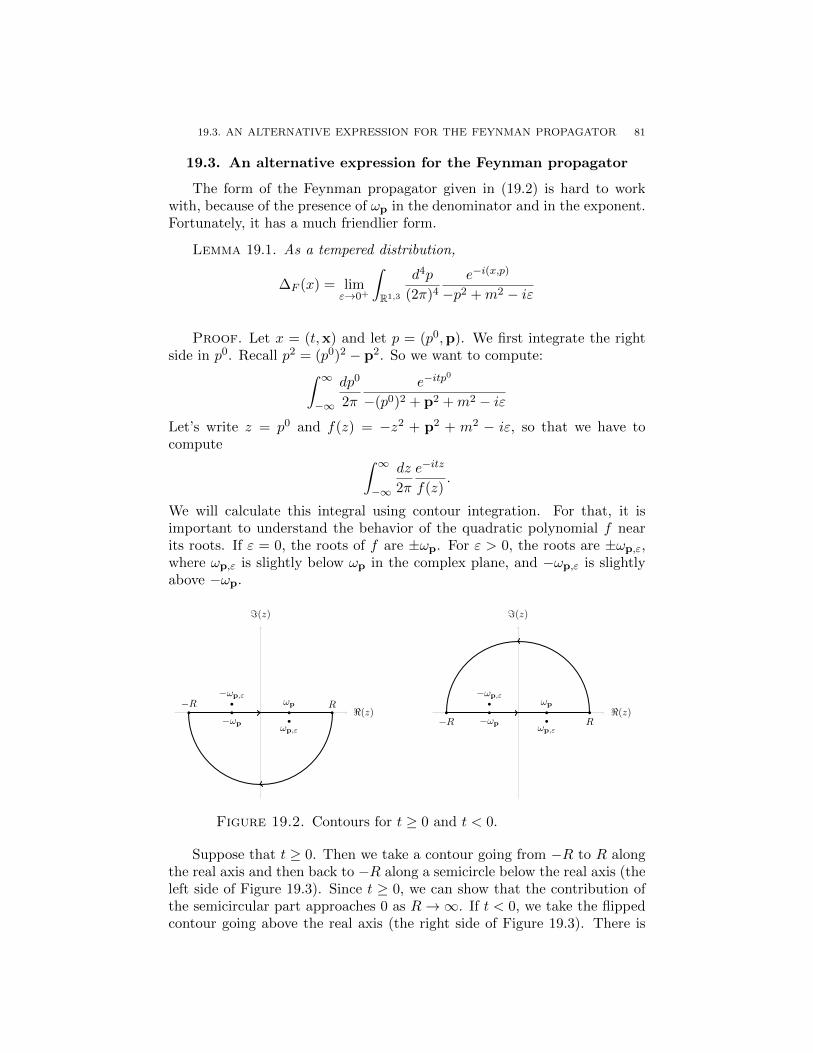
19.3. AN ALTERNATIVE EXPRESSION FOR THE FEYNMAN PROPAGATOR 81
19.3. An alternative expression for the Feynman propagator
The form of the Feynman propagator given in (19.2) is hard to workwith, because of the presence of ωp in the denominator and in the exponent.Fortunately, it has a much friendlier form.
Lemma 19.1. As a tempered distribution,
∆F (x) = limε→0+
∫R1,3
d4p
(2π)4
e−i(x,p)
−p2 +m2 − iε
Proof. Let x = (t,x) and let p = (p0,p). We first integrate the rightside in p0. Recall p2 = (p0)2 − p2. So we want to compute:∫ ∞
−∞
dp0
2π
e−itp0
−(p0)2 + p2 +m2 − iεLet’s write z = p0 and f(z) = −z2 + p2 + m2 − iε, so that we have tocompute ∫ ∞
−∞
dz
2π
e−itz
f(z).
We will calculate this integral using contour integration. For that, it isimportant to understand the behavior of the quadratic polynomial f nearits roots. If ε = 0, the roots of f are ±ωp. For ε > 0, the roots are ±ωp,ε,where ωp,ε is slightly below ωp in the complex plane, and −ωp,ε is slightlyabove −ωp.
ωp
ωp,ε−ωp
−ωp,ε
−R R <(z)
=(z)
ωp
ωp,ε−ωp
−ωp,ε
−R R<(z)
=(z)
Figure 19.2. Contours for t ≥ 0 and t < 0.
Suppose that t ≥ 0. Then we take a contour going from −R to R alongthe real axis and then back to −R along a semicircle below the real axis (theleft side of Figure 19.3). Since t ≥ 0, we can show that the contribution ofthe semicircular part approaches 0 as R→∞. If t < 0, we take the flippedcontour going above the real axis (the right side of Figure 19.3). There is
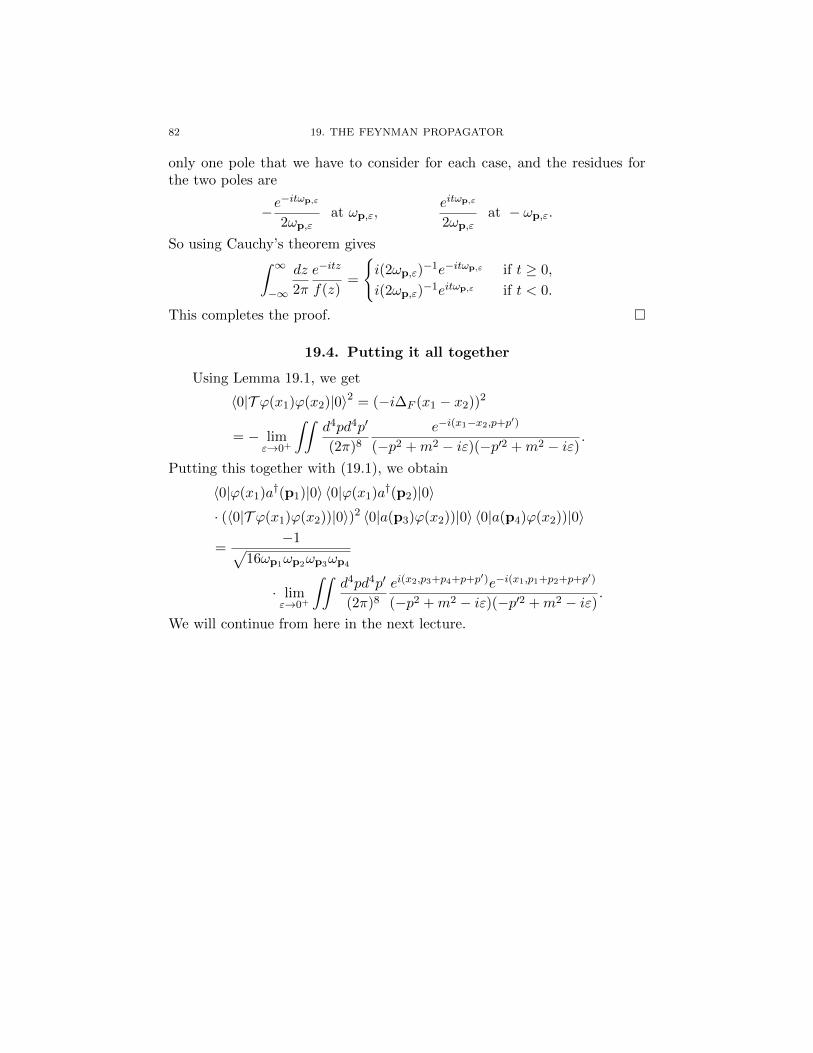
82 19. THE FEYNMAN PROPAGATOR
only one pole that we have to consider for each case, and the residues forthe two poles are
−e−itωp,ε
2ωp,εat ωp,ε,
eitωp,ε
2ωp,εat − ωp,ε.
So using Cauchy’s theorem gives∫ ∞−∞
dz
2π
e−itz
f(z)=
i(2ωp,ε)
−1e−itωp,ε if t ≥ 0,
i(2ωp,ε)−1eitωp,ε if t < 0.
This completes the proof.
19.4. Putting it all together
Using Lemma 19.1, we get
〈0|T ϕ(x1)ϕ(x2)|0〉2 = (−i∆F (x1 − x2))2
= − limε→0+
∫∫d4pd4p′
(2π)8
e−i(x1−x2,p+p′)
(−p2 +m2 − iε)(−p′2 +m2 − iε) .
Putting this together with (19.1), we obtain
〈0|ϕ(x1)a†(p1)|0〉 〈0|ϕ(x1)a†(p2)|0〉· (〈0|T ϕ(x1)ϕ(x2))|0〉)2 〈0|a(p3)ϕ(x2))|0〉 〈0|a(p4)ϕ(x2))|0〉
=−1√
16ωp1ωp2ωp3ωp4
· limε→0+
∫∫d4pd4p′
(2π)8
ei(x2,p3+p4+p+p′)e−i(x1,p1+p2+p+p′)
(−p2 +m2 − iε)(−p′2 +m2 − iε) .
We will continue from here in the next lecture.

LECTURE 20
The problem of infinities
Date: 11/7/2018Scribe: Sohom Bhattacharya
20.1. Completing the second order calculation in ϕ4 theory
Let us continue from where we stopped in the previous lecture. Recallthat we were trying to calculate the second order term in the perturbativeexpansion for a scattering amplitude in ϕ4 theory, and we ended up with aterm containing the integral
limε→0+
∫ ∫d4pd4p′
(2π)8
ei(x2,p3+p4+p+p′)e−i(x1,p1+p2+p+p′)
(−p2 +m2 − iε)(−(p′)2 +m2 − iε) .
To get the second order term in the Dyson series, we have to integrate thiswith respect to x1 and x2. Note that∫∫
d4x1d4x2e
i(x2,p3+p4+p+p′)−i(x1,p1+p2+p+p′)
= (2π)8δ(4)(p3 + p4 + p+ p′)δ(4)(p1 + p2 + p+ p′).
Recall the identity∫ ∞−∞
δ(x− z)δ(y − z)ξ(z)dz = δ(x− y)ξ(x),
which holds true in higher dimensions also. Using this identity, and ex-changing integrals and limits at will, we get
limε→0+
∫∫∫∫d4x1d
4x2
∫d4p
(2π)4
d4p′
(2π)4
ei(x2,p3+p4+p+p′)−i(x1,p1+p2+p+p′)
(−p2 +m2 − iε)(−p′2 +m2 − iε)
= limε→0+
∫∫d4pd4p′
δ(4)(p3 + p4 + p+ p′)δ(4)(p1 + p2 + p+ p′)
(−p2 +m2 − iε)(−p′2 +m2 − iε)
= limε→0+
∫d4p
δ(4)(p3 + p4 − p1 − p2)
(−p2 +m2 − iε)(−(−p1 − p2 − p)2 +m2 − iε) ,
which finally by a change of variable p 7→ −p yields
limε→0+
∫d4p
δ(4)(p3 + p4 − p1 − p2)
(−p2 +m2 − iε)(−(p1 + p2 − p)2 +m2 − iε) .
83

84 20. THE PROBLEM OF INFINITIES
Now let
M1 = limε→0+
∫d4p
(2π)4
1
(−p2 +m2 − iε)(−(p1 + p2 − p)2 +m2 − iε) ,
which is just the previous expression but without the Dirac delta, and di-vided by (2π)4. Recalling the discussion from the previous lecture and thefirst-order computation we did before, we now see that
〈p3,p4|S|p1,p2〉
= (g − ig2M +O(g3))−i(2π)4δ(4)(p3 + p4 − p1 − p2)√
16ωp1ωp2ωp3ωp4
, (20.1)
where M is the sum of several terms like M1, multiplied by some appropriatecombinatorial factor. (It is not hard to argue that the δ(4) and the ω’s wouldoccur in every term of the perturbative expansion just as they did in thefirst and second terms, which allows us to bring the O(g3) term inside thebracket.)
The big issue with the integral defining M1 is that the integrand decayslike ‖p‖−4 as ‖p‖ → ∞ and this makes the integral divergent. This is thesimplest instance of the ‘problem of infinities’ in quantum field theory.
20.2. The idea of renormalization
The quantity we are interested in is g − ig2M . The theory gives Mas a divergent integral. However, experiment gives M as a finite quantity(strictly speaking, not in ϕ4 theory, but in models that represent real phe-nomena). Therefore, obviously there is something wrong with the theory.The optimistic viewpoint is that the theory is approximately correct, whichmeans that the integral which diverged must be replaced with an integralwhich converges by multiplying the integrand by a cutoff function, which isgiven by nature but unknown to us. For example, in our context, this meansthat M should be replaced by something like
M = limε→0+
∫d4p
(2π)4
θ(p)
(−p2 +m2 − iε)(−(p1 + p2 − p)2 +m2 − iε)+ other similar terms,
where θ(p) is a function that always takes values between 0 and 1, satisfiesθ(p) = 1 when |p| ≤ R for some large R, and decays fast enough in theregion |p| > R so that the integral converges. Further, we assume that g
is so small that we can effectively treat M as a large but fixed value whileworking out the perturbative expansion in g. Thus, terms like O(gk) may
implicitly contain powers of quantities like M .The problem is that we do not know the cutoff function θ that is provided
by nature. This hurdle is overcome as follows, which is the main idea in
renormalization. Suppose that we can observe the value of M for certainvalues p∗1, p∗2, p∗3, p∗4 of the incoming and outgoing momenta. For example,

20.2. THE IDEA OF RENORMALIZATION 85
they may all be close to (m, 0, 0, 0), which is the non-relativistic scenario
realized in a laboratory experiment. Call this value M∗. Then the theory
will allow you to calculate M for any p1, p2, p3, p4, even if you do notknow the cutoff function or the coupling constant, through a process calledrenormalization. This is roughly described as follows, for the problem thatwe are discussing.
For the laboratory values p∗1, p∗2, p∗3, p∗4, suppose that the true observedamplitude is
A∗−i(2π)4δ(4)(p∗3 + p∗4 − p∗1 − p∗2)√
16ωp∗1ωp∗2
ωp∗3ωp∗4
.
(Here we assume that p∗3 + p∗4 − p∗1 − p∗2 = 0, so that A∗ can be measured.)Then by (20.1),
A∗ = g − ig2M∗ +O(g3), (20.2)
where M∗ is the value of M in the laboratory setting. Also, for our givenp1, p2, p3, p4,
〈p3,p4|S|p1,p2〉 = A−i(2π)4δ(4)(p3 + p4 − p1 − p2)√
16ωp1ωp2ωp3ωp4
,
where
A = g − ig2M +O(g3). (20.3)
The quantity A is our main object of interest, which we cannot evaluate ifwe do not know the cutoff function θ. We will now argue that in fact we canapproximately evaluate A even if do not know θ, purely using the amplitudeA∗ observed in the laboratory. To see this, first note that by (20.2),
g = A∗ + ig2M∗ +O(g3). (20.4)
Next, note that since A∗ = O(g), squaring the equation (20.2) we obtain
g2 = A2∗ +O(g3). (20.5)
Substituting the values of g and g2 from (20.4) and (20.5) into (20.3), weget
A = A∗ + ig2M∗ − ig2M +O(g3)
= A∗ − iA2∗(M − M∗) +O(g3). (20.6)
It turns out that if the cutoff function θ satisfies θ(p) ∈ [0, 1] for all p,θ(p) = 1 for |p| ≤ R, and decays fast enough the region |p| > R, then thelimit
L := limR→∞
(M − M∗)exists and is finite, irrespective of how θ varies with R, as long as it satisfiesthe above constraints. (We will prove this in the next couple of lectures.)
We can then substitute L for M −M∗ in (20.6) to get an approximate valueof A in terms of A∗, with O(g3) error. This is the key idea in perturbative

86 20. THE PROBLEM OF INFINITIES
renormalization, which becomes harder to manage for higher orders of per-turbation theory. If, however, it can be done for all orders, the theory iscalled ‘perturbatively renormalizable’.
Note that the above calculation was slightly complicated because wewanted to get an approximation for A solely in terms of A∗, and not usingany information about θ or g. If we know g, then the problem becomes
easier, because we can simply approximate M by L+ M∗ in (20.3).

LECTURE 21
One-loop renormalization in ϕ4 theory
Date: 11/9/2018Scribe: Laura Lyman
21.1. A toy example
Recall the basic idea of renormalization from the previous lecture: Sup-pose that we want to carry out a calculation for a physical system, where weinput some quantity a, where a can be a vector or scalar (e.g. the 4-tuple ofincoming and outgoing momenta p1, p2, p3, p4, as considered in the previ-ous lecture), and the output is a scalar f(a) (e.g. the probability amplitude〈p3,p4|S|p1,p2〉). As seen in the previous lecture, sometimes the theorywill yield a prediction for f(a) in terms of divergent integrals. However theobserved value of f(a) is finite. The optimistic viewpoint is that the theoryis approximately correct, in the sense that the divergent integrals shouldbe replaced with integrals with some cutoffs (regularized versions). Natureprovides the cutoff function θ, but it is unknown to us. The solution to thisobstacle is that we can still approximately recover f(a) if we know f(a′) forany single a′ even if θ is unknown. When this can be done for all orders ofperturbation theory, the theory is called perturbatively renormalizable.
To understand the situation, consider the following toy example. Sup-pose that the input quantity is some number a > 0, and the output predictedby theory is
ftheory(a) =
∫ ∞0
dx
x+ a=∞.
However, suppose that the experimentally observed output f(a) is alwaysfinite. To resolve this discrepancy, assume that the theory is approximatelycorrect, in the sense that the true f(a) is given by
f(a) =
∫ ∞0
θ(x)dx
x+ a
where θ is a function such that θ(x) ∈ [0, 1] for all x, θ(x) = 1 when x ≤ Rfor some large R ∈ R, and θ decays sufficiently fast in the region x > R sothat the integral converges. Then
f(a)− f(a′) =
∫ ∞0
θ(x)(a′ − a)dx
(x+ a)(x+ a′)=
∫ ∞0
dx(a− a′)(x+ a)(x+ a′)
+O(1/R).
87

88 21. ONE-LOOP RENORMALIZATION IN ϕ4 THEORY
Thus, we can approximately recover f(a) for any a if we observe the valueof f(a′) for some a′, even if we do not know θ.
21.2. Main result
Recall that we were trying to calculate the second order term in theDyson expansion of
〈p3,p4|S|p1,p2〉.There were no divergent integrals in the first order term. However, in thesecond order, each Feynman diagram had a single loop, which gave divergentintegrals like
limε→0+
∫d4p
(2π)4
1
(−p2 +m2 − iε)(−(w − p)2 +m2 − iε)where w = p1 + p2. Let us therefore assume that the “true” value is
U(w, θ) := limε→0+
∫d4p
(2π)4
θ(p)
(−p2 +m2 − iε)(−(w − p)2 +m2 − iε)where θ : R3 → [0, 1] is a function such that θ(p) = 1 when |p| ≤ R, and θdecays sufficiently fast in the region |p| > R. The following theorem showsthat the above integral can be approximately computed for any w if we knowits value at a single w′, even if we do not know θ.
Theorem 21.1 (One-loop renormalization). For any w,w′ ∈ R1,3
limR→∞
(U(w, θ)− U(w′, θ))
exists, is finite, and depends only on (w,w′). Here we assume that θ varieswith R in such a way that we always have θ(p) = 1 for |p| ≤ R.
Why is the situation of Theorem 21.1 harder to analyze than the toyexample discussed above? The difference is that terms like −p2 +m2 in thedenominator introduce infinite manifolds of singularities as ε → 0. To getrid of such singularities, we need two technical tools.
Lemma 21.1 (Feynman parameter). Suppose that A,B ∈ C are suchthat the line segment joining A and B in the complex plane does not passthrough 0. Then
1
AB=
∫ 1
0du
1
(Au+B(1− u))2.
(Here u is called a Feynman parameter.)
Proof. Note that
d
du
[1
(B −A)(Au+B(1− u))
]=
1
(Au+B(1− u))2,
and substitute above.

21.2. MAIN RESULT 89
Lemma 21.2 (Wick rotation). Suppose that f : C→ C is a holomorphicfunction which has no poles in the region x + iy : xy ≥ 0. Furthermore,suppose that |f(z)| ≤ C|z|−1−ε in this region for some C < ∞ and ε > 0.Then ∫ ∞
−∞dxf(x) = i
∫ ∞−∞
dxf(ix).
Proof. To see this, consider the following contour. Starting from theorigin, traverse the blue path and then the red path in Figure 21.1.
R
−R
iR
0
−iR
Figure 21.1. Contour traversed from the origin first alongthe blue path and then along the red path.
Note that f has no poles enclosed by this contour. The decay conditionimplies that the integral contribution on the circular arcs tends to 0 as R→∞. Thus, the result follows by Cauchy’s theorem and taking R→∞.
Corollary 21.1. For any α > 0, E ∈ R, and ε > 0,∫ ∞−∞
dx1
(−αx2 + E − iε)2= i
∫ ∞−∞
dx1
(αx2 + E − iε)2.
Proof. Since ε > 0, it is easy to see that the integrals are both well-defined and finite. Let
f(z) =1
(−αz2 + E − iε)2.
Then there is some constant C such that |f(z)| ≤ C|z|−2 for all |z|. More-over, observe that
−αz2 = −α(x2 − y2 + 2ixy) = −α(x2 − y2)− 2iαxy.
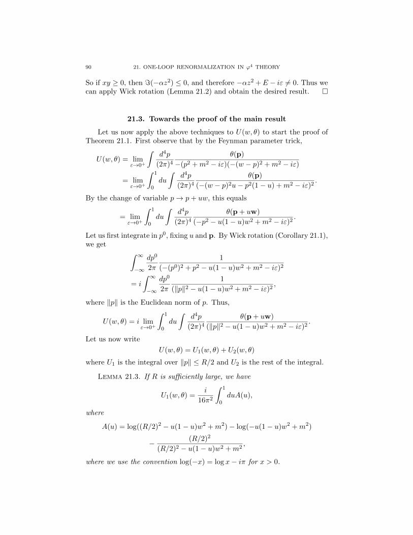
90 21. ONE-LOOP RENORMALIZATION IN ϕ4 THEORY
So if xy ≥ 0, then =(−αz2) ≤ 0, and therefore −αz2 +E − iε 6= 0. Thus wecan apply Wick rotation (Lemma 21.2) and obtain the desired result.
21.3. Towards the proof of the main result
Let us now apply the above techniques to U(w, θ) to start the proof ofTheorem 21.1. First observe that by the Feynman parameter trick,
U(w, θ) = limε→0+
∫d4p
(2π)4
θ(p)
−(p2 +m2 − iε)(−(w − p)2 +m2 − iε)
= limε→0+
∫ 1
0du
∫d4p
(2π)4
θ(p)
(−(w − p)2u− p2(1− u) +m2 − iε)2.
By the change of variable p→ p+ uw, this equals
= limε→0+
∫ 1
0du
∫d4p
(2π)4
θ(p + uw)
(−p2 − u(1− u)w2 +m2 − iε)2.
Let us first integrate in p0, fixing u and p. By Wick rotation (Corollary 21.1),we get ∫ ∞
−∞
dp0
2π
1
(−(p0)2 + p2 − u(1− u)w2 +m2 − iε)2
= i
∫ ∞−∞
dp0
2π
1
(‖p‖2 − u(1− u)w2 +m2 − iε)2,
where ‖p‖ is the Euclidean norm of p. Thus,
U(w, θ) = i limε→0+
∫ 1
0du
∫d4p
(2π)4
θ(p + uw)
(‖p‖2 − u(1− u)w2 +m2 − iε)2.
Let us now write
U(w, θ) = U1(w, θ) + U2(w, θ)
where U1 is the integral over ‖p‖ ≤ R/2 and U2 is the rest of the integral.
Lemma 21.3. If R is sufficiently large, we have
U1(w, θ) =i
16π2
∫ 1
0duA(u),
where
A(u) = log((R/2)2 − u(1− u)w2 +m2)− log(−u(1− u)w2 +m2)
− (R/2)2
(R/2)2 − u(1− u)w2 +m2,
where we use the convention log(−x) = log x− iπ for x > 0.
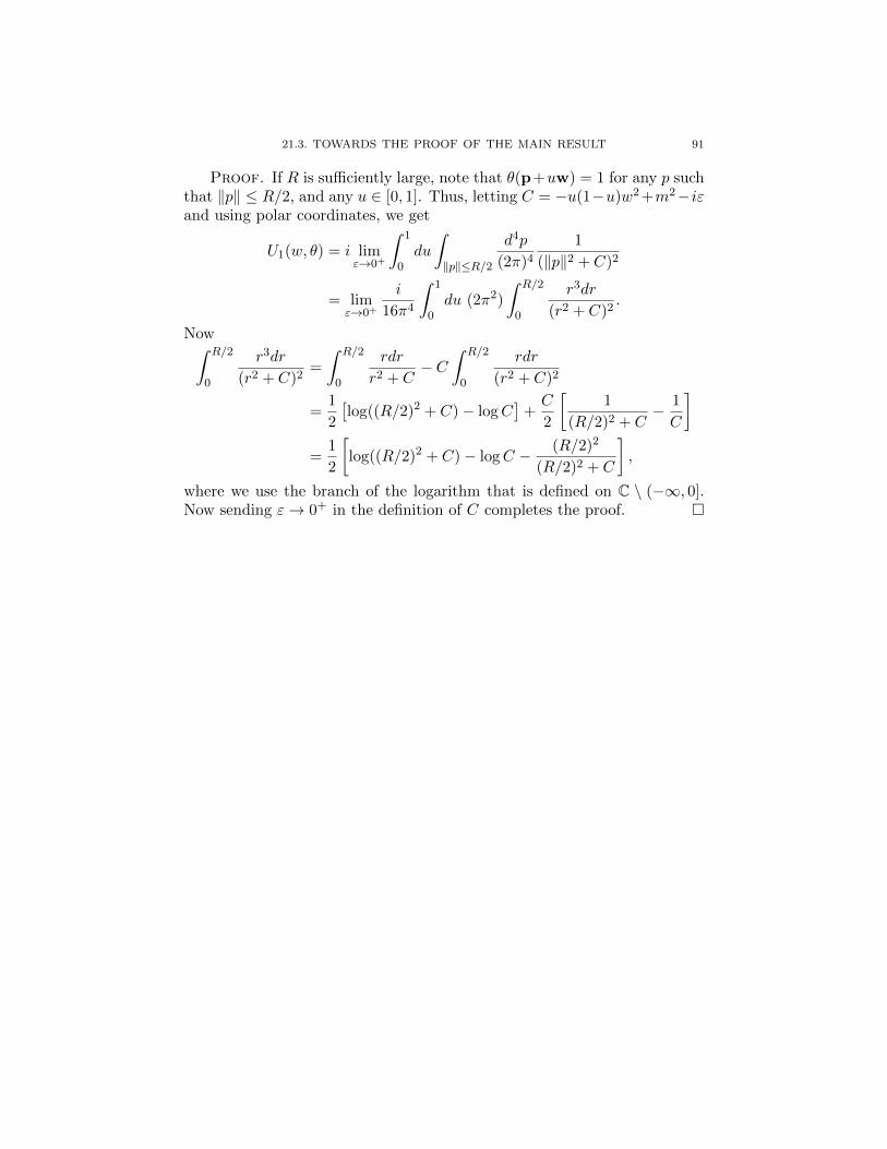
21.3. TOWARDS THE PROOF OF THE MAIN RESULT 91
Proof. If R is sufficiently large, note that θ(p+uw) = 1 for any p suchthat ‖p‖ ≤ R/2, and any u ∈ [0, 1]. Thus, letting C = −u(1−u)w2 +m2−iεand using polar coordinates, we get
U1(w, θ) = i limε→0+
∫ 1
0du
∫‖p‖≤R/2
d4p
(2π)4
1
(‖p‖2 + C)2
= limε→0+
i
16π4
∫ 1
0du (2π2)
∫ R/2
0
r3dr
(r2 + C)2.
Now∫ R/2
0
r3dr
(r2 + C)2=
∫ R/2
0
rdr
r2 + C− C
∫ R/2
0
rdr
(r2 + C)2
=1
2
[log((R/2)2 + C)− logC
]+C
2
[1
(R/2)2 + C− 1
C
]=
1
2
[log((R/2)2 + C)− logC − (R/2)2
(R/2)2 + C
],
where we use the branch of the logarithm that is defined on C \ (−∞, 0].Now sending ε→ 0+ in the definition of C completes the proof.


LECTURE 22
A glimpse at two-loop renormalization
Date: 11/12/2018Scribe: Lingxiao Li
22.1. Finishing the proof for one-loop renormalization
In this lecture we will first complete the proof of Theorem 21.1. Recallthe quantity U(w, θ) from the previous lecture and the decomposition U =U1 +U2. From the expression we obtained for U1(w, θ), it is easy to see that
limR→∞
(U1(w, θ)− U1(w′, θ)) = L(w)− L(w′),
where
L(w) =−i
16π2
∫ 1
0du log(m2 − u(1− u)w2).
As before, here we use the convention that log(−x) = log x− iπ when x > 0.Our next step is to prove the following lemma.
Lemma 22.1.
limR→∞
(U2(w, θ)− U2(w′, θ)) = 0.
This will imply Theorem 21.1, and will moreover prove that
limR→∞
(U(w, θ)− U(w′, θ)) = L(w)− L(w′).
Proof of Lemma 22.1. By definition, we have
U2(w, θ) = i limε→0+
∫ 1
0du
∫‖p‖≥R/2
d4p
(2π)4
θ(p + uw)
(‖p‖2 − u(1− u)w2 +m2 − iε)2.
If ‖p‖ is sufficiently large (by letting R be large), the denominator in theintegrand will be far away from 0, so we can interchange limit and integralsand send ε→ 0 to get
U2(w, θ) = i
∫ 1
0du
∫‖p‖≥R/2
d4p
(2π)4
θ(p + uw)
(‖p‖2 − u(1− u)w2 +m2)2
= i
∫ 1
0du
∫‖p−uw‖≥R/2
d4p
(2π)4
θ(p)
(‖p− uw‖2 − u(1− u)w2 +m2)2,
93

94 22. A GLIMPSE AT TWO-LOOP RENORMALIZATION
where the last step follows by the change of variable p 7→ p − uw. Let usfurther split the integral as
U3(w, θ) = i
∫ 1
0du
∫‖p‖≥R/2
d4p
(2π)4
θ(p)
(‖p− uw‖2 − u(1− u)w2 +m2)2,
and U4(w, θ) = U2(w, θ)−U3(w, θ). Let ∆(w,R) be the symmetric differenceof the regions p : ‖p‖ ≥ R/2 and p : ‖p − uw‖ ≥ R/2. Since θ ∈ [0, 1]everywhere, it follows that
|U4(w, θ)| ≤∫ 1
0du
∫∆(w,R)
d4p
(2π)4
1
(‖p− uw‖2 − u(1− u)w2 +m2)2.
Since Vol(∆(w,R)) = O(R3) and the integrand in the above display is oforder R−4 in ∆(w,R), it follows that |U4(w, θ)| = O(R−1) as R → ∞. Soto complete the proof of the lemma, it remains to show that
limR→∞
(U4(w, θ)− U4(w′, θ)) = 0.
To prove this, note that
|U4(w, θ)− U4(w′, θ)| ≤∫ 1
0du
∫‖p‖≥R/2
d4p
(2π)4|θ(p)F (p, u, w,w′)|
≤∫ 1
0du
∫‖p‖≥R/2
d4p
(2π)4|F (p, u, w,w′)|,
where
F (p, u, w,w′) =1
(‖p‖2 − u(1− u)w2 +m2)2
− 1
(‖p‖2 − u(1− u)w′2 +m2)2.
It is easy to see that there is some R0 and some C, depending only on m,w and w′, such that |F (p, u, w,w′)| ≤ C‖p‖−5 whenever ‖p‖ ≥ R0. Thus,
limR→∞
|U4(w, θ)− U4(w′, θ)| ≤ limR→∞
∫ 1
0du
∫‖p‖≥R/2
d4p
(2π)4C‖p‖−5 = 0.
This completes the proof of the lemma and hence of Theorem 21.1.
22.2. Wick ordering as a form of renormalization
Suppose we use ϕ(x)4 in the Hamiltonian of ϕ4 theory instead of :ϕ(x)4:.Then we will end up getting many more exploding integrals, like the oneshere, even in the first order of perturbation theory. But after renormaliza-tion, all these infinities will cancel out, and we will get exactly the samepredictions as we did in the Wick ordered version. Hence Wick ordering islike a ‘preemptive’ renormalization.
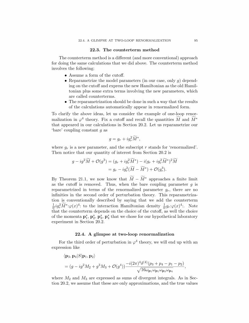
22.4. A GLIMPSE AT TWO-LOOP RENORMALIZATION 95
22.3. The counterterm method
The counterterm method is a different (and more conventional) approachfor doing the same calculations that we did above. The counterterm methodinvolves the following:
• Assume a form of the cutoff.• Reparametrize the model parameters (in our case, only g) depend-
ing on the cutoff and express the new Hamiltonian as the old Hamil-tonian plus some extra terms involving the new parameters, whichare called counterterms.• The reparametrization should be done in such a way that the results
of the calculations automatically appear in renormalized form.
To clarify the above ideas, let us consider the example of one-loop renor-
malization in ϕ4 theory. Fix a cutoff and recall the quantities M and M∗
that appeared in our calculations in Section 20.2. Let us reparametrize our‘bare’ coupling constant g as
g = gr + ig2rM∗,
where gr is a new parameter, and the subscript r stands for ‘renormalized’.Then notice that our quantity of interest from Section 20.2 is
g − ig2M +O(g3) = (gr + ig2rM∗)− i(gr + ig2
rM∗)2M
= gr − ig2r (M − M∗) +O(g3
r ).
By Theorem 21.1, we now know that M − M∗ approaches a finite limitas the cutoff is removed. Thus, when the bare coupling parameter g isreparametrized in terms of the renormalized parameter gr, there are noinfinities in the second order of perturbation theory. This reparametriza-tion is conventionally described by saying that we add the counterterm14! ig
2rM∗:ϕ(x)4: to the interaction Hamiltonian density 1
4!gr:ϕ(x)4:. Notethat the counterterm depends on the choice of the cutoff, as well the choiceof the momenta p∗1, p∗2, p∗3, p∗4 that we chose for our hypothetical laboratoryexperiment in Section 20.2.
22.4. A glimpse at two-loop renormalization
For the third order of perturbation in ϕ4 theory, we will end up with anexpression like
〈p3,p4|S|p1,p2〉
= (g − ig2M2 + g3M3 +O(g4))−i(2π)4δ(4)(p3 + p4 − p1 − p2)√
16ωp1ωp1ωp3ωp4
,
where M2 and M3 are expressed as sums of divergent integrals. As in Sec-tion 20.2, we assume that these are only approximations, and the true values
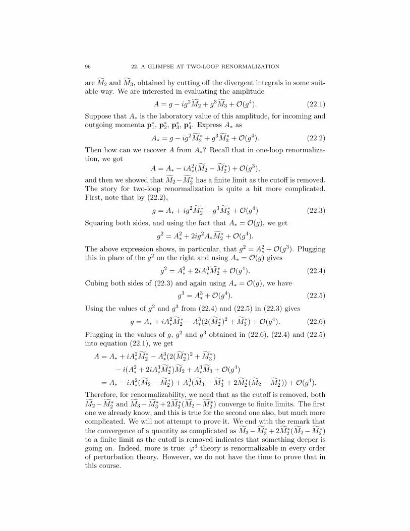
96 22. A GLIMPSE AT TWO-LOOP RENORMALIZATION
are M2 and M3, obtained by cutting off the divergent integrals in some suit-able way. We are interested in evaluating the amplitude
A = g − ig2M2 + g3M3 +O(g4). (22.1)
Suppose that A∗ is the laboratory value of this amplitude, for incoming andoutgoing momenta p∗1, p∗2, p∗3, p∗4. Express A∗ as
A∗ = g − ig2M∗2 + g3M∗3 +O(g4). (22.2)
Then how can we recover A from A∗? Recall that in one-loop renormaliza-tion, we got
A = A∗ − iA2∗(M2 − M∗2 ) +O(g3),
and then we showed that M2−M∗2 has a finite limit as the cutoff is removed.The story for two-loop renormalization is quite a bit more complicated.First, note that by (22.2),
g = A∗ + ig2M∗2 − g3M∗3 +O(g4) (22.3)
Squaring both sides, and using the fact that A∗ = O(g), we get
g2 = A2∗ + 2ig2A∗M
∗2 +O(g4).
The above expression shows, in particular, that g2 = A2∗ +O(g3). Plugging
this in place of the g2 on the right and using A∗ = O(g) gives
g2 = A2∗ + 2iA3
∗M∗2 +O(g4). (22.4)
Cubing both sides of (22.3) and again using A∗ = O(g), we have
g3 = A3∗ +O(g4). (22.5)
Using the values of g2 and g3 from (22.4) and (22.5) in (22.3) gives
g = A∗ + iA2∗M∗2 −A3
∗(2(M∗2 )2 + M∗3 ) +O(g4). (22.6)
Plugging in the values of g, g2 and g3 obtained in (22.6), (22.4) and (22.5)into equation (22.1), we get
A = A∗ + iA2∗M∗2 −A3
∗(2(M∗2 )2 + M∗3 )
− i(A2∗ + 2iA3
∗M∗2 )M2 +A3
∗M3 +O(g4)
= A∗ − iA2∗(M2 − M∗2 ) +A3
∗(M3 − M∗3 + 2M∗2 (M2 − M∗2 )) +O(g4).
Therefore, for renormalizability, we need that as the cutoff is removed, both
M2−M∗2 and M3−M∗3 +2M∗2 (M2−M∗2 ) converge to finite limits. The firstone we already know, and this is true for the second one also, but much morecomplicated. We will not attempt to prove it. We end with the remark that
the convergence of a quantity as complicated as M3− M∗3 + 2M∗2 (M2− M∗2 )to a finite limit as the cutoff is removed indicates that something deeper isgoing on. Indeed, more is true: ϕ4 theory is renormalizable in every orderof perturbation theory. However, we do not have the time to prove that inthis course.

22.5. COUNTERTERMS FOR TWO-LOOP RENORMALIZATION 97
22.5. Counterterms for two-loop renormalization
Instead of the relatively complicated derivation above, we could havealso used the counterterm method for two-loop renormalization in ϕ4 the-ory. The proper way to use the counterterm method for this purpose is toreparametrize g as
g = gr + ig2rM∗2 − g3
r (M∗3 + 2(M∗2 )2).
Indeed, an easy verification shows that plugging the above into (22.1) gives
A = gr − ig2r (M2 − M∗2 ) + g3
r (M3 − M∗3 + 2M∗2 (M2 − M∗2 )) +O(g4r ).
Thus, if we accept out previous claim that M3 − M∗3 + 2M∗2 (M2 − M∗2 )converges to a finite limit as the cutoff is removed, then there are no infinitiesin the third order of perturbation theory for ϕ4 theory after adding the
counterterms 14! ig
2rM∗2 :ϕ(x)4: and − 1
4!g3r (M3−M∗3 +2M∗2 (M2−M∗2 )):ϕ(x)4:
to the the interaction Hamiltonian density 14!gr:ϕ(x)4:.

LECTURE 23
The model for free photons
Date: 11/14/2018Scribe: Alex Dunlap
23.1. Photons
Photons are massless particles moving at the speed of light. In thislecture we will construct a model for free photons. This is a real model thatis used in physics.
Recall that the four-momentum of a particle with mass m and velocityv (in some coordinate system) is the vector
p =
(m√
1− v2,
mv√1− v2
). (23.1)
For photons, m = 0 and |v| = 1, so we get 0/0 in (23.1). However, we alsoknow that the four-momentum of a particle of mass m satisfies p2 = m2, sothat p ∈ Xm. There is no problem in defining the manifold
X0 = p : p2 = 0, p0 ≥ 0.(This is just the surface of a cone in R1,3.) So we can hypothesize thatphotons also have four-momenta, which belong to X0. The manifold X0
comes equipped with the Lorentz-invariant measure λ0, defined as before.We will later use the fact that λ0 has no point masses.
It is a physical fact the four-momentum is not the only quantity thatcharacterizes a photon. A photon also has some internal degrees of freedom,called spin. Therefore it does not suffice to take L2(X0, dλ0) to be theHilbert space for photons. Constructing the Hilbert space for photons is aslightly complicated affair, which we now carry out.
23.2. The Gupta–Bleuler construction
The procedure for constructing the Hilbert space for photons is calledthe Gupta–Bleuler quantization. It goes as follows. Start with the vectorspace of all f : X0 → C4 such that each coordinate of f is in L2(X0, dλ0),which is denoted by L2(X0, dλ0,C4). We will simply call this space H. (Thisis not the final Hilbert space, but we’ll use it.) For w, z ∈ C4, define theMinkowski inner product
(w, z) = (w0)∗z0 − (w1)∗z1 − (w2)∗z2 − (w3)∗z3.
99
100 23. THE MODEL FOR FREE PHOTONS
If Λ ∈ SO↑(1, 3), define Λz as expected: if z ∈ C4 equals x+ iy, with x, y ∈R4, then let Λz = Λx + iΛy. It is simple to check that (Λz,Λw) = (z, w).For ξ, ψ ∈ H, define
(ξ, ψ) = −∫dλ0(p) (ξ(p), ψ(p)). (23.2)
This defines a sesquilinear form on H, but it is not positive-definite. Toextract a subspace on which this form is positive semidefinite, define
H′ = ξ ∈ H : (p, ξ(p)) = 0 for λ0-a.e. p.
Lemma 23.1. The inner product defined in (23.2) is positive semidefiniteon H′.
Proof. Take any ξ ∈ H′. Suppose that p is a point so that (p, ξ(p)) = 0,and p 6= 0. Write
p = (p0,p) = (p0, p1, p2, p3).
Since p ∈ X0, we have
(p0)2 = (p1)2 + (p2)2 + (p3)2.
Also, p 6= 0. So p0 > 0 and p 6= 0. Let A ∈ SO(3) be such that Ap = (0, 0, a)for some a. Since A is a rotation, |a| = |p|. Moreover, we can arrange it sothat a = |p| = p0. Let
Λ =
(1 00 A
)∈ SO↑(1, 3).
Let x = ξ(p), and let z = Λx. Note that Λp = (p0, 0, 0, p0). Thus,
(p, x) = (Λp,Λx) = (Λp, z) = p0(z0 − z3).
But we know that
(p, x) = (p, ξ(p)) = 0,
and p0 > 0. Therefore, z0 = z3. Then
(ξ(p), ξ(p)) = (z, z) = (z0)2 − (z1)2 − (z2)2 − (z3)2 = −(z1)2 − (z2)2 ≤ 0.
Therefore, (ξ, ξ) ≥ 0, using that λ0 has no point mass at 0. This completesthe proof of the lemma.
Having defined H′, define Hnull = ξ ∈ H′ : (ξ, ξ) = 0. Define Hphys =H′/Hnull. ThenHphys is a Hilbert space under the Minkowski inner product.One can also check that it is complete. This is the Hilbert space for a singlephoton. For arbitrary numbers of photons, we take the bosonic Fock spaceof Hphys.

23.3. THE REPRESENTATION FOR A FREE PHOTON 101
23.3. The representation for a free photon
Having defined the Hilbert space, it remains to define the representationof the Poincare group that describes the spacetime trajectory of a photon.Recall that in quantum field theory, the full spacetime description of a sys-tem is given by a state in a Hilbert space. Recall also the definition of thePoincare group P = R1,3 o SO↑(1, 3), which is the group of symmetries ofR1,3. The action is of (a,A) ∈ P on a point x ∈ R1,3 is (a,A)x = a + Ax.Finally, recall the postulate that for any quantum system, there is a stronglycontinuous unitary representation U of P in the Hilbert space for the sys-tem, such that if an observer sees the system in state ψ, then in the differentcoordinate system obtained by the action of (a,A), the system appears tobe in state U(a,A)ψ.
The representation U of P in Hphys that describes the evolution of a freephoton is defined as follows. For ψ ∈ H, define
(U(a,A)ψ)(p) = ei(a,p)Aψ(A−1p).
It is easy to check that this is a representation of P in H. Moreover, it iseasy to check that U(a,A) maps H′ into H′, and moreover it descends toa representation in Hphys. To prove the first claim, note that since λ0 isLorentz-invariant and (p, ψ(p)) = 0 for λ0-a.e. p for any ψ ∈ H′,∫
dλ0(p) (p, U(a,A)ψ(p)) =
∫dλ0(p) (p, ei(a,p)Aψ(A−1p))
=
∫dλ0(p) ei(a,p) (A−1p, ψ(A−1p))︸ ︷︷ ︸
= 0 for λ0-a.e. p
= 0.
The proof of the second claim follows by showing that U(a,A) maps Hnullinto Hnull in a similar manner. Thus, U is a representation of P in Hphys.Moreover, U is a unitary representation:
(U(a,A)ψ,U(a,A)ξ) = −∫dλ0(p) (ei(a,p)Aψ(A−1p), ei(a,p)Aξ(A−1p))
= −∫dλ0(p) (Aψ(A−1p), Aξ(A−1p))
= −∫dλ0(p) (ψ(A−1p), ξ(A−1p))
= −∫dλ0(p) (ψ(p), ξ(p))
= (ψ, ξ),
where in the third equality, we used the fact that the inner product isLorentz-invariant, and in the fourth inequality, we used the fact that λ0
is Lorentz-invariant.
102 23. THE MODEL FOR FREE PHOTONS
23.4. The quantized electromagnetic four-potential
Just as we had the massive free field associated with our massive scalarboson, there is a field associated with photons. It’s called the electromag-netic four-potential. Consider our original H = L2(X0, dλ0,C4) with theEuclidean inner product, defined as
(ξ, ψ)E :=
∫dλ0(p)
3∑µ=0
ξµ(p)∗ψµ(p).
Then H is a Hilbert space under this inner product. Consider the Fock spaceB of this Hilbert space, and our familiar operator-valued distributions A andA†. Define two other operators B and B† as follows. Recall the matrix ηdefined in (9.1). Then for any ξ = (ξ0, ξ1, ξ2, ξ3) ∈ H, we can naturallydefine ηξ = (ξ0,−ξ1,−ξ2,−ξ3). Let
B(ξ) = A(−ηξ),B†(ξ) = A†(ξ).
Then B, B† are also operator-valued distributions on H, and they have theproperties that
[B(ξ), B(ψ)] = [B†(ξ), B†(ψ)] = 0,
[B(ξ), B†(ψ)] = (ξ, ψ)︸ ︷︷ ︸our inner product
1.
This is because
[B(ξ), B†(ψ)] = [A(−ηξ), A†(ψ)] = (−ηξ, ψ)E1 = (ξ, ψ)1.
For f ∈ S (R4), µ = 0, 1, 2, 3, define
Aµ(f) = B(f eµ) +B†(f eµ),
where eµ is the µth standard basis vector and f is the Fourier transformof f on R1,3, restricted to X0. The 4-tuple A = (A0, A1, A2, A3) is calledthe quantized electromagnetic four-potential. Each Aµ is an operator-valueddistribution that takes f ∈ S (R4) to a linear operator Aµ(f) on B0, whereB0 is our familiar dense subspace of the Fock space B.

LECTURE 24
The electromagnetic field
Date: 11/26/2018Scribe: Jae Hee Lee
24.1. Relationship between the two Hilbert spaces
Recall the spaces H, H′ and Hphys from the previous lecture. The spaceHphys is the Hilbert space for photons, whereas the quantized electromag-netic four-potential A was defined on H. Recall that H carries the Eu-clidean inner product, while the inner product on Hphys is derived from theMinkowski inner product on H′. So how are the two Hilbert spaces related?More importantly, how does the electromagnetic four-potential act on thebosonic Fock space for photons? This happens as follows.
Let B be the bosonic Fock space of H and let B′ be the bosonic Fockspace of H′ (all under the Euclidean inner product). Then B′ is a closedsubspace of B. The Minkowski sesquilinear form and the Minkowski normon H′ extends to B′ in the following way. We first define on the simpletensors
(ξ1 ⊗ · · · ⊗ ξn, ψ1 ⊗ · · · ⊗ ξn) =
n∏i=1
(ξi, ψi),
and use linearity and the inequality
‖ξ‖ =√
(ξ, ξ) ≤ ‖ξ‖E for ξ ∈ H′
to extend this to B′. Note that the expression√
(ξ, ξ) makes sense becausethe Minkowski form is nonnegative on H′. Next, we define
Bnull := ψ ∈ B′ : ‖ψ‖ = 0,which is a closed subspace of B′, and correspondingly define
Bphys = B′/Bnull.Note that Bphys is equipped with the Euclidean inner product.
One can show that there is a canonical Hilbert space isomorphism be-tween Bphys and the bosonic Fock space of Hphys (which was constructedusing the Minkowski inner product). The construction of this isomorphism,however, is slightly involved.
The upshot is that we can now completely forget about the Minkowskinorm and always work with Bphys with the Euclidean inner product as the
103
104 24. THE ELECTROMAGNETIC FIELD
bosonic Fock space for photons. In future calculations for quantum electro-dynamics, we will simply work with the bosonic Fock space B of the Hilbertspace H, and the operator-valued distributions (Aµ)0≤µ≤3 acting on thisspace.
24.2. Action of the electromagnetic four-potential
Recall that for f ∈ S (R4) and 0 ≤ µ ≤ 3, the operator Aµ(f) acts on B.However, it is not clear if it defines an operator on the quotient space Bphys.In particular this is because we don’t know if Bnull gets sent into Bnull bythese operators.
In fact, this is not true for the Aµ’s. What is true, yet, is that certainlinear combinations of Aµ’s are well-defined on Bphys. For example, define
Fµν := ∂µAν − ∂νAµ,
where ∂µ denotes the partial derivative ∂/∂xµ. Then it turns out that forany f ∈ S (R4), Fµν(f) is a well-defined operator on Bphys. The arrayF = (Fµν)0≤µ,ν≤3 of operator-valued distributions is known as the electro-magnetic field, for reasons that will be clear in the next section.
Another example of a class of operators that act on Bphys is the following.Suppose that f0, f1, f2, f3 ∈ S (R4) satisfy
∂0f0 − ∂1f1 − ∂2f2 − ∂3f3 ≡ 0.
Then it can be shown that
A0(f0)−A1(f1)−A2(f2)−A3(f3) (24.1)
acts on Bphys.The physical meaning of the above discussion is the following. The
electromagnetic four-potential A is not directly observable; it is only anabstract object. The things that we can observe are exactly those operatorsthat are defined on Bphys.
24.3. Classical (Maxwell) theory of electromagnetism
Let us recall the classical theory of electromagnetism. In Maxwell’sformulation, we are given two time-dependent vector fields on our physicalspace, the electric field
E : R1,3 → R3
and the magnetic field
B : R1,3 → R3.
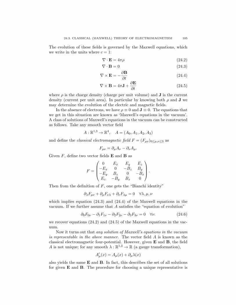
24.3. CLASSICAL (MAXWELL) THEORY OF ELECTROMAGNETISM 105
The evolution of these fields is governed by the Maxwell equations, whichwe write in the units where c = 1:
∇ ·E = 4πρ (24.2)
∇ ·B = 0 (24.3)
∇×E = −∂B
∂t(24.4)
∇×B = 4πJ +∂E
∂t(24.5)
where ρ is the charge density (charge per unit volume) and J is the currentdensity (current per unit area). In particular by knowing both ρ and J wemay determine the evolution of the electric and magnetic fields.
In the absence of electrons, we have ρ ≡ 0 and J ≡ 0. The equations thatwe get in this situation are known as ‘Maxwell’s equations in the vacuum’.A class of solutions of Maxwell’s equations in the vacuum can be constructedas follows. Take any smooth vector field
A : R1,3 → R4, A = (A0, A1, A2, A3)
and define the classical electromagnetic field F = (Fµν)0≤µ,ν≤3 as
Fµν = ∂µAν − ∂νAµ.Given F , define two vector fields E and B as
F =
0 Ex Ey Ez−Ex 0 −Bz By−Ey Bz 0 −BxEz −By Bx 0
.
Then from the definition of F , one gets the “Bianchi identity”
∂λFµν + ∂µFνλ + ∂νFλµ = 0 ∀λ, µ, νwhich implies equation (24.3) and (24.4) of the Maxwell equations in thevacuum. If we further assume that A satisfies the “equation of evolution”
∂0F0ν − ∂1F1ν − ∂2F2ν − ∂3F3ν = 0 ∀ν. (24.6)
we recover equations (24.2) and (24.5) of the Maxwell equations in the vac-uum.
Now it turns out that any solution of Maxwell’s equations in the vacuumis representable in the above manner. The vector field A is known as theclassical electromagnetic four-potential. However, given E and B, the fieldA is not unique; for any smooth λ : R1,3 → R (a gauge transformation),
A′µ(x) = Aµ(x) + ∂µλ(x)
also yields the same E and B. In fact, this describes the set of all solutionsfor given E and B. The procedure for choosing a unique representative is
106 24. THE ELECTROMAGNETIC FIELD
called gauge fixing. There are many ways to do this, but one way is toimpose the Lorenz gauge condition,
∂0A0 − ∂1A1 − ∂2A2 − ∂3A3 ≡ 0.
(Note that this ‘Lorenz’ without a ‘t’ — not the same as the Lorentz inLorentz transforms.)
24.4. From classical to quantized
The quantized electromagnetic four-potential A = (Aµ)0≤µ≤3 that wedefined using the Gupta–Bleuler approach is a quantization of the classi-cal electromagnetic four-potential, in the sense that it satisfies the vacuumMaxwell equations formally. Moreover, it also satisfies the Lorenz gaugecondition, in the sense that for any f ∈ S (R4),
∂0A0(f)− ∂1A1(f)− ∂2A2(f)− ∂3A3(f) = 0
as an operator on Bphys.
24.5. A note on the Einstein convention
Many of the expressions in this lecture could have been written muchmore compactly using Einstein’s conventions for special relativity. In par-ticular, there are two important rules:
• If we have a 4-tuple of objects (aµ)0≤µ≤3, then raising µ changes thesign of the last three. That is, a0 = a0, but a1 = −a1, a2 = −a2,and a3 = −a3. If the indices were raised to begin with, the loweringthem has the same effect. For example, we can raise the indices on∂µ to get ∂µ.• If an index is repeated within the same term, that indicates that
we have to sum over that index. For example,
∂µAµ =3∑
µ=0
∂µAµ = ∂0A0 − ∂1A1 − ∂2A2 − ∂3A3.
Thus, for example, the Lorenz gauge condition can be compactly writtenas ∂µAµ = 0. Similarly, the equation of motion (24.6) can be writtenas ∂µFµν = 0 for each ν. The expression (24.1) becomes Aµ(fµ). TheMinkowski inner product between x, y ∈ R1,3 is xµyµ.

LECTURE 25
The model for free electrons
Date: 11/28/2018Scribe: Kevin Yang
25.1. Projective representations
Today, we will construct a model for electrons that also applies forpositrons and several other types of particles. Let m equal the rest massof the electron. Let H = L2(Xm, dλm,C2) be the space of C2-valued L2-functions on the manifold Xm under the measure dλm. The spacetime stateof an electron is described by an element of this space. There are two basicquestions to answer before we proceed any further:
(1) What is the inner product on this space?(2) What is the representation of the Poincare group, P?
To answer the second question, we need to modify the fifth postulate ofquantum field theory stated in Lecture 11. Recall that this postulate statesthat if a system looks like it is in state ψ ∈ H in some choice of coordinatesystem, then upon changing the coordinate system by some (a,A) ∈ P,the system looks like it is in the state U(a,A)ψ, where U is some uni-tary representation of P in H. The representation property ensures thatU((a,A)(b, B)) = U(a,A)U(b, B), meaning that two successive changes ofcoordinate system amount to one composite change, and unitarity ensuresthat normalized states are sent to normalized states (conservation of prob-ability). Now note that expectations of observables under a state ψ areinvariant under multiplication of the state by a phase α ∈ C, |α| = 1. Thus,we do not really need U two a unitary representation; it suffices that U isunitary and is a projective representation, meaning that
U((a,A), (b, B)) = r(a,A, b, B)U(a,A)U(b, B),
where r(a,A, b, B) ∈ C and |r(a,A, b, B)| = 1.
25.2. The representation for electrons
Let SL(2,C) be the group of 2 × 2 complex matrices of determinant 1.For any point x ∈ R1,3, define the matrix
M(x) =
(x0 + x3 x1 − ix2
x1 + ix2 x0 − x3
).
107

108 25. THE MODEL FOR FREE ELECTRONS
One can check the above definition provides a bijection between R1,3 andthe space of 2× 2-complex Hermitian matrices. Moreover,
detM(x) = (x, x),
where the bracket on the right is the Minkowski inner product.Now take any A ∈ SL(2,C). Then for any x ∈ R1,3, the matrix
AM(x)A† is again a 2× 2 complex Hermitian matrix. Define κ(A)(x) to bethe unique y ∈ R1,3 such that
M(y) = AM(x)A†.
The following facts about κ are not hard to prove:
• For any A ∈ SL(2,C), κ(A) is a linear map on R1,3.• κ is a 2-to-1 surjective homomorphism from SL(2,C) onto SO↑(1, 3).• κ(A) = κ(B) if and only if either A = B or A = −B. (We will
henceforth write this as A = ±B.)• κ(A†) = κ(A)†, where M † denotes the conjugate transpose of a
matrix M .
By the second property listed above, there are many maps ρ : SO↑(1, 3)→SL(2,C) such that κ % is the identity on SO↑(1, 3). Moreover, any such %satisfies %(AB) = ±%(A)%(B). It turns out that due to algebraic constraints,we cannot choose % to be a homomorphism. The fourth property impliesthat %(A†) = ±%(A)†.
25.3. Constructing the inner product
We assume that nature provides a % as above so that the projectiverepresentation of SO↑(1, 3) in the space H = L2(Xm, dλm,C2) is given by
(U(a,A)ψ)(p) = ei(a,p)%(A)ψ(A−1p).
One can check that this is inded a projective representation. To prove thatthe above representation is unitary, we first have to define the inner product.We now build the inner product on H. Let p∗ = (m, 0, 0, 0) ∈ Xm denote adistinguished element of the manifold Xm. The action of SO↑(1, 3) on Xm
is transitive, so for any p ∈ Xm there are maps taking p∗ to p. If A, B areany such maps, then they are related by a spatial rotation:
A = BR, R =
(1 00 Q
), Q ∈ SO(3).
In words, R fixes time and acts by rotation on the spatial variables. Itturns out that there exists a standard way to choose a unique element fromthe class of all such maps taking p∗ to p. Precisely, for any p ∈ Xm thereexists a unique positive-definite Vp ∈ SL(2,C) such that κ(Vp)(p
∗) = p. Theuniqueness is provided by the positive-definite constraint. In the physicsliterature, the map κ(Vp) is known as the “pure boost” that takes p∗ to p.

25.4. FERMIONIC FOCK SPACE 109
With this machinery in place, we may now define the following innerproduct on H:
(ψ,ϕ) :=
∫Xm
dλm(p)ψ(p)†V −2p ϕ(p), ψ, ϕ ∈ L2(Xm, dλm,C2).
It is not difficult to verify that H is indeed a Hilbert space under this innerproduct. We now need to check that, under this inner product, the projectiverepresentation U is unitary. To this end, we first note
(U(a,A)ψ)(p)†V −2p (U(a,A)ϕ)(p) = ψ(A−1p)†%(A)†V −2
p %(A)ϕ(A−1p).
Integrating the right side with respect to dλm on Xm, we get
(U(a,A)ψ,U(a,A)ϕ) =
∫Xm
dλm(p)ψ(p)†%(A)†V −2Ap %(A)ϕ(p)
by the Lorentz invariance of dλm. It now remains to prove the followingidentity.
Lemma 25.1. For any A and p,
%(A)†V −2Ap %(A) = V −2
p .
Proof. Since κ is a homomorphism, we know
κ(V −1Ap %(A)) = κ(V −1
Ap )κ(%(A)) = κ(VAp)−1A.
By definition of V , we know
A−1κ(VAp)p∗ = A−1Ap = p.
Thus, A−1κ(VAp) = κ(Vp)R for some spatial rotation R. Applying % to bothsides, we get
%(A)−1VAp = ±Vp%(R).
This, in turn, implies
%(A)†V −2Ap %(A) = V −1
p (%(R)−1)†%(R)−1V −1p = ±V −2
p ,
since %(R)%(R)† = ±%(RR†) = ±I. But %(A)†V −2Ap %(A) and V −2
p are bothpositive definite matrices, and therefore they must be equal. This completesthe proof.
25.4. Fermionic Fock Space
We have now built the state space for a single electron. Because electronsare fermionic in nature, to build the state space for n electrons we need tobuild a fermonic Fock space instead of the bosonic Fock space. This isdefined as follows.

110 25. THE MODEL FOR FREE ELECTRONS
Let H denote the Hilbert space for a single fermionic particle. Letej∞j=1 be an orthonormal basis of H. The appropriate state space forn such particles is
H⊗nanti =
∑i1,...,in≥1
αi1,...,inei1 ⊗ . . .⊗ ein : ∀σ ∈ Sn,
αiσ(1),...,iσ(n) = sign(σ)αi1,...,in
.
With αi1,...,in as above, note that αi1,...,in = 0 if i1, . . . , in are not distinctindices. Indeed, if we had a pair of repeated indices, the transposition swap-ping their positions would preserve the index-tuple. Since transpositions areodd, this would imply αi1,...,in = −αi1,...,in .
Like the bosonic versions, these spaces are actually basis-independent.We now define
F0 =∞⊕n=0
H⊗nanti,
and let F denote the closure of F0 under the natural inner product. In thecontext of electrons, we will take H = L2(Xm, dλm,C2), and the state spacefor arbitrary numbers of electrons to be the fermionic Fock space of H.
We conclude with a simple example. If H = L2(R), then the fermionicFock space of n particles is
H⊗nanti =
f ∈ L2(Rn) : f(xσ(1), . . . , xσ(n)) = sign(σ)f(x1, . . . , xn),
∀x ∈ Rn, ∀σ ∈ Sn.

LECTURE 26
The Dirac field
Date: 11/30/2018Scribe: Cole Graham
26.1. A basis for fermionic Fock space
Given an orthonormal basis e1, e2, . . . of H, we can form an orthonormalbasis for H⊗nanti from elements of the form
1√n!
∑σ∈Sn
sgn(σ)eiσ(1) ⊗ · · · ⊗ eiσ(n) ,
where i1 < i2 < · · · < in. We denote this element by |n1, n2, . . .〉, where
nj =
1 if j ∈ i1, . . . , in,0 otherwise.
We may interpret the multi-particle state |n1, . . .〉 as n particles in statesei1 , . . . , ein . As remarked in the previous lecture, the antisymmetry forbidsoccupation numbers above 1. This is the Pauli exclusion principle: twoidentical fermions cannot simultaneously occupy the same state.
From the above discussion, we have that|n1, n2, . . .〉 : ni ∈ 0, 1 and
∑i
ni = n
is an orthonormal basis for H⊗nanti. Allowing n to vary in Z≥0, we obtain anorthonormal basis for the fermionic Fock space F :
|n1, n2, . . .〉 : ni ∈ 0, 1 and∑i
ni <∞.
26.2. Creation and annihilation operators on FWe begin by defining creation and annihilation operators relative to a
fixed orthonormal basis ei of H. For each k ≥ 1, define the creation
operator a†k as follows. Let ψ = |n1, n2, . . .〉. If nk = 1, let a†kψ = 0, where0 denotes the zero of the vector space F , not the vacuum state. If insteadnk = 0, let
a†kψ = (−1)m |n1, . . . , nk−1, 1, nk+1, . . .〉 ,111
112 26. THE DIRAC FIELD
where
m := #1 ≤ i < k : ni = 1 =k−1∑i=1
ni.
Remark 26.1. If ψ = |0, 0, . . .〉 is the vacuum state, a†kψ is the statewith one particle in state ek, as expected.
We also have an annihilation operator ak. If nk = 0, let akψ = 0. Ifinstead nk = 1, let
akψ = (−1)m |n1, . . . , nk−1, 0, nk+1, . . .〉 ,
with m as above. The sign correction (−1)m will ensure simpler formulæ inthe sequel.
We now define continuous versions of a†k and ak. We want maps A† andA from H into L (F0,F), where L (F0,F) denotes the space of linear mapsfrom F0 to F . Given f ∈ H, write
f =∞∑k=1
αkek
and define
A†(f)ψ :=∑k
αka†kψ, A(f)ψ :=
∑k
α∗kakψ.
Remark 26.2. Although we do not show it here, A†, A are basis inde-pendent. That is, they do not depend on the choice of basis ei for H.
We can easily check the following anticommutation relations:
ak, a†` = δk,`1, a†k, a†` = 0, ak, a` = 0 for all k, ` ∈ N.
Here A,B := AB+BA is the anticommutator of A and B. These relationsimply
A(ξ), A†(η) = (ξ, η)1, A†(ξ), A†(η) = 0, A(ξ), A(η) = 0
for all ξ, η ∈ H.Now if U is a unitary operator on H, it has a natural extension to F (by
acting on each factor in an elementary tensor). As in the bosonic case, wehave
UA(ξ)U−1 = A(Uξ) and UA†(ξ)U−1 = A†(Uξ) for all ξ ∈ H.
An analog of Wick’s theorem holds in the fermionic case, with one wrinkle:the resulting sum is signed.
26.3. THE DIRAC FIELD 113
26.3. The Dirac field
Recall that massive scalar bosons have a corresponding free field, andphotons the electromagnetic field. We now define the Dirac field associatedto electrons (and all spin-1
2 particles).Let m denote the mass of the electron. In the last lecture, we defined the
single-electron state-space H = L2(Xm,dλm,C2), and endowed it with aninner product based on our projective representation of the Poincare group.Let F denote the fermionic Fock space corresponding to H, and let e1, e2
denote the standard basis vectors of C2.We will formally define operator-valued distributions a†(p, s) and a(p, s)
for p ∈ Xm and s ∈ 1, 2. For ξ ∈ L2(Xm,dλm), we say
A†(ξes) =
∫Xm
dλm(p) ξ(p)a†(p, s)
A(ξes) =
∫Xm
dλm(p) ξ(p)∗a(p, s).
Thus formally
a†(p, s) = A†(δpes) and a(p, s) = A(δpes).
This is wholly analogous to the case of scalar bosons.Recall that Xm is parameterized by p ∈ R3 with p = (p0,p) and p0 =
ωp :=√m2 + p2. We define
a†(p, s) :=a†(p, s)√
2ωpand a(p, s) :=
a(p, s)√2ωp
.
Then we can check that
a(p, s), a†(p′, s′) = (2π)3δ(3)(p− p′)δs,s′1,
and all other anticommutators vanish. Again, these are much like the com-mutator relations in the scalar boson case.
Now recall our distinguished element p∗ = (m, 0, 0, 0) ∈ Xm. For eachp ∈ Xm, recall that there is a unique positive-definite Vp ∈ SL(2,C) suchthat
κ(Vp)p∗ = p.
Here κ : SL(2,C) → SO↑(1, 3) denotes the double-cover defined in the pre-vious lecture. The transformation κ(Vp) is the “pure boost” that takes p∗
to p. Define Sp ∈ GL(4,C) by
Sp :=
((V †p )−1 0
0 Vp
).

114 26. THE DIRAC FIELD
Also, define a basis f1, f2, f′1, f′2 of C4:
f1 :=
1010
, f2 :=
0101
, f ′1 :=
10−10
, f ′2 :=
010−1
.
Finally, define
u(p, s) := Spfs and v(p, s) := Spf′s. (26.1)
Let uk, vk denote the components of u, v for k ∈ 1, 2, 3, 4.We have defined F to be the fermionic Fock space for electrons. Con-
struct an identical copy F ′ for positrons. Then let G := F ⊗ F ′ denote thejoint electron-positron space. Let b† and b denote the analogs of a† and aon F ′. Note that any operator C on F extends uniquely to G via
C(f ⊗ f ′) := Cf ⊗ f ′.Operators likewise extend from F ′ to G.
For each k ∈ 1, 2, 3, 4, we formally define an operator-valued distribu-tion ψk on R1,3 as
ψk(x) :=2∑s=1
∫R3
d3p
(2π)3
√m√
2ωp
[e−i(x,p)uk(p, s)a(p, s)
+ ei(x,p)vk(p, s)b†(p, s)
]. (26.2)
We then form the 4-tuple of operator valued distributions
ψ(x) :=
ψ1(x)ψ2(x)ψ3(x)ψ4(x)
.
We should consider how ψ differs from the free field ϕ. Of course ψ has fourcomponents, sums over the two spins s = 1, 2, and involves factors u and vfrom the projective representation. Most importantly, however, ψ involvesa and b† rather than simply a and a†. Early attempts to treat electronsran into inconsistencies when using just F . Dirac had the insight to addan extra Fock space F ′, which resolved all difficulties in the theory. Indeed,the strength of the theory led Dirac to predict the existence of the positronbefore its experimental discovery.
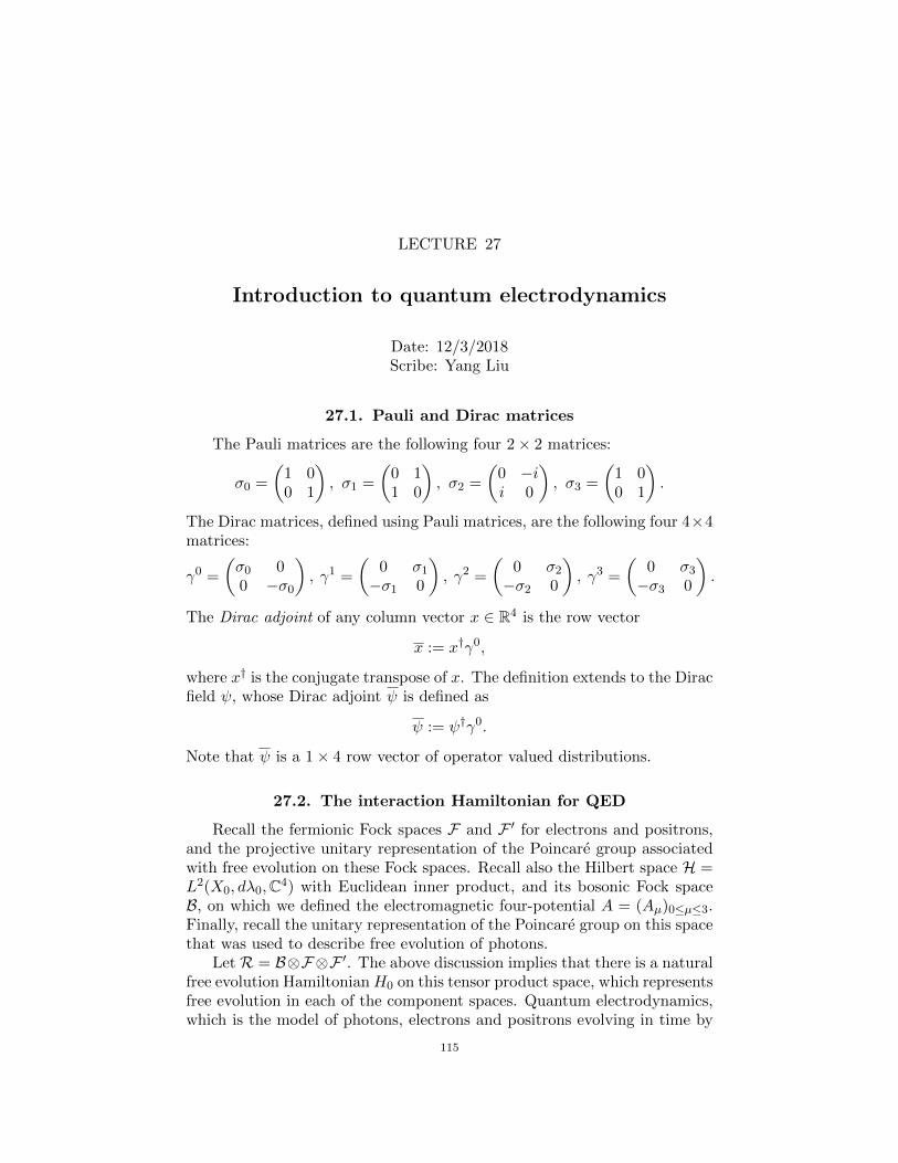
LECTURE 27
Introduction to quantum electrodynamics
Date: 12/3/2018Scribe: Yang Liu
27.1. Pauli and Dirac matrices
The Pauli matrices are the following four 2× 2 matrices:
σ0 =
(1 00 1
), σ1 =
(0 11 0
), σ2 =
(0 −ii 0
), σ3 =
(1 00 1
).
The Dirac matrices, defined using Pauli matrices, are the following four 4×4matrices:
γ0 =
(σ0 00 −σ0
), γ1 =
(0 σ1
−σ1 0
), γ2 =
(0 σ2
−σ2 0
), γ3 =
(0 σ3
−σ3 0
).
The Dirac adjoint of any column vector x ∈ R4 is the row vector
x := x†γ0,
where x† is the conjugate transpose of x. The definition extends to the Diracfield ψ, whose Dirac adjoint ψ is defined as
ψ := ψ†γ0.
Note that ψ is a 1× 4 row vector of operator valued distributions.
27.2. The interaction Hamiltonian for QED
Recall the fermionic Fock spaces F and F ′ for electrons and positrons,and the projective unitary representation of the Poincare group associatedwith free evolution on these Fock spaces. Recall also the Hilbert space H =L2(X0, dλ0,C4) with Euclidean inner product, and its bosonic Fock spaceB, on which we defined the electromagnetic four-potential A = (Aµ)0≤µ≤3.Finally, recall the unitary representation of the Poincare group on this spacethat was used to describe free evolution of photons.
Let R = B⊗F⊗F ′. The above discussion implies that there is a naturalfree evolution HamiltonianH0 on this tensor product space, which representsfree evolution in each of the component spaces. Quantum electrodynamics,which is the model of photons, electrons and positrons evolving in time by
115
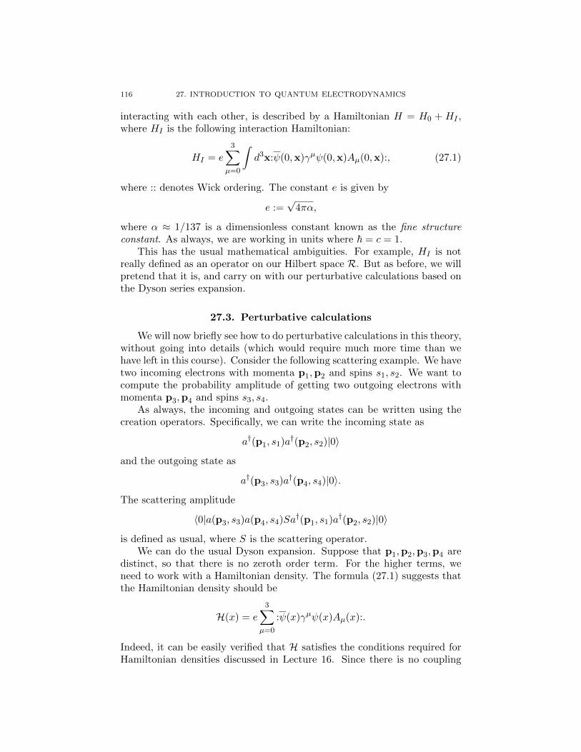
116 27. INTRODUCTION TO QUANTUM ELECTRODYNAMICS
interacting with each other, is described by a Hamiltonian H = H0 + HI ,where HI is the following interaction Hamiltonian:
HI = e3∑
µ=0
∫d3x:ψ(0,x)γµψ(0,x)Aµ(0,x):, (27.1)
where :: denotes Wick ordering. The constant e is given by
e :=√
4πα,
where α ≈ 1/137 is a dimensionless constant known as the fine structureconstant. As always, we are working in units where ~ = c = 1.
This has the usual mathematical ambiguities. For example, HI is notreally defined as an operator on our Hilbert space R. But as before, we willpretend that it is, and carry on with our perturbative calculations based onthe Dyson series expansion.
27.3. Perturbative calculations
We will now briefly see how to do perturbative calculations in this theory,without going into details (which would require much more time than wehave left in this course). Consider the following scattering example. We havetwo incoming electrons with momenta p1,p2 and spins s1, s2. We want tocompute the probability amplitude of getting two outgoing electrons withmomenta p3,p4 and spins s3, s4.
As always, the incoming and outgoing states can be written using thecreation operators. Specifically, we can write the incoming state as
a†(p1, s1)a†(p2, s2)|0〉and the outgoing state as
a†(p3, s3)a†(p4, s4)|0〉.The scattering amplitude
〈0|a(p3, s3)a(p4, s4)Sa†(p1, s1)a†(p2, s2)|0〉is defined as usual, where S is the scattering operator.
We can do the usual Dyson expansion. Suppose that p1,p2,p3,p4 aredistinct, so that there is no zeroth order term. For the higher terms, weneed to work with a Hamiltonian density. The formula (27.1) suggests thatthe Hamiltonian density should be
H(x) = e
3∑µ=0
:ψ(x)γµψ(x)Aµ(x):.
Indeed, it can be easily verified that H satisfies the conditions required forHamiltonian densities discussed in Lecture 16. Since there is no coupling
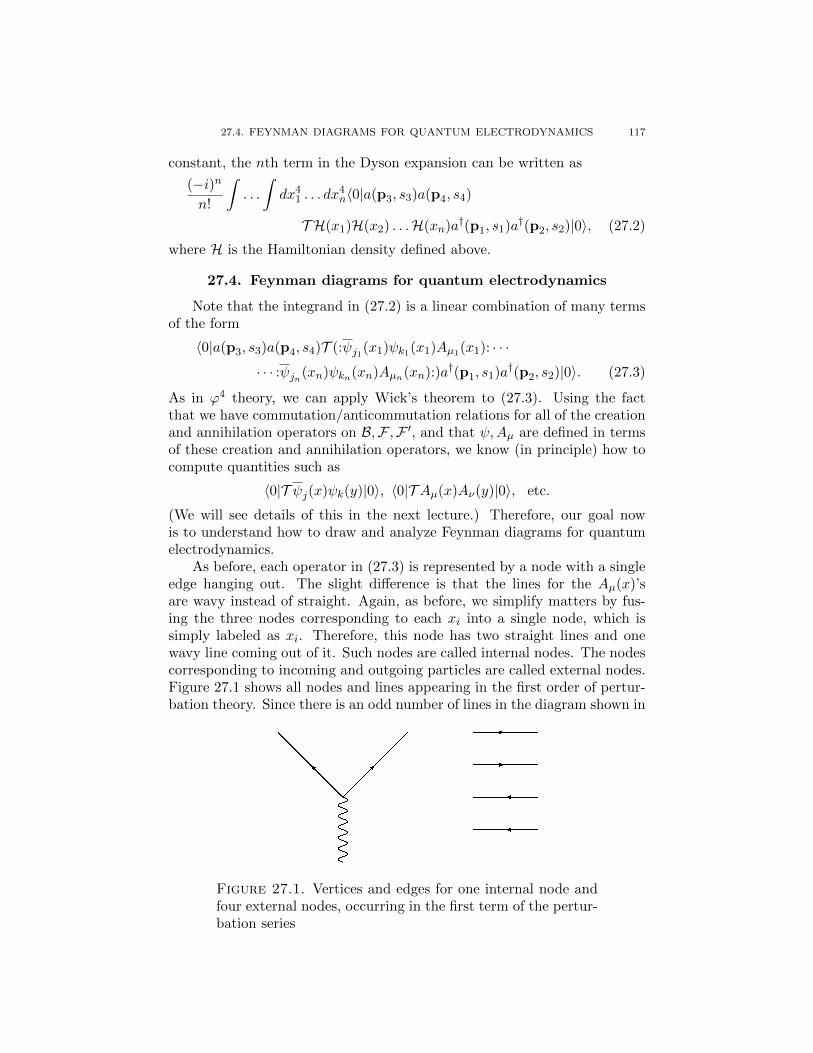
27.4. FEYNMAN DIAGRAMS FOR QUANTUM ELECTRODYNAMICS 117
constant, the nth term in the Dyson expansion can be written as
(−i)nn!
∫. . .
∫dx4
1 . . . dx4n〈0|a(p3, s3)a(p4, s4)
T H(x1)H(x2) . . .H(xn)a†(p1, s1)a†(p2, s2)|0〉, (27.2)
where H is the Hamiltonian density defined above.
27.4. Feynman diagrams for quantum electrodynamics
Note that the integrand in (27.2) is a linear combination of many termsof the form
〈0|a(p3, s3)a(p4, s4)T (:ψj1(x1)ψk1(x1)Aµ1(x1): · · ·· · · :ψjn(xn)ψkn(xn)Aµn(xn):)a†(p1, s1)a†(p2, s2)|0〉. (27.3)
As in ϕ4 theory, we can apply Wick’s theorem to (27.3). Using the factthat we have commutation/anticommutation relations for all of the creationand annihilation operators on B,F ,F ′, and that ψ,Aµ are defined in termsof these creation and annihilation operators, we know (in principle) how tocompute quantities such as
〈0|T ψj(x)ψk(y)|0〉, 〈0|T Aµ(x)Aν(y)|0〉, etc.
(We will see details of this in the next lecture.) Therefore, our goal nowis to understand how to draw and analyze Feynman diagrams for quantumelectrodynamics.
As before, each operator in (27.3) is represented by a node with a singleedge hanging out. The slight difference is that the lines for the Aµ(x)’sare wavy instead of straight. Again, as before, we simplify matters by fus-ing the three nodes corresponding to each xi into a single node, which issimply labeled as xi. Therefore, this node has two straight lines and onewavy line coming out of it. Such nodes are called internal nodes. The nodescorresponding to incoming and outgoing particles are called external nodes.Figure 27.1 shows all nodes and lines appearing in the first order of pertur-bation theory. Since there is an odd number of lines in the diagram shown in
Figure 27.1. Vertices and edges for one internal node andfour external nodes, occurring in the first term of the pertur-bation series
118 27. INTRODUCTION TO QUANTUM ELECTRODYNAMICS
Figure 27.1, it is impossible to tie them without leaving at least one untiedline. Therefore the first-order term is zero.
Let us next look at the second order term. The set of all nodes and linesfor this term is shown in Figure 27.2. In this case it is in fact possible to
Figure 27.2. Vertices and edges for two internal nodes andfour external nodes, occurring in the second term of the per-turbation series
tie up all lines so that no line remains untied. The Wick ordering in theHamiltonian density ensures that diagrams with self-loops at internal nodesdo not contribute. A typical example of a contributing diagram is shown inFigure 27.3. Physically, it corresponds to two incoming electrons exchanginga photon and scattering into two outgoing electrons.
Figure 27.3. Example of a matching of 6 lines: 4 corre-sponding to electrons and 2 to photons
In fact, this is the only kind of diagram that contributes. The reason isas follows. From all the considerations mentioned above, the other kind ofdiagram that could have contributed are diagrams where the two incomingelectron lines meet at one internal node, and the two outgoing electronlines meet at the other internal node. However, such diagrams give zerocontribution, because
〈0|a(p, s)ψk(x)|0〉 = 0
for any p, s, k and x, as is apparent from the definition (26.2) of ψk(x) andthe facts that 〈a(p, s)a(p′, s′)|0〉 = 0 and 〈0|a(p, s)b†(p′, s′)|0〉 = 0 for anyp, s, p′ and s′.
LECTURE 28
Electron scattering
Date: 12/5/2018Scribe: Cyrus Reza
28.1. The Dirac propagator
In this lecture, we will briefly outline a calculation in QED without goinginto the details of all the steps. Recall that we are trying to compute thesecond order term in the Dyson expansion for the scattering amplitude
〈0|a(p3, s3)a(p4, s4)Sa†(p1, s1)a†(p2, s2)|0〉 (28.1)
of getting two outgoing electrons with momenta p3, p4 and spins s3, s4,from two incoming electrons with momenta p1, p2 and spins s1, s2. Wehave argued that the only type of Feynman diagram that contributes to thiscalculation are diagrams of the type shown in Figure 27.3.
To compute the contribution of any internal line in QED, we need tocalculate two kinds of propagators in QED, akin to the Feynman propagatorappearing in ϕ4 scalar field theory. Recall that the Feynman propagator fora particle of mass m is given by
∆F,m(x) = limε→0
∫d4p
(2π)4
e−i(x,p)
−p2 +m2 − iε .
(We were writing it earlier as ∆F , but we will need to be explicit aboutm here.) The Dirac propagator is a 4 × 4 array of Schwartz distributions,defined as
∆D(x) =3∑
µ=0
(i∂µ∆F,m(x))γµ +m∆F,m(x)I,
where γµ are the Dirac matrices defined in the previous lecture, and I is the4 × 4 identity matrix. The Dirac propagator appears in QED calculationsin the following way. For any 1 ≤ j, k ≤ 4,
〈0|T ψj(x1)ψk(x2)|0〉 = −〈0|T ψj(x1)ψk(x2)|0〉 = −i(∆D(x1 − x2))jk.
This kind of internal line does not, however, appear in Figure 27.3, but doappear in higher orders of perturbation theory.
119

120 28. ELECTRON SCATTERING
28.2. The photon propagator
The photon propagator ∆µν , for 0 ≤ µ, ν ≤ 3, is defined as
∆µν(x) = −ηµν∆F,0(x),
where ∆F,0 is the Feynman propagator with m = 0, and as usual,
η =
1 0 0 00 −1 0 00 0 −1 00 0 0 −1
.
The photon propagator appears in QED calculations in the following way.For any 0 ≤ µ, ν ≤ 3,
〈0|T Aµ(x1)Aν(x2)|0〉 = −i∆µν(x1 − x2).
28.3. Second order term in electron scattering
The Dirac propagator and the photon propagator allow us to calculatethe contributions of the internal lines in Feynman diagrams for QED. Con-tributions from external lines, which are of the form 〈0|ψk(x)a†(p, s)|0〉, etc.,can be calculated using commutation relations for the creation and annihi-lation operators. Without going into details, let us just mention that theend result of such calculations show that the second order term in the Dysonexpansion of (28.1) is
3∑µ,ν=0
im2e2√16ωp1
ωp2ωp3
ωp4
u(p3, s3)γµu(p1, s1)ηµν
(p3 − p1)2u(p4, s4)γνu(p2, s2)
+ similar terms,
where u(p, s) is the Dirac adjoint of the vector u(p, s) defined in (26.1), andthe “similar terms” are obtained by exchanging p3 with p4, and p1 with p2.
28.4. The non-relativistic limit
Let us now consider the non-relativistic limit of the scattering amplitudecomputed above, that is, where |pi| 1 for each i. In this situation, wehave ωpi ≈ m for each i. We also have
(p3 − p1)2 = (p03 − p0
1)2 − (p3 − p2)2,
and
p0i =
√m2 + p2
i ≈ m+p2i
m,
which implies that
(p3 − p1)2 = −(p3 − p1)2(1 + o(1)).
Lastly,
u(p, s)γµu(p′, s′) ≈ u(0, s)γµu(0, s′),
28.5. ANOMALOUS MAGNETIC MOMENT OF THE ELECTRON 121
and the right side, when summed over µ, gives 2δs,s′ . Therefore in thenon-relativistic limit, the second order term in the scattering amplitude isapproximately equal to
−ie2
(p3 − p1)2δs1,s3δs2,s4(2π)4δ(4)(p3 + p4 − p1 − p2) + similar terms.
The function V : R3 → R whose Fourier transform is
V (p) =1
p2
is the function
V (x) =1
4π|x| .This indicates that if we assumed a non-relativistic quantum mechanicalmodel for electrons and used the Coulomb potential to model the repulsionbetween electrons, we would have ended up with the same scattering ampli-tude. Thus, the Coulomb potential arises naturally in the non-relativisticlimit of QED.
28.5. Anomalous magnetic moment of the electron
The anomalous magnetic moment of the electron is a dimensionlessquantity, predicted to be equal to 1 by non-relativistic quantum mechanics(~ = c = 1). The experimental value deviates slightly from this prediction.Currently, the experimentally determined value, up to ten places of decimal,is the following:
1.001 159 652 180 73(±28).
It is one of the great successes of QED that it gives a much more accurateprediction for this quantity. The theoretical value, when calculated usingsecond order perturbation theory, already gives
1.001 161 4.
However, when one goes to fifth order of perturbation theory, one gets
1.001 159 652 181 643(±764),
which is a truly astonishing match with experiment, unparalleled in all ofscience.


LECTURE 29
The Wightman axioms
Date: 12/7/2018Scribe: Chenyang Zhong
29.1. Interacting quantum fields
Until now, we have only worked with free fields, and scattering ampli-tudes computed using free fields. There are, however, important objectsknown as interacting quantum fields that are more complicated than freefields. Let us now see the simplest example of an interacting quantum field.Recall ϕ4 theory. We have the Hilbert space H = L2(Xm, dλm) and thescalar free field ϕ. In this lecture, we will denote the free field by ϕfree, todistinguish it from the interacting field ϕ that we are going to define below.
Recall the Hamiltonian H = H0 + gHI , where H0 is the Hamiltonian offree evolution, and
HI =1
4!
∫d3x:ϕfree(0,x)4:.
The interacting field ϕ defined by the Hamiltonian H is
ϕ(t,x) := eitHϕfree(0,x)e−itH .
In particular, ϕ(0,x) = ϕfree(0,x). In other words, the interacting fieldstarts off as ϕfree at time zero, but then evolves according to the HamiltonianH instead of H0 (in the Heisenberg picture of evolution of operators). Incontrast, the free field evolves as
ϕfree(t,x) = eitH0ϕfree(0,x)e−itH0 ,
a fact that we have noted before.Note that the definition of ϕ does not make mathematical sense, since
H is not a mathematically well-defined operator on H. The rigorous defi-nition of interacting quantum fields is one of the major open questions inmathematical physics. We will discuss one approach to the solution of thisquestion below.
29.2. Green’s functions
Suppose that H is indeed a well-define operator (possibly on a space thatis different than H), and that it has a unique ground state (i.e. an eigenstatewith minimum eigenvalue) Ω. This is called the vacuum state of the theory.
123

124 29. THE WIGHTMAN AXIOMS
Note that Ω 6= |0〉. The Green’s functions (or Schwinger functions) for thetheory are defined, for each n, as
G(x1, . . . , xn) = 〈Ω|T ϕ(x1) · · ·ϕ(xn)|Ω〉 (29.1)
where x1, . . . , xn ∈ R1,3.Typically, G is expected to be a distribution rather than a function.
It turns out that the Green’s functions contain much more informationthan scattering amplitudes. In particular, scattering amplitudes can berecovered from the Green’s functions using the LSZ (Lehmann–Symanzik–Zimmermann) formula. The Green’s functions for an interacting theory arecomputed using the free field and the Gell-Mann–Low theorem.
29.3. The Wightman axioms
The Wightman axioms give a framework for rigorously defining inter-acting quantum field theories. The axioms are designed to ensure that thereare no physical inconsistencies. Let us only consider the axioms for bosonicscalar fields for now.
Axiom 1. There exists a Hilbert space H whose elements represent thepossible states of the quantum system under consideration, and a unitaryrepresentation U of P in H. (We do not need “projective” because we aredealing with scalar fields.) There is one further assumption about U , and itneeds a bit of preparation to state. Note that (U(a, 1))a∈R1,3 is a commut-ing family of unitary operators. Therefore by the spectral theorem, we havethat
U(a, 1) =
∫R1,3
dE(p)ei(a,p),
where E is a projection-valued measure on R1,3. Let
L := p ∈ R1,3 : p0 ≥ |p|be the “forward light cone”. The additional assumption on U is that
E(A) = 0 whenever A ∩ L = ∅.This assumption is required to ensure that there are no particles with “neg-ative masses” in the theory. There is a simple way to check (29.3). Thecondition is satisfied if and only if for any ξ, η ∈ H and any f ∈ S (R1,3),
such that the support of f does not intersect L, we have∫d4af(a)(ξ, U(a, 1)η) = 0.
Axiom 2. There exists a dense subspace D of H and a linear map
ϕ : S (R4)→ unbounded operators on H

29.4. THE PROBABILISTIC APPROACH 125
such that for f ∈ S (R4), we have that ϕ(f) is defined on D and ϕ(f)(D) ⊂D. Moreover, we assume that for any ξ, η ∈ D,
(ϕ(f∗)ξ, η) = (ξ, ϕ(f)η).
In particular if f is real-valued, then ϕ(f) is a symmetric operator on D.
Axiom 3. For any ξ, η ∈ D, f 7→ (ξ, ϕ(f)η) is a tempered distribution.
Axiom 4. For any (a,A) ∈ P,
U(a,A)ϕ(f)U(a,A)−1 = ϕ(V (a,A)f),
where
V (a,A)f(x) = f(A−1(x− a)).
This is the axiom of Lorentz invariance, designed to ensure compatibilitywith special relativity.
Axiom 5. If the supports of f, g ∈ S (R4) are “spacelike separated”, then
[φ(f), φ(g)] = 0.
(Two points x, y ∈ R1,3 are called spacelike separated if (x− y)2 < 0. Twosets are spacelike separated if any point in one spacelike separated fromany point in the other.) This is the locality axiom, designed to ensurecompatibility with the stipulation of special relativity that a signal cannottravel faster than the speed of light.
Axiom 6. There exists Ω ∈ D such that U(a, 1)Ω = Ω for any a, and it isthe unique element satisfying this condition. (One can actually deduce fromthe axioms that U(a,A)Ω = Ω for any (a,A) ∈ P.) This is the axiom thatensures the existence and uniqueness of the vacuum state.
Axiom 7. The closed linear span of elements like ϕ(f1) · · ·ϕ(fn)Ω for nand f1, . . . , fn arbitrary, is the Hilbert space H. This axiom is designed toensure that the field ϕ is “rich enough” to generate all possible states.
It can be verified that the scalar free field satisfies all of the above axioms.A quantum field theory ϕ is called interacting if it is not the free field. TheWightman axioms have analogs in R1,1 and R1,2, where interacting fieldssatisfying these axioms have been constructed. Unfortunately, no one hasbeen able to construct an interacting quantum field theory in R1,3 thatsatisfies the Wightman axioms.
29.4. The probabilistic approach
There is a probabilistic approach to the construction of interacting quan-tum field theories that satisfy the Wightman axioms. Suppose that we start

126 29. THE WIGHTMAN AXIOMS
with the Green’s function G(x1, . . . , xn) = G((t1,x1), . . . , (tnxn)) for a hy-pothetical quantum field theory, and analytically analytically continue it intime to get
S(x1, . . . , xn) := G((it1,x1), . . . , (itn,xn)).
From the path integral heuristic (which we have not discussed), it is expectedthat S is the n-point correlation function of a random field:
S(x1, . . . , xn) = E(ψ(x1) · · ·ψ(xn)),
where ψ is a random field on R1,3. Usually the field ψ is so rough that Sis still a distribution rather than a function. The correct random field canbe identified using the Lagrangian of the theory (again, which we have notdiscussed).
Once the guess about the random field has been made, one can try toverify that it satisfies a set of axioms known as the Osterwalder–Schraderaxioms. If these axioms are satisfied by ψ, then there exists a “reconstructiontheorem” that reconstructs the quantum field whose Green’s function G isthe analytic continuation of S in time. Here reconstructing the quantumfield means constructing a quantum field theory satisfying the Wightmanaxioms.
Using this approach, interacting scalar ϕ4 quantum field theories havebeen constructed on R1,1 and R1,2, but not yet on R1,3.
Open problem 29.1. Construct an interacting scalar quantum fieldtheory on R1,3 that satisfies the Wightman axioms.


![Fast summation of divergent series and resurgent ... · in quantum mechanics [8,9], ϕ4 theory in QFT [10], quantum chromodynamics [11], string perturbation theory [12,13], and diagrammatic](https://img.pdfslide.us/doc/110x75/5f0a67d97e708231d42b79af/fast-summation-of-divergent-series-and-resurgent-in-quantum-mechanics-89.jpg)