Embed Size (px)
Citation preview
INTRODUCTION TO QUANTUM COMPUTING 1.
Jozef Gruska
Faculty of InformaticsBrno
Czech Republic
March 5, 2008
Quantum computing 1, 2 - Introduction, Bhubaneswar, School, March 2008
1. INTRODUCTION
In the first lecture we deal with reasons why to study quantumcomputing and with very basic experiments, principles,formalism and some basic outcomes of Quantum InformationProcessing and Communication.
We deal also, at the beginning, in some details, with classicalreversible computations, as a special case of quantumcomputation.
Jozef Gruska March 5, 2008 1
Quantum computing 1, 2 - Introduction, Bhubaneswar, School, March 2008
INTRODUCTORY OBSERVATIONS
In quantum computing we witness a merge of two of the most importantareas of science of 20th century: quantum physics and informatics.
This merge is bringing new aims, challenges and potentials for informaticsand also new approaches for physics to explore quantum world.
In spite of the fact that it is hard to predict particular impacts of quantumcomputing on computing in general, it is quite safe to expect that the mergewill lead to important outcomes.
Jozef Gruska March 5, 2008 2
Quantum computing 1, 2 - Introduction, Bhubaneswar, School, March 2008
A VIEW of HISTORY
19th century was mainly influenced by the first industrial revolutionthat had its basis in theclassical mechanicsdiscovered,formalized and developed in the 18th century.
20th century was mainly influenced by the second industrialrevolution that had its basis inelectrodynamicsdiscovered,formalized and developed in the 19th century.
21th century can be expected to be mainly developed byquantummechanics and informaticsdiscovered, formalized anddeveloped in the 20th century.
Jozef Gruska March 5, 2008 3
Quantum computing 1, 2 - Introduction, Bhubaneswar, School, March 2008
QUANTUM PHYSICS
is
is an excellent theoryto predict probabilities of quantum events.
Quantum physicsis an elegant and conceptually simple theory thatdescribes with astounding precision a large spectrum of the phenomena ofNature.
The predictions made on the base of quantum physics have beenexperimentally verified to 14 orders of precision. No conflict betweenpredictions of theory and experiments is known.
Without quantum physics we cannot explain properties of superfluids,functioning of laser, the substance of chemistry, the structure and function ofDNA, the existence and behaviour of solid bodies, color of stars, . . ..
Jozef Gruska March 5, 2008 4
Quantum computing 1, 2 - Introduction, Bhubaneswar, School, March 2008
QUANTUM PHYSICS — SUBJECT I
Quantum physics deals with fundamentals entities of physics —particles like
• protons, electrons and neutrons (from which matter is built);
• photons (which carry electromagnetic radiation) - they are theonly particles we can directly observe;
• various “elementary particles” which mediate otherinteractions of physics.
We call them particles in spite of the fact that some of theirproperties are totally unlike the properties of what we callparticles in our ordinary world.
Indeed, it is not clear in what sense these “particles” can besaid to have properties at all.
Jozef Gruska March 5, 2008 5
Quantum computing 1, 2 - Introduction, Bhubaneswar, School, March 2008
QUANTUM MECHANICS
is, in spite of its quality, from the point of view of explaining quantumphenomena, a very unsatisfactory theory.
Quantum mechanicsis a theory with either some hard to accept principles ora theory leading to mysteries and paradoxes.
Quantum theory seems to lead to philosophical standpoints that manyfind deeply unsatisfying.At best, and taking its descriptions at their most literal, it provides uswith a very strange view of the world indeed.At worst, and taking literally the proclamations of some of its mostfamous protagonists, it provides us with no view of the world at all.
Roger Penrose
Jozef Gruska March 5, 2008 6
Quantum computing 1, 2 - Introduction, Bhubaneswar, School, March 2008
You have nothing to do but mention the quantum theory,and people will take your voice for the voice of science, andbelieve anything
Bernard Shaw (1938)
Jozef Gruska March 5, 2008 7
Quantum computing 1, 2 - Introduction, Bhubaneswar, School, March 2008
WHAT QUANTUM PHYSICS TELL US?
Quantum physics
tells us
WHAT happens
but does not tell us
WHY it happens
and does not tell us either
HOW it happens
nor
HOW MUCH it costs
Jozef Gruska March 5, 2008 8
Quantum computing 1, 2 - Introduction, Bhubaneswar, School, March 2008
QUANTUM PHYSICS UNDERSTANDING
I am going to tell you what Nature behaves like......
However do not keep saying to yourself, if you can possiblyavoid it,
BUT HOW CAN IT BE LIKE THAT?
because you will get “down the drain” into a blind alley fromwhich nobody has yet escaped.
NOBODY KNOWS HOW IT CAN BE LIKE THAT.Richard Feynman (1965): The character of physical law.
Jozef Gruska March 5, 2008 9
Quantum computing 1, 2 - Introduction, Bhubaneswar, School, March 2008
QUANTUM MECHANICS - ANOTHER VIEW
•Quantum mechanics is not physics in the usual sense - it isnot about matter, or energy or waves, or particles - it is aboutinformation, probabilities, probability amplitudes andobservables, and how they relate to each other.
•Quantum mechanics is what you would inevitably come upwith if you would started from probability theory, and thensaid, let’s try to generalize it so that the numbers we used tocall ”probabilities” can be negative numbers.
As such, the theory could be invented by mathematicians inthe 19th century without any input from experiment. It wasnot, but it could have been (Aaronson, 1997).
Jozef Gruska March 5, 2008 10
Quantum computing 1, 2 - Introduction, Bhubaneswar, School, March 2008
WHY is QIPC so IMPORTANT?
There are five main reasons why QIPC is increasingly considered as of (very) largeimportance:
• QIPC is believed to lead to new Quantum Information ProcessingTechnology that could have deep and broad impacts.
• Several sciences and technology are approaching the point at which theybadly need expertise with isolation, manipulating and transmission ofparticles.
• It is increasingly believed that new, quantum information processingbased, understanding of (complex) quantum phenomena and systems canbe developed.
• Quantum cryptography seems to offer new level of security and be soonfeasible.
• QIPC has been shown to be more efficient in interesting/important cases.
• TCS and Information theory got new dimension and impulses.
Jozef Gruska March 5, 2008 11
Quantum computing 1, 2 - Introduction, Bhubaneswar, School, March 2008
WHY WE SHOULD TRY to have QUANTUM COMPUTERS?
When you try to reach for stars you may not quite get one, butyou won’t come with a handful of mud either.
Leo Burnett
Jozef Gruska March 5, 2008 12
Quantum computing 1, 2 - Introduction, Bhubaneswar, School, March 2008
WHY von NEUMANN
DID (COULD) NOT DISCOVER QUANTUM COMPUTING?
• No computational complexity theory was known (and needed).
• Information theory was not yet well developed.
• Progress in physics and technology was far from what wouldbe needed to make even rudimentary implementations.
• The concept of randomized algorithms was not known.
• No public key cryptography was known (and needed).
Jozef Gruska March 5, 2008 13
Quantum computing 1, 2 - Introduction, Bhubaneswar, School, March 2008
DEVELOPMENT of BASIC VIEWS
on the role of information in physics:
• Information is information, nor matter, nor energy.Norbert Wiener
• Information is physicalRalf Landauer
Should therefore information theory and foundations of computing (complexity theory and computability theory) be a part of physics?
• Physics is informationalShould (Hilbert space) quantum mechanics be a part of Informatics?
Jozef Gruska March 5, 2008 14
Quantum computing 1, 2 - Introduction, Bhubaneswar, School, March 2008
WHEELER’s VIEW
I think of my lifetime in physics as divided into three periods
• In the first period ...I was convinced thatEVERYTHING IS PARTICLE
• I call my second periodEVERYTHING IS FIELDS
• Now I have new vision, namely thatEVERYTHING IS INFORMATION
Jozef Gruska March 5, 2008 15
Quantum computing 1, 2 - Introduction, Bhubaneswar, School, March 2008
WHEELER’s “IT from BIT”
IT FROM BIT symbolizes the idea that every item of the physicalworld has at the bottom - at the very bottom, in most instances-an immaterial source and explanation.
Namely, that which we callreality arises from posing of yes-noquestions, and registering of equipment-invoked responses.In short, that things physical are information theoretic in origin.
Jozef Gruska March 5, 2008 16
Quantum computing 1, 2 - Introduction, Bhubaneswar, School, March 2008
TWO BASIC WORLDS
BASIC OBSERVATION : All information processing andtransmissions are done in the physical world.
Our basic standpoint is that:
The goal ofphysicsis to study elements, phenomena, laws andlimitations of the physical world.
The goal ofinformatics is to study elements, phenomena, laws andlimitations of the information world .
Jozef Gruska March 5, 2008 17
Quantum computing 1, 2 - Introduction, Bhubaneswar, School, March 2008
TWO WORLDS - BASIC QUESTIONS
•Which of the two worlds, physical and information, is morebasic?
•What are the main relations between the basic concepts,principles, laws and limitations of these two worlds?
Quantum physics is an elementary theory of information. C. Bruckner, A. Zeilinger
Jozef Gruska March 5, 2008 18
Quantum computing 1, 2 - Introduction, Bhubaneswar, School, March 2008
MAIN PARADOX
•Quantum physics is extremely elaborated theory, full ofparadoxes and mysteries. It takes any physicist years todevelop a feeling for quantum mechanics.
• Some (theoretical) computer scientists/mathematicians, withalmost no background in quantum physics, have been able tomake crucial contributions to theory of quantum informationprocessing.
Jozef Gruska March 5, 2008 19
Quantum computing 1, 2 - Introduction, Bhubaneswar, School, March 2008
PERFORMANCE OF PROCESSORS
1. There are no reasons why the increase of performance of processorsshould not follow Moore law in the near future.
2. A long term increase of performance of processors according to Moorelaw seems to be possible only if, at the performance of computationalprocesses, we get more and more on atomic level.
An extrapolation of the curve depicting the number of electrons needed tostore a bit of information shows that around 2020 we should need oneelectron to store one bit.
Jozef Gruska March 5, 2008 20
Quantum computing 1, 2 - Introduction, Bhubaneswar, School, March 2008
MOORE LAW
It is nowadays accepted that information processing technology has been developed for thelast 50 years according the so-called Moore law. This law has now three forms.
Economic form: Computer power doubles, for constant cost,every two years or so.
Physical form: The number of atoms needed to represent one bitof information should halves every two years or so.
Quantum form: For certain application, quantum computers needto increase in the size only by one qubit every two years or so,in order to keep pace with the classical computersperformance increase.
Jozef Gruska March 5, 2008 21
Quantum computing 1, 2 - Introduction, Bhubaneswar, School, March 2008
PRE-HISTORY
1970Landauer demonstrated importance of reversibility for minimal energycomputation;
1973Bennett showed the existence of universal reversible Turing machines;
1981Toffoli-Fredkin designed a universal reversible gate for Boolean logic;
1982Benioff showed that quantum processes are at least as powerful asTuring machines;
1982Feynman demonstrated that quantum physics cannot be simulatedeffectively on classical computers;
1984Quantum cryptographic protocol BB84 was published, by Bennett andBrassard, for absolutely secure generation of shared secret randomclassical keys.
1985Deutsch showed the existence of a universal quantum Turing machine.
1989First cryptographic experiment for transmission of photons, for distance32.5cm was performed by Bennett, Brassard and Smolin.
Jozef Gruska March 5, 2008 22
Quantum computing 1, 2 - Introduction, Bhubaneswar, School, March 2008
1993Bernstein-Vazirani-Yao showed the existence of an efficient universalquantum Turing machine;
1993Quantum teleportation was discovered, by Bennett et al.
1994Shor discovered a polynomial time quantum algorithm for factorization;
Cryptographic experiments were performed for the distance of 10km (usingfibers).
1994Quantum cryptography went through an experimental stage;
1995DiVincenzo designed a universal gate with two inputs and outputs;
1995Cirac and Zoller demonstrated a chance to build quantum computersusing existing technologies.
1995Shor showed the existence of quantum error-correcting codes.
1996The existence of quantum fault-tolerant computation was shown by P.Shor.
Jozef Gruska March 5, 2008 23
Quantum computing 1, 2 - Introduction, Bhubaneswar, School, March 2008
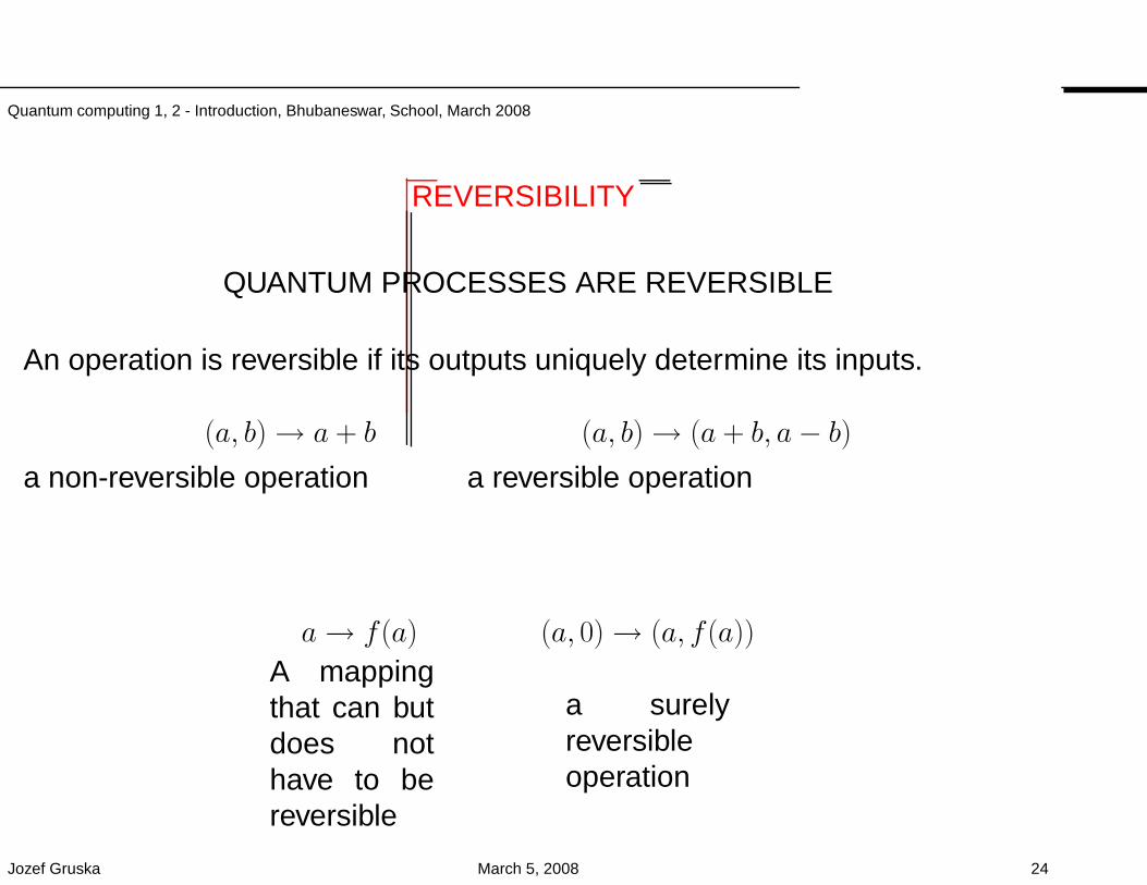
REVERSIBILITY
QUANTUM PROCESSES ARE REVERSIBLE
An operation is reversible if its outputs uniquely determine its inputs.
(a, b)→ a + b (a, b)→ (a + b, a− b)a non-reversible operation a reversible operation
a→ f(a) (a, 0)→ (a, f(a))
A mappingthat can butdoes nothave to bereversible
a surelyreversibleoperation
Jozef Gruska March 5, 2008 24
Quantum computing 1, 2 - Introduction, Bhubaneswar, School, March 2008
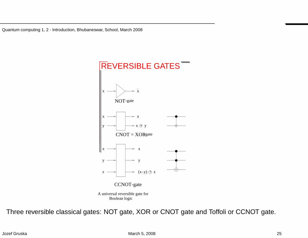
REVERSIBLE GATES
x x
x x
y x + y
x
y
z
x
y
(x y) + z
NOT
CNOT = XOR
-gate
-gate
CCNOT-gate
A universal reversible gate forBoolean logic
Three reversible classical gates: NOT gate, XOR or CNOT gate and Toffoli or CCNOT gate.
Jozef Gruska March 5, 2008 25
Quantum computing 1, 2 - Introduction, Bhubaneswar, School, March 2008
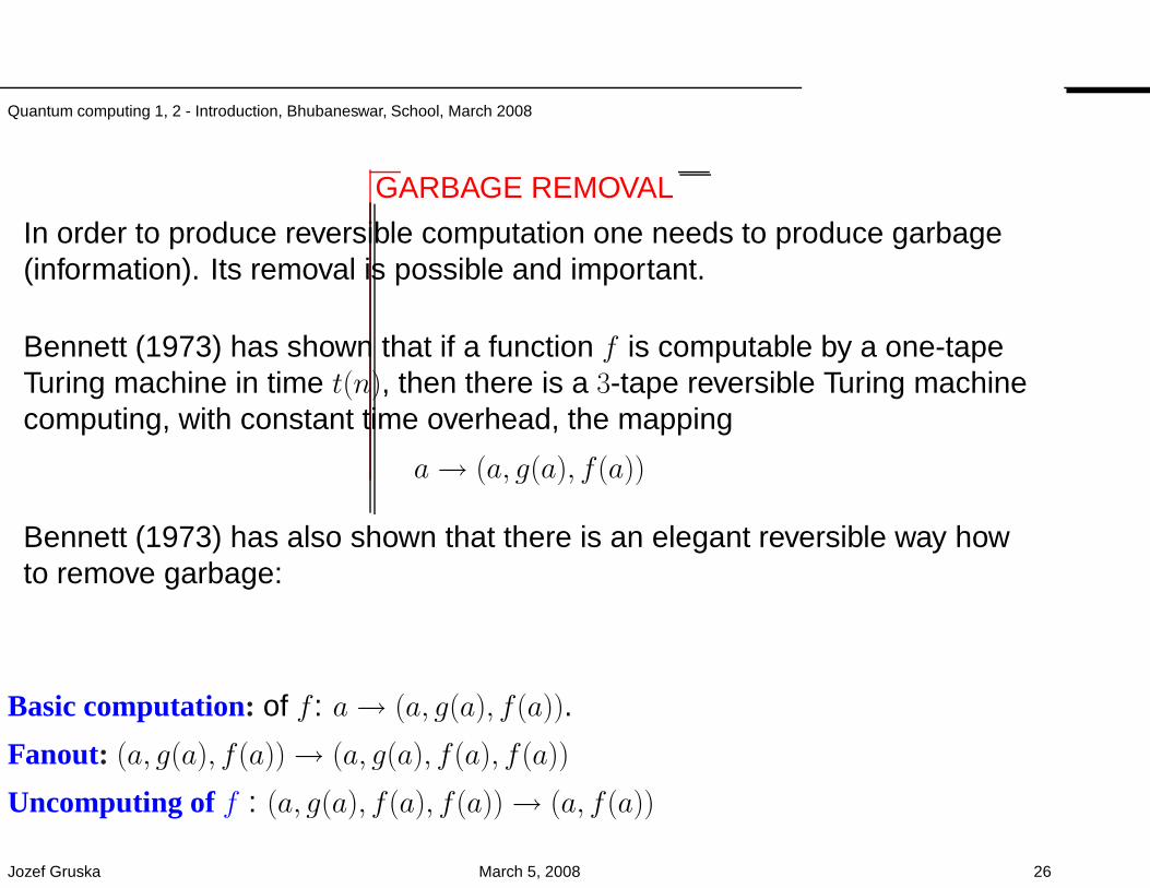
GARBAGE REMOVAL
In order to produce reversible computation one needs to produce garbage(information). Its removal is possible and important.
Bennett (1973) has shown that if a function f is computable by a one-tapeTuring machine in time t(n), then there is a 3-tape reversible Turing machinecomputing, with constant time overhead, the mapping
a→ (a, g(a), f(a))
Bennett (1973) has also shown that there is an elegant reversible way howto remove garbage:
Basic computation: of f : a→ (a, g(a), f(a)).
Fanout: (a, g(a), f(a))→ (a, g(a), f(a), f(a))
Uncomputing of f : (a, g(a), f(a), f(a))→ (a, f(a))
Jozef Gruska March 5, 2008 26
Quantum computing 1, 2 - Introduction, Bhubaneswar, School, March 2008
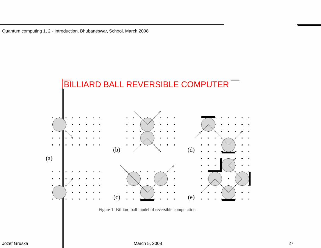
BILLIARD BALL REVERSIBLE COMPUTER
. .(a)
(b)
(c) (e)
(d)
Figure 1: Billiard ball model of reversible computation
Jozef Gruska March 5, 2008 27
Quantum computing 1, 2 - Introduction, Bhubaneswar, School, March 2008
c
x
c
c x
x
c xc = 0
x
c xc = 1
_c x c x c x
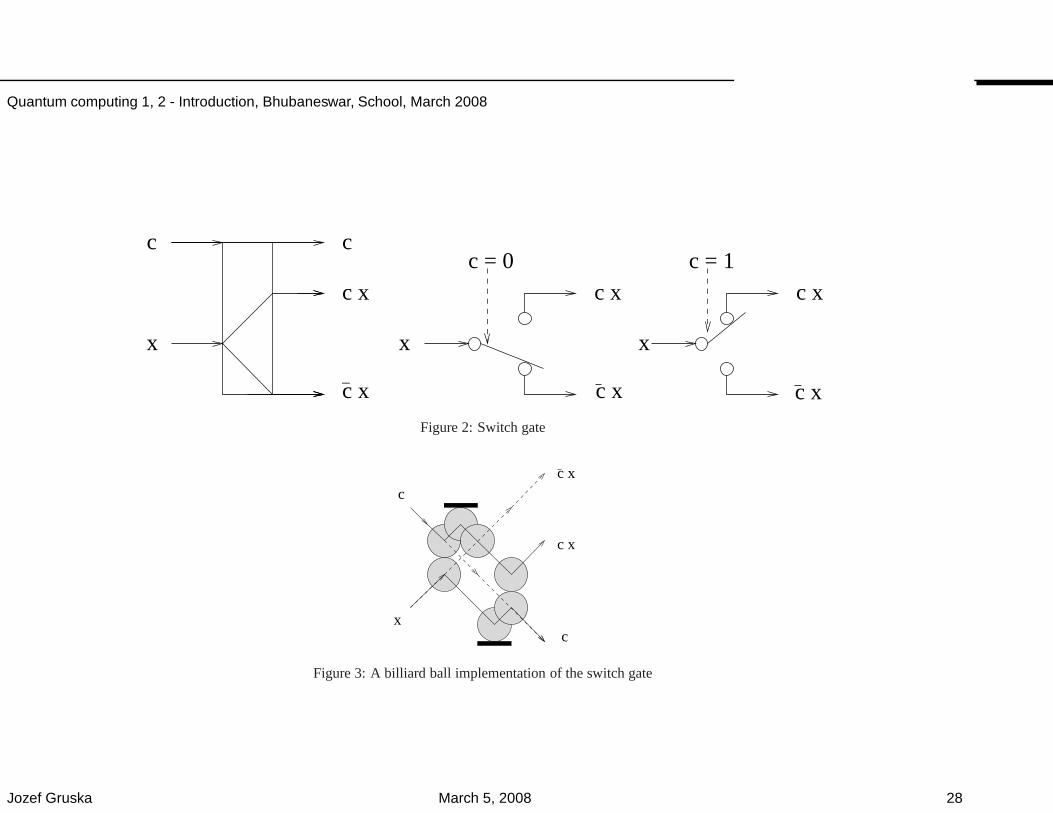
Figure 2: Switch gate
c
x
c x
c
c x
Figure 3: A billiard ball implementation of the switch gate
Jozef Gruska March 5, 2008 28
Quantum computing 1, 2 - Introduction, Bhubaneswar, School, March 2008
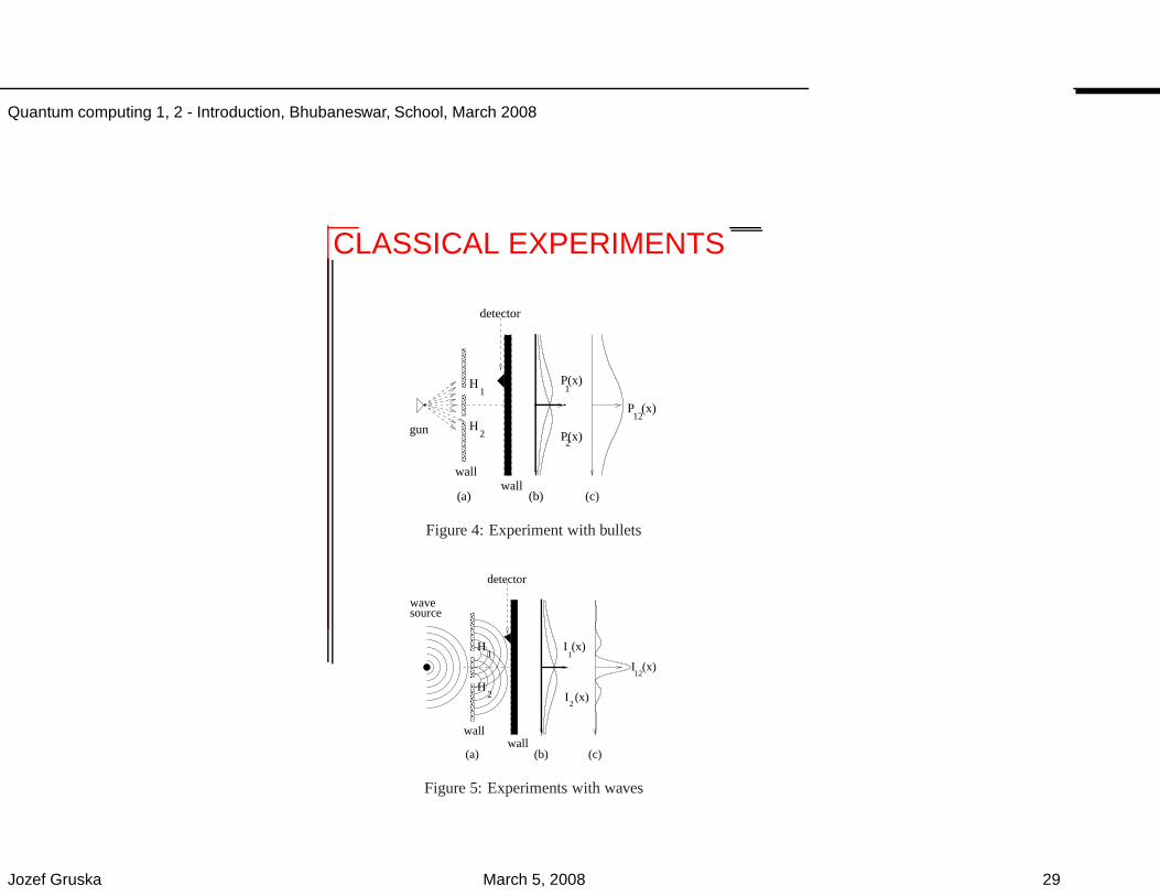
CLASSICAL EXPERIMENTS
gun
wall
detector
P
P
1
2
12
H
H
(c)
2
1P(x)
(x)
(x)
wall(b)(a)
Figure 4: Experiment with bullets
source
wall
detector
2
H
H
(a) (b) (c)
2
wave
I
I (x)
(x)
(x)
1
wall
I12
1
Figure 5: Experiments with waves
Jozef Gruska March 5, 2008 29
Quantum computing 1, 2 - Introduction, Bhubaneswar, School, March 2008
gun
wall
detector
P
P
1
2
12
H
H
(c)
2
1P(x)
(x)
(x)
wall(b)(a)
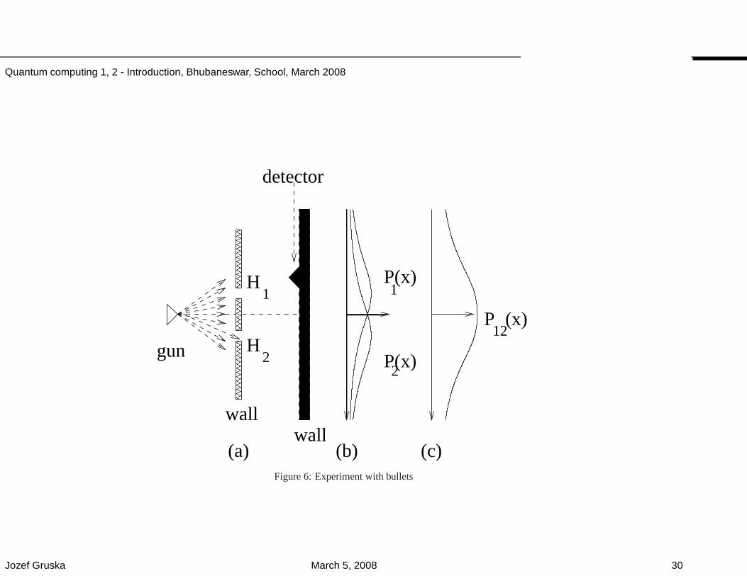
Figure 6: Experiment with bullets
Jozef Gruska March 5, 2008 30
Quantum computing 1, 2 - Introduction, Bhubaneswar, School, March 2008
source
wall
detector
2
H
H
(a) (b) (c)
2
wave
I
I (x)
(x)
(x)
1
wall
I12
1
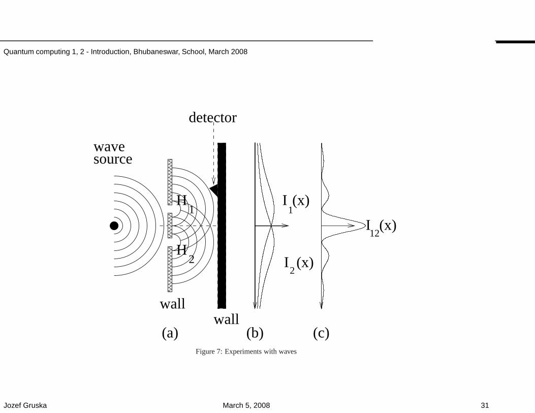
Figure 7: Experiments with waves
Jozef Gruska March 5, 2008 31
Quantum computing 1, 2 - Introduction, Bhubaneswar, School, March 2008
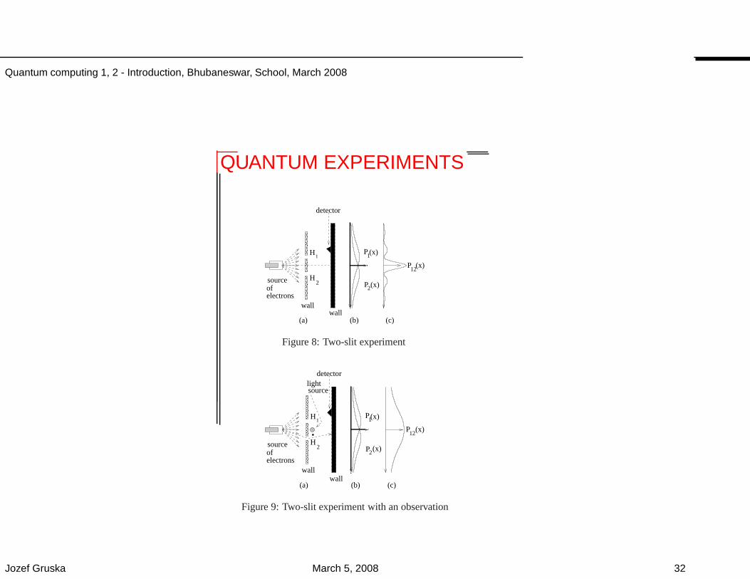
QUANTUM EXPERIMENTS
(x)
12P
wall
detector
1
2
H
(a) (b) (c)
2H
1
sourceofelectrons
P
P
(x)
(x)
wall
Figure 8: Two-slit experiment
wall
detector
1
2
H
(a) (b) (c)
2
12
H
1
sourceofelectrons
P
P
P
lightsource
(x)
(x)
(x)
wall
Figure 9: Two-slit experiment with an observation
Jozef Gruska March 5, 2008 32
Quantum computing 1, 2 - Introduction, Bhubaneswar, School, March 2008
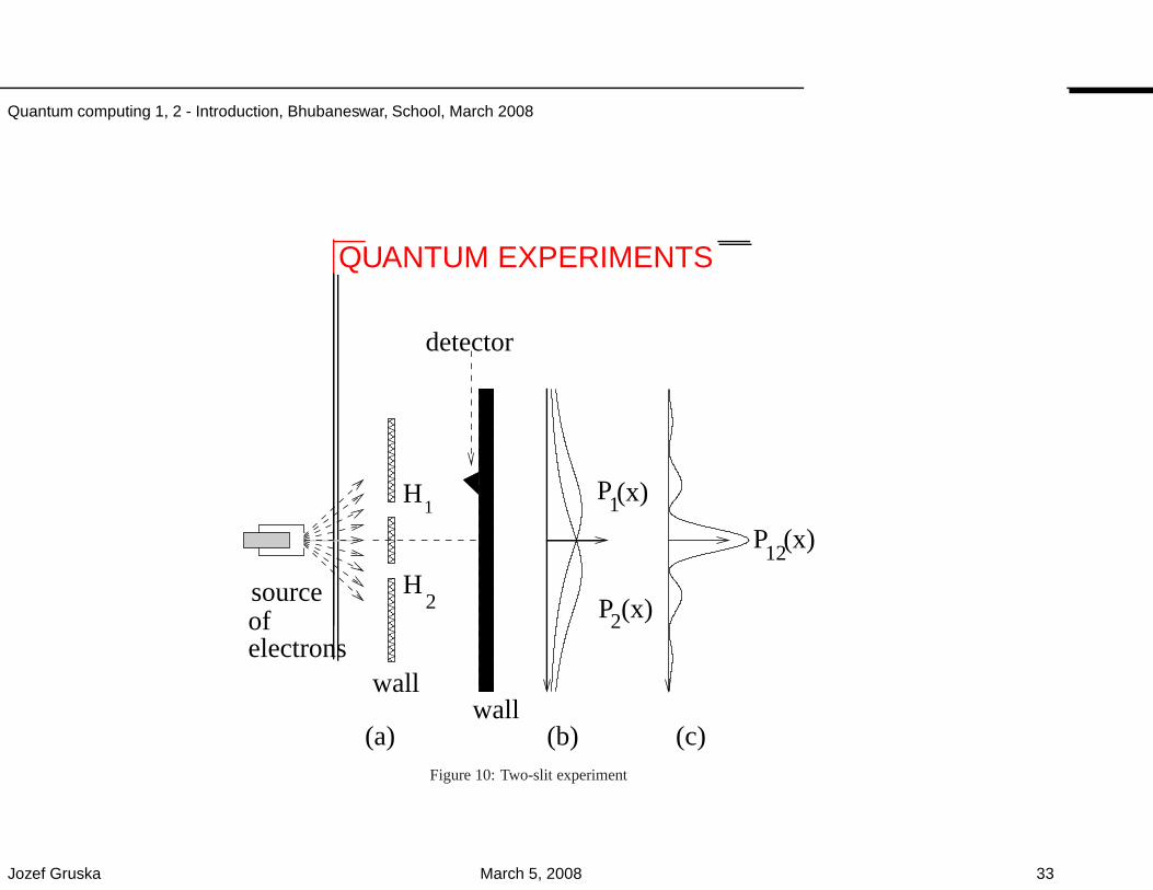
QUANTUM EXPERIMENTS
(x)
12P
wall
detector
1
2
H
(a) (b) (c)
2H
1
sourceofelectrons
P
P
(x)
(x)
wall
Figure 10: Two-slit experiment
Jozef Gruska March 5, 2008 33
Quantum computing 1, 2 - Introduction, Bhubaneswar, School, March 2008
wall
detector
1
2
H
(a) (b) (c)
2
12
H
1
sourceofelectrons
P
P
P
lightsource
(x)
(x)
(x)
wall
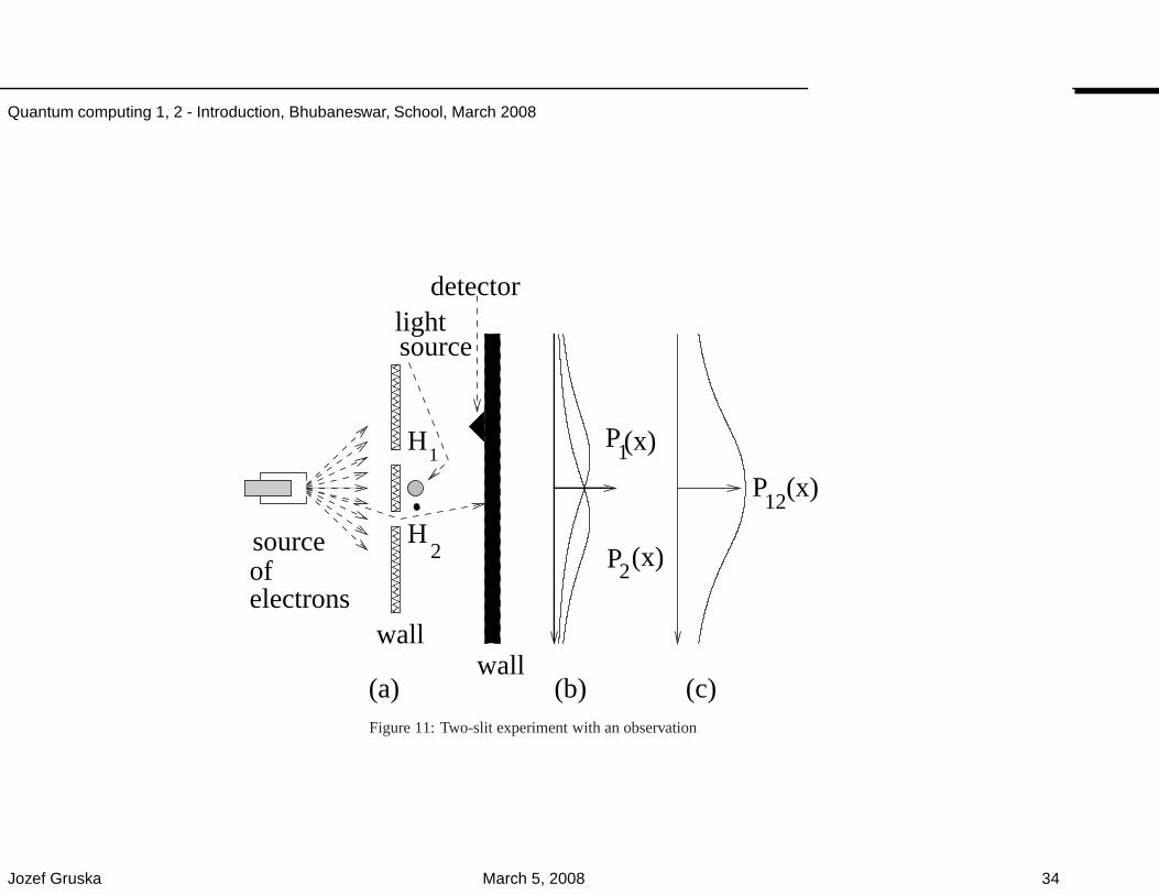
Figure 11: Two-slit experiment with an observation
Jozef Gruska March 5, 2008 34
Quantum computing 1, 2 - Introduction, Bhubaneswar, School, March 2008
TWO-SLIT EXPERIMENT – OBSERVATIONS
• Contrary to our intuition, at some places one observes fewerelectrons when both slits are open, than in the case only oneslit is open.
• Electrons — particles, seem to behave as waves.
• Each electron seems to behave as going through both holesat once.
• Results of the experiment do not depend on frequency withwhich electrons are shot.
•Quantum physics has no explanation where a particularelectron reaches the detector wall. All quantum physics canoffer are statements on the probability that an electronreaches a certain position on the detector wall.
Jozef Gruska March 5, 2008 35
Quantum computing 1, 2 - Introduction, Bhubaneswar, School, March 2008
BOHR’s WAVE-PARTICLE DUALITY PRINCIPLES
• Things we consider as waves correspond actually to particlesand things we consider as particles have waves associatedwith them.
• The wave is associated with the position of a particle - theparticle is more likely to be found in places where its wave isbig.
• The distance between the peaks of the wave is related to theparticle’s speed; the smaller the distance, the faster particlemoves.
• The wave’s frequency is proportional to the particle’s energy.(In fact, the particle’s energy i s equal exactly to its frequencytimes Planck’s constant.)
Jozef Gruska March 5, 2008 36
Quantum computing 1, 2 - Introduction, Bhubaneswar, School, March 2008
QUANTUM MECHANICS
•Quantum mechanicsis a theory that describes atomic andsubatomic particles and their interactions.
•Quantum mechanics was born around 1925.
• A physical system consisting of one or more quantum particles iscalled aquantum system.
• To completely describe a quantum particle aninfinite-dimensional Hilbert spaceis needed.
• For quantum computational purposes it is sufficient a partialdescription of particle(s) given in afinite-dimensional Hilbert(inner-product) space.
• To each isolated quantum system we associate an inner-productvector space elements of which of norm 1 are called(pure) states.
Jozef Gruska March 5, 2008 37
Quantum computing 1, 2 - Introduction, Bhubaneswar, School, March 2008
THREE BASIC PRINCIPLES
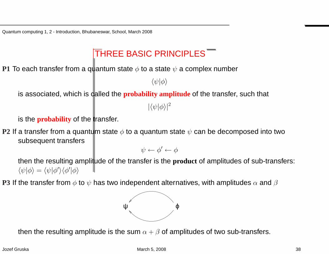
P1 To each transfer from a quantum state φ to a state ψ a complex number
〈ψ|φ〉is associated, which is called the probability amplitude of the transfer, such that
|〈ψ|φ〉|2
is the probability of the transfer.
P2 If a transfer from a quantum state φ to a quantum state ψ can be decomposed into twosubsequent transfers
ψ ← φ′ ← φ
then the resulting amplitude of the transfer is the product of amplitudes of sub-transfers:〈ψ|φ〉 = 〈ψ|φ′〉〈φ′|φ〉
P3 If the transfer from φ to ψ has two independent alternatives, with amplitudes α and β
ϕψ
then the resulting amplitude is the sum α + β of amplitudes of two sub-transfers.
Jozef Gruska March 5, 2008 38
Quantum computing 1, 2 - Introduction, Bhubaneswar, School, March 2008
QUANTUM SYSTEM = HILBERT SPACE
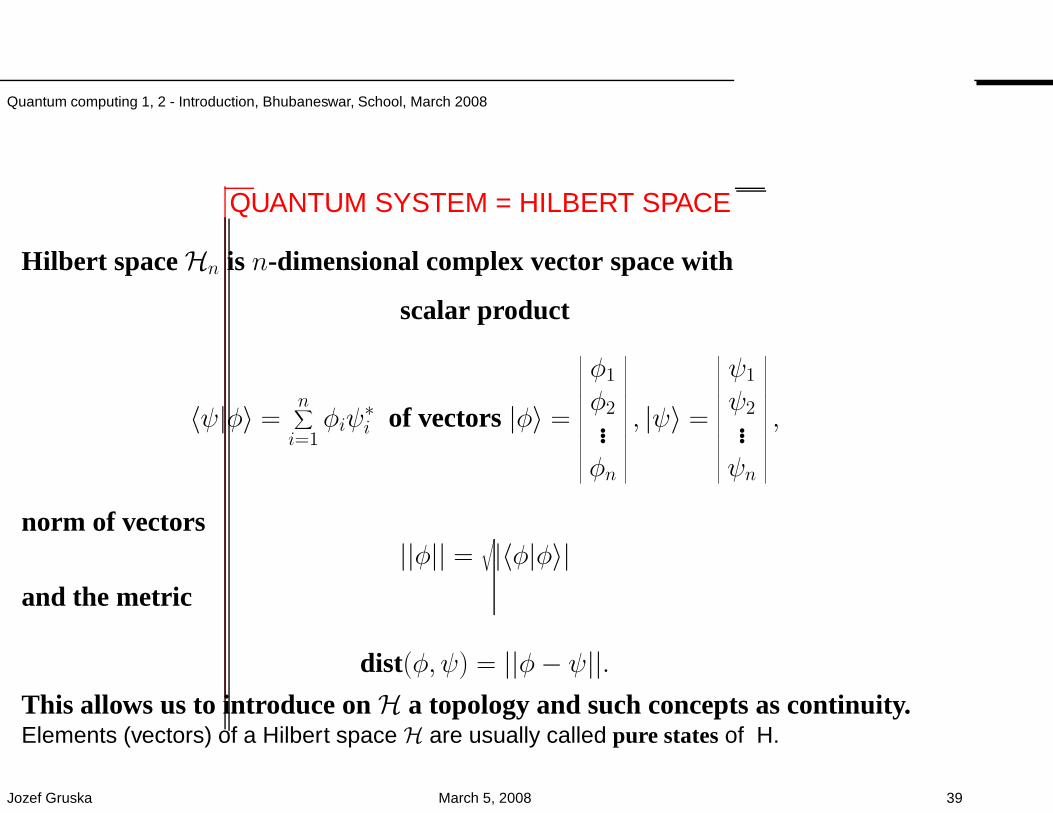
Hilbert spaceHn is n-dimensional complex vector space with
scalar product
〈ψ|φ〉 =n∑
i=1φiψ
∗i of vectors |φ〉 =
∣
∣
∣
∣
∣
∣
∣
∣
∣
∣
∣
∣
∣
∣
∣
∣
φ1
φ2...φn
∣
∣
∣
∣
∣
∣
∣
∣
∣
∣
∣
∣
∣
∣
∣
∣
, |ψ〉 =
∣
∣
∣
∣
∣
∣
∣
∣
∣
∣
∣
∣
∣
∣
∣
∣
ψ1
ψ2...ψn
∣
∣
∣
∣
∣
∣
∣
∣
∣
∣
∣
∣
∣
∣
∣
∣
,
norm of vectors||φ|| =
√
|〈φ|φ〉|and the metric
dist(φ, ψ) = ||φ− ψ||.This allows us to introduce onH a topology and such concepts as continuity.Elements (vectors) of a Hilbert space H are usually called pure statesof H.
Jozef Gruska March 5, 2008 39
Quantum computing 1, 2 - Introduction, Bhubaneswar, School, March 2008
ORTHOGONALITY of PURE STATES
Two quantum states|φ〉 and |ψ〉 are calledorthogonal if theirscalar product is zero, that is if
〈φ|ψ〉 = 0.
Two pure quantum states are physically perfectly distinguishableonly if they are orthogonal.In every Hilbert space there are so-calledorthogonal basesallstates of which are mutually orthogonal.
Jozef Gruska March 5, 2008 40
Quantum computing 1, 2 - Introduction, Bhubaneswar, School, March 2008
BRA-KET NOTATION
Dirac introduced a very handy notation, so called bra-ket notation, to dealwith amplitudes, quantum states and linear functionals f : H → C.
If ψ, φ ∈ H, then
〈ψ|φ〉— a number - a scalar product of ψ and φ(an amplitude of going from φ to ψ).
|φ〉— ket-vector — a column vector - an equivalent to φ
〈ψ|— bra-vector – a row vector - the conjugate transpose of |ψ〉 – a linearfunctional on H
such that 〈ψ|(|φ〉) = 〈ψ|φ〉Jozef Gruska March 5, 2008 41
Quantum computing 1, 2 - Introduction, Bhubaneswar, School, March 2008
Example If φ = (φ1, . . . , φn) and ψ = (ψ1, . . . , ψn), then
ket vector - |φ〉 =
φ1...φn
and 〈ψ| = (ψ∗1, . . . , ψ∗n) − bra-vector
andinner product - scalar product: 〈φ|ψ〉 =
n∑
i=1φ∗iψi
outer product: |φ〉〈ψ| =
φ1ψ∗1 . . . φ1ψ
∗n... . . . ...
φnψ∗1
... φnψ∗n
It is often said that physical counterparts of vectors of n-dimensional Hilbertspaces are n-level quantum systems.
Jozef Gruska March 5, 2008 42
Quantum computing 1, 2 - Introduction, Bhubaneswar, School, March 2008
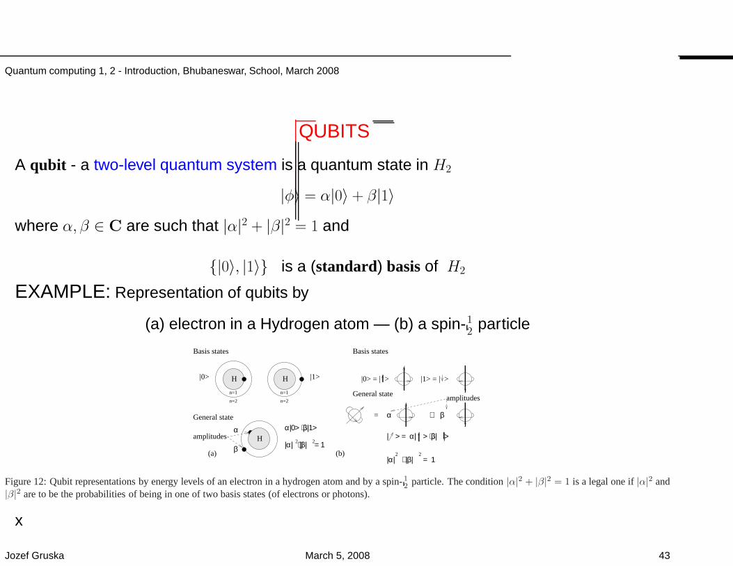
QUBITS
A qubit - a two-level quantum system is a quantum state in H2
|φ〉 = α|0〉 + β|1〉
where α, β ∈ C are such that |α|2 + |β|2 = 1 and
|0〉, |1〉 is a (standard) basisof H2
EXAMPLE: Representation of qubits by
(a) electron in a Hydrogen atom — (b) a spin-12
particle
n=1
Basis states
|0> |1>H H
Hamplitudes
(a) (b)
|0> = | > |1> = |
General state
=
amplitudes
α
β
α|0> + β|1>
|α| + |β| = 1
α + β
| > = α| > + β| >
|α| + |β| = 1
2
2 2
>
General state
2
n=1
n=2n=2
Basis states
Figure 12: Qubit representations by energy levels of an electron in a hydrogen atom and by a spin-1
2particle. The condition|α|2 + |β|2 = 1 is a legal one if|α|2 and
|β|2 are to be the probabilities of being in one of two basis states(of electrons or photons).
x
Jozef Gruska March 5, 2008 43
Quantum computing 1, 2 - Introduction, Bhubaneswar, School, March 2008
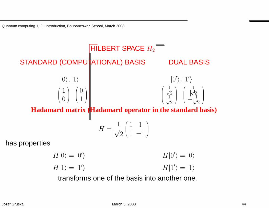
HILBERT SPACE H2
STANDARD (COMPUTATIONAL) BASIS DUAL BASIS
|0〉, |1〉 |0′〉, |1′〉
10
01
1√2
1√2
1√2
− 1√2
Hadamard matrix (Hadamard operator in the standard basis)
H =1√2
1 11 −1
has properties
H|0〉 = |0′〉 H|0′〉 = |0〉H|1〉 = |1′〉 H|1′〉 = |1〉
transforms one of the basis into another one.
Jozef Gruska March 5, 2008 44
Quantum computing 1, 2 - Introduction, Bhubaneswar, School, March 2008
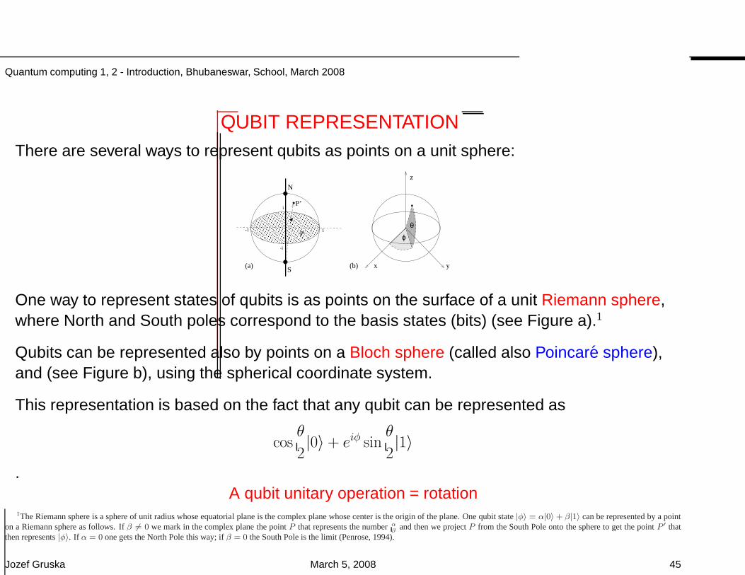
QUBIT REPRESENTATIONThere are several ways to represent qubits as points on a unit sphere:
-1 1
-i
i
N
S
P
x
z
(a) (b) y
P’
θ
ϕ
One way to represent states of qubits is as points on the surface of a unit Riemann sphere,where North and South poles correspond to the basis states (bits) (see Figure a).1
Qubits can be represented also by points on a Bloch sphere (called also Poincare sphere),and (see Figure b), using the spherical coordinate system.
This representation is based on the fact that any qubit can be represented as
cosθ
2|0〉 + eiφ sin
θ
2|1〉
.A qubit unitary operation = rotation
1The Riemann sphere is a sphere of unit radius whose equatorial plane is the complex plane whose center is the origin of the plane. One qubit state|φ〉 = α|0〉 + β|1〉 can be represented by a pointon a Riemann sphere as follows. Ifβ 6= 0 we mark in the complex plane the pointP that represents the numberα
βand then we projectP from the South Pole onto the sphere to get the pointP ′ that
then represents|φ〉. If α = 0 one gets the North Pole this way; ifβ = 0 the South Pole is the limit (Penrose, 1994).
Jozef Gruska March 5, 2008 45
Quantum computing 1, 2 - Introduction, Bhubaneswar, School, March 2008
REALISATION of ROTATION on SPIN-1/2 PARTICLES
• For states of standard and dual basis of spin-1/2 particles one often uses the followingnotation:
|0〉 = | ↑〉, |1〉 = | ↓〉, | →〉 =1√2(|0〉 + |1〉), | ←〉 =
1√2(|0〉 − |1〉)
• If such a particle is put into a magnetic field it starts (its spin-orientation) to rotate. Let tbe time for a full rotation.
• After rotation time t/4 the particle will be in the state
| →〉 =1√2(|0〉 + |1〉);
• After rotation time t/2 the particle will be in the state
|1〉 = | ↓〉.
• After rotation time 3t/4 the particle will be in the state
| ←〉 =1√2(|0〉 − |1〉)
;
• In all other times the particle will be in all other potential superpositions of two basisstates.
Jozef Gruska March 5, 2008 46
Quantum computing 1, 2 - Introduction, Bhubaneswar, School, March 2008
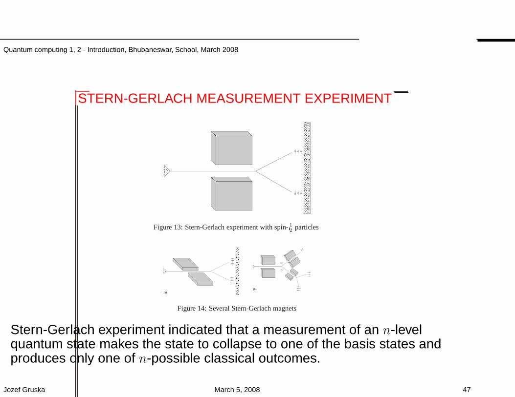
STERN-GERLACH MEASUREMENT EXPERIMENT
Figure 13: Stern-Gerlach experiment with spin-1
2particles
(a)(b)
Figure 14: Several Stern-Gerlach magnets
Stern-Gerlach experiment indicated that a measurement of an n-levelquantum state makes the state to collapse to one of the basis states andproduces only one of n-possible classical outcomes.
Jozef Gruska March 5, 2008 47
Quantum computing 1, 2 - Introduction, Bhubaneswar, School, March 2008
QUANTUM (PROJECTION) MEASUREMENTS
A quantum state is observed (measured) with respect to an observable— a decompositionof a given Hilbert space into orthogonal subspaces (such that each vector can be uniquelyrepresented as a sum of vectors of these subspaces).
There are two outcomes of a projection measurement of a state |φ〉:1. Classical information into which subspace projection of |φ〉 was made.
2. A new quantum state |φ′〉 into which the state |φ〉 collapses.
The subspace into which projection is made is chosen randomly and the correspondingprobability is uniquely determined by the amplitudes at the representation of |φ〉 at the basisstates of the subspace.
Jozef Gruska March 5, 2008 48
Quantum computing 1, 2 - Introduction, Bhubaneswar, School, March 2008
QUANTUM STATES and PROJECTION MEASUREMENT
In case an orthonormal basis βini=1 is chosen in Hn, any state|φ〉 ∈ Hn can be expressed in the form
|φ〉 =n∑
i=1ai|βi〉,
n∑
i=1|ai|2 = 1,
whereai = 〈βi|φ〉 are called probability amplitudes
andtheir squares, |ai|2, provide probabilities
that if the state |φ〉 is measured with respect to the basisβini=1, then the state |φ〉 collapses into the state |βi〉 withprobability |ai|2.The classical “outcome” of a measurement of the state |φ〉 withrespect to the basis βini=1 is the index i of that state |βi〉 intowhich the state |φ〉 collapses.
Jozef Gruska March 5, 2008 49
Quantum computing 1, 2 - Introduction, Bhubaneswar, School, March 2008
PHYSICAL VIEW of QUANTUM MEASUREMENT
In case an orthonormal basisβini=1 is chosen inHn, it is saidthat an observablewas chosen.
In such a case, ameasurement, or an observation, of a state
|φ〉 =n∑
i=1ai|βi〉,
n∑
i=1|ai|2 = 1,
with respect to a basis (observable),βini=1, is seen as saying thatthe state|φ〉 hasproperty |βi〉 with probability |ai|2.In general, any decomposition of a Hilbert spaceH into mutuallyorthogonal subspaces, with the property that any quantum statecan be uniquely expressed as the sum of the states from suchsubspaces, represents an observable (a measuring device).Thereare no other observables.
Jozef Gruska March 5, 2008 50
Quantum computing 1, 2 - Introduction, Bhubaneswar, School, March 2008
WHAT ARE ACTUALLY QUANTUM STATES? - TWO VIEWS
• In so called “relative state interpretation” of quantummechanics a quantum state is interpreted as an objective realphysical object.
• In so called “information view of quantum mechanics” aquantum state is interpreted as a specification of (ourknowledge or beliefs) probabilities of all experiments that canbe performed with the state - the idea that quantum statesdescribe the reality is therefore abounded.
A quantum state is a useful abstraction which frequently appears in the literature, but doesnot really exists in nature.
A. Peres (1993)
Jozef Gruska March 5, 2008 51
Quantum computing 1, 2 - Introduction, Bhubaneswar, School, March 2008
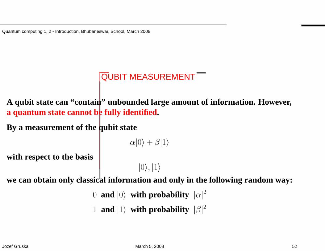
QUBIT MEASUREMENT
A qubit state can “contain” unbounded large amount of information. However,a quantum state cannot be fully identified.
By a measurement of the qubit state
α|0〉 + β|1〉with respect to the basis
|0〉, |1〉we can obtain only classical information and only in the following random way:
0 and |0〉 with probability |α|2
1 and |1〉 with probability |β|2
Jozef Gruska March 5, 2008 52
Quantum computing 1, 2 - Introduction, Bhubaneswar, School, March 2008
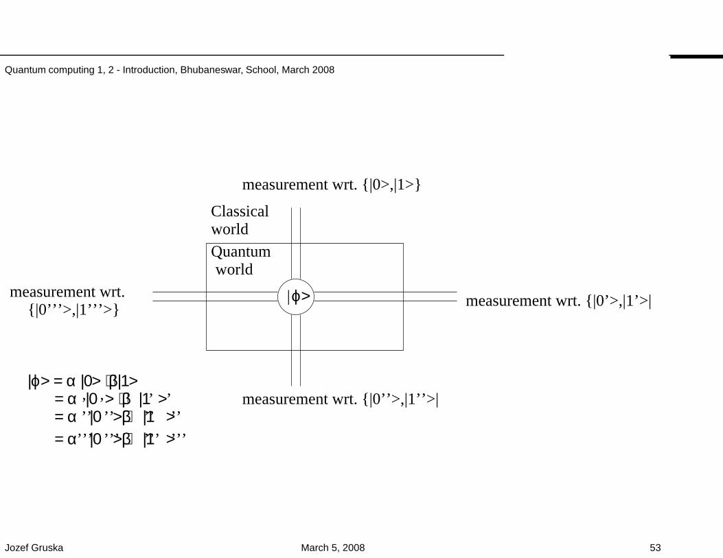
Quantumworld
Classicalworld
|0’’’>,|1’’’>|ϕ>
|ϕ> = α |0> + β|1>= α |0 > + β |1 >= α |0 >+β |1 >= α |0 >+β |1 >
’ ’ ’ ’’’ ’’ ’’ ’’’’’ ’’’ ’’’ ’’’
measurement wrt. |0>,|1>
measurement wrt. |0’>,|1’>|measurement wrt.
measurement wrt. |0’’>,|1’’>|
Jozef Gruska March 5, 2008 53
Quantum computing 1, 2 - Introduction, Bhubaneswar, School, March 2008
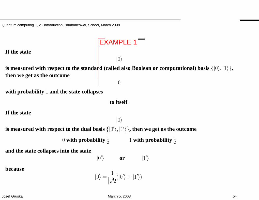
EXAMPLE 1If the state
|0〉is measured with respect to the standard (called also Boolean or computational) basis|0〉, |1〉,then we get as the outcome
0
with probability 1 and the state collapses
to itself.
If the state|0〉
is measured with respect to the dual basis|0′〉, |1′〉, then we get as the outcome
0 with probability 12 1 with probability 1
2
and the state collapses into the state|0′〉 or |1′〉
because|0〉 =
1√2(|0′〉 + |1′〉).
Jozef Gruska March 5, 2008 54
Quantum computing 1, 2 - Introduction, Bhubaneswar, School, March 2008
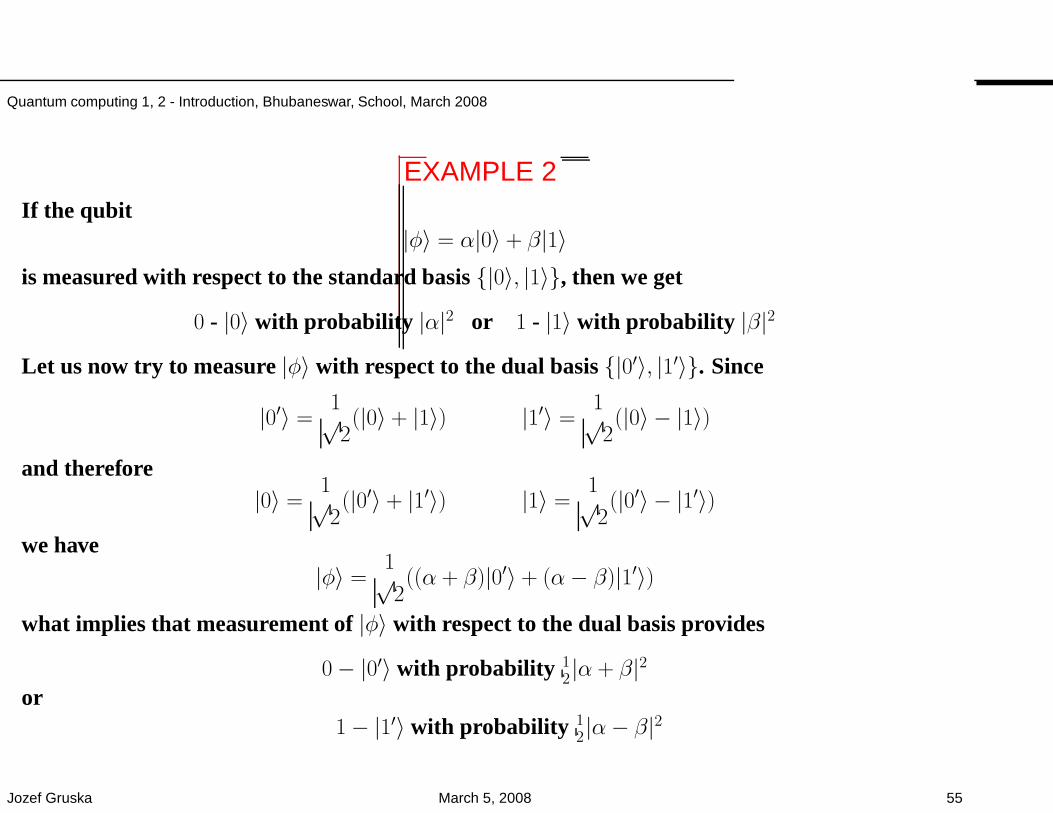
EXAMPLE 2If the qubit
|φ〉 = α|0〉 + β|1〉is measured with respect to the standard basis|0〉, |1〉, then we get
0 - |0〉 with probability |α|2 or 1 - |1〉 with probability |β|2
Let us now try to measure|φ〉 with respect to the dual basis|0′〉, |1′〉. Since
|0′〉 =1√2(|0〉 + |1〉) |1′〉 =
1√2(|0〉 − |1〉)
and therefore|0〉 =
1√2(|0′〉 + |1′〉) |1〉 =
1√2(|0′〉 − |1′〉)
we have|φ〉 =
1√2((α + β)|0′〉 + (α− β)|1′〉)
what implies that measurement of|φ〉 with respect to the dual basis provides
0− |0′〉 with probability 12|α + β|2
or1− |1′〉 with probability 1
2|α− β|2
Jozef Gruska March 5, 2008 55
Quantum computing 1, 2 - Introduction, Bhubaneswar, School, March 2008
HEISSENBERG’s UNCERTAINTY PRINCIPLE
• Heissenberg’s uncertainty principle says that if the value of a physicalquantity is certain, then the value of a complementary quality is uncertain.
• Example. Measurement with respect to standard basis of states |0〉 and |1〉gives certain outcome and therefore measurement of the same statesaccording to the dual basis provides uncertain (random) outcomes.
• Another pair of complementary quantities are position and speed.
Jozef Gruska March 5, 2008 56
Quantum computing 1, 2 - Introduction, Bhubaneswar, School, March 2008
WHAT ARE QUANTUM STATES?
• In the classical world we see a state as consisting of allinformation needed to describe completely the system at aninstant of time.
• Due to Heissenberg’s principle of uncertainty, such anapproach is not possible in quantum world - for example, wecannot describe exactly both position and velocity(momentum).
Jozef Gruska March 5, 2008 57
Quantum computing 1, 2 - Introduction, Bhubaneswar, School, March 2008
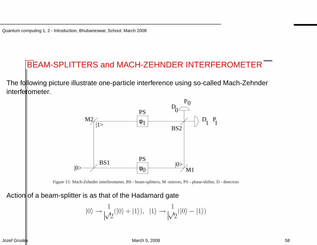
BEAM-SPLITTERS and MACH-ZEHNDER INTERFEROMETER
The following picture illustrate one-particle interference using so-called Mach-Zehnderinterferometer.
D
D
BS10
PS
M1
M2
BS2
PS
φ
φ1
|0>|0>
|1>
0
1
P
P
0
1
Figure 15: Mach-Zehnder interferometer, BS - beam-splitters, M -mirrors, PS - phase-shifter, D - detectors
Action of a beam-splitter is as that of the Hadamard gate
|0〉 → 1√2(|0〉 + |1〉), |1〉 → 1√
2(|0〉 − |1〉)
Jozef Gruska March 5, 2008 58
Quantum computing 1, 2 - Introduction, Bhubaneswar, School, March 2008
D
D
BS10
PS
M1
M2
BS2
PS
φ
φ1
|0>|0>
|1>
0
1
P
P
0
1
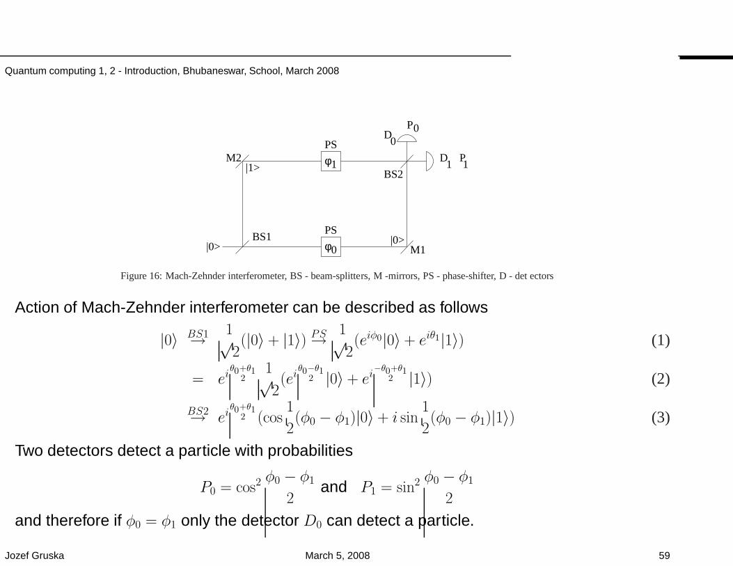
Figure 16: Mach-Zehnder interferometer, BS - beam-splitters, M -mirrors, PS - phase-shifter, D - det ectors
Action of Mach-Zehnder interferometer can be described as follows
|0〉 BS1→ 1√2(|0〉 + |1〉) PS→ 1√
2(eiφ0|0〉 + eiθ1|1〉) (1)
= eiθ0+θ1
21√2(ei
θ0−θ12 |0〉 + ei
−θ0+θ12 |1〉) (2)
BS2→ eiθ0+θ1
2 (cos1
2(φ0 − φ1)|0〉 + i sin
1
2(φ0 − φ1)|1〉) (3)
Two detectors detect a particle with probabilities
P0 = cos2 φ0 − φ1
2and P1 = sin2 φ0 − φ1
2
and therefore if φ0 = φ1 only the detector D0 can detect a particle.
Jozef Gruska March 5, 2008 59
Quantum computing 1, 2 - Introduction, Bhubaneswar, School, March 2008
OBSERVATION on INTERFERENCE EXPERIMENTS
• Single particle experiments are not restricted to photons.
•One can repeat such an experiment with electrons, atoms oreven some molecules.
•When it comes to atoms both internal and external degrees offreedom can be used
Jozef Gruska March 5, 2008 60
Quantum computing 1, 2 - Introduction, Bhubaneswar, School, March 2008
CLASSICAL versus QUANTUM COMPUTING
The essence of the differencebetween
classical computersand quantum computers
is in the way information is stored and processed.
In classical computers, information is represented on macroscopic levelbybits, which can take one of the two values
0 or 1
In quantum computers, information is represented on microscopic levelusingqubits, which can take on any from uncountable many values
α|0〉 + β|1〉where α, β are arbitrary complex numbers such that
|α|2 + |β|2 = 1.
Jozef Gruska March 5, 2008 61
Quantum computing 1, 2 - Introduction, Bhubaneswar, School, March 2008
QUANTUM EVOLUTION/COMPUTATIONEVOLUTION COMPUTATION
in in
QUANTUM SYSTEM HILBERT SPACE
is described by
Schrodinger linear equation
ih∂ψ(t)
∂t= H(t)ψ(t),
where H(t) is a quantum analogue of a Hamiltonian of the classical system, from which itfollows that ψ(t) = e−
ihH(t) and therefore that an discretized evolution (computation) step of a
quantum system is performed by a multiplication by a unitary operator and a step of suchan evolution we can see as a multiplication of a unitary matrix A with a vector |ψ〉, i.e.
A|ψ〉
A matrix A is unitary if for A and its adjoint matrix A† (with A†ij = (Aji)∗) it holds:
A · A† = A† · A = I
Jozef Gruska March 5, 2008 62
Quantum computing 1, 2 - Introduction, Bhubaneswar, School, March 2008
HAMILTONIANS
The Schrodinger equation tells us how a quantum system evolves
subject to the Hamiltonian
However, in order to do quantum mechanics, one has to knowhow to pick up the Hamiltonian.
The principles that tell us how to do so are real bridge principlesof quantum mechanics.Each quantum system is actually uniquely determined by aHamiltonian.
Jozef Gruska March 5, 2008 63
Quantum computing 1, 2 - Introduction, Bhubaneswar, School, March 2008
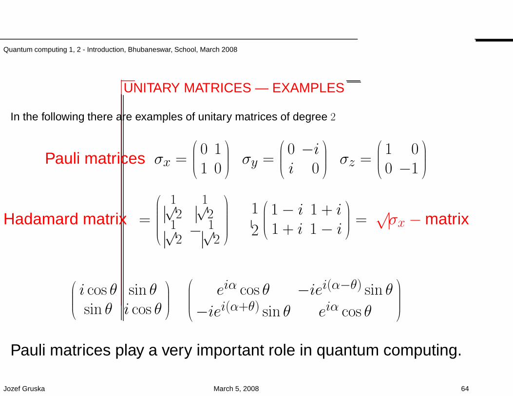
UNITARY MATRICES — EXAMPLES
In the following there are examples of unitary matrices of degree 2
Pauli matrices σx =
0 11 0
σy =
0 −ii 0
σz =
1 00 −1
Hadamard matrix =
1√2
1√2
1√2− 1√
2
1
2
1− i 1 + i1 + i 1− i
=√σx −matrix
i cos θ sin θsin θ i cos θ
eiα cos θ −iei(α−θ) sin θ
−iei(α+θ) sin θ eiα cos θ
Pauli matrices play a very important role in quantum computing.
Jozef Gruska March 5, 2008 64
Quantum computing 1, 2 - Introduction, Bhubaneswar, School, March 2008
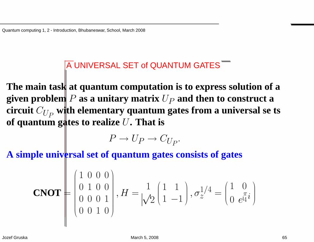
A UNIVERSAL SET of QUANTUM GATES
The main task at quantum computation is to express solution of agiven problemP as a unitary matrix UP and then to construct acircuit CUP with elementary quantum gates from a universal se tsof quantum gates to realizeU . That is
P → UP → CUP .
A simple universal set of quantum gates consists of gates
CNOT =
1 0 0 00 1 0 00 0 0 10 0 1 0
, H =1√2
1 11 −1
, σ1/4z =
1 0
0 eπ4 i
Jozef Gruska March 5, 2008 65
Quantum computing 1, 2 - Introduction, Bhubaneswar, School, March 2008
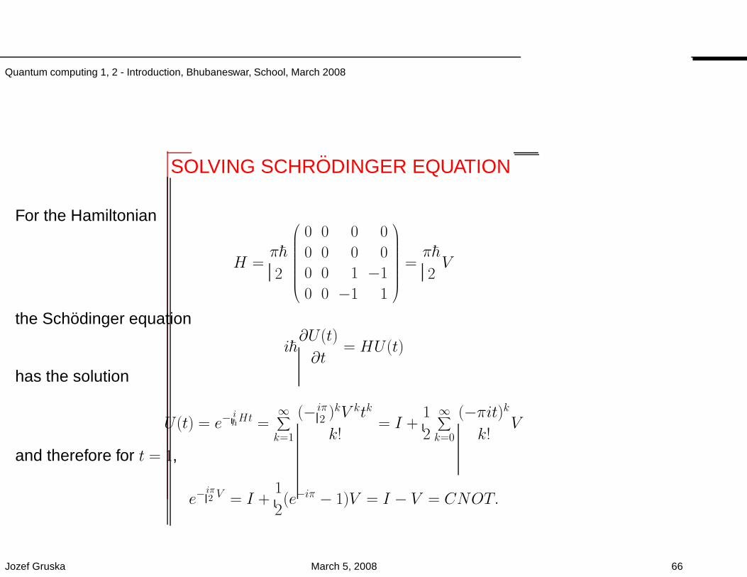
SOLVING SCHRODINGER EQUATION
For the Hamiltonian
H =πh
2
0 0 0 0
0 0 0 0
0 0 1 −1
0 0 −1 1
=πh
2V
the Schodinger equation
ih∂U(t)
∂t= HU(t)
has the solution
U(t) = e−ihHt =
∞∑
k=1
(− iπ2 )kV ktk
k!= I +
1
2
∞∑
k=0
(−πit)kk!
V
and therefore for t = 1,
e−iπ2 V = I +
1
2(e−iπ − 1)V = I − V = CNOT.
Jozef Gruska March 5, 2008 66
Quantum computing 1, 2 - Introduction, Bhubaneswar, School, March 2008
CLASSICAL versus QUANTUM MECHANICS
A crucial difference between quantum theory and classical mechanics isperhaps this: whereas classical states are essentially descriptive, quantumstates are essentially predictive; they encapsulate predictions concerningthe values that measurements of physical quantities will yield, and thesepredictions are in terms of probabilities.
The state of a classical particle is given by its position q = (qx, qy, qz) andmomentum p = (px, py, pz).
The state of n particles is therefore given by 6n numbers.
Hamiltonian, or total energy H(p, q) of a system of n particles is then afunction of 3n coordinates piu, i = 1, . . . ,, u ∈ x, y, z and 3n coordinates qiu.
Time evolution of such a system is then described by a system of 3n pairs ofHamiltonian equations
dqiudt
=∂H
∂piu
dpiudt
= −∂H∂qiu
Jozef Gruska March 5, 2008 67
Quantum computing 1, 2 - Introduction, Bhubaneswar, School, March 2008
MEASUREMENT
in CLASSICAL versus QUANTUM physics
BEFORE QUANTUM PHYSICS
it was taken for granted that when physicists measure something, they aregaining knowledge of a pre-existing state — a knowledge of an independentfact about the world.
QUANTUM PHYSICS
says otherwise. Things are not determined except when they are measured,and it is only by being measured that they take on specific values.
A quantum measurement forces a previously indeterminate system to takeon a definite value.
Jozef Gruska March 5, 2008 68
Quantum computing 1, 2 - Introduction, Bhubaneswar, School, March 2008
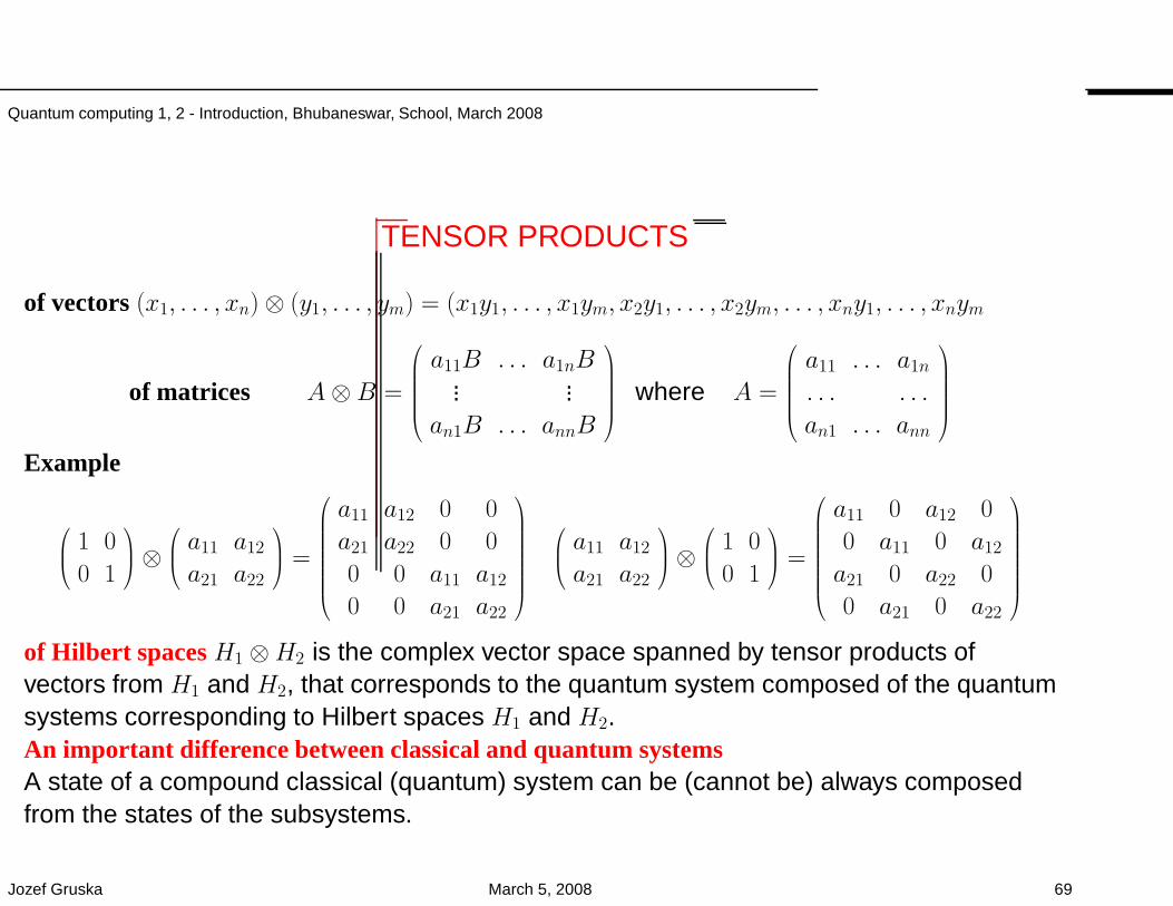
TENSOR PRODUCTS
of vectors(x1, . . . , xn)⊗ (y1, . . . , ym) = (x1y1, . . . , x1ym, x2y1, . . . , x2ym, . . . , xny1, . . . , xnym
of matrices A⊗ B =
a11B . . . a1nB... ...
an1B . . . annB
where A =
a11 . . . a1n
. . . . . .
an1 . . . ann
Example
1 0
0 1
⊗
a11 a12
a21 a22
=
a11 a12 0 0
a21 a22 0 0
0 0 a11 a12
0 0 a21 a22
a11 a12
a21 a22
⊗
1 0
0 1
=
a11 0 a12 0
0 a11 0 a12
a21 0 a22 0
0 a21 0 a22
of Hilbert spacesH1 ⊗H2 is the complex vector space spanned by tensor products ofvectors from H1 and H2, that corresponds to the quantum system composed of the quantumsystems corresponding to Hilbert spaces H1 and H2.An important difference between classical and quantum systemsA state of a compound classical (quantum) system can be (cannot be) always composedfrom the states of the subsystems.
Jozef Gruska March 5, 2008 69
Quantum computing 1, 2 - Introduction, Bhubaneswar, School, March 2008
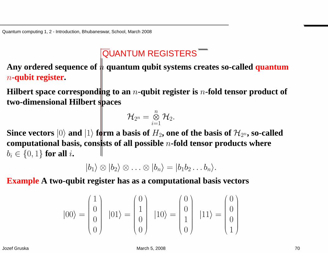
QUANTUM REGISTERS
Any ordered sequence ofn quantum qubit systems creates so-calledquantumn-qubit register.
Hilbert space corresponding to ann-qubit register is n-fold tensor product oftwo-dimensional Hilbert spaces
H2n =n
⊗
i=1H2.
Since vectors|0〉 and |1〉 form a basis ofH2, one of the basis ofH2n, so-calledcomputational basis, consists of all possiblen-fold tensor products wherebi ∈ 0, 1 for all i.
|b1〉 ⊗ |b2〉 ⊗ . . .⊗ |bn〉 = |b1b2 . . . bn〉.ExampleA two-qubit register has as a computational basis vectors
|00〉 =
1000
|01〉 =
0100
|10〉 =
0010
|11〉 =
0001
Jozef Gruska March 5, 2008 70
Quantum computing 1, 2 - Introduction, Bhubaneswar, School, March 2008
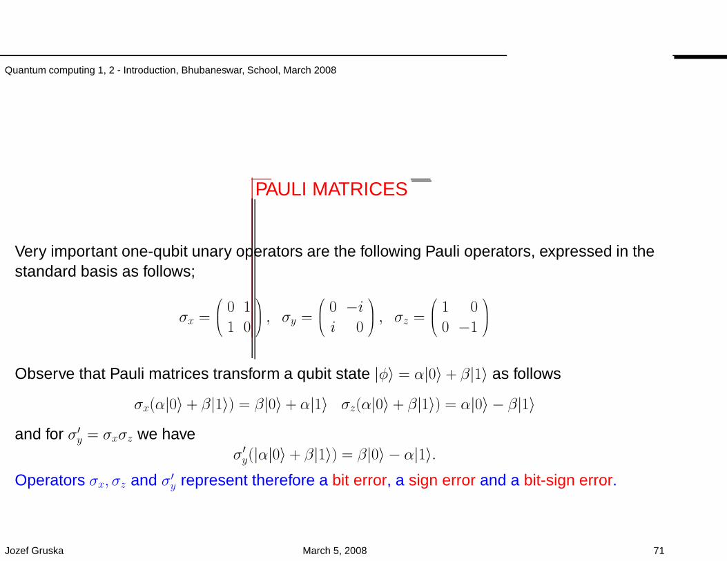
PAULI MATRICES
Very important one-qubit unary operators are the following Pauli operators, expressed in thestandard basis as follows;
σx =
0 1
1 0
, σy =
0 −ii 0
, σz =
1 0
0 −1
Observe that Pauli matrices transform a qubit state |φ〉 = α|0〉 + β|1〉 as follows
σx(α|0〉 + β|1〉) = β|0〉 + α|1〉 σz(α|0〉 + β|1〉) = α|0〉 − β|1〉
and for σ′y = σxσz we haveσ′y(|α|0〉 + β|1〉) = β|0〉 − α|1〉.
Operators σx, σz and σ′y represent therefore a bit error, a sign error and a bit-sign error.
Jozef Gruska March 5, 2008 71
Quantum computing 1, 2 - Introduction, Bhubaneswar, School, March 2008
MIXED STATES - DENSITY MATRICES
A probability distribution (pi, |φi〉ki=1 on pure states is called a mixed stateto which it is assigned a density operator
ρ =k∑
i=1pi|φi〉〈φi|.
One interpretation of a mixed state pi, |φi〉ki=1 is that a source X producesthe state |φi〉 with probability pi.
Any matrix representing a density operator is called density matrix.
To two different mixed states can correspond the same density matrix.
Two mixed states with the same density matrix are physicallyundistinguishable.
Jozef Gruska March 5, 2008 72
Quantum computing 1, 2 - Introduction, Bhubaneswar, School, March 2008
DENSITY MATRICES
Density matrices are exactly matrices that are Hermitian,positive and have trace 1.
Eigenvalues of a density matrix are real, nonnegative and sumup to one - density matrices can be seen as a generalisation ofprobability distributions.
For any pure state |φ〉, |φ〉〈φ| is a density matrix (representing|φ〉).Density matrices represent a class of similar mixed states andare also often called states.
Jozef Gruska March 5, 2008 73
Quantum computing 1, 2 - Introduction, Bhubaneswar, School, March 2008
MAXIMALLY MIXED STATES
To the maximally mixed state
(1
2, |0〉), (1
2, |1〉)
which represents a random bit corresponds the density matrix
1
2
10
(1, 0) +1
2
01
(0, 1) =1
2
1 00 1
=1
2I2
Surprisingly, many other mixed states have as their densitymatrix that one of the maximally mixed state.
Jozef Gruska March 5, 2008 74
Quantum computing 1, 2 - Introduction, Bhubaneswar, School, March 2008
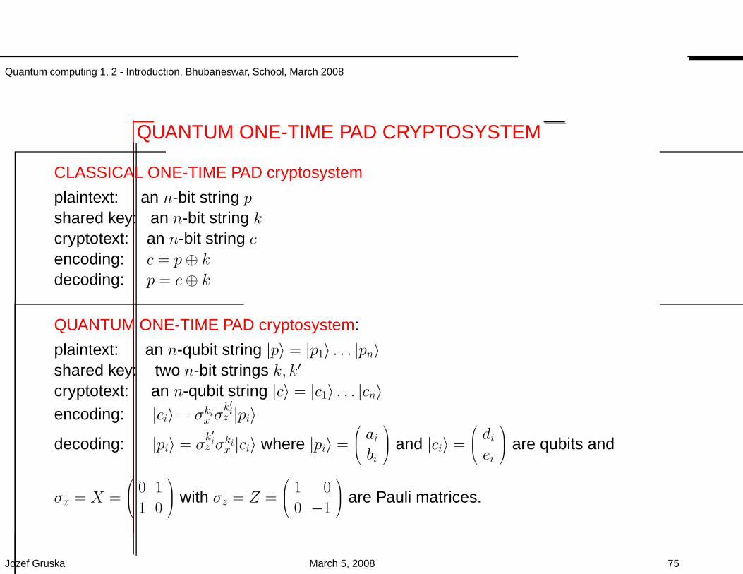
QUANTUM ONE-TIME PAD CRYPTOSYSTEM
CLASSICAL ONE-TIME PAD cryptosystem
plaintext: an n-bit string pshared key: an n-bit string kcryptotext: an n-bit string cencoding: c = p⊕ kdecoding: p = c⊕ k
QUANTUM ONE-TIME PAD cryptosystem:
plaintext: an n-qubit string |p〉 = |p1〉 . . . |pn〉shared key: two n-bit strings k, k′
cryptotext: an n-qubit string |c〉 = |c1〉 . . . |cn〉encoding: |ci〉 = σki
x σk′iz |pi〉
decoding: |pi〉 = σk′iz σki
x |ci〉 where |pi〉 =
aibi
and |ci〉 =
diei
are qubits and
σx = X =
0 1
1 0
with σz = Z =
1 0
0 −1
are Pauli matrices.
Jozef Gruska March 5, 2008 75

Quantum computing 1, 2 - Introduction, Bhubaneswar, School, March 2008
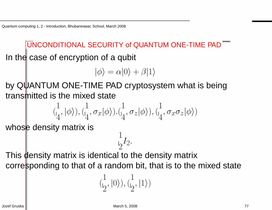
UNCONDITIONAL SECURITY of QUANTUM ONE-TIME PAD
In the case of encryption of a qubit
|φ〉 = α|0〉 + β|1〉by QUANTUM ONE-TIME PAD cryptosystem what is beingtransmitted is the mixed state
(1
4, |φ〉), (1
4, σx|φ〉).(
1
4, σz|φ〉), (
1
4, σxσz|φ〉)
whose density matrix is1
2I2.
This density matrix is identical to the density matrixcorresponding to that of a random bit, that is to the mixed state
(1
2, |0〉), (1
2, |1〉)
Jozef Gruska March 5, 2008 76
Quantum computing 1, 2 - Introduction, Bhubaneswar, School, March 2008
UNCONDITIONAL SECURITY of QUANTUM ONE-TIME PAD
In the case of encryption of a qubit
|φ〉 = α|0〉 + β|1〉by QUANTUM ONE-TIME PAD cryptosystem what is beingtransmitted is the mixed state
(1
4, |φ〉), (1
4, σx|φ〉).(
1
4, σz|φ〉), (
1
4, σxσz|φ〉)
whose density matrix is1
2I2.
This density matrix is identical to the density matrixcorresponding to that of a random bit, that is to the mixed state
(1
2, |0〉), (1
2, |1〉)
Jozef Gruska March 5, 2008 77
Quantum computing 1, 2 - Introduction, Bhubaneswar, School, March 2008
SHANNON’s THEOREMS
Shannon classical encryption theorem says thatn bits arenecessary and sufficient to encrypt securelyn bits.
Quantum version of Shannon encryption theorem says that2nclassical bits are necessary and sufficient to encrypt securely nqubits.
Jozef Gruska March 5, 2008 78
Quantum computing 1, 2 - Introduction, Bhubaneswar, School, March 2008
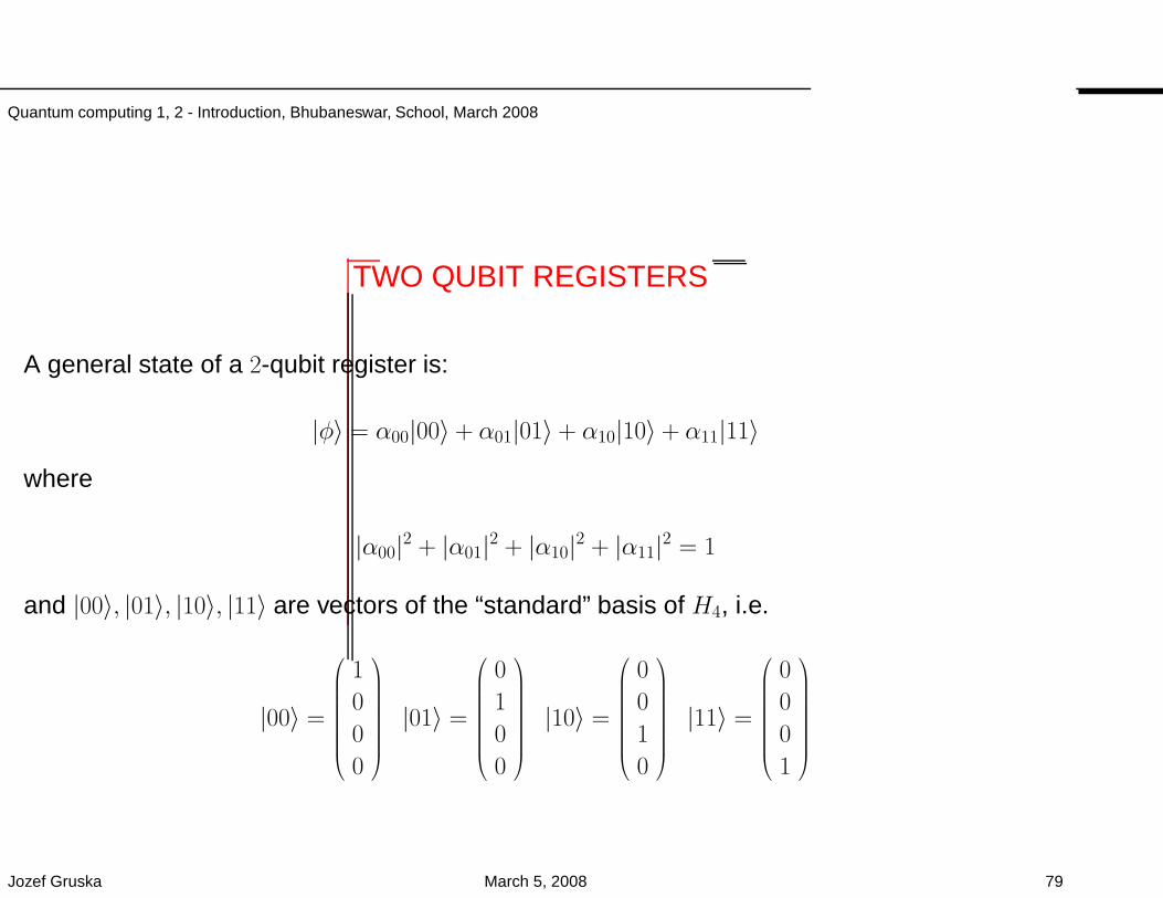
TWO QUBIT REGISTERS
A general state of a 2-qubit register is:
|φ〉 = α00|00〉 + α01|01〉 + α10|10〉 + α11|11〉
where
|α00|2 + |α01|2 + |α10|2 + |α11|2 = 1
and |00〉, |01〉, |10〉, |11〉 are vectors of the “standard” basis of H4, i.e.
|00〉 =
1
0
0
0
|01〉 =
0
1
0
0
|10〉 =
0
0
1
0
|11〉 =
0
0
0
1
Jozef Gruska March 5, 2008 79
Quantum computing 1, 2 - Introduction, Bhubaneswar, School, March 2008
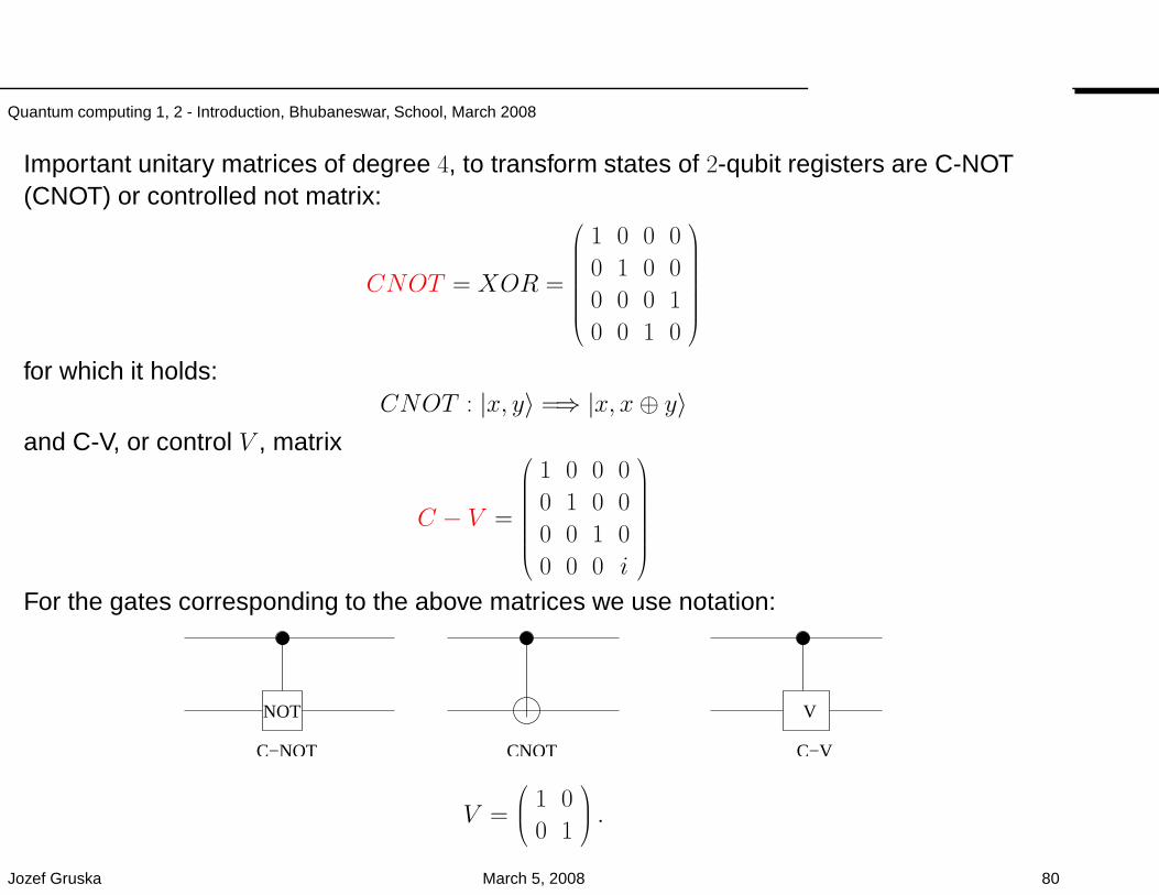
Important unitary matrices of degree 4, to transform states of 2-qubit registers are C-NOT(CNOT) or controlled not matrix:
CNOT = XOR =
1 0 0 0
0 1 0 0
0 0 0 1
0 0 1 0
for which it holds:CNOT : |x, y〉 =⇒ |x, x⊕ y〉
and C-V, or control V , matrix
C − V =
1 0 0 0
0 1 0 0
0 0 1 0
0 0 0 i
For the gates corresponding to the above matrices we use notation:
C−V
V
CNOTC−NOT
NOT
V =
1 0
0 1
.
Jozef Gruska March 5, 2008 80
Quantum computing 1, 2 - Introduction, Bhubaneswar, School, March 2008
Jozef Gruska March 5, 2008 81
Quantum computing 1, 2 - Introduction, Bhubaneswar, School, March 2008
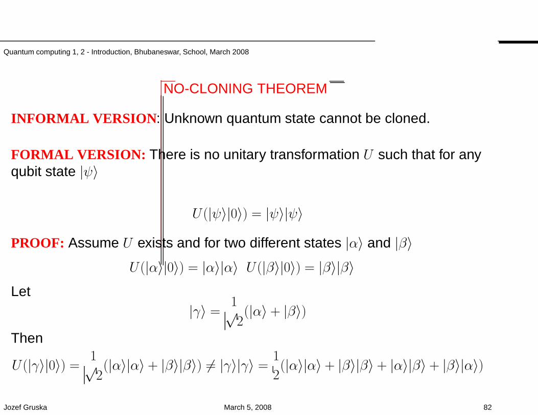
NO-CLONING THEOREM
INFORMAL VERSION : Unknown quantum state cannot be cloned.
FORMAL VERSION: There is no unitary transformation U such that for anyqubit state |ψ〉
U (|ψ〉|0〉) = |ψ〉|ψ〉
PROOF: Assume U exists and for two different states |α〉 and |β〉U (|α〉|0〉) = |α〉|α〉 U (|β〉|0〉) = |β〉|β〉
Let|γ〉 =
1√2(|α〉 + |β〉)
Then
U (|γ〉|0〉) =1√2(|α〉|α〉 + |β〉|β〉) 6= |γ〉|γ〉 =
1
2(|α〉|α〉 + |β〉|β〉 + |α〉|β〉 + |β〉|α〉)
Jozef Gruska March 5, 2008 82
Quantum computing 1, 2 - Introduction, Bhubaneswar, School, March 2008
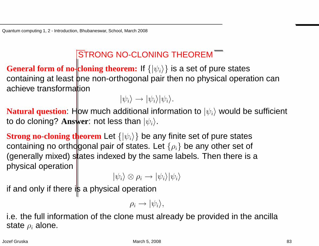
STRONG NO-CLONING THEOREM
General form of no-cloning theorem: If |ψi〉 is a set of pure statescontaining at least one non-orthogonal pair then no physical operation canachieve transformation
|ψi〉 → |ψi〉|ψi〉.Natural question: How much additional information to |ψi〉 would be sufficientto do cloning? Answer: not less than |ψi〉.Strong no-cloning theoremLet |ψi〉 be any finite set of pure statescontaining no orthogonal pair of states. Let ρi be any other set of(generally mixed) states indexed by the same labels. Then there is aphysical operation
|ψi〉 ⊗ ρi → |ψi〉|ψi〉if and only if there is a physical operation
ρi → |ψi〉,i.e. the full information of the clone must already be provided in the ancillastate ρi alone.
Jozef Gruska March 5, 2008 83
Quantum computing 1, 2 - Introduction, Bhubaneswar, School, March 2008
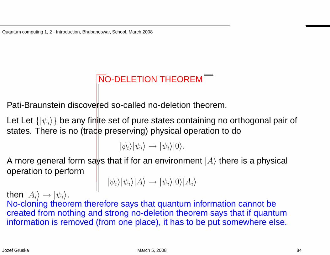
NO-DELETION THEOREM
Pati-Braunstein discovered so-called no-deletion theorem.
Let Let |ψi〉 be any finite set of pure states containing no orthogonal pair ofstates. There is no (trace preserving) physical operation to do
|ψi〉|ψi〉 → |ψi〉|0〉.A more general form says that if for an environment |A〉 there is a physicaloperation to perform
|ψi〉|ψi〉|A〉 → |ψi〉|0〉|Ai〉then |Ai〉 → |ψi〉.No-cloning theorem therefore says that quantum information cannot becreated from nothing and strong no-deletion theorem says that if quantuminformation is removed (from one place), it has to be put somewhere else.
Jozef Gruska March 5, 2008 84
Quantum computing 1, 2 - Introduction, Bhubaneswar, School, March 2008
PERMANENCE of INFORMATION
• Classical information is physical, but has no permanence.
• Permanence refers to the fact that to duplicate quantuminformation, it (second copy) must exist somewhere else in theuniverse and to eliminate quantum information, it must bemoved to somewhere else in the universe, where it still exists.
Jozef Gruska March 5, 2008 85
Quantum computing 1, 2 - Introduction, Bhubaneswar, School, March 2008
ANALYSIS of NO-CLONING and NO-DELETION THEOREMS
• Possibility of cloning or deleting would allow superluminalcommunication.
• The same is true for strong versions of no-cloning theorem -see Chakrabarthy, Pati and Adhikar 2006.
Jozef Gruska March 5, 2008 86
Quantum computing 1, 2 - Introduction, Bhubaneswar, School, March 2008
TRACING OUT OPERATION
One of the profound differences between the quantum and classical systems lies in therelation between systems and their subsystems.
As discussed below, a state of a Hilbert space H = HA⊗HB cannot be always decomposedinto states of its subspaces HA and HB. We also cannot define any natural mapping fromthe space of linear operators on H into the space of linear operators on HA (or HB).
However, density operators are much more robust and that is also one reason for theirimportance. A density operator ρ on H can be “projected” into HA by the operation oftracing out HB, to give the following density operator (for finite dimensional Hilbert spaces):
ρHA= TrHB
(ρ) =∑
|φ〉,|φ′〉∈BHA
|φ〉
∑
|ψ〉∈BHB
〈φψ|ρ|φ′ψ〉
〈φ′|,
where BHA(BHB
) is an orthonormal basis of the Hilbert space HA (of the Hilbert space HB).
Jozef Gruska March 5, 2008 87
Quantum computing 1, 2 - Introduction, Bhubaneswar, School, March 2008
TRACING OUT OPERATION II
The rule to compute ρA given on the previous slide is neither very transparent nor easy touse.
In the following an easier to use rule is will be introduced.
A meaning of the tracing out operation. If dim(A) = n, dim(B) = m, then a density matrix ρon A⊗ B, is an nm× nm matrix which can be seen as an n× n matrix consisting of m×mblocks ρij as follows:
ρ =
ρ11 . . . ρ1n
... . . .
ρn1 . . . ρnn
and in such a case
ρA =
Tr(ρ11) . . . Tr(ρ1n)
... . . . ...
Tr(ρn1) . . . Tr(ρnn)
Jozef Gruska March 5, 2008 88
Quantum computing 1, 2 - Introduction, Bhubaneswar, School, March 2008
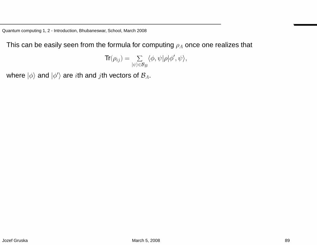
This can be easily seen from the formula for computing ρA once one realizes that
Tr(ρij) =∑
|ψ〉∈BB
〈φ, ψ|ρ|φ′, ψ〉,
where |φ〉 and |φ′〉 are ith and jth vectors of BA.
Jozef Gruska March 5, 2008 89
Quantum computing 1, 2 - Introduction, Bhubaneswar, School, March 2008
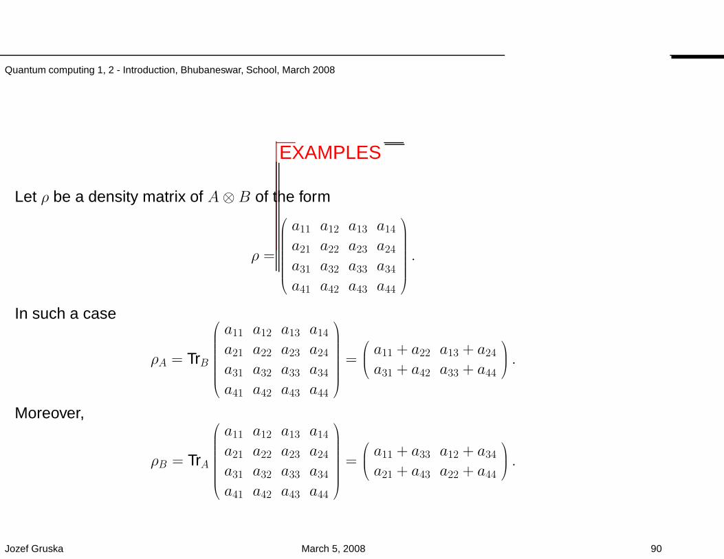
EXAMPLES
Let ρ be a density matrix of A⊗ B of the form
ρ =
a11 a12 a13 a14
a21 a22 a23 a24
a31 a32 a33 a34
a41 a42 a43 a44
.
In such a case
ρA = TrB
a11 a12 a13 a14
a21 a22 a23 a24
a31 a32 a33 a34
a41 a42 a43 a44
=
a11 + a22 a13 + a24
a31 + a42 a33 + a44
.
Moreover,
ρB = TrA
a11 a12 a13 a14
a21 a22 a23 a24
a31 a32 a33 a34
a41 a42 a43 a44
=
a11 + a33 a12 + a34
a21 + a43 a22 + a44
.
Jozef Gruska March 5, 2008 90
Quantum computing 1, 2 - Introduction, Bhubaneswar, School, March 2008
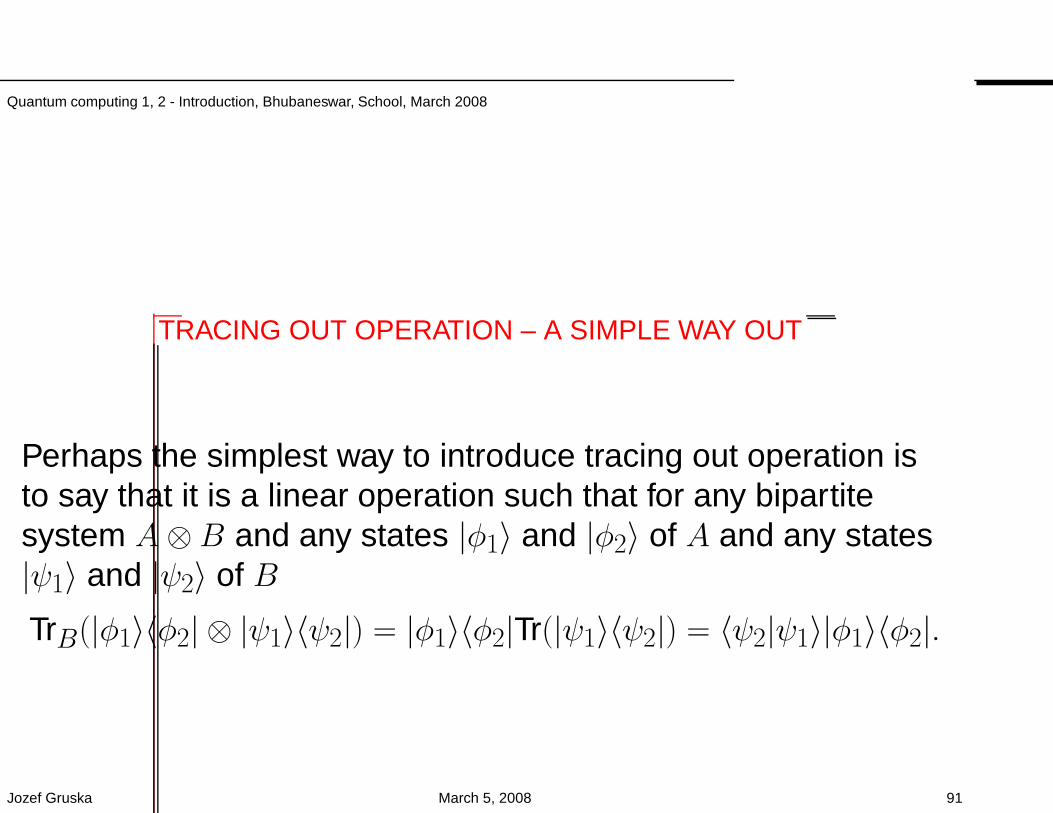
TRACING OUT OPERATION – A SIMPLE WAY OUT
Perhaps the simplest way to introduce tracing out operation isto say that it is a linear operation such that for any bipartitesystem A⊗B and any states |φ1〉 and |φ2〉 of A and any states|ψ1〉 and |ψ2〉 of B
TrB(|φ1〉〈φ2| ⊗ |ψ1〉〈ψ2|) = |φ1〉〈φ2|Tr(|ψ1〉〈ψ2|) = 〈ψ2|ψ1〉|φ1〉〈φ2|.
Jozef Gruska March 5, 2008 91
Quantum computing 1, 2 - Introduction, Bhubaneswar, School, March 2008
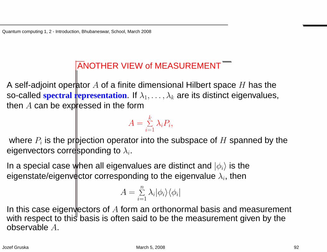
ANOTHER VIEW of MEASUREMENT
A self-adjoint operator A of a finite dimensional Hilbert space H has theso-called spectral representation. If λ1, . . . , λk are its distinct eigenvalues,then A can be expressed in the form
A =k∑
i=1λiPi,
where Pi is the projection operator into the subspace of H spanned by theeigenvectors corresponding to λi.
In a special case when all eigenvalues are distinct and |φi〉 is theeigenstate/eigenvector corresponding to the eigenvalue λi, then
A =n∑
i=1λi|φi〉〈φi|
In this case eigenvectors of A form an orthonormal basis and measurementwith respect to this basis is often said to be the measurement given by theobservable A.
Jozef Gruska March 5, 2008 92
Quantum computing 1, 2 - Introduction, Bhubaneswar, School, March 2008
IS TRACING OUT a REASONABLE OPERATION?
It is. It is a single operation with the following properties.
If we have a composed quantum system A⊗ B and we measure a state(density matrix) ρ on A⊗B with respect to an observable O⊗ IB, where O isan observable on A,
then
we get the same, in average, as if we measure ρA = TrB(ρ) only on A andwith respect only to the observable O.
Jozef Gruska March 5, 2008 93
Quantum computing 1, 2 - Introduction, Bhubaneswar, School, March 2008
QUANTUM CIRCUITS - EXAMPLES
Quantum circuits are defined in a similar way as classical onlyits gates are either unitary operations or measurements.
Hadamard gate and C-V gate form a universal set of unitarygates - using these gates one can for any unitary operation Uand ε > 0 design a quantum circuit CU that approximates Uwith precision ε.
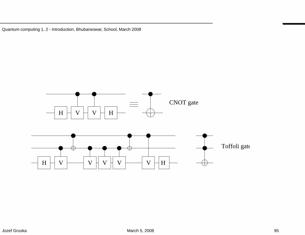
Two examples of quantum circuits for the CNOT gate and forToffoli gate:
Jozef Gruska March 5, 2008 94
Quantum computing 1, 2 - Introduction, Bhubaneswar, School, March 2008
H HV V V V V
CNOT gate
Toffoli gate
H HV V
Jozef Gruska March 5, 2008 95
Quantum computing 1, 2 - Introduction, Bhubaneswar, School, March 2008
GENERALIZATION of MACH-ZEHNDER INTERFEROMETER
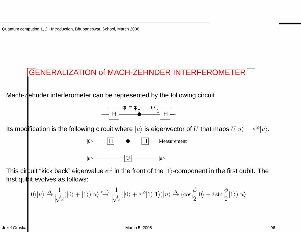
Mach-Zehnder interferometer can be represented by the following circuit
φ = φ − φ0 1Η Η
Its modification is the following circuit where |u〉 is eigenvector of U that maps U |u〉 = eiφ|u〉.
U
Η Η|0>
|u> |u>
Measurement
This circuit “kick back” eigenvalue eiφ in the front of the |1〉-component in the first qubit. Thefirst qubit evolves as follows:
|0〉|u〉 H→ 1√2(|0〉 + |1〉)|u〉 c−U→ 1√
2(|0〉 + eiφ|1〉|1〉)|u〉 H→ (cos
φ
2|0〉 + i sin
φ
2|1〉)|u〉.
Jozef Gruska March 5, 2008 96
Quantum computing 1, 2 - Introduction, Bhubaneswar, School, March 2008
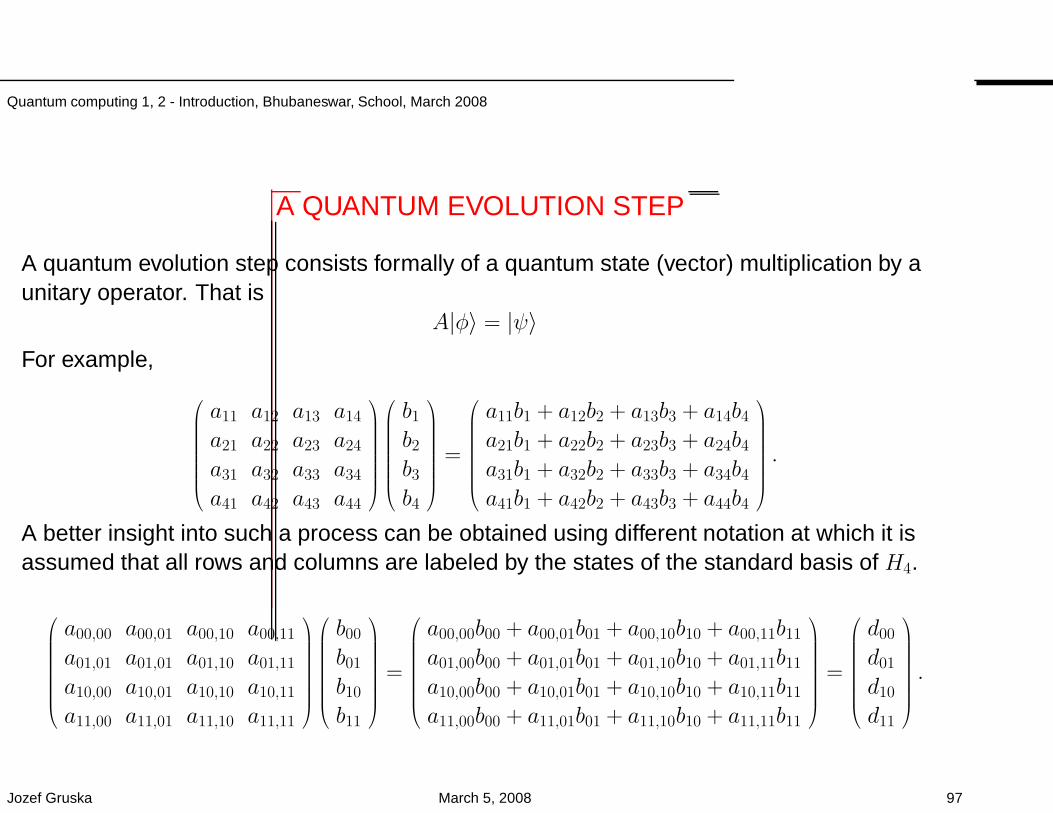
A QUANTUM EVOLUTION STEP
A quantum evolution step consists formally of a quantum state (vector) multiplication by aunitary operator. That is
A|φ〉 = |ψ〉For example,
a11 a12 a13 a14
a21 a22 a23 a24
a31 a32 a33 a34
a41 a42 a43 a44
b1b2b3b4
=
a11b1 + a12b2 + a13b3 + a14b4a21b1 + a22b2 + a23b3 + a24b4a31b1 + a32b2 + a33b3 + a34b4a41b1 + a42b2 + a43b3 + a44b4
.
A better insight into such a process can be obtained using different notation at which it isassumed that all rows and columns are labeled by the states of the standard basis of H4.
a00,00 a00,01 a00,10 a00,11
a01,01 a01,01 a01,10 a01,11
a10,00 a10,01 a10,10 a10,11
a11,00 a11,01 a11,10 a11,11
b00
b01
b10
b11
=
a00,00b00 + a00,01b01 + a00,10b10 + a00,11b11
a01,00b00 + a01,01b01 + a01,10b10 + a01,11b11
a10,00b00 + a10,01b01 + a10,10b10 + a10,11b11
a11,00b00 + a11,01b01 + a11,10b10 + a11,11b11
=
d00
d01
d10
d11
.
Jozef Gruska March 5, 2008 97
Quantum computing 1, 2 - Introduction, Bhubaneswar, School, March 2008
IMPLICATIONS FOR SECURE TRANSMISSION of QUANTUM STATES
Let us assume that an eavesdropper Eve knows that Alice is sending to Bobone quantum state from a set φ1, φ2, . . . , φn of non-orthogonal quantumstates. What she can do?
• Eve cannot make copy of the transmitted state.
• There is no measurement Eve can find out reliably which state is beingtransmitted.
• She can only measure the state being transmitted, but each such ameasurement will, with large probability, destroy the state beingtransmitted.
Intuitive conclusion There is nothing an eavesdropper can do without havinglarge probability of being detected.
Jozef Gruska March 5, 2008 98
Quantum computing 1, 2 - Introduction, Bhubaneswar, School, March 2008
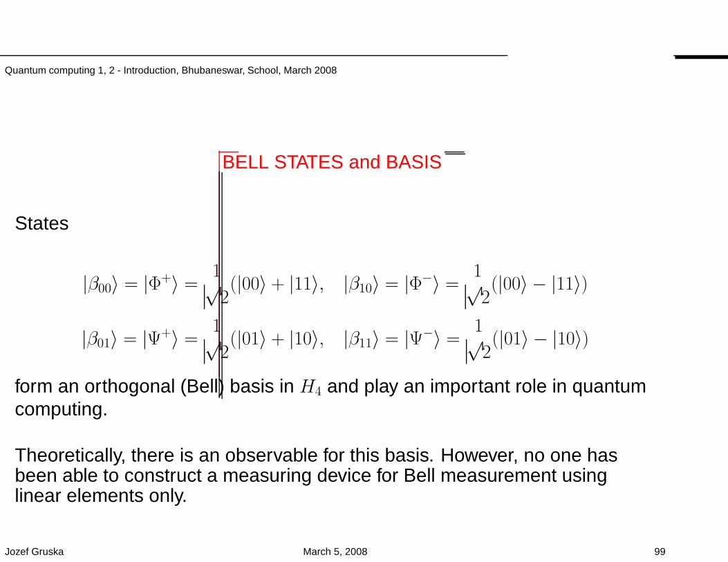
BELL STATES and BASIS
States
|β00〉 = |Φ+〉 =1√2(|00〉 + |11〉, |β10〉 = |Φ−〉 =
1√2(|00〉 − |11〉)
|β01〉 = |Ψ+〉 =1√2(|01〉 + |10〉, |β11〉 = |Ψ−〉 =
1√2(|01〉 − |10〉)
form an orthogonal (Bell) basis in H4 and play an important role in quantumcomputing.
Theoretically, there is an observable for this basis. However, no one hasbeen able to construct a measuring device for Bell measurement usinglinear elements only.
Jozef Gruska March 5, 2008 99
Quantum computing 1, 2 - Introduction, Bhubaneswar, School, March 2008
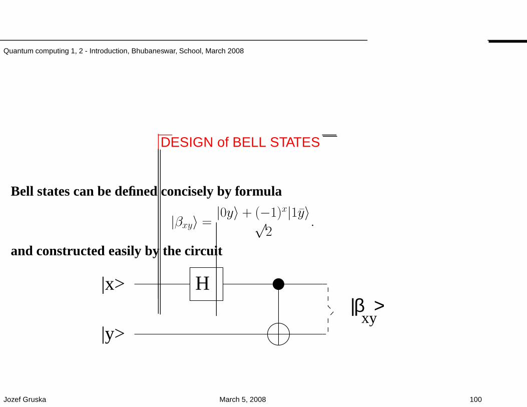
DESIGN of BELL STATES
Bell states can be defined concisely by formula
|βxy〉 =|0y〉 + (−1)x|1y〉√
2.
and constructed easily by the circuit
|x>
|y>
|β >xy
H
Jozef Gruska March 5, 2008 100
Quantum computing 1, 2 - Introduction, Bhubaneswar, School, March 2008
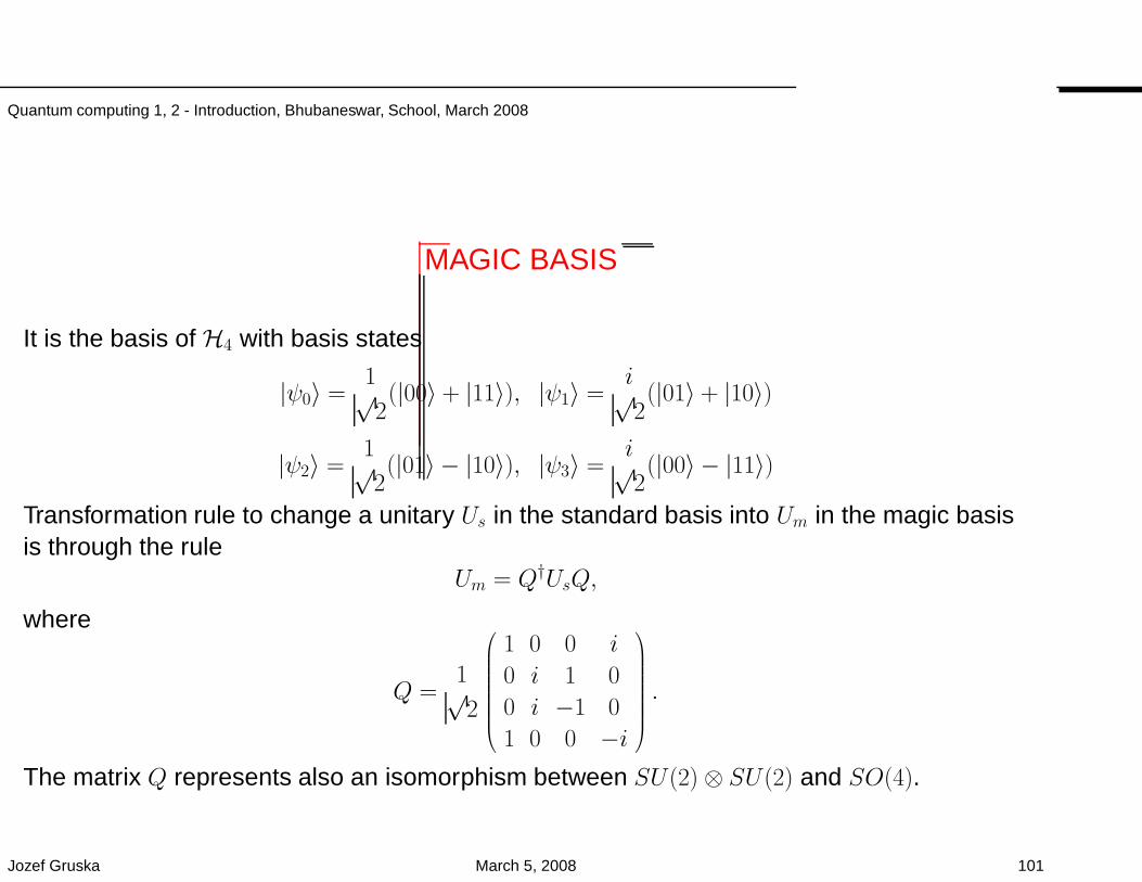
MAGIC BASIS
It is the basis of H4 with basis states
|ψ0〉 =1√2(|00〉 + |11〉), |ψ1〉 =
i√2(|01〉 + |10〉)
|ψ2〉 =1√2(|01〉 − |10〉), |ψ3〉 =
i√2(|00〉 − |11〉)
Transformation rule to change a unitary Us in the standard basis into Um in the magic basisis through the rule
Um = Q†UsQ,
where
Q =1√2
1 0 0 i
0 i 1 0
0 i −1 0
1 0 0 −i
.
The matrix Q represents also an isomorphism between SU(2)⊗ SU(2) and SO(4).
Jozef Gruska March 5, 2008 101
Quantum computing 1, 2 - Introduction, Bhubaneswar, School, March 2008
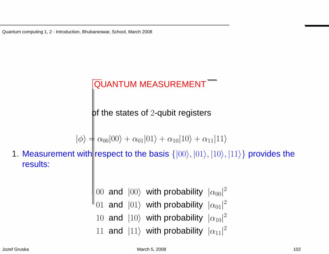
QUANTUM MEASUREMENT
of the states of 2-qubit registers
|φ〉 = α00|00〉 + α01|01〉 + α10|10〉 + α11|11〉1. Measurement with respect to the basis |00〉, |01〉, |10〉, |11〉 provides the
results:
00 and |00〉 with probability |α00|2
01 and |01〉 with probability |α01|2
10 and |10〉 with probability |α10|2
11 and |11〉 with probability |α11|2
Jozef Gruska March 5, 2008 102
Quantum computing 1, 2 - Introduction, Bhubaneswar, School, March 2008
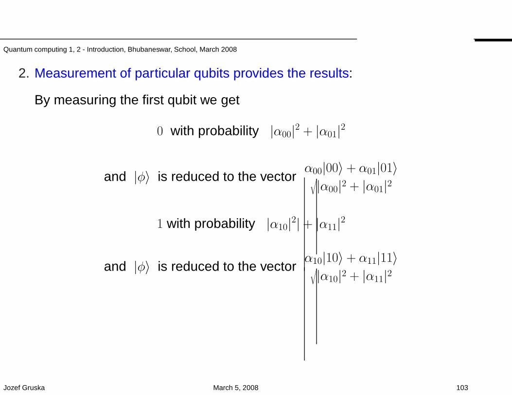
2. Measurement of particular qubits provides the results:
By measuring the first qubit we get
0 with probability |α00|2 + |α01|2
and |φ〉 is reduced to the vectorα00|00〉 + α01|01〉
√
|α00|2 + |α01|2
1 with probability |α10|2| + |α11|2
and |φ〉 is reduced to the vectorα10|10〉 + α11|11〉
√
|α10|2 + |α11|2
Jozef Gruska March 5, 2008 103
Quantum computing 1, 2 - Introduction, Bhubaneswar, School, March 2008
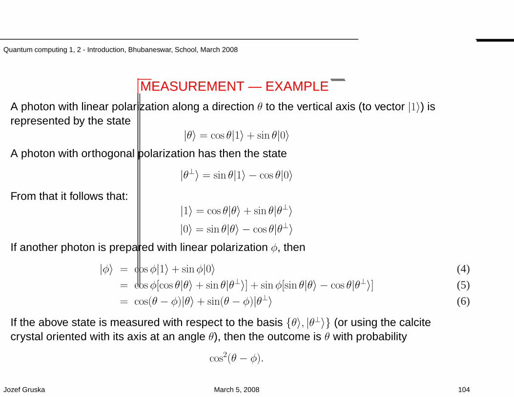
MEASUREMENT — EXAMPLE
A photon with linear polarization along a direction θ to the vertical axis (to vector |1〉) isrepresented by the state
|θ〉 = cos θ|1〉 + sin θ|0〉A photon with orthogonal polarization has then the state
|θ⊥〉 = sin θ|1〉 − cos θ|0〉
From that it follows that:|1〉 = cos θ|θ〉 + sin θ|θ⊥〉|0〉 = sin θ|θ〉 − cos θ|θ⊥〉
If another photon is prepared with linear polarization φ, then
|φ〉 = cosφ|1〉 + sinφ|0〉 (4)
= cosφ[cos θ|θ〉 + sin θ|θ⊥〉] + sinφ[sin θ|θ〉 − cos θ|θ⊥〉] (5)
= cos(θ − φ)|θ〉 + sin(θ − φ)|θ⊥〉 (6)
If the above state is measured with respect to the basis θ〉, |θ⊥〉 (or using the calcitecrystal oriented with its axis at an angle θ), then the outcome is θ with probability
cos2(θ − φ).
Jozef Gruska March 5, 2008 104
Quantum computing 1, 2 - Introduction, Bhubaneswar, School, March 2008
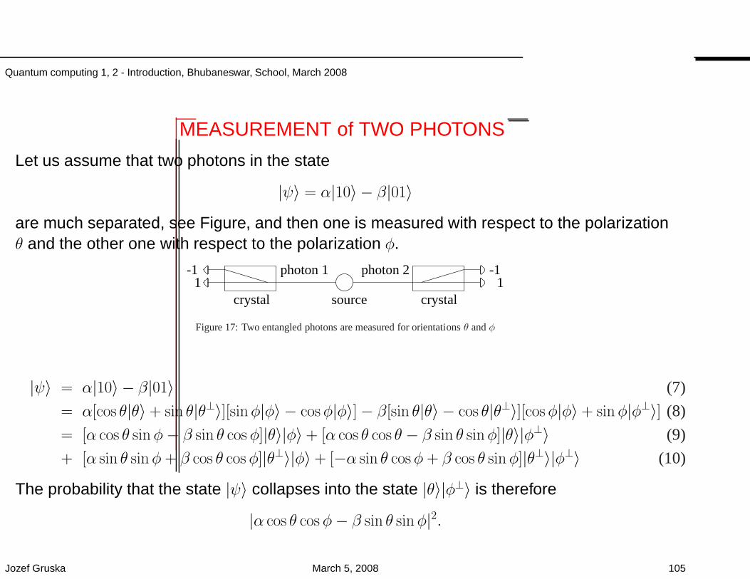
MEASUREMENT of TWO PHOTONS
Let us assume that two photons in the state
|ψ〉 = α|10〉 − β|01〉
are much separated, see Figure, and then one is measured with respect to the polarizationθ and the other one with respect to the polarization φ.
-1 1
-1 1
crystal crystalsource
photon 1 photon 2
Figure 17: Two entangled photons are measured for orientationsθ andφ
|ψ〉 = α|10〉 − β|01〉 (7)
= α[cos θ|θ〉 + sin θ|θ⊥〉][sinφ|φ〉 − cosφ|φ〉]− β[sin θ|θ〉 − cos θ|θ⊥〉][cosφ|φ〉 + sinφ|φ⊥〉] (8)
= [α cos θ sinφ− β sin θ cosφ]|θ〉|φ〉 + [α cos θ cos θ − β sin θ sinφ]|θ〉|φ⊥〉 (9)
+ [α sin θ sinφ + β cos θ cosφ]|θ⊥〉|φ〉 + [−α sin θ cosφ + β cos θ sinφ]|θ⊥〉|φ⊥〉 (10)
The probability that the state |ψ〉 collapses into the state |θ〉|φ⊥〉 is therefore
|α cos θ cosφ− β sin θ sinφ|2.
Jozef Gruska March 5, 2008 105
Quantum computing 1, 2 - Introduction, Bhubaneswar, School, March 2008
QUANTUM ENTANGLEMENT I
The concept of entanglement is primarily concerned with states ofmultipartite systems.
For a bipartite quantum system H = HA ⊗HB, we say that its state |Φ〉 is anentangled state if it cannot be decomposed into a tensor product of a statefrom HA and a state from HB.
For example, it is easy to verify that a two-qubit state
|φ〉 = a|00〉+ b|01〉 + c|10〉 + d|11〉,is not entangled, that is
|φ〉 = (x1|0〉 + y1|1〉)⊗ (x2|0〉 + y2|1〉)if and only if ab = x2
y2= c
d, that is if
ad− bc = 0.
Therefore, all Bell states are entangled, and they are important examples ofentangled states.
Jozef Gruska March 5, 2008 106
Quantum computing 1, 2 - Introduction, Bhubaneswar, School, March 2008
QUANTUM ENTANGLEMENT - BASIC DEFINITIONS
The concept of entanglement is primarily concerned with the states ofmultipartite systems.
For a bipartite quantum system H = HA ⊗HB, a pure state |Φ〉 is calledentangled if it cannot be decomposed into a tensor product of a state fromHA and a state from HB.
A mixed state (density matrix) ρ of H is called entangled if ρ cannot bewritten in the form
ρ =k∑
i=1piρA,i ⊗ ρB,i
where ρA,i (ρB,i) are density matrices in HA (in HB) and ∑ki=1 pi = 1, pi > 0.
Jozef Gruska March 5, 2008 107
Quantum computing 1, 2 - Introduction, Bhubaneswar, School, March 2008
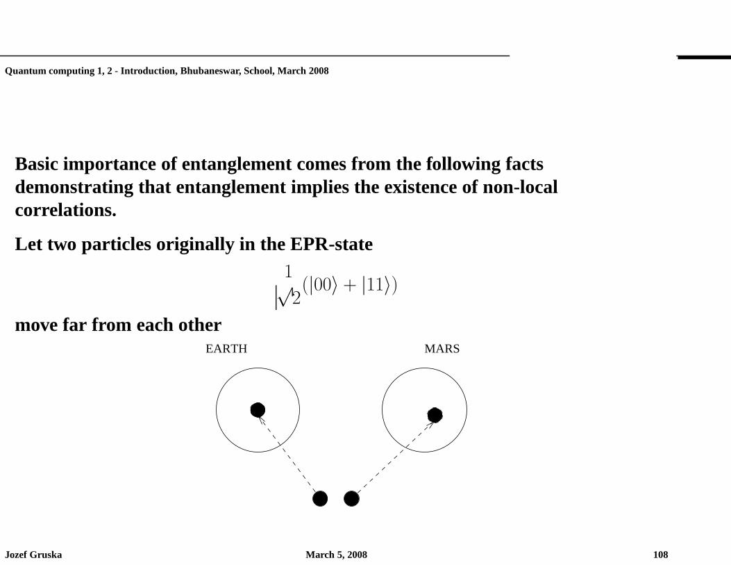
Basic importance of entanglement comes from the following factsdemonstrating that entanglement implies the existence of non-localcorrelations.
Let two particles originally in the EPR-state1√2(|00〉 + |11〉)
move far from each otherMARSEARTH
Jozef Gruska March 5, 2008 108
Quantum computing 1, 2 - Introduction, Bhubaneswar, School, March 2008
then measurement of any one of these particles makes theEPR-state to collapse, randomly, either to one of the states|00〉 or|11〉. As the classical outcomes both parties get at theirmeasurements, no matter when they make them, the sameoutcomes.
Einstein called this phenomenon “spooky action at a distance”because measurement in one place seems to have an instantaneous(non-local) effect at the other (very distant) place.
Jozef Gruska March 5, 2008 109
Quantum computing 1, 2 - Introduction, Bhubaneswar, School, March 2008
CREATION of ENTANGLED STATES
Entangled states are gold mine for QIPC, but their creation is very difficult.This is natural because particles in an entangled states should exhibitnon-local correlations no matter how far they are.
Basic methods to create entangled states:
• Using special physical processes, for example parametricdown-conversion. (Nowadays one can create in one second millionmaximally entangled states with 99% “precision” (fidelity)).
• Using “entangling” quantum operations. For example
CNOT((1√2(|0〉 + |1〉))⊗ |0〉) =
1√2(|00〉 + |11〉)
• Using entanglement swapping.
Jozef Gruska March 5, 2008 110
Quantum computing 1, 2 - Introduction, Bhubaneswar, School, March 2008
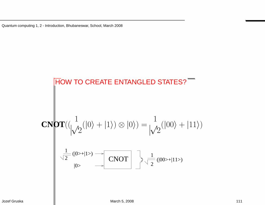
HOW TO CREATE ENTANGLED STATES?
CNOT((1√2(|0〉 + |1〉)⊗ |0〉) =
1√2(|00〉 + |11〉)
1
2(|00>+|11>)CNOT
(|0>+|1>)12
|0>
Jozef Gruska March 5, 2008 111
Quantum computing 1, 2 - Introduction, Bhubaneswar, School, March 2008
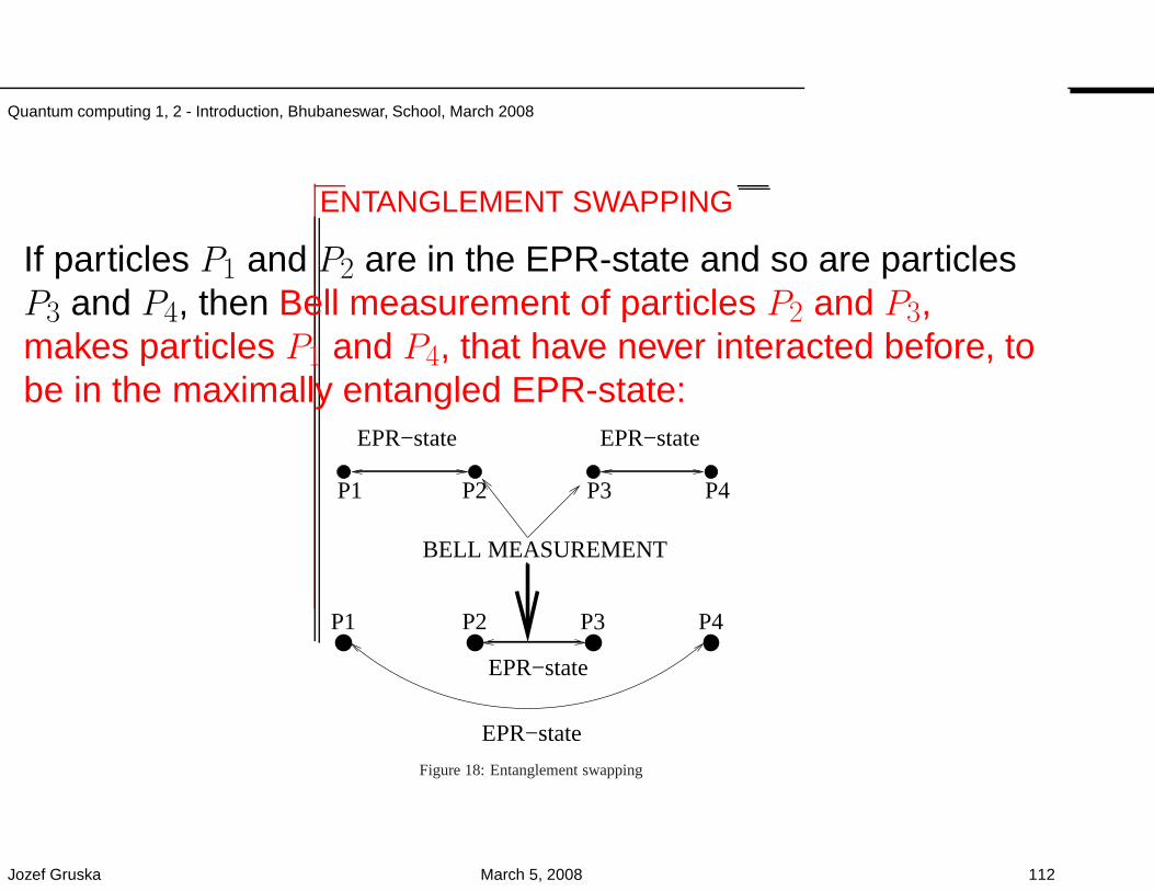
ENTANGLEMENT SWAPPING
If particles P1 and P2 are in the EPR-state and so are particlesP3 and P4, then Bell measurement of particles P2 and P3,makes particles P1 and P4, that have never interacted before, tobe in the maximally entangled EPR-state:
EPR−state EPR−state
BELL MEASUREMENT
EPR−state
EPR−state
P1 P2 P3 P4
P1 P2 P3 P4
Figure 18: Entanglement swapping
Jozef Gruska March 5, 2008 112
Quantum computing 1, 2 - Introduction, Bhubaneswar, School, March 2008
QUANTUM NON-LOCALITY
• Physics was non-local since Newton’s time, with exception ofthe period 1915-1925.
• Newton has fully realized counter-intuitive consequences ofthe non-locality his theory implied.
• Einstein has realized the non-locality quantum mechanicsimply, but it does not seem that he realized that entanglementbased non-locality does not violate no-signaling assumption.
• Recently, attempts started to study stronger non-signalingnon-locality than the one quantum mechanics allows.
Jozef Gruska March 5, 2008 113
Quantum computing 1, 2 - Introduction, Bhubaneswar, School, March 2008
NON-LOCALITY in NEWTON’s THEORY
Newton realized that his theory concerning gravity allowsnon-local effect. Namely, that
if a stone is moved on the moon, then weight of all of us, hereon the earth, isimmediately modified.
Jozef Gruska March 5, 2008 114
Quantum computing 1, 2 - Introduction, Bhubaneswar, School, March 2008
NEWTON’s words
The consequences of current theory that implies that gravityshould be innate, inherent and essential to Matter, so that anyBody may act upon another at a Distance throw a Vacuum,without the mediation of any thing else, by and through whichtheir Action and Force may be conveyed from one to another, isto me so great an Absurdity, that I believe no Man who has inphilosophical Matters a competent Faculty of thinking, can everfall unto it.Gravity must be caused by an Agent acting constantlyaccording certain Laws, but whether this Agent be material orimmaterial, I have left to the Consideration of my Readers.
Jozef Gruska March 5, 2008 115
Quantum computing 1, 2 - Introduction, Bhubaneswar, School, March 2008
POWER of ENTANGLEMENT
After its discovery, entanglement and its non-locality impacts have beenseen as a peculiarity of the existing quantum theory that needs somemodification to get rid of them, as a source of all kind mysteries andcounter-intuitive consequences.
Currently, after the discovery of quantum teleportation and of such powerfulquantum algorithms as Shor’s factorization algorithm, entanglement is seenand explored as a new and powerful quantum resource that allows
• to perform tasks that are not possible otherwise;
• to speed-up much some computations and to economize (evenexponentially) some communications;
• to increase capacity of (quantum) communication channels;
• to implement perfectly secure information transmissions;
• to develop a new, better, information based, understanding of the keyquantum phenomena and by that, a deeper, information processing based,understanding of Nature.
Jozef Gruska March 5, 2008 116
Quantum computing 1, 2 - Introduction, Bhubaneswar, School, March 2008
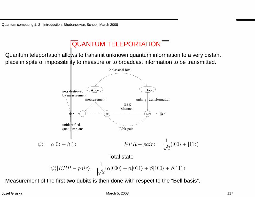
QUANTUM TELEPORTATION
Quantum teleportation allows to transmit unknown quantum information to a very distantplace in spite of impossibility to measure or to broadcast information to be transmitted.
gets destroyedby measurement
unidentifiedquantum state
channelEPR
Alice Bob
2 classical bits
|M> |M> |ψ>|ψ>
measu rement unitary transformation
EPR-pair
|ψ〉 = α|0〉 + β|1〉 |EPR− pair〉 =1√2(|00〉 + |11〉)
Total state
|ψ〉|EPR− pair〉 =1√2(α|000〉 + α|011〉 + β|100〉 + β|111〉
Measurement of the first two qubits is then done with respect to the “Bell basis”.
Jozef Gruska March 5, 2008 117
Quantum computing 1, 2 - Introduction, Bhubaneswar, School, March 2008
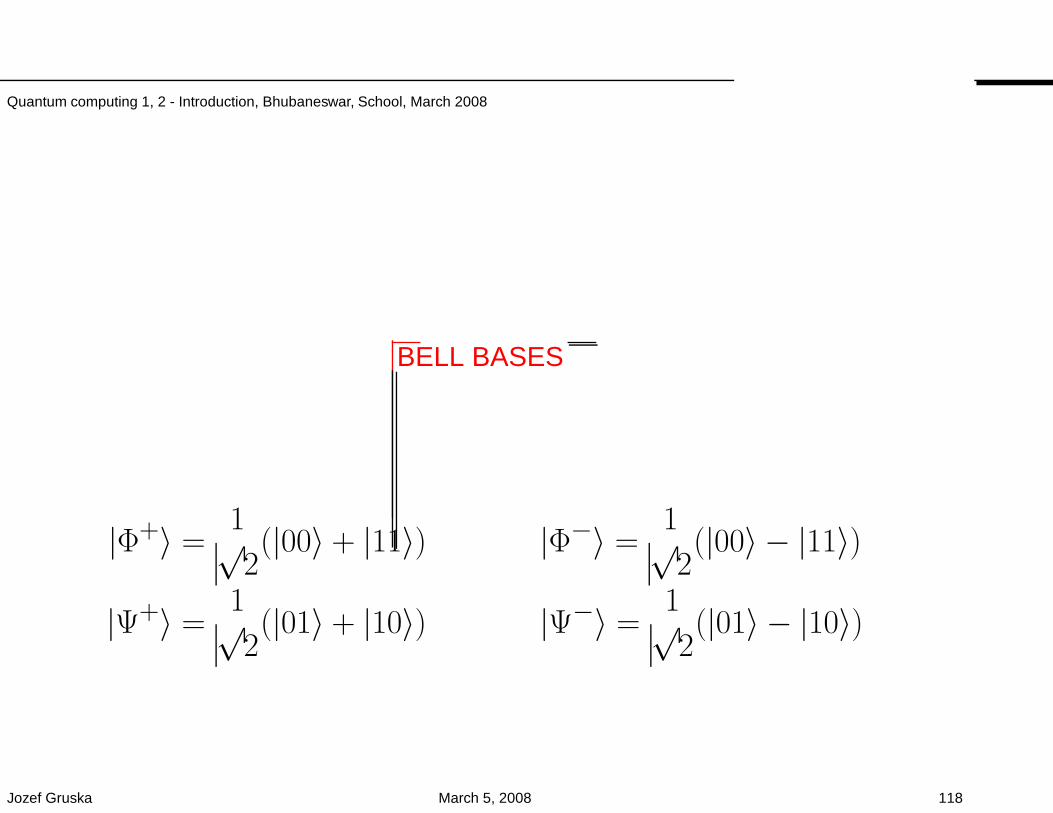
BELL BASES
|Φ+〉 =1√2(|00〉 + |11〉) |Φ−〉 =
1√2(|00〉 − |11〉)
|Ψ+〉 =1√2(|01〉 + |10〉) |Ψ−〉 =
1√2(|01〉 − |10〉)
Jozef Gruska March 5, 2008 118
Quantum computing 1, 2 - Introduction, Bhubaneswar, School, March 2008
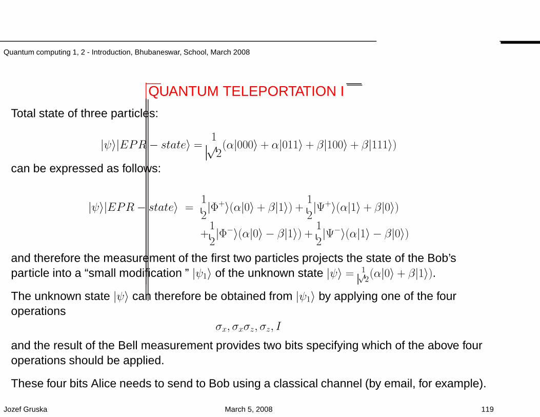
QUANTUM TELEPORTATION I
Total state of three particles:
|ψ〉|EPR− state〉 =1√2(α|000〉 + α|011〉 + β|100〉 + β|111〉)
can be expressed as follows:
|ψ〉|EPR− state〉 =1
2|Φ+〉(α|0〉 + β|1〉) +
1
2|Ψ+〉(α|1〉 + β|0〉)
+1
2|Φ−〉(α|0〉 − β|1〉) +
1
2|Ψ−〉(α|1〉 − β|0〉)
and therefore the measurement of the first two particles projects the state of the Bob’sparticle into a “small modification ” |ψ1〉 of the unknown state |ψ〉 = 1√
2(α|0〉 + β|1〉).
The unknown state |ψ〉 can therefore be obtained from |ψ1〉 by applying one of the fouroperations
σx, σxσz, σz, I
and the result of the Bell measurement provides two bits specifying which of the above fouroperations should be applied.
These four bits Alice needs to send to Bob using a classical channel (by email, for example).
Jozef Gruska March 5, 2008 119
Quantum computing 1, 2 - Introduction, Bhubaneswar, School, March 2008
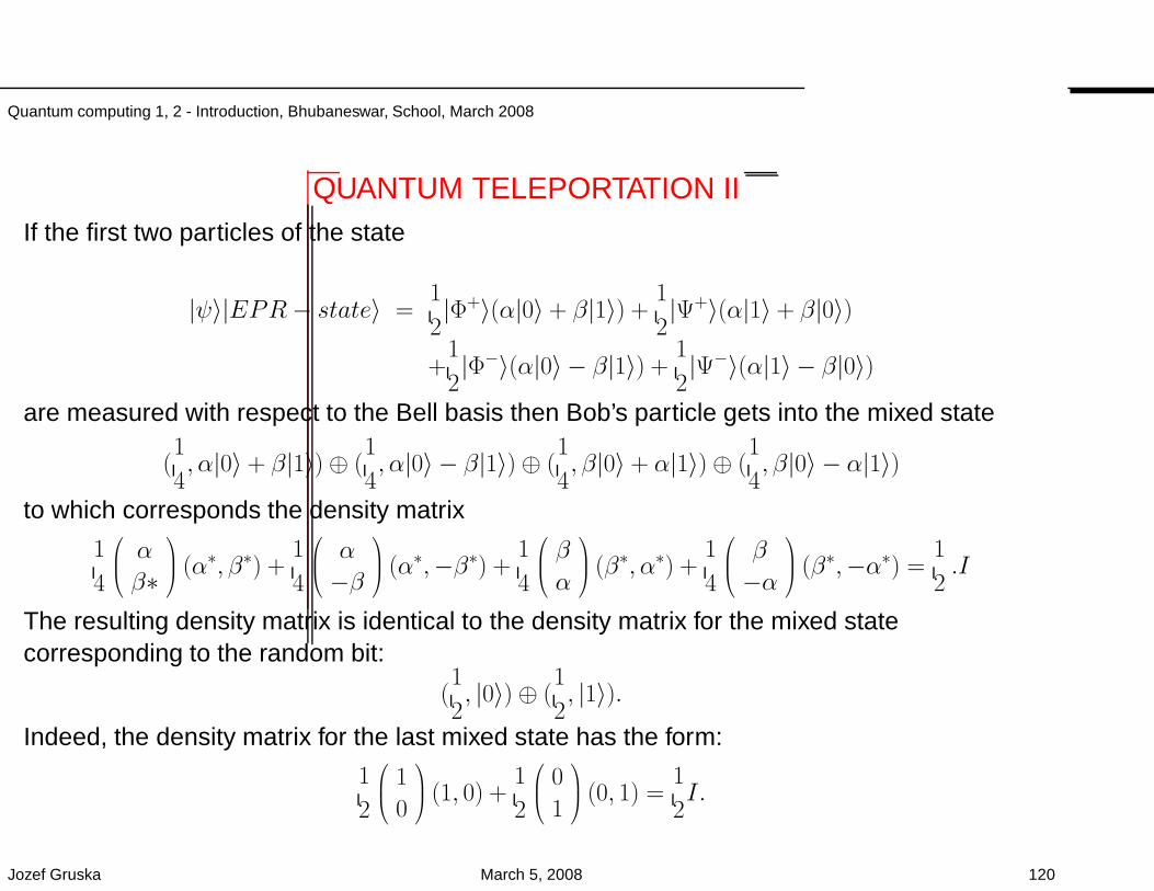
QUANTUM TELEPORTATION IIIf the first two particles of the state
|ψ〉|EPR− state〉 =1
2|Φ+〉(α|0〉 + β|1〉) +
1
2|Ψ+〉(α|1〉 + β|0〉)
+1
2|Φ−〉(α|0〉 − β|1〉) +
1
2|Ψ−〉(α|1〉 − β|0〉)
are measured with respect to the Bell basis then Bob’s particle gets into the mixed state
(1
4, α|0〉 + β|1〉)⊕ (
1
4, α|0〉 − β|1〉)⊕ (
1
4, β|0〉 + α|1〉)⊕ (
1
4, β|0〉 − α|1〉)
to which corresponds the density matrix
1
4
α
β∗
(α∗, β∗) +1
4
α
−β
(α∗,−β∗) +1
4
β
α
(β∗, α∗) +1
4
β
−α
(β∗,−α∗) =1
2.I
The resulting density matrix is identical to the density matrix for the mixed statecorresponding to the random bit:
(1
2, |0〉)⊕ (
1
2, |1〉).
Indeed, the density matrix for the last mixed state has the form:
1
2
1
0
(1, 0) +1
2
0
1
(0, 1) =1
2I.
Jozef Gruska March 5, 2008 120
Quantum computing 1, 2 - Introduction, Bhubaneswar, School, March 2008
QUANTUM TELEPORTATION — COMMENTS
• Alice can be seen as dividing information contained in|ψ〉 into
quantum information - transmitted through EPR channelandclassical information - transmitted through a classical channel
• In a quantum teleportation an unknown quantum state|φ〉 can bedisassembled into, and later reconstructed from, two classical bit-states andan maximally entangled pure quantum state.
• Using quantum teleportation an unknown quantum state can beteleportedfrom one place to another by a sender who does not need to know —forteleportation itself — neither the state to be teleported nor the location of theintended receiver.
• One can also see quantum teleportation as a protocol that allows one toteleport all characteristics of an object, embedded in somematter andenergy, and localized at one place to another piece of energyand matterlocated at a distance.
Jozef Gruska March 5, 2008 121
Quantum computing 1, 2 - Introduction, Bhubaneswar, School, March 2008
• The teleportation procedure cannot be used to transmit information fasterthan light
butit can be argued that quantum information presented in unknown state istransmitted instantaneously (except two random bits to be transmitted at thespeed of light at most).
• EPR channel is irreversibly destroyed during the teleportation process.
• One can also see quantum teleportation as a protocol that allows one toteleport all characteristics of an object embedded in some matter and energylocalized at one place to another piece of energy and matter located at adistance.
Jozef Gruska March 5, 2008 122
Quantum computing 1, 2 - Introduction, Bhubaneswar, School, March 2008
QUANTUM TELEPORTATION - GENERALISATIONS
•One can teleport also qudits from Hd. In such a case Aliceand Bob have to share a maximally entangled state in Hd ( anatural generalisation of the EPR-state) and measurement isperformed in a (naturally) generalised Bell basis.
• Teleportation can be done also if the state Alice and Bobshare is not maximally entangled or even a mixed state. Insuch a case there is a price to pay, either concerning fidelity(quality of teleportation) or probability (of perfect result (seeAgrawal. Pati - quant-ph/0611115.
Jozef Gruska March 5, 2008 123
Quantum computing 1, 2 - Introduction, Bhubaneswar, School, March 2008
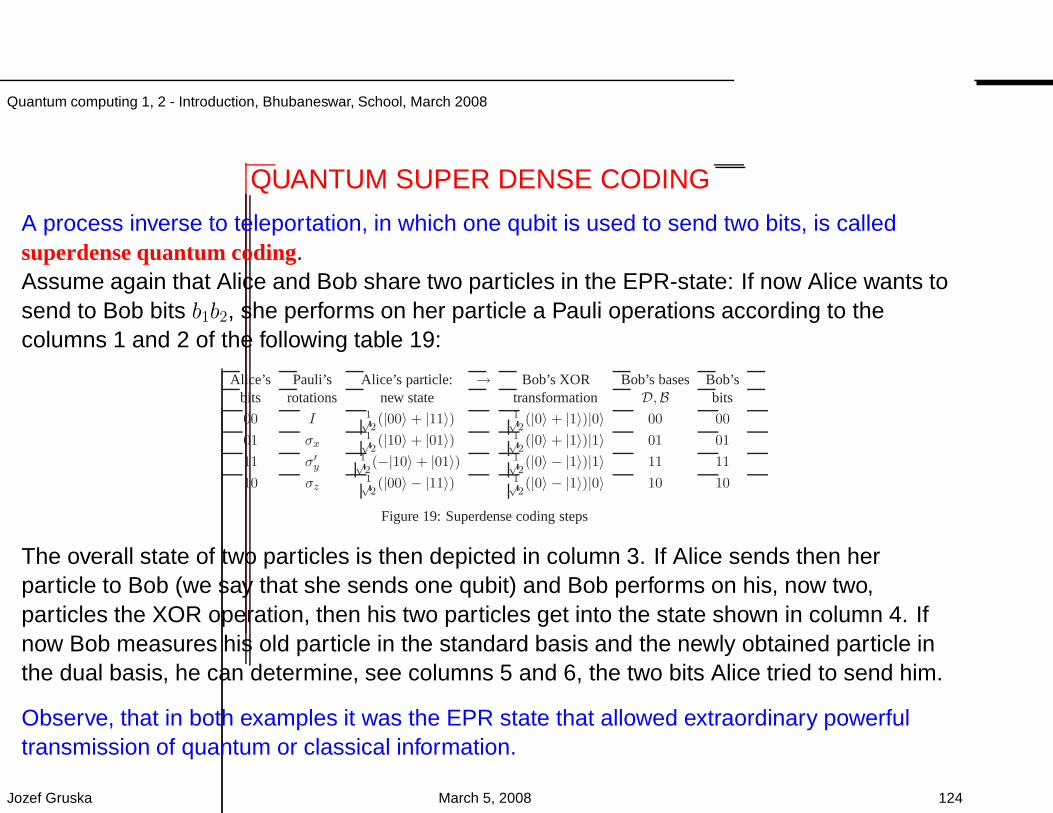
QUANTUM SUPER DENSE CODING
A process inverse to teleportation, in which one qubit is used to send two bits, is calledsuperdense quantum coding.Assume again that Alice and Bob share two particles in the EPR-state: If now Alice wants tosend to Bob bits b1b2, she performs on her particle a Pauli operations according to thecolumns 1 and 2 of the following table 19:
Alice’s Pauli’s Alice’s particle: → Bob’s XOR Bob’s bases Bob’sbits rotations new state transformation D,B bits
00 I 1√2(|00〉 + |11〉) 1√
2(|0〉 + |1〉)|0〉 00 00
01 σx1√2(|10〉 + |01〉) 1√
2(|0〉 + |1〉)|1〉 01 01
11 σ′y
1√2(−|10〉 + |01〉) 1√
2(|0〉 − |1〉)|1〉 11 11
10 σz1√2(|00〉 − |11〉) 1√
2(|0〉 − |1〉)|0〉 10 10
Figure 19: Superdense coding steps
The overall state of two particles is then depicted in column 3. If Alice sends then herparticle to Bob (we say that she sends one qubit) and Bob performs on his, now two,particles the XOR operation, then his two particles get into the state shown in column 4. Ifnow Bob measures his old particle in the standard basis and the newly obtained particle inthe dual basis, he can determine, see columns 5 and 6, the two bits Alice tried to send him.
Observe, that in both examples it was the EPR state that allowed extraordinary powerfultransmission of quantum or classical information.
Jozef Gruska March 5, 2008 124
Quantum computing 1, 2 - Introduction, Bhubaneswar, School, March 2008
QUANTUM PSEUDO-TELEPATHY
Using entangled states various effects can be produced that resemble telepathy.
Example - Stage telepathy
Two players, Alice and Bob, are on a stage, see Figure 20, very far from each other (so farthat they cannot communicate), and they are simultaneously, but independently andrandomly asked again and again, by a moderator, either a “food question” or a “colorquestion”.
• FOOD question: What is your favorite meal?
ANSWER has to be either carrot or peas.
• COLOR question: What is your favorite color?
ANSWER has to be either greenor red.
Jozef Gruska March 5, 2008 125
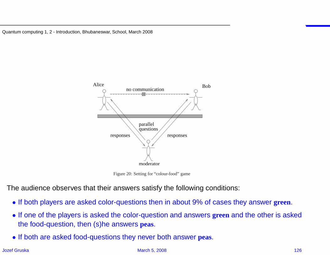
Quantum computing 1, 2 - Introduction, Bhubaneswar, School, March 2008
responses
no communicationAlice Bob
moderator
parallelquestions
responses
Figure 20: Setting for “colour-food” game
The audience observes that their answers satisfy the following conditions:
• If both players are asked color-questions then in about 9% of cases they answer green.
• If one of the players is asked the color-question and answers greenand the other is askedthe food-question, then (s)he answers peas.
• If both are asked food-questions they never both answer peas.
Jozef Gruska March 5, 2008 126
Quantum computing 1, 2 - Introduction, Bhubaneswar, School, March 2008
It is not difficult to show that within the classical physics there is no way that Alice and Bobcould invent a strategy for their answers, before they went to the stage, in such a way thatthe above mentioned behavior of them would be observed. However, there is a quantumsolution, and actually quite a simple one.
Jozef Gruska March 5, 2008 127
Quantum computing 1, 2 - Introduction, Bhubaneswar, School, March 2008
SOLUTIONLet |p〉 and |c〉 be two arbitrary orthogonal states in the two-dimensional Hilbert space H2,and let
|r〉 = a|p〉 + b|c〉,|g〉 = b|p〉 − a|c〉
be two new (orthogonal) states.
Let Alice and Bob, at the very beginning, before they go to the stage, create a large numberof pairs of particles in the state
|ψ〉 = N(|r〉|r〉 − a2|p〉|p〉),where N is a normalization factor, and let later each of them takes his/her particle fromeach pair with him/her to the stage.
If any of them is asked the color-question, then (s)he measures his/her particle with respectto the |r〉, |g〉-basis and answers in accordance with the result of measurement.
If any of them is asked the food-question (s)he measures his/her particle with respect to the|p〉, |c〉-basis and responds in accordance with the result of measurement.
It is a not difficult exercise to show that in this way Alice’s and Bob’s responses follow therules described above (9% comes from an optimization in one case).
Jozef Gruska March 5, 2008 128
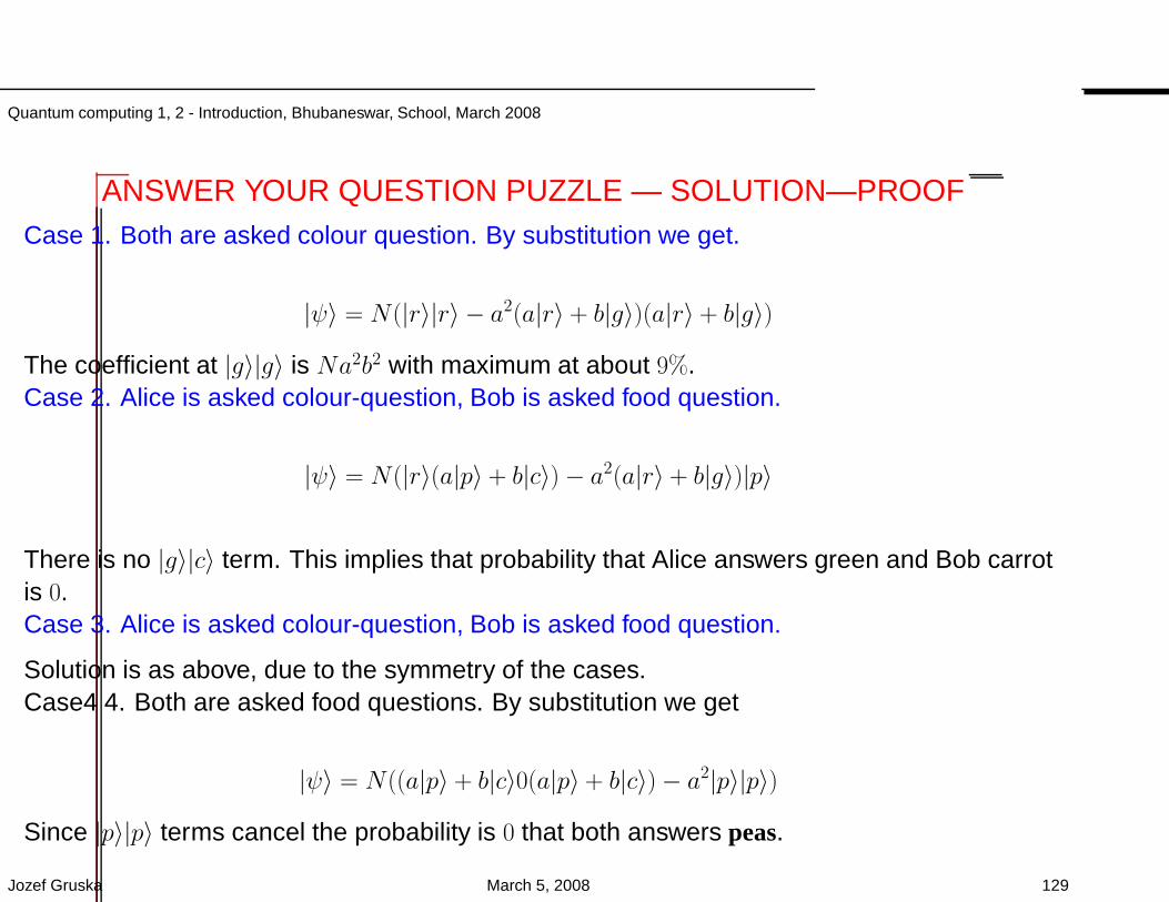
Quantum computing 1, 2 - Introduction, Bhubaneswar, School, March 2008
ANSWER YOUR QUESTION PUZZLE — SOLUTION—PROOFCase 1. Both are asked colour question. By substitution we get.
|ψ〉 = N(|r〉|r〉 − a2(a|r〉 + b|g〉)(a|r〉 + b|g〉)
The coefficient at |g〉|g〉 is Na2b2 with maximum at about 9%.Case 2. Alice is asked colour-question, Bob is asked food question.
|ψ〉 = N(|r〉(a|p〉 + b|c〉)− a2(a|r〉 + b|g〉)|p〉
There is no |g〉|c〉 term. This implies that probability that Alice answers green and Bob carrotis 0.Case 3. Alice is asked colour-question, Bob is asked food question.
Solution is as above, due to the symmetry of the cases.Case4 4. Both are asked food questions. By substitution we get
|ψ〉 = N((a|p〉 + b|c〉0(a|p〉+ b|c〉)− a2|p〉|p〉)
Since |p〉|p〉 terms cancel the probability is 0 that both answers peas.
Jozef Gruska March 5, 2008 129
Quantum computing 1, 2 - Introduction, Bhubaneswar, School, March 2008
WHAT ARE QUANTUM OPERATIONS?
The main question we deal with in this section is very fundamental.What are physically realizable operations one can perform (at leasttheoretically) on (mixed) states (to get again (mixed) states )?
In closed quantum systems unitary operations are actually the only quantumoperations that are available. Measurements are actually outside of theclosed system framework, an interface from quantum to classical world, butsurely they are operations we consider as physically realizable.
Of main importance are quantum operations in open quantum systems.Actually, all actions that are performed in open quantum systems arequantum operations: unitary operations, measurements, channeltransmissions, flow of time, noise impacts, ....
The concept of quantum operations is therefore very general and veryfundamental.
It is perhaps a bit surprising, but actually nice, useful and natural, that wecan actually study and consider open quantum systems in the framework of
Jozef Gruska March 5, 2008 130
Quantum computing 1, 2 - Introduction, Bhubaneswar, School, March 2008
closed quantum systems.We can consider as the basic setting that our(principal) quantum system and its environment form a closed quantumsystem in which we operate.
The requirement to consider only physically realizable (at least theoretically)operation is, of course, logical. As we shall see this question has, in a senseand at least theoretically, clear and simple answer. They are, as discussedlater, trace preserving completely positive linear maps.
Jozef Gruska March 5, 2008 131
Quantum computing 1, 2 - Introduction, Bhubaneswar, School, March 2008
THREE APPROACHES
There are basically three main approaches to define what are “physicallyrealizable quantum operations” (superoperators) E .
A physically motivated axiomatic approach says that for a Hilbert space Hwe should consider as physically realizable operations maps B(H)→ B(H)which are consistent with the (statistical) interpretation of quantum theory.That is map that are linear (to preserve superpositions), positive and tracepreserving (to map density operators to density operators) and actuallycompletely positive.
A pragmatic approach says that superoperators are those operations thatcan be combined from unitary operations, adding ancillas, performing(non-selective) projective measurement and discarding subsystems(ancillas), by performing a tracing out operation.
Jozef Gruska March 5, 2008 132
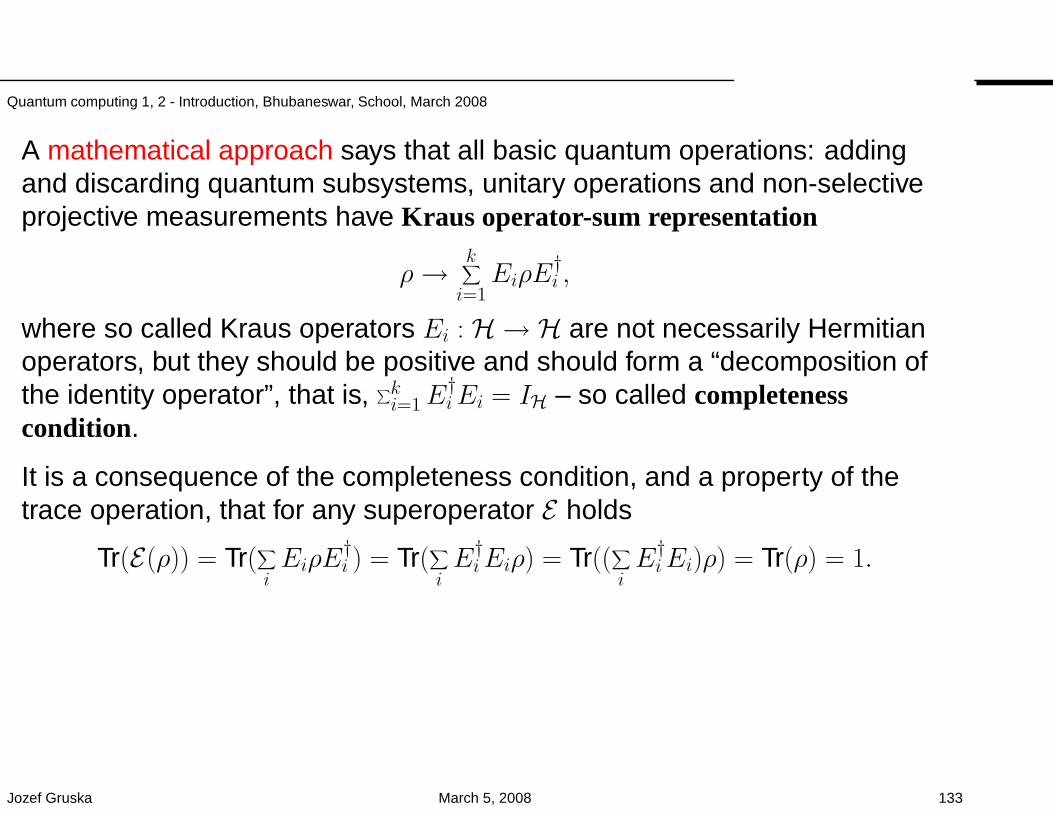
Quantum computing 1, 2 - Introduction, Bhubaneswar, School, March 2008
A mathematical approach says that all basic quantum operations: addingand discarding quantum subsystems, unitary operations and non-selectiveprojective measurements have Kraus operator-sum representation
ρ→ k∑
i=1EiρE
†i ,
where so called Kraus operators Ei : H → H are not necessarily Hermitianoperators, but they should be positive and should form a “decomposition ofthe identity operator”, that is, ∑k
i=1E†iEi = IH – so called completeness
condition.
It is a consequence of the completeness condition, and a property of thetrace operation, that for any superoperator E holds
Tr(E(ρ)) = Tr(∑
iEiρE
†i ) = Tr(
∑
iE†iEiρ) = Tr((
∑
iE†iEi)ρ) = Tr(ρ) = 1.
Jozef Gruska March 5, 2008 133
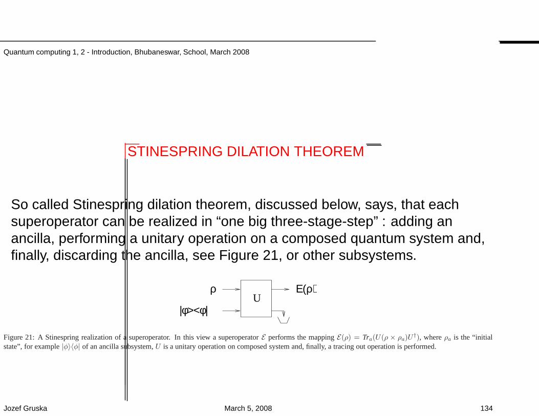
Quantum computing 1, 2 - Introduction, Bhubaneswar, School, March 2008
STINESPRING DILATION THEOREM
So called Stinespring dilation theorem, discussed below, says, that eachsuperoperator can be realized in “one big three-stage-step” : adding anancilla, performing a unitary operation on a composed quantum system and,finally, discarding the ancilla, see Figure 21, or other subsystems.
ρ
|φ><φ|
Ε(ρ)U
Figure 21: A Stinespring realization of a superoperator. Inthis view a superoperatorE performs the mappingE(ρ) = Tra(U(ρ × ρa)U†), whereρa is the “initial
state”, for example|φ〉〈φ| of an ancilla subsystem,U is a unitary operation on composed system and, finally, a tracing out operation is performed.
Jozef Gruska March 5, 2008 134
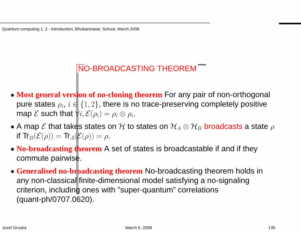
Quantum computing 1, 2 - Introduction, Bhubaneswar, School, March 2008
NO-BROADCASTING THEOREM
• Most general version of no-cloning theoremFor any pair of non-orthogonalpure states ρi, i ∈ 1, 2, there is no trace-preserving completely positivemap E such that ∀i,E(ρi) = ρi ⊗ ρi.• A map E that takes states on H to states on HA ⊗HB broadcasts a state ρ
if TrB(E(ρ)) = TrA(E(ρ)) = ρ.
• No-broadcasting theoremA set of states is broadcastable if and if theycommute pairwise.
• Generalised no-broadcasting theoremNo-broadcasting theorem holds inany non-classical finite-dimensional model satisfying a no-signalingcriterion, including ones with ”super-quantum” correlations(quant-ph/0707.0620).
Jozef Gruska March 5, 2008 135
Quantum computing 1, 2 - Introduction, Bhubaneswar, School, March 2008
QUANTUM ERROR CORRECTION I
In the quantum case, information processing evolutions are far more underthe negative impact of their environment, called in general decoherence,than in the classical computing.
The impact of decoherence is actually in all known technologies so strong,and grows exponentially in time, that till 1995 there have been strong doubtswhether a powerful quantum information processing is possible at all.
A strong reason for pessimism was a belief (understanding) that in thequantum case one cannot use some quantum modification of so powerfulclassical error-correcting code approach.
There were several physical reasons for such a pessimism.
One of them was that in order to determine an error, we would need tomeasure the erroneous state, but that would irreversibly modify/destroy theerroneous state and we would have nothing to correct. Fortunately, it hasturned out that there is a way out and quantum error correction can workwell. The example presented in this section demonstrates the basic stepshow such an error correction process can work, in principle.
Jozef Gruska March 5, 2008 136
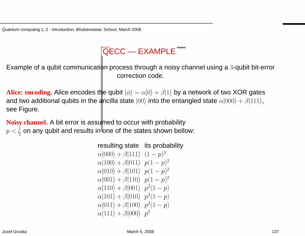
Quantum computing 1, 2 - Introduction, Bhubaneswar, School, March 2008
QECC — EXAMPLE
Example of a qubit communication process through a noisy channel using a 3-qubit bit-errorcorrection code.
Alice: encoding.Alice encodes the qubit |φ〉 = α|0〉 + β|1〉 by a network of two XOR gatesand two additional qubits in the ancilla state |00〉 into the entangled state α|000〉 + β|111〉,see Figure.
Noisy channel.A bit error is assumed to occur with probabilityp < 1
2on any qubit and results in one of the states shown bellow:
resulting state its probabilityα|000〉 + β|111〉 (1− p)3α|100〉 + β|011〉 p(1− p)2α|010〉 + β|101〉 p(1− p)2α|001〉 + β|110〉 p(1− p)2α|110〉 + β|001〉 p2(1− p)α|101〉 + β|010〉 p2(1− p)α|011〉 + β|100〉 p2(1− p)α|111〉 + β|000〉 p3
Jozef Gruska March 5, 2008 137
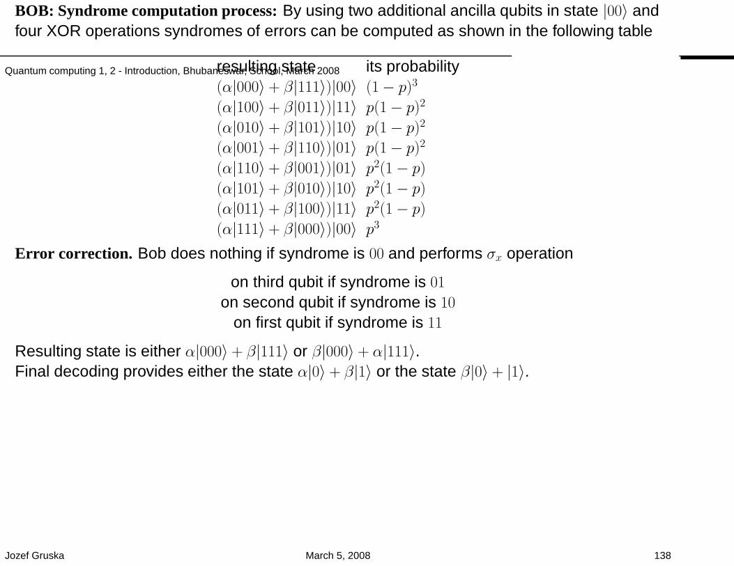
Quantum computing 1, 2 - Introduction, Bhubaneswar, School, March 2008
BOB: Syndrome computation process:By using two additional ancilla qubits in state |00〉 andfour XOR operations syndromes of errors can be computed as shown in the following table
resulting state its probability(α|000〉 + β|111〉)|00〉 (1− p)3(α|100〉 + β|011〉)|11〉 p(1− p)2(α|010〉 + β|101〉)|10〉 p(1− p)2(α|001〉 + β|110〉)|01〉 p(1− p)2(α|110〉 + β|001〉)|01〉 p2(1− p)(α|101〉 + β|010〉)|10〉 p2(1− p)(α|011〉 + β|100〉)|11〉 p2(1− p)(α|111〉 + β|000〉)|00〉 p3
Error correction. Bob does nothing if syndrome is 00 and performs σx operation
on third qubit if syndrome is 01
on second qubit if syndrome is 10
on first qubit if syndrome is 11
Resulting state is either α|000〉 + β|111〉 or β|000〉 + α|111〉.Final decoding provides either the state α|0〉 + β|1〉 or the state β|0〉 + |1〉.
Jozef Gruska March 5, 2008 138
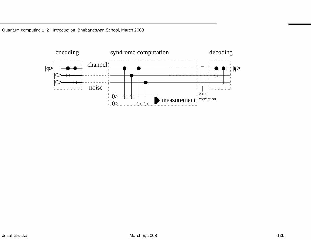
Quantum computing 1, 2 - Introduction, Bhubaneswar, School, March 2008
errorcorrection
|0>|0>
|φ>
encoding
channel
noise|0>|0> measurement
syndrome computation decoding
|φ>
Jozef Gruska March 5, 2008 139
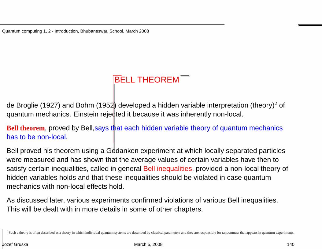
Quantum computing 1, 2 - Introduction, Bhubaneswar, School, March 2008
BELL THEOREM
de Broglie (1927) and Bohm (1952) developed a hidden variable interpretation (theory)2 ofquantum mechanics. Einstein rejected it because it was inherently non-local.
Bell theorem, proved by Bell,says that each hidden variable theory of quantum mechanicshas to be non-local.
Bell proved his theorem using a Gedanken experiment at which locally separated particleswere measured and has shown that the average values of certain variables have then tosatisfy certain inequalities, called in general Bell inequalities, provided a non-local theory ofhidden variables holds and that these inequalities should be violated in case quantummechanics with non-local effects hold.
As discussed later, various experiments confirmed violations of various Bell inequalities.This will be dealt with in more details in some of other chapters.
2Such a theory is often described as a theory in which individual quantum systems are described by classical parameters and they are responsible for randomness that appears in quantum experiments.
Jozef Gruska March 5, 2008 140
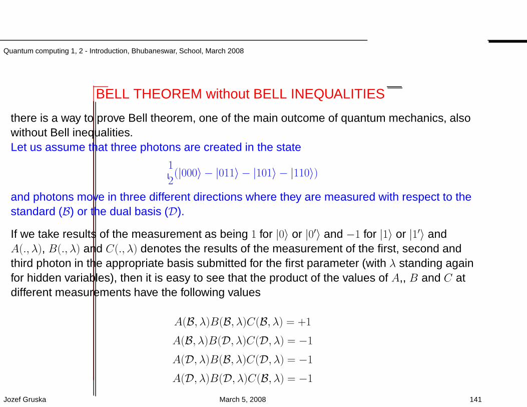
Quantum computing 1, 2 - Introduction, Bhubaneswar, School, March 2008
BELL THEOREM without BELL INEQUALITIES
there is a way to prove Bell theorem, one of the main outcome of quantum mechanics, alsowithout Bell inequalities.Let us assume that three photons are created in the state
1
2(|000〉 − |011〉 − |101〉 − |110〉)
and photons move in three different directions where they are measured with respect to thestandard (B) or the dual basis (D).
If we take results of the measurement as being 1 for |0〉 or |0′〉 and −1 for |1〉 or |1′〉 andA(., λ), B(., λ) and C(., λ) denotes the results of the measurement of the first, second andthird photon in the appropriate basis submitted for the first parameter (with λ standing againfor hidden variables), then it is easy to see that the product of the values of A,, B and C atdifferent measurements have the following values
A(B, λ)B(B, λ)C(B, λ) = +1
A(B, λ)B(D, λ)C(D, λ) = −1
A(D, λ)B(B, λ)C(D, λ) = −1
A(D, λ)B(D, λ)C(B, λ) = −1
Jozef Gruska March 5, 2008 141
Quantum computing 1, 2 - Introduction, Bhubaneswar, School, March 2008
In the case there are no non-local influences the result of one measurement cannotinfluence the other two and therefore we can assume that values of variables A,B and Cappearing in different equations for the same basis are the same. We can then multiply theleft and the right sides of all four equalities. However, the product of the left sides gives thevalue 1 because each value appears there twice and the product of the right sides gives thevalue −1. A contradiction.
Jozef Gruska March 5, 2008 142
Quantum computing 1, 2 - Introduction, Bhubaneswar, School, March 2008
IS THE WORLD CLASSICAL?
The notion of the classical world includes mainly two ingredients: (a)realism; (b) determinism.
By realism we mean that any quantity that can be measured is well definedeven if we do not measure it in practice.
By determinism we mean that that the result of a measurement isdetermined in a definite way by the state of the system and by themeasurement setup.
Quantum world does not satisfy the above two requirements.
A particle in the state |0′〉 has no definite value with respect to measurementwith respect to the standard basis - realism does not take place.
Measurement of a particle in state 0′〉 with respect to the standard basisprovides with the same probability results 0 and 1 - determinism does nottake place.
Jozef Gruska March 5, 2008 143
Quantum computing 1, 2 - Introduction, Bhubaneswar, School, March 2008
CLASSICAL versus QUANTUM WORLDS
• The border between classical and quantum phenomena is justa question of money. (A. Zeilinger)
• The classical-quantum boundary is simply a matter ofinformation control. (M. Aspelmeyer)
• There is no border between classical and quantumphenomena – you just have to look closer. (R. Bertlman)
• There is no classical world - there is only quantum world (D.Greenberger).
• There is no quantum world. There is only an abstractquantum physical description. It is wrong to think that the taskof physics is to find out how Nature is. Physics concerns whatwe c an say about Nature. (N. Bohr)
Jozef Gruska March 5, 2008 144
Quantum computing 1, 2 - Introduction, Bhubaneswar, School, March 2008
CLASSICAL versus QUANTUM PHYSICS
I believe there is no classical world. There is only quantumworld.
Classical physics is a collection of unrelated insights: Newton’slaws. Hamilton’s principle, etc. Only quantum theory brings outtheir connection.
An analogy is the Hawaiian Islands, which look like a bunch ofisland in the ocean. But if you could lower the water, you wouldsee, that they are the peaks of a chain of mountains.
That is what quantum physics does to classical physics.D. Greenberger
Jozef Gruska March 5, 2008 145
Quantum computing 1, 2 - Introduction, Bhubaneswar, School, March 2008
UNFINISHED REVOLUTION
• Some consider Einstein’s revolution as unfinished because itdoes not provide a unified view of quantum world withspace-time.
• Basic question: is quantum theory correct or it needs to bemodified before it can be unified with our understanding oftime and space.
Jozef Gruska March 5, 2008 146
Quantum computing 1, 2 - Introduction, Bhubaneswar, School, March 2008
UNSCRAMBLING of OMELET
Today we are beginning to realize how much of all physical science is reallyonly information, organized in a particular way.
But we are far from unraveling the knotty question: To what extent does thisinformation reside in us, and to what extent is it a property of nature?
Our present quantum mechanics formalism is a peculiar mixture describingin part laws of Nature, in part incomplete human information about Nature –all scrambled up together by Bohr into an omelet that nobody has seen howto unscramble,
Yet we think the unscrambling is a prerequisite for any further advances inbasic physical theory. .. Edwin T. Jaynes, 1990
Jozef Gruska March 5, 2008 147
Quantum computing 1, 2 - Introduction, Bhubaneswar, School, March 2008
KEY QUESTIONS and/or STEPS in the DEVELOPMENT of QIPC
Key steps in the development of QIPC were separations of four problems:
P1Can we build powerful quantum computers?
P2What could be achieved with powerful quantum computers?
P3What are the laws and limitations of quantum informationprocessing and communication?
P4Can we develop a better understanding of the quantum worldon the basis of the laws and limitations of QIPC?
This separation allowed complexity theory to make substantial contributions to the attemptsto solve problems P2 and P3, especially P2, and to set as its new goal a contribution to thesolution of the problem P4.
New recent goal and challenge of complexity theory is to helpto deal with the problem P1.
Jozef Gruska March 5, 2008 148
Quantum computing 1, 2 - Introduction, Bhubaneswar, School, March 2008
WHAT IS QUANTUM INFORMATION?
The views on what is quantum information differ.
• There is no quantum information, there are only quantumcarriers of classical information. (A. Zeilinger).
• Concept of quantum information is primary fundamentalconcept/ingredient of quantum physics that cannot be defined.However, the viewpoint it suggest is richly suggestive, leadingto new interesting questions and interpretations of quantumprocesses. (J. Jozsa)
Jozef Gruska March 5, 2008 149
Quantum computing 1, 2 - Introduction, Bhubaneswar, School, March 2008
STARTING/CLOSING VIEWS
• Nothing exists except atoms and empty space; everythingelse is opinion. Democritus of Abdera (ca. 400 BC).
• In science there is only Physics: all the rest is stampcollecting. Ernest Rutherford (1912)
Jozef Gruska March 5, 2008 150
Quantum computing 1, 2 - Introduction, Bhubaneswar, School, March 2008
CHANGING WORLD
Views on the role of physics in the understanding of the physicalworld keep developing.
• Nothing exists except atoms and empty space; everything else isopinion. Democritus of Abdera (ca. 400 BC).
• In Science there is only Physics: all the rest is stamps collecting.Ernest Rutherford (1912)
• Physics is like sex; it produces sometimes practical results, butthis is not reason why we do it. Feynman (19??)
• Physics is not the only science to get deep understanding ofphysical world. Informatics can and should help. Or, even, itshould take an initiative?
Jozef Gruska March 5, 2008 151
Quantum computing 1, 2 - Introduction, Bhubaneswar, School, March 2008
THERE IS A NEED TO CHANGE EMPHASES IN
QUANTUM INFORMATION PROCESSING
from
QUANTUM INFORMATION PRECESSING
to
CLASSICAL/QUANTUM INFORMATION PROCESSING
Jozef Gruska March 5, 2008 152
Quantum computing 1, 2 - Introduction, Bhubaneswar, School, March 2008
ANOTHER CLOSING MOTTO
Sorry, I am not young enough to know everything.
Jozef Gruska March 5, 2008 153
QUANTUM INFORMATION PROCESSING PRIMITIVESAND THEIR OPTIMAL USE
Jozef Gruska
Faculty of Informatics, Brno, Czech Republik
March 5, 2008
Quantum computing 3 - Quantum computation primitives - Bhubaneswar, March, 2008
ABSTRACT
This talk deals with several concepts of universality in quantuminformation processing and with various (sometimes surprising)universal sets of (often surprising) quantum primitives.
In the talk we also deal with recent developments concerningan optimal use of some quantum primitives.
Jozef Gruska March 5, 2008 1

Quantum computing 3 - Quantum computation primitives - Bhubaneswar, March, 2008
PART I - MOTIVATION
Jozef Gruska March 5, 2008 2
Quantum computing 3 - Quantum computation primitives - Bhubaneswar, March, 2008
MOTTO I.
Progress in science is often done by pessimists.Progress in technology is always done by optimists.
Jozef Gruska March 5, 2008 3
Quantum computing 3 - Quantum computation primitives - Bhubaneswar, March, 2008
MOTTO II.
Progress in science is often done by pessimists.Progress in technology is always done by knowledgeable and
experienced optimists.
Jozef Gruska March 5, 2008 4
Quantum computing 3 - Quantum computation primitives - Bhubaneswar, March, 2008
TWO STORIES TO REMEMBER
• The proposal to build Collosus, the first electronic computer forcryptanalysis purposes, was during 2WW rejected by a committee ofprominent specialists as impossible to make, in spite of the fact that Britishcryptanalysts needed it badly to crack communication between Hitler andhis generals.
• Collosus was then built by an ingenious optimist, Tommy Flowers, within10 months in a Post office laboratory, and worked from the beginningsuccessfully to break Lorenz cipher, starting January 1944.
• The key point was that Flowers realized that velvets were reliable providedthey were never switched on and off. (Of course, nobody believed him.)
• The idea that 30m long ENIAC with 19000 vacuum tubes could worklooked also crazy, for scientists, but it worked.
Jozef Gruska March 5, 2008 5
Quantum computing 3 - Quantum computation primitives - Bhubaneswar, March, 2008
TRY TO BELIEVE IMPOSSIBLE
There’s no use in trying, she said: one can’t believe impossiblethings
I daresay you haven’t had much practice said the Queen.
When I was your age, I always did it for half-an-hour a day.
Why sometimes I’ve believed as many as six impossible thingsbefore breakfast.
Lewis Carol: Through the Looking-glass, 1872
Jozef Gruska March 5, 2008 6
Quantum computing 3 - Quantum computation primitives - Bhubaneswar, March, 2008
REALITY and PERSPECTIVES
• Factoring of the number 15 has been so far the most publicized outcome ofexperimental quantum computing (not to mention excellent cryptography,superposition, entanglement and teleportation experiments).
• DARPA set up as goal, in 2004 in the FoQuS program, to built a quantum processor tofactorize 128 bit numbers in less than 30 seconds and with 99.99% accuracy.
• DARPA Quantum Cryptography Network operates in Cambridge, USA, connecting allcampuses of Boston and Harvard University, and operates non-stop.
• Hundred qubits processors “are on the drawing table now (Steane (2005) has recentlytried to justify that 300 qubit processors with laser controlled trap ion is feasible;Chuang et al. see possible to factorize 1024 numbers in 31 hours (classically it wouldrequire billion times longer than to factorize 512-bit numbers what required, in 2000,8400 MIPS years).
• Emerging quantum technologies promise even larger scalability.
Jozef Gruska March 5, 2008 7
Quantum computing 3 - Quantum computation primitives - Bhubaneswar, March, 2008
BASIC OBSERVATIONS – I
• Nature offers many ways – let us call them technologies – various quantum informationprocessing primitives can be exhibited, realized and utilized.
• Since it appears to be very difficult to exploit potential of nature for QIP, it is of largeimportance to explore which quantum primitives form universal sets of primitives, and are(quite) easy to implement.
• Also from the point of view of understanding of the laws and limitations of QIP and also ofquantum mechanics itself, the problems of finding rudimentary and universal QIPprimitives , as well as methods for their optimal use, are of large experimental andfundamental importance.
• Search for quantum computation universal primitives, and their optimal use, is actuallyone of the major tasks of the current QIP research (both theoretical and experimental)that starts to attack the task of building quantum processors seriously.
• The search for sets of elementary, or even very rudimentary, but powerful, quantumcomputational primitives and for their optimal use, has brought a variety of deep andsurprising results that seem to be also much encouraging for experimentalists.
Jozef Gruska March 5, 2008 8
Quantum computing 3 - Quantum computation primitives - Bhubaneswar, March, 2008
BASIC OBSERVATIONS – II
Observation: An apparently small observation of a scientists oran experience of an engineer can turn a field upside down and“create a superstar from a sleeping beauty”.
Conclusion: It is very, very important to search for primitivesand for new and new primitives - even in the areas one canhardly expect them.
Jozef Gruska March 5, 2008 9
Quantum computing 3 - Quantum computation primitives - Bhubaneswar, March, 2008
BASIC QUESTIONS
• How to decide which primitives are of importance?
• Where to find “precedence” for such a decision?
Jozef Gruska March 5, 2008 10
Quantum computing 3 - Quantum computation primitives - Bhubaneswar, March, 2008
TWO NATURAL QUESTIONS?
• What are the main reason that classical computing has beenso successful?
• What can quantum computing learn from the classicalcomputing success story?
Jozef Gruska March 5, 2008 11
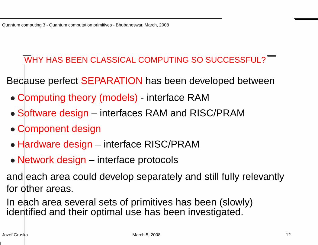
Quantum computing 3 - Quantum computation primitives - Bhubaneswar, March, 2008
WHY HAS BEEN CLASSICAL COMPUTING SO SUCCESSFUL?
Because perfect SEPARATION has been developed between
• Computing theory (models) - interface RAM
• Software design – interfaces RAM and RISC/PRAM
• Component design
• Hardware design – interface RISC/PRAM
• Network design – interface protocols
and each area could develop separately and still fully relevantlyfor other areas.In each area several sets of primitives has been (slowly)identified and their optimal use has been investigated.
Jozef Gruska March 5, 2008 12
Quantum computing 3 - Quantum computation primitives - Bhubaneswar, March, 2008
AN OBSERVATION
We need to find proper sets of primitives for quantuminformation processing.
Jozef Gruska March 5, 2008 13
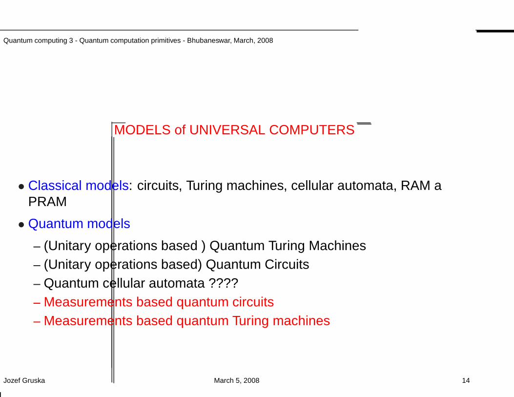
Quantum computing 3 - Quantum computation primitives - Bhubaneswar, March, 2008
MODELS of UNIVERSAL COMPUTERS
• Classical models: circuits, Turing machines, cellular automata, RAM aPRAM
• Quantum models
– (Unitary operations based ) Quantum Turing Machines– (Unitary operations based) Quantum Circuits– Quantum cellular automata ????– Measurements based quantum circuits– Measurements based quantum Turing machines
Jozef Gruska March 5, 2008 14
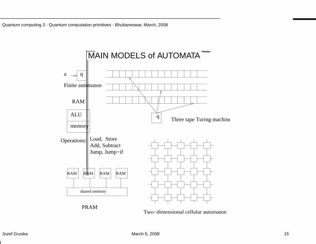
Quantum computing 3 - Quantum computation primitives - Bhubaneswar, March, 2008
MAIN MODELS of AUTOMATA
a q
qALU
memory
Operations:Load, StoreAdd, SubtractJump, Jump−if
RAM
Three tape Turing machine
Two−dimensional cellular automaton
RAM RAM RAM RAM
shared memory
PRAM
Finite automaton
Jozef Gruska March 5, 2008 15
Quantum computing 3 - Quantum computation primitives - Bhubaneswar, March, 2008
INSIGHTS into QIPC
• BASIC TASKS of QUANTUM COMPUTER DESIGN
– To find ways to set up initial state
– To find ways to implement a universal sets of quantum gates
– To realize ways to implement quantum circuits
– To find ways to perform quantum measurements
• BASIC TASKS of (UNITARY-BASED) QUANTUM COMPUTATIONS
– To set up an initial state
– To make quantum system to implement unitary gates of a quantum circuit.
– To perform measurements to get outcome
• NEW (MEASUREMENT-BASED) VIEW of QUANTUM COMPUTATIONS
Measurement is the basic way to force closed quantum systems to do what we want it todo (to perform unitaries) in order to solve (classical) computation problems.
Jozef Gruska March 5, 2008 16
Quantum computing 3 - Quantum computation primitives - Bhubaneswar, March, 2008
KEY STEPS in DEVELOPMENT of QIPC
Key steps in the development of QIPC were separations of four problems:
P1 Can we build (and how) powerful quantum computers?
P2 What could be achieved with powerful quantum computers?
P3 What are the laws and limitations of quantum information processing andcommunication?
P4 Can we develop a better understanding of the quantum world on the basisof the laws and limitations of QIPC?
This separation allowed complexity theory to make substantial contributions to the attemptsto solve problems P2 and P3, especially P2, and to set as its new goal a contribution to thesolution of the problem P4.
New recent goal and challenge of complexity theory is to help to answer theproblem P1.
Jozef Gruska March 5, 2008 17
Quantum computing 3 - Quantum computation primitives - Bhubaneswar, March, 2008
SETS of UNIVERSAL PRIMITIVES in CLASSICAL COMPUTING
• In classical computing, the most often used universal sets of gates are
– AND-, OR- and NOT-gates,– AND- and NOT-gates,– NOR- (NAND-) or [AOI]-gate (that require few CMOS transistors)
• The optimization problem for classical circuits with such sets of gates hasbeen solved quite satisfactorily.
• In case of classical reversible computing, universal are both the Toffoli gate
T (x, y, z) = (x, y, (x ∧ y) ⊕ z)
and the Fredkin gate
F (x, y, z) = (x, xy + xz, xz + xy),
if constant inputs are allowed, as well as “wires” with the identity gates.
Jozef Gruska March 5, 2008 18
Quantum computing 3 - Quantum computation primitives - Bhubaneswar, March, 2008
WHY REVERSIBLE CLASSICAL CIRCUITS?
Reversible classical circuits started to be of increased importance recently for several
reasons:
• They are of importance in some applications, as signal processing,communication, cryptography, where circuits should be informationlossless;
• Reversibility is of importance for some technologies where the loss ofinformation due to irreversibility implies energy losses.
• Reversibility is of importance for some nanotechnologies, where switchingdevises with gain are not easy to construct;
• Reversible classical circuits are special cases of quantum circuits.
Jozef Gruska March 5, 2008 19
Quantum computing 3 - Quantum computation primitives - Bhubaneswar, March, 2008
UNIVERSALITY of SETS of CLASSICAL REVERSIBLE GATES
Definition 0.1 A set of reversible gates G is universal if for every n there existsa constant cn such that for any permutation π ∈ S2n there exists a G-circuitwhich computes π using cn ancilla wires.
• Toffoli (1980) has shown that an = n− 3 in case the set of gates
CNT = CNOT, NOT, TOFFOLI is used.
• Shende et al. (2002) have shown for circuits implementing even (odd)permutations that cn = 0 (cn = 1) in case of the set CNT.
Jozef Gruska March 5, 2008 20
Quantum computing 3 - Quantum computation primitives - Bhubaneswar, March, 2008
OPTIMIZATION METHODS
Optimization of reversible circuits concerns the following characteristics: number of ancillas,number of gates and depth of the circuit.
• Optimization problem (concerning number of gates) for an important class ofCNOT-circuits has been solved by K. N. Patel et al. (2002).
• The basic observation is that each circuit consisting of CNOT-gates realizes a so calledxor-linear gate and vice verse.
• An n qubit gate U is called xor-linear if U(x⊕ y) = U(x) ⊕ U(y) holds for everyx, y ∈ 0, 1n.
• They provide an algorithm that implements any xor-linear n qubit gate using O(n2/lgn)
CNOT-gates and they also showed that this result is asymptotically optimal.
• Optimization of CNOT,NOT circuits has been solved by Iwama and Yamashita (2003).They found a complete set of transformation rules that can transform anyCNOT,NOT-circuit to an optimal one. However, time complexity of optimization isexponential.
Jozef Gruska March 5, 2008 21
Quantum computing 3 - Quantum computation primitives - Bhubaneswar, March, 2008
MINIMIZATION of the NUMBER of TOFFOLI GATES
Toffoli gates are, in a sense, strongest classical reversible gates. Ofimportance and interest is therefore the following problem.
Given a reversible function f(x), what is the minimum number of Toffoligates needed to construct a circuit that will evaluate f(x) for every x.
By Popescu et al. (04070350) there are reversible functions for whichnumber of Toffoli gates grows exponentially.
Popescu et al. (0407035) have shown that given a classical reversiblefunction f , one can construct a unitary transformation Uf such that if Uf is“non-local”, then f cannot be realized by a reversible circuit with two-bitgates only and the amount of non-locality of Uf provides a lower bound onthe number of Toffoli gates needed.
The amount of non-locality of a gate U , denoted EU , is defined as theminimum amount of entanglement, in ebits, which allows to implement Uusing LOCC.
Jozef Gruska March 5, 2008 22
Quantum computing 3 - Quantum computation primitives - Bhubaneswar, March, 2008
LOWER BOUNDS on the number of TOFFOLI GATES
It holdsTU ≥ EU
ETof
where TU is number of Toffoli gates to implement U .
Popescu et al (0407035) have shown methods how to determine lowerbound EU and determined ETof .
This has been again an example that inherently quantum tools have beenused to solve a classical problem.
Jozef Gruska March 5, 2008 23
Quantum computing 3 - Quantum computation primitives - Bhubaneswar, March, 2008
QUANTUM PRIMITIVES
Jozef Gruska March 5, 2008 24
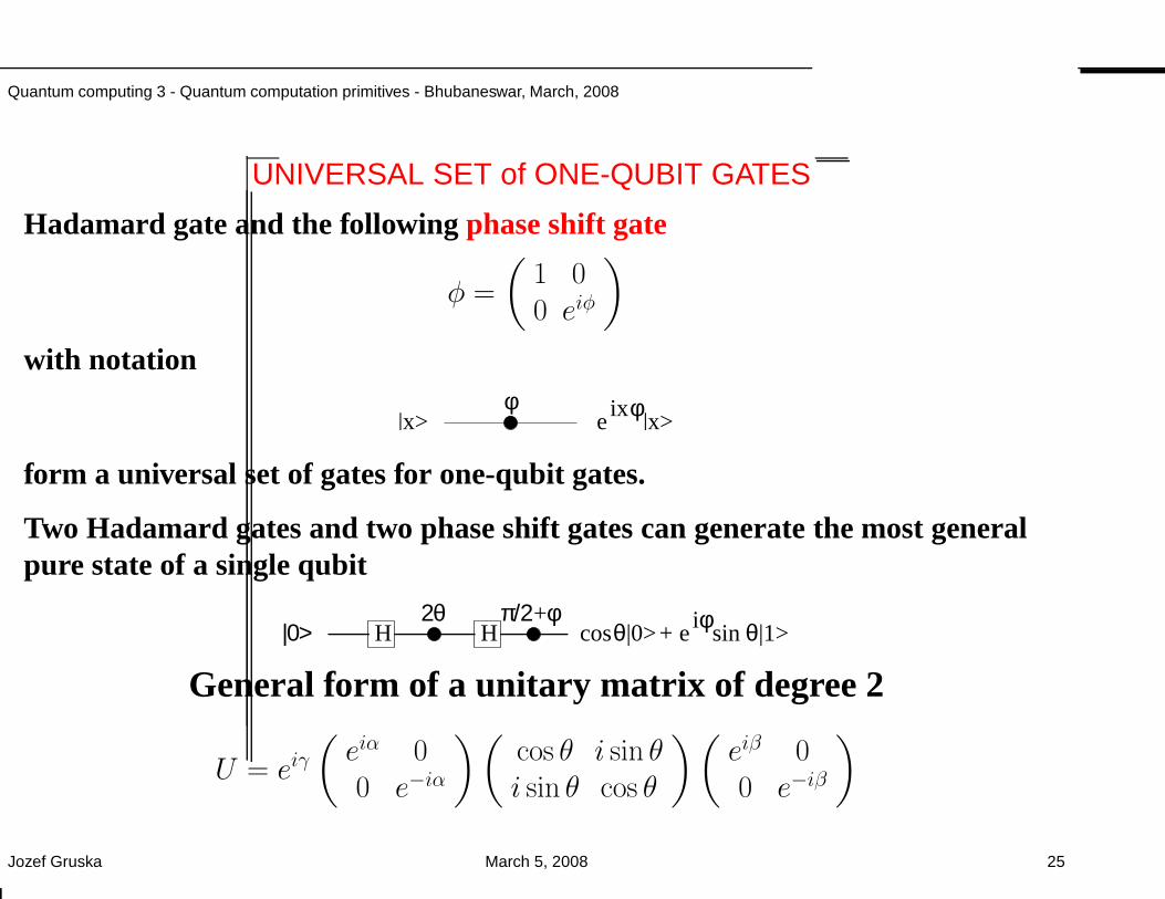
Quantum computing 3 - Quantum computation primitives - Bhubaneswar, March, 2008
UNIVERSAL SET of ONE-QUBIT GATES
Hadamard gate and the followingphase shift gate
φ =
(
1 00 eiφ
)
with notation
|x>φ
eixφ|x>
form a universal set of gates for one-qubit gates.
Two Hadamard gates and two phase shift gates can generate themost generalpure state of a single qubit
|0> HH2θ p/2+φ
cosθ|0>+ eiφsinθ|1>
General form of a unitary matrix of degree 2
U = eiγ(
eiα 00 e−iα
)(
cos θ i sin θi sin θ cos θ
)(
eiβ 00 e−iβ
)
Jozef Gruska March 5, 2008 25
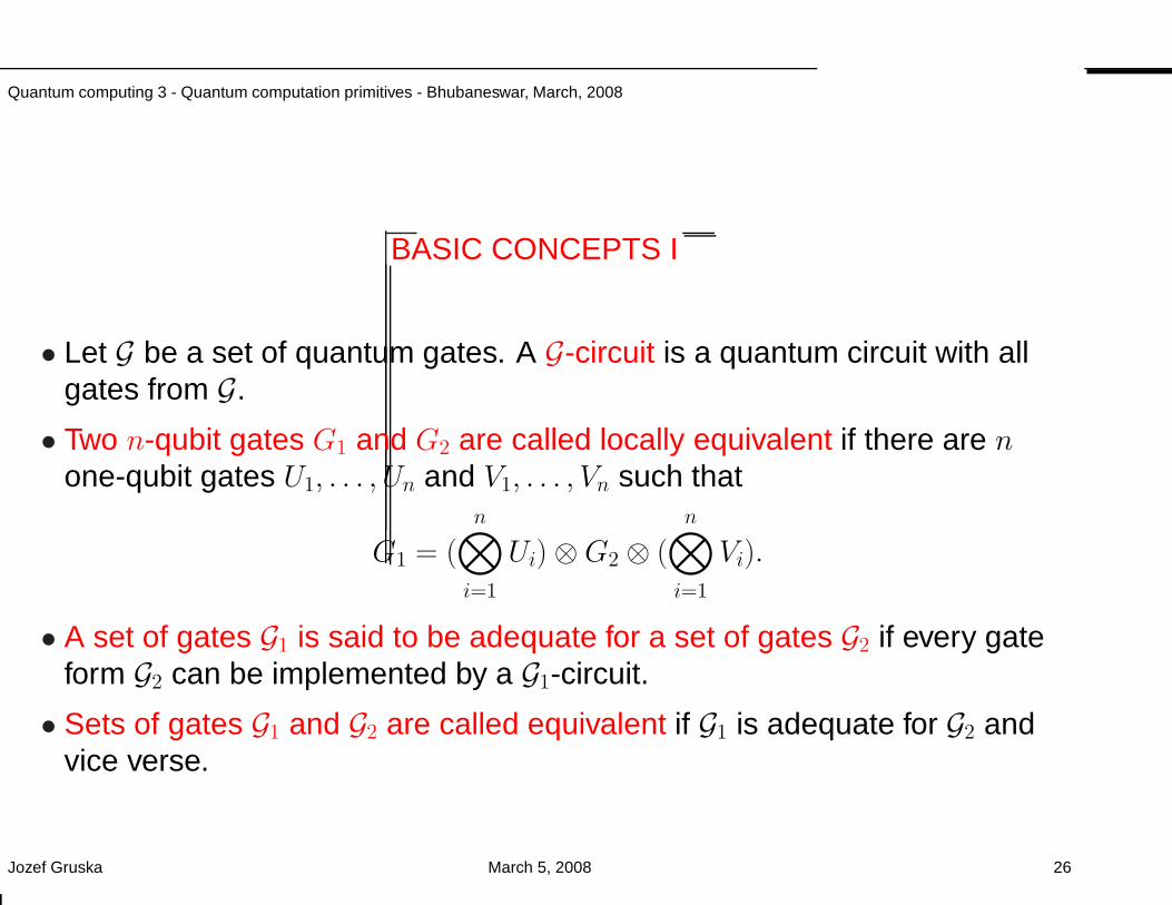
Quantum computing 3 - Quantum computation primitives - Bhubaneswar, March, 2008
BASIC CONCEPTS I
• Let G be a set of quantum gates. A G-circuit is a quantum circuit with allgates from G.
• Two n-qubit gates G1 and G2 are called locally equivalent if there are none-qubit gates U1, . . . , Un and V1, . . . , Vn such that
G1 = (n⊗
i=1
Ui) ⊗G2 ⊗ (n⊗
i=1
Vi).
• A set of gates G1 is said to be adequate for a set of gates G2 if every gateform G2 can be implemented by a G1-circuit.
• Sets of gates G1 and G2 are called equivalent if G1 is adequate for G2 andvice verse.
Jozef Gruska March 5, 2008 26
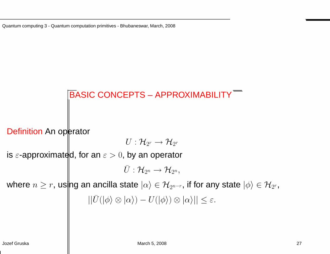
Quantum computing 3 - Quantum computation primitives - Bhubaneswar, March, 2008
BASIC CONCEPTS – APPROXIMABILITY
Definition An operatorU : H2r → H2r
is ε-approximated, for an ε > 0, by an operator
U : H2n → H2n,
where n ≥ r, using an ancilla state |α〉 ∈ H2n−r, if for any state |φ〉 ∈ H2r,
||U(|φ〉 ⊗ |α〉) − U (|φ〉) ⊗ |α〉|| ≤ ε.
Jozef Gruska March 5, 2008 27
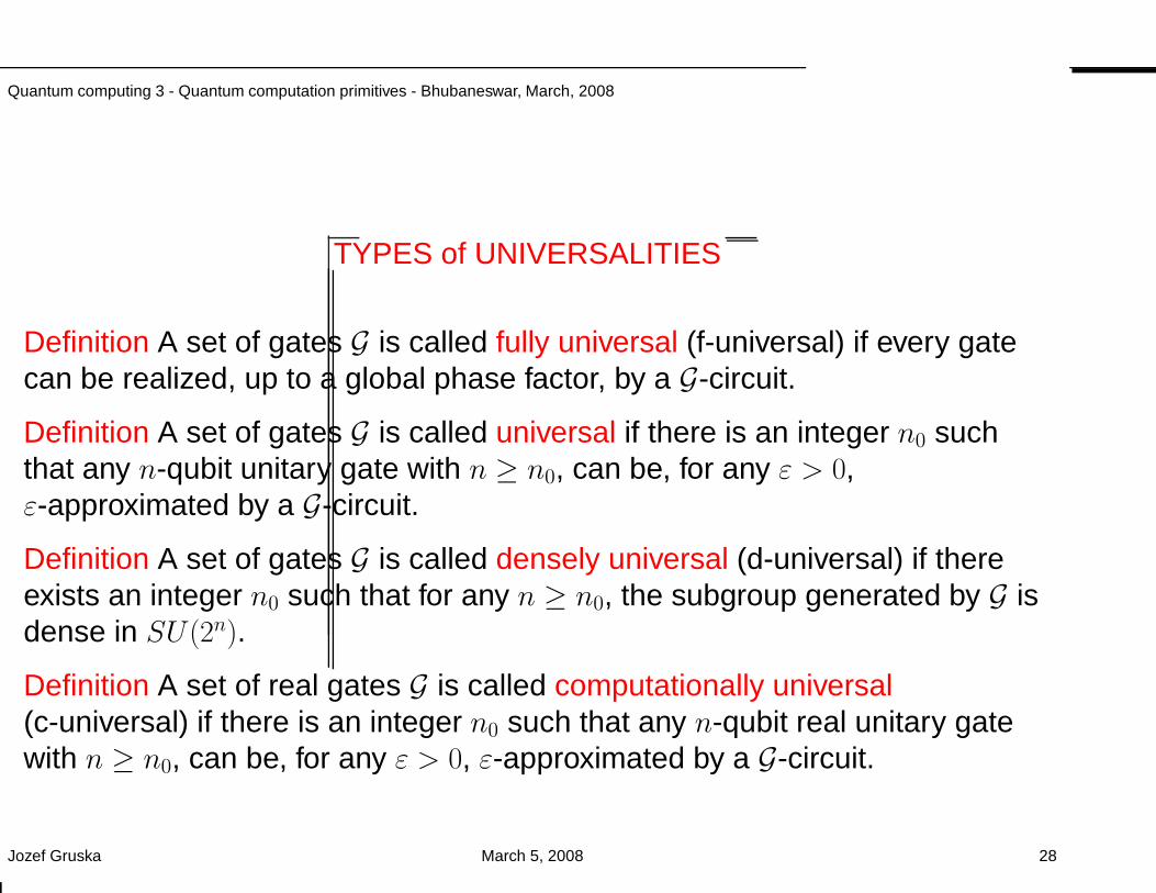
Quantum computing 3 - Quantum computation primitives - Bhubaneswar, March, 2008
TYPES of UNIVERSALITIES
Definition A set of gates G is called fully universal (f-universal) if every gatecan be realized, up to a global phase factor, by a G-circuit.
Definition A set of gates G is called universal if there is an integer n0 suchthat any n-qubit unitary gate with n ≥ n0, can be, for any ε > 0,ε-approximated by a G-circuit.
Definition A set of gates G is called densely universal (d-universal) if thereexists an integer n0 such that for any n ≥ n0, the subgroup generated by G isdense in SU (2n).
Definition A set of real gates G is called computationally universal(c-universal) if there is an integer n0 such that any n-qubit real unitary gatewith n ≥ n0, can be, for any ε > 0, ε-approximated by a G-circuit.
Jozef Gruska March 5, 2008 28
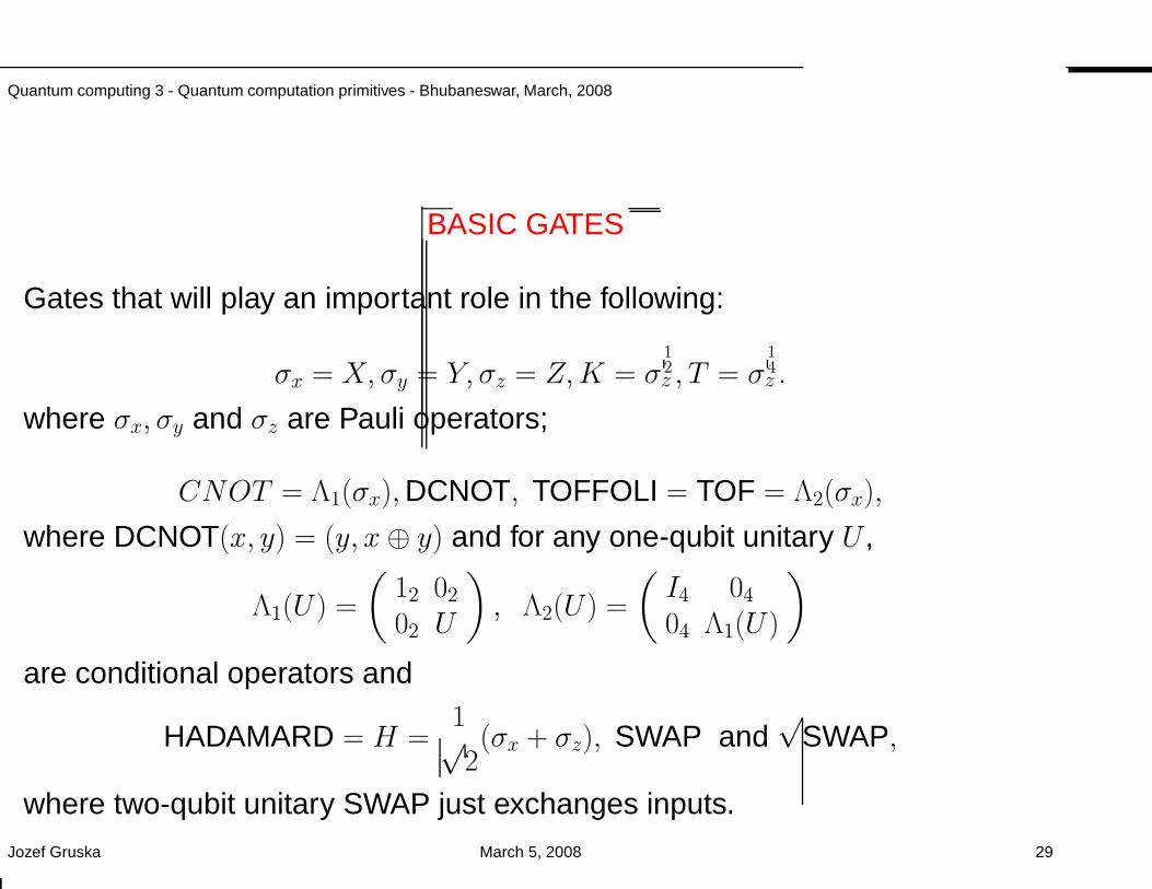
Quantum computing 3 - Quantum computation primitives - Bhubaneswar, March, 2008
BASIC GATES
Gates that will play an important role in the following:
σx = X, σy = Y, σz = Z,K = σ12z , T = σ
14z .
where σx, σy and σz are Pauli operators;
CNOT = Λ1(σx),DCNOT, TOFFOLI = TOF = Λ2(σx),
where DCNOT(x, y) = (y, x⊕ y) and for any one-qubit unitary U ,
Λ1(U ) =
(
12 02
02 U
)
, Λ2(U ) =
(
I4 04
04 Λ1(U )
)
are conditional operators and
HADAMARD = H =1√2(σx + σz), SWAP and
√SWAP,
where two-qubit unitary SWAP just exchanges inputs.
Jozef Gruska March 5, 2008 29
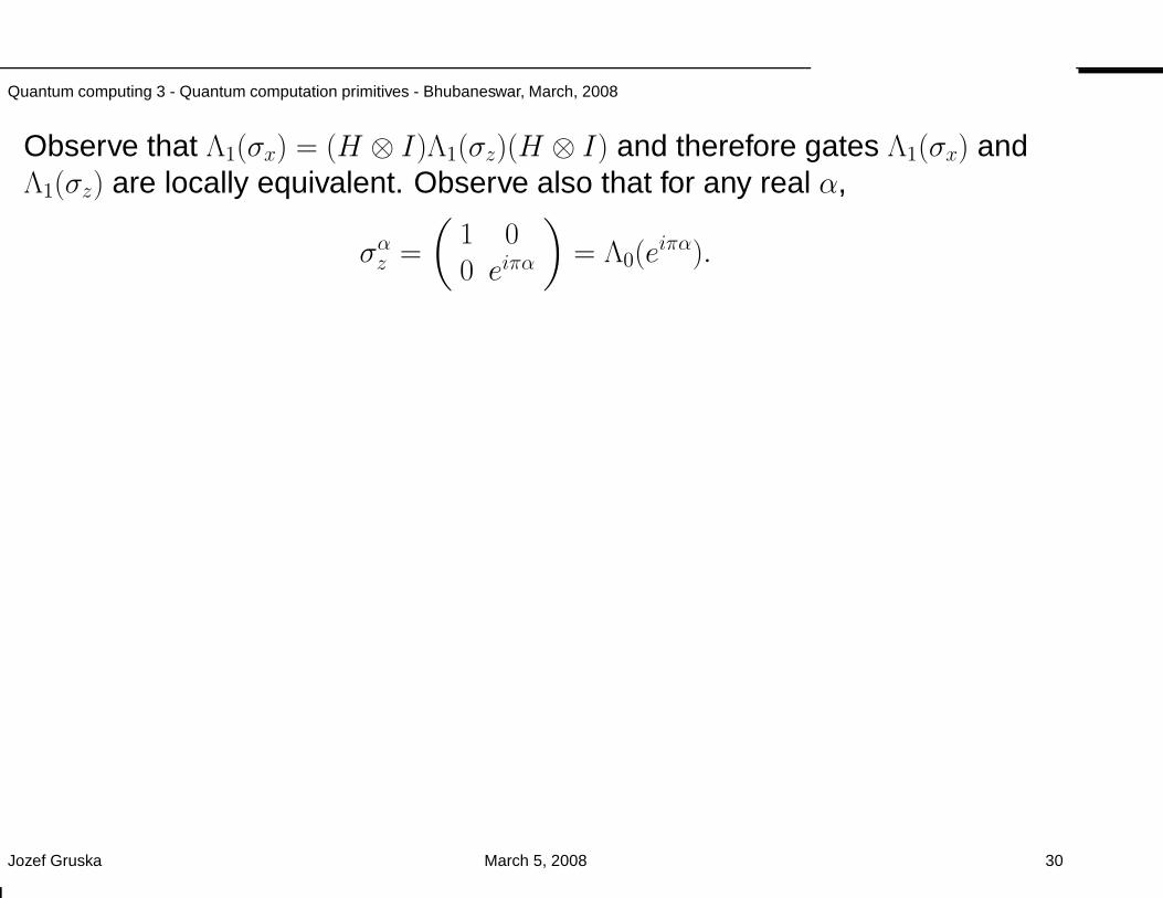
Quantum computing 3 - Quantum computation primitives - Bhubaneswar, March, 2008
Observe that Λ1(σx) = (H ⊗ I)Λ1(σz)(H ⊗ I) and therefore gates Λ1(σx) andΛ1(σz) are locally equivalent. Observe also that for any real α,
σαz =
(
1 00 eiπα
)
= Λ0(eiπα).
Jozef Gruska March 5, 2008 30
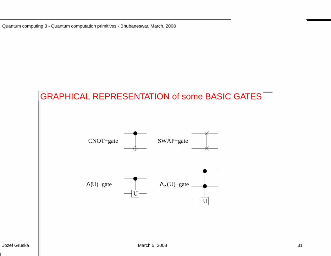
Quantum computing 3 - Quantum computation primitives - Bhubaneswar, March, 2008
GRAPHICAL REPRESENTATION of some BASIC GATES
CNOT−gate SWAP−gate
UU
L(U)−gate L (2 U)−gate
Jozef Gruska March 5, 2008 31
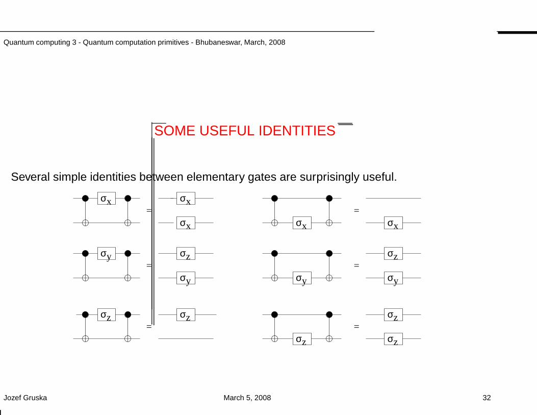
Quantum computing 3 - Quantum computation primitives - Bhubaneswar, March, 2008
SOME USEFUL IDENTITIES
Several simple identities between elementary gates are surprisingly useful.
sx =
s
s
x
x sx sx
=
s s
s s
s
s
y
y
z
y
z
y
= =
s s
s
s
s
z
z
z z
z
= =
Jozef Gruska March 5, 2008 32
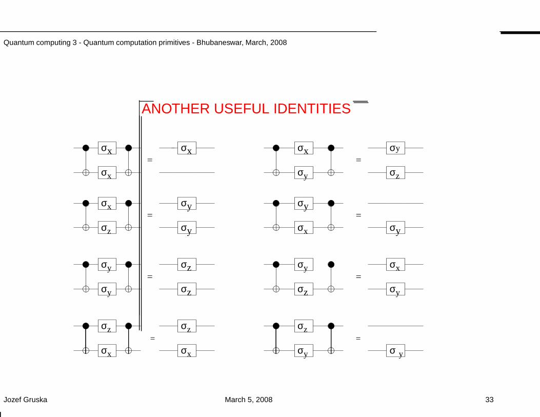
Quantum computing 3 - Quantum computation primitives - Bhubaneswar, March, 2008
ANOTHER USEFUL IDENTITIES
sx =
sx
s s=
s s
s s sy y
= =
s s
s
s
sz
= =
sx
sx
y
sy
z
s
x
z
y sy
x
s
y
y sz
z sy x
y
s
s
z
x
s
s
z
x
s
s s
z
y y
= =
Jozef Gruska March 5, 2008 33
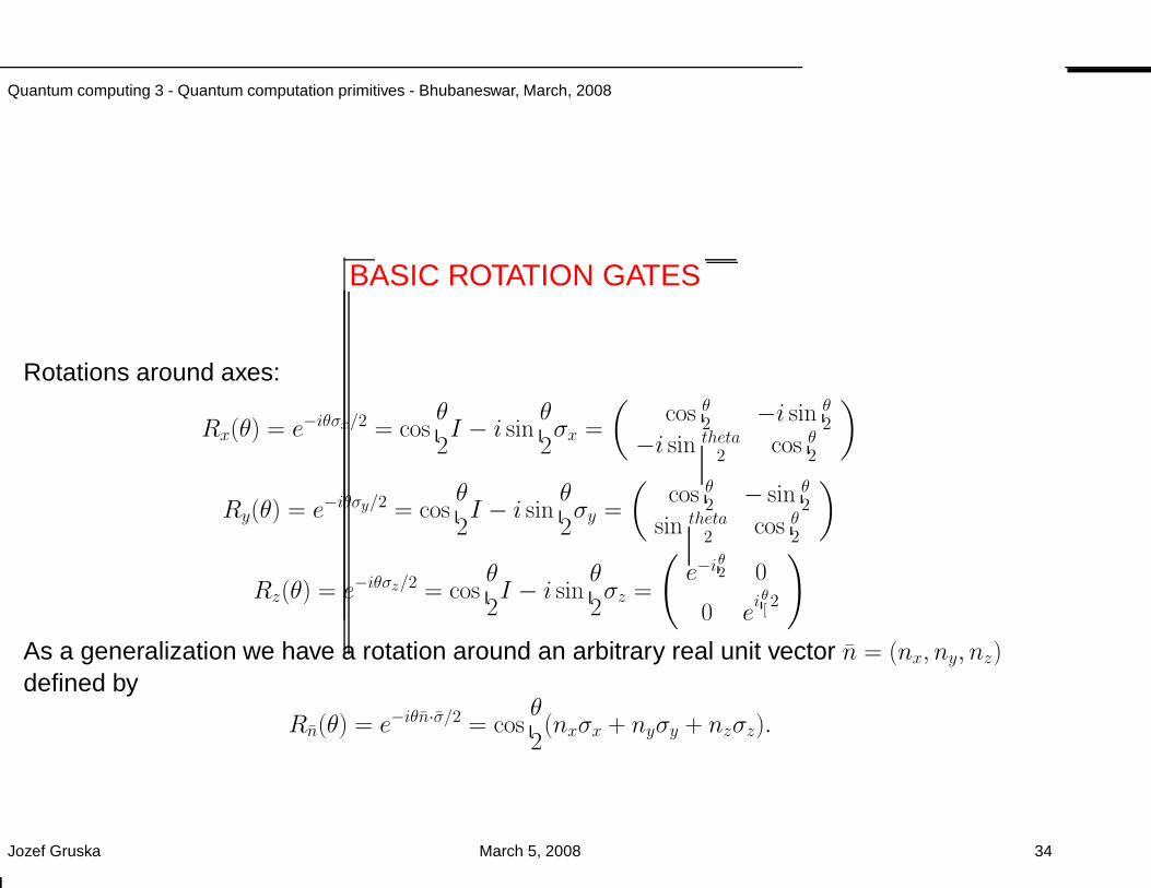
Quantum computing 3 - Quantum computation primitives - Bhubaneswar, March, 2008
BASIC ROTATION GATES
Rotations around axes:
Rx(θ) = e−iθσx/2 = cosθ
2I − i sin
θ
2σx =
(
cos θ2 −i sin θ2
−i sin theta2
cos θ2
)
Ry(θ) = e−iθσy/2 = cosθ
2I − i sin
θ
2σy =
(
cos θ2 − sin θ2
sin theta2
cos θ2
)
Rz(θ) = e−iθσz/2 = cosθ
2I − i sin
θ
2σz =
(
e−iθ2 0
0 eiθ[2
)
As a generalization we have a rotation around an arbitrary real unit vector n = (nx, ny, nz)
defined by
Rn(θ) = e−iθn·σ/2 = cosθ
2(nxσx + nyσy + nzσz).
Jozef Gruska March 5, 2008 34
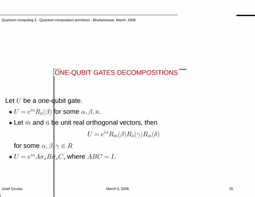
Quantum computing 3 - Quantum computation primitives - Bhubaneswar, March, 2008
ONE-QUBIT GATES DECOMPOSITIONS
Let U be a one-qubit gate.
• U = eiαRn(β) for some α, β, n.
• Let m and n be unit real orthogonal vectors, then
U = eiαRm(β)Rn(γ)Rm(δ)
for some α, β, γ ∈ R
• U = eiαAσxBσxC, where ABC = I.
Jozef Gruska March 5, 2008 35
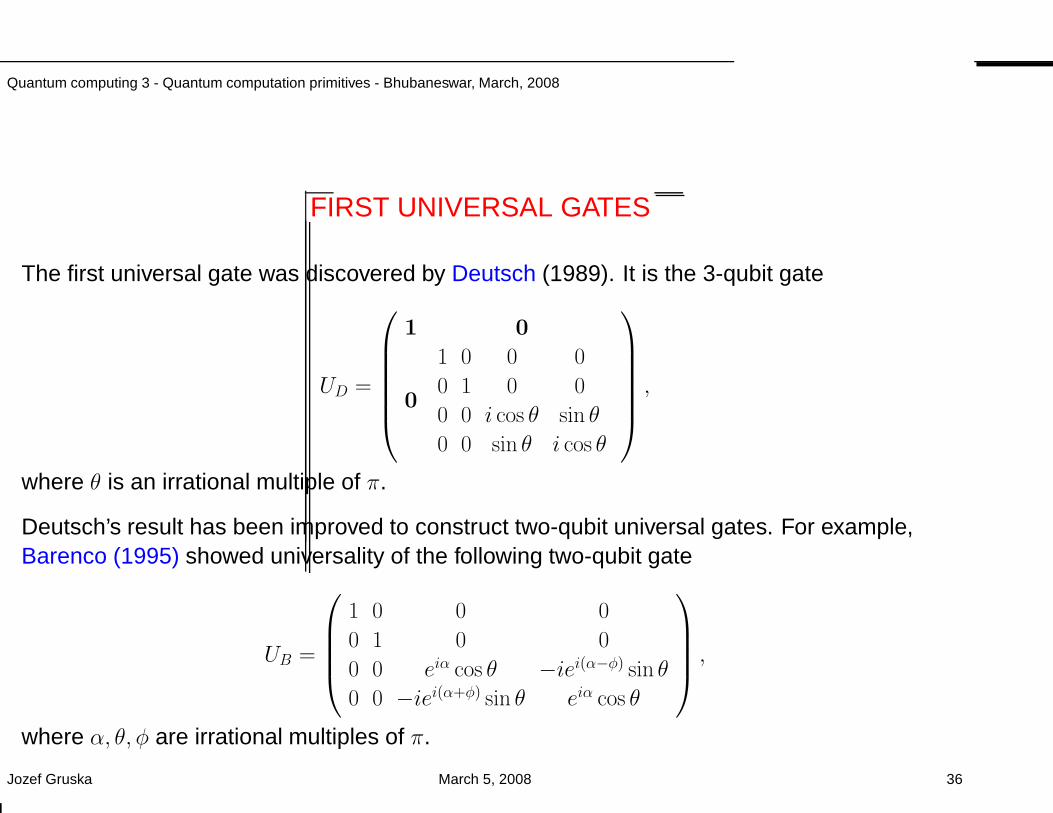
Quantum computing 3 - Quantum computation primitives - Bhubaneswar, March, 2008
FIRST UNIVERSAL GATES
The first universal gate was discovered by Deutsch (1989). It is the 3-qubit gate
UD =
1 0
0
1 0 0 0
0 1 0 0
0 0 i cos θ sin θ
0 0 sin θ i cos θ
,
where θ is an irrational multiple of π.
Deutsch’s result has been improved to construct two-qubit universal gates. For example,Barenco (1995) showed universality of the following two-qubit gate
UB =
1 0 0 0
0 1 0 0
0 0 eiα cos θ −iei(α−φ) sin θ
0 0 −iei(α+φ) sin θ eiα cos θ
,
where α, θ, φ are irrational multiples of π.
Jozef Gruska March 5, 2008 36
Quantum computing 3 - Quantum computation primitives - Bhubaneswar, March, 2008
Shortly afterwards, Barenco et al. (1995), Deutsch et al. (1995) and Lloyd (1995) showedthat all randomly chosen 2-qubit gate, but a set of measure zero, form, with their reverse,universal sets of gates.
Jozef Gruska March 5, 2008 37
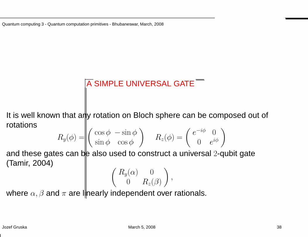
Quantum computing 3 - Quantum computation primitives - Bhubaneswar, March, 2008
A SIMPLE UNIVERSAL GATE
It is well known that any rotation on Bloch sphere can be composed out ofrotations
Ry(φ) =
(
cosφ − sinφsinφ cosφ
)
Rz(φ) =
(
e−iφ 00 eiφ
)
and these gates can be also used to construct a universal 2-qubit gate(Tamir, 2004)
(
Ry(α) 00 Rz(β)
)
,
where α, β and π are linearly independent over rationals.
Jozef Gruska March 5, 2008 38
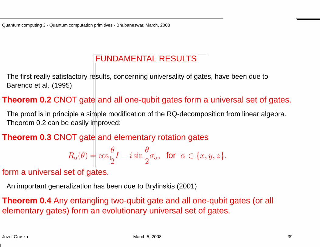
Quantum computing 3 - Quantum computation primitives - Bhubaneswar, March, 2008
FUNDAMENTAL RESULTS
The first really satisfactory results, concerning universality of gates, have been due toBarenco et al. (1995)
Theorem 0.2 CNOT gate and all one-qubit gates form a universal set of gates.
The proof is in principle a simple modification of the RQ-decomposition from linear algebra.Theorem 0.2 can be easily improved:
Theorem 0.3 CNOT gate and elementary rotation gates
Rα(θ) = cosθ
2I − i sin
θ
2σα, for α ∈ x, y, z.
form a universal set of gates.
An important generalization has been due to Brylinskis (2001)
Theorem 0.4 Any entangling two-qubit gate and all one-qubit gates (or allelementary gates) form an evolutionary universal set of gates.
Jozef Gruska March 5, 2008 39
Quantum computing 3 - Quantum computation primitives - Bhubaneswar, March, 2008
ENTANGLING GATES
• A two-qubit gate is called a entangling gate, or entangler, if it can map anunentangled state into an entangled one.
• Entangling is any two qubit gate that is not product of two one-qubit gatesand it is not locally equivalent to the SWAP gate.
• An entangling gate is called a perfect entangler if it can map a productstate into a maximally entangled state.
• CNOT and√
SWAP gates are perfect entanglers.
Jozef Gruska March 5, 2008 40
Quantum computing 3 - Quantum computation primitives - Bhubaneswar, March, 2008
COMMENTS
• CNOT gate is an important primitive in the optics-based quantuminformation processing.
• In case of superconductor- and spin-based quantum computing morebasic role play the gate
√SWAP. This gate is, similarly as the CNOT gate,
a maximally entangling gate.
• In general, for different technologies different two qubit gates or sets ofgates eiHt, for different t, generated by a Hamiltonian H, are considered aselementary and the circuit design task is then to decompose unitaries interms of these elementary gates and one-qubit gates.
Jozef Gruska March 5, 2008 41
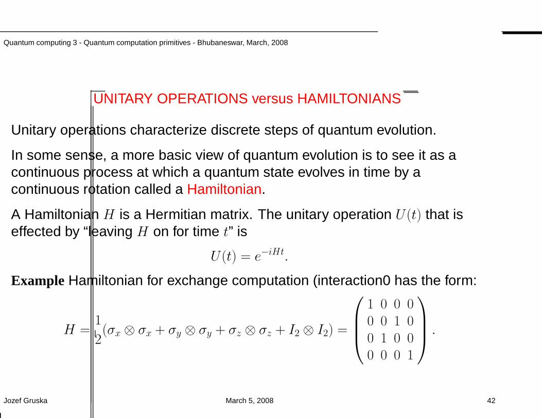
Quantum computing 3 - Quantum computation primitives - Bhubaneswar, March, 2008
UNITARY OPERATIONS versus HAMILTONIANS
Unitary operations characterize discrete steps of quantum evolution.
In some sense, a more basic view of quantum evolution is to see it as acontinuous process at which a quantum state evolves in time by acontinuous rotation called a Hamiltonian.
A Hamiltonian H is a Hermitian matrix. The unitary operation U (t) that iseffected by “leaving H on for time t” is
U (t) = e−iHt.
Example Hamiltonian for exchange computation (interaction0 has the form:
H =1
2(σx ⊗ σx + σy ⊗ σy + σz ⊗ σz + I2 ⊗ I2) =
1 0 0 00 0 1 00 1 0 00 0 0 1
.
Jozef Gruska March 5, 2008 42
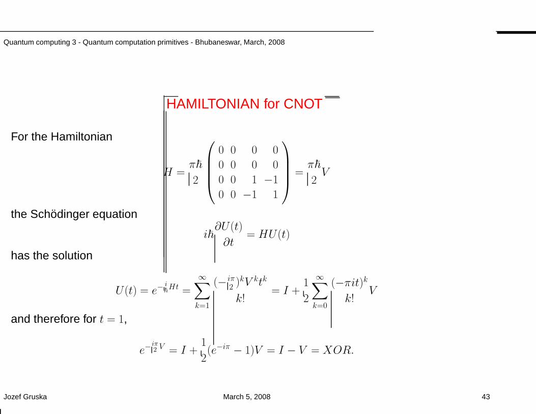
Quantum computing 3 - Quantum computation primitives - Bhubaneswar, March, 2008
HAMILTONIAN for CNOT
For the Hamiltonian
H =π~
2
0 0 0 0
0 0 0 0
0 0 1 −1
0 0 −1 1
=π~
2V
the Schodinger equation
i~∂U(t)
∂t= HU(t)
has the solution
U(t) = e−i~Ht =
∞∑
k=1
(− iπ2 )kV ktk
k!= I +
1
2
∞∑
k=0
(−πit)kk!
V
and therefore for t = 1,
e−iπ2 V = I +
1
2(e−iπ − 1)V = I − V = XOR.
Jozef Gruska March 5, 2008 43
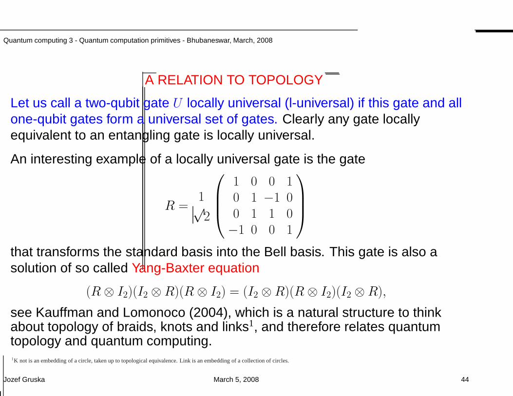
Quantum computing 3 - Quantum computation primitives - Bhubaneswar, March, 2008
A RELATION TO TOPOLOGY
Let us call a two-qubit gate U locally universal (l-universal) if this gate and allone-qubit gates form a universal set of gates. Clearly any gate locallyequivalent to an entangling gate is locally universal.
An interesting example of a locally universal gate is the gate
R =1√2
1 0 0 10 1 −1 00 1 1 0−1 0 0 1
that transforms the standard basis into the Bell basis. This gate is also asolution of so called Yang-Baxter equation
(R⊗ I2)(I2 ⊗R)(R ⊗ I2) = (I2 ⊗R)(R ⊗ I2)(I2 ⊗R),
see Kauffman and Lomonoco (2004), which is a natural structure to thinkabout topology of braids, knots and links1, and therefore relates quantumtopology and quantum computing.1K not is an embedding of a circle, taken up to topological equivalence. Link is an embedding of a collection of circles.
Jozef Gruska March 5, 2008 44
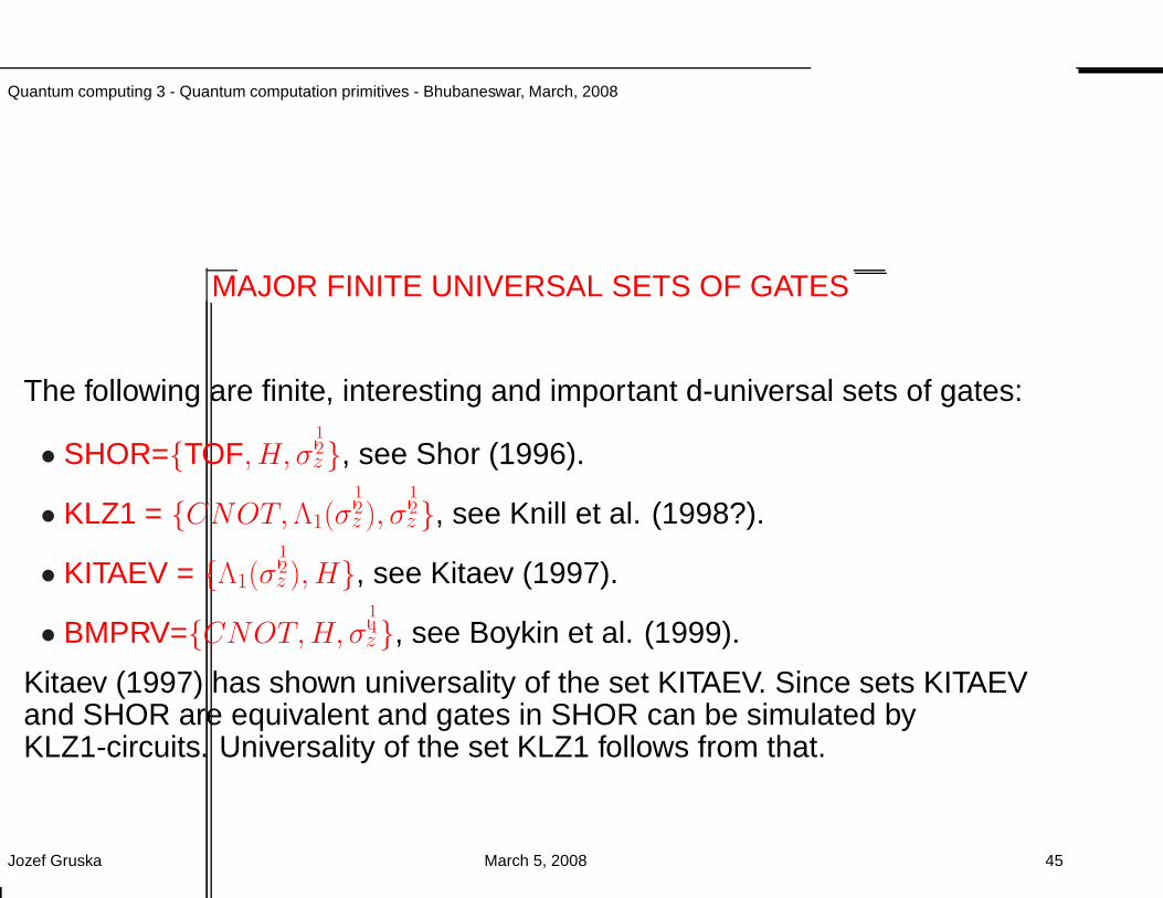
Quantum computing 3 - Quantum computation primitives - Bhubaneswar, March, 2008
MAJOR FINITE UNIVERSAL SETS OF GATES
The following are finite, interesting and important d-universal sets of gates:
• SHOR=TOF, H, σ12z, see Shor (1996).
• KLZ1 = CNOT,Λ1(σ12z ), σ
12z, see Knill et al. (1998?).
• KITAEV = Λ1(σ12z ), H, see Kitaev (1997).
• BMPRV=CNOT,H, σ14z, see Boykin et al. (1999).
Kitaev (1997) has shown universality of the set KITAEV. Since sets KITAEVand SHOR are equivalent and gates in SHOR can be simulated byKLZ1-circuits. Universality of the set KLZ1 follows from that.
Jozef Gruska March 5, 2008 45
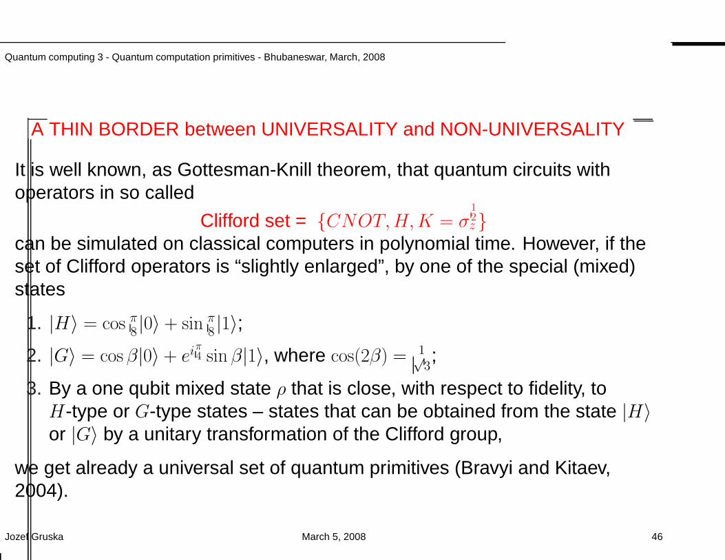
Quantum computing 3 - Quantum computation primitives - Bhubaneswar, March, 2008
A THIN BORDER between UNIVERSALITY and NON-UNIVERSALITY
It is well known, as Gottesman-Knill theorem, that quantum circuits withoperators in so called
Clifford set = CNOT,H,K = σ12z
can be simulated on classical computers in polynomial time. However, if theset of Clifford operators is “slightly enlarged”, by one of the special (mixed)states
1. |H〉 = cos π8|0〉 + sin π
8|1〉;
2. |G〉 = cos β|0〉 + eiπ4 sin β|1〉, where cos(2β) = 1√
3;
3. By a one qubit mixed state ρ that is close, with respect to fidelity, toH-type or G-type states – states that can be obtained from the state |H〉or |G〉 by a unitary transformation of the Clifford group,
we get already a universal set of quantum primitives (Bravyi and Kitaev,2004).
Jozef Gruska March 5, 2008 46
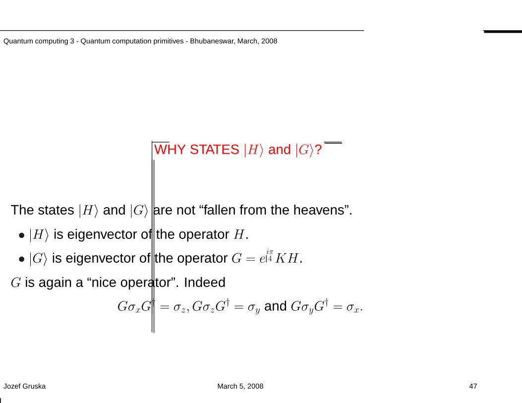
Quantum computing 3 - Quantum computation primitives - Bhubaneswar, March, 2008
WHY STATES |H〉 and |G〉?
The states |H〉 and |G〉 are not “fallen from the heavens”.
• |H〉 is eigenvector of the operator H.
• |G〉 is eigenvector of the operator G = eiπ4KH.
G is again a “nice operator”. Indeed
GσxG† = σz, GσzG
† = σy and GσyG† = σx.
Jozef Gruska March 5, 2008 47
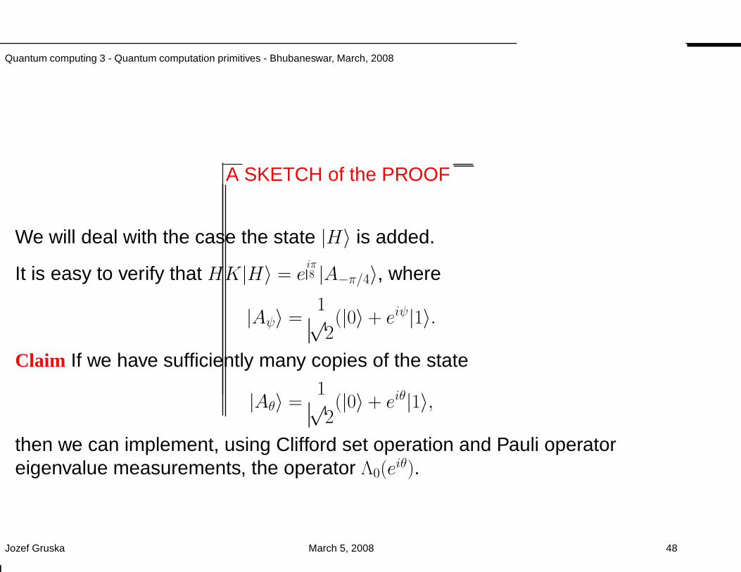
Quantum computing 3 - Quantum computation primitives - Bhubaneswar, March, 2008
A SKETCH of the PROOF
We will deal with the case the state |H〉 is added.
It is easy to verify that HK|H〉 = eiπ8 |A−π/4〉, where
|Aψ〉 =1√2(|0〉 + eiψ|1〉.
Claim If we have sufficiently many copies of the state
|Aθ〉 =1√2(|0〉 + eiθ|1〉,
then we can implement, using Clifford set operation and Pauli operatoreigenvalue measurements, the operator Λ0(e
iθ).
Jozef Gruska March 5, 2008 48
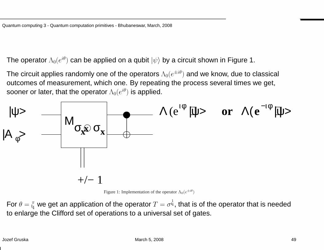
Quantum computing 3 - Quantum computation primitives - Bhubaneswar, March, 2008
The operator Λ0(eiθ) can be applied on a qubit |ψ〉 by a circuit shown in Figure 1.
The circuit applies randomly one of the operators Λ0(e±iθ) and we know, due to classical
outcomes of measurement, which one. By repeating the process several times we get,sooner or later, that the operator Λ0(e
iθ) is applied.
+/− 1
|ψ>
|A >φ
iφ )|ψ> or L( e−iφ )|ψ>Ms sx xx
(eL
Figure 1: Implementation of the operatorΛ0(e±iθ)
For θ = π4
we get an application of the operator T = σ14 , that is of the operator that is needed
to enlarge the Clifford set of operations to a universal set of gates.
Jozef Gruska March 5, 2008 49
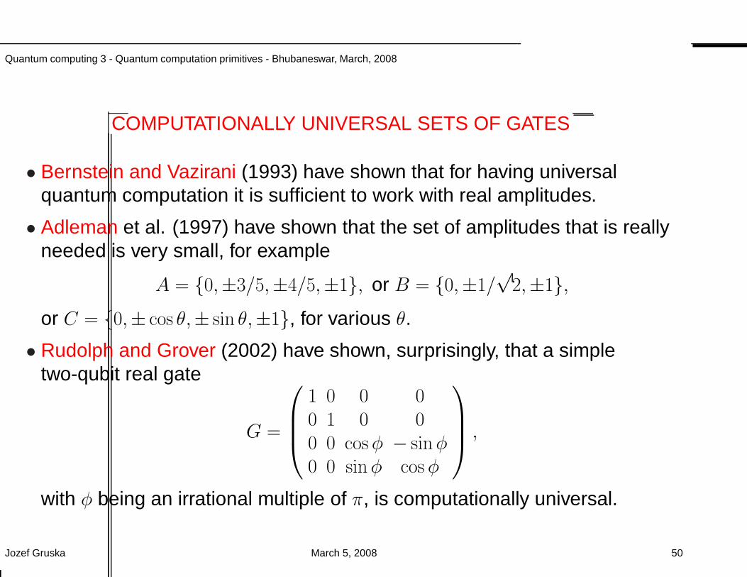
Quantum computing 3 - Quantum computation primitives - Bhubaneswar, March, 2008
COMPUTATIONALLY UNIVERSAL SETS OF GATES
• Bernstein and Vazirani (1993) have shown that for having universalquantum computation it is sufficient to work with real amplitudes.
• Adleman et al. (1997) have shown that the set of amplitudes that is reallyneeded is very small, for example
A = 0,±3/5,±4/5,±1, or B = 0,±1/√
2,±1,or C = 0,± cos θ,± sin θ,±1, for various θ.
• Rudolph and Grover (2002) have shown, surprisingly, that a simpletwo-qubit real gate
G =
1 0 0 00 1 0 00 0 cosφ − sinφ0 0 sinφ cosφ
,
with φ being an irrational multiple of π, is computationally universal.
Jozef Gruska March 5, 2008 50
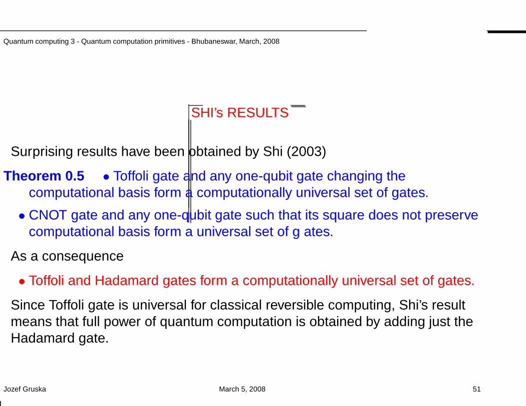
Quantum computing 3 - Quantum computation primitives - Bhubaneswar, March, 2008
SHI’s RESULTS
Surprising results have been obtained by Shi (2003)
Theorem 0.5 • Toffoli gate and any one-qubit gate changing thecomputational basis form a computationally universal set of gates.
• CNOT gate and any one-qubit gate such that its square does not preservecomputational basis form a universal set of g ates.
As a consequence
• Toffoli and Hadamard gates form a computationally universal set of gates.
Since Toffoli gate is universal for classical reversible computing, Shi’s resultmeans that full power of quantum computation is obtained by adding just theHadamard gate.
Jozef Gruska March 5, 2008 51
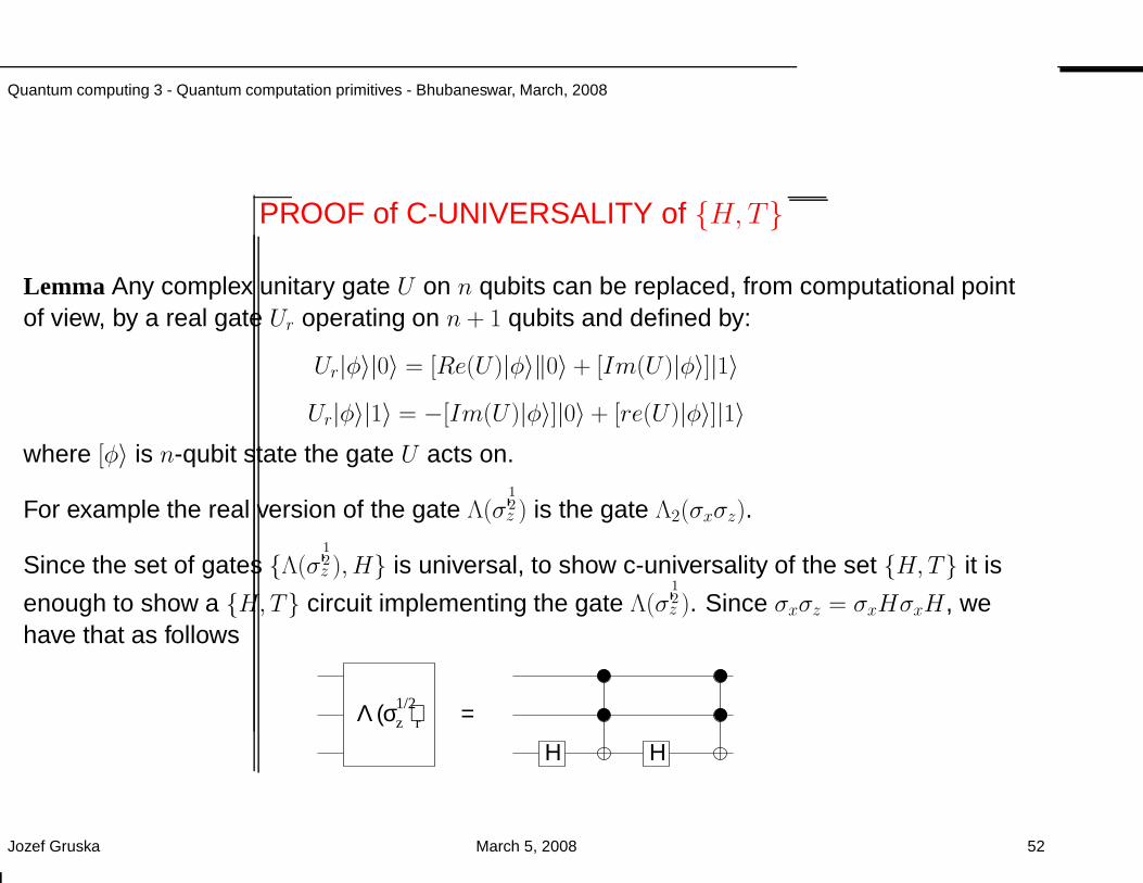
Quantum computing 3 - Quantum computation primitives - Bhubaneswar, March, 2008
PROOF of C-UNIVERSALITY of H,T
Lemma Any complex unitary gate U on n qubits can be replaced, from computational pointof view, by a real gate Ur operating on n + 1 qubits and defined by:
Ur|φ〉|0〉 = [Re(U)|φ〉‖0〉 + [Im(U)|φ〉]|1〉
Ur|φ〉|1〉 = −[Im(U)|φ〉]|0〉 + [re(U)|φ〉]|1〉where [φ〉 is n-qubit state the gate U acts on.
For example the real version of the gate Λ(σ12z ) is the gate Λ2(σxσz).
Since the set of gates Λ(σ12z ), H is universal, to show c-universality of the set H,T it is
enough to show a H,T circuit implementing the gate Λ(σ12z ). Since σxσz = σxHσxH, we
have that as follows
L (s z1/2)r =
Η Η
Jozef Gruska March 5, 2008 52
Quantum computing 3 - Quantum computation primitives - Bhubaneswar, March, 2008
POWER of the HADAMARD GATE
There are several ways to see what kind of power the Hadamard gaterepresents.
• On one side, Hadamard gate is a simple case of the Fourier transform andso one can say that, in some sense, quantum Fourier transform is whatdistinguishes classical and quantum computing.
• On the other hand, Hadamard gate can be seen as performing a randomcoin tossing and so one can say that it is just quantum random bit tossingwhat needs to be added to get quantum out of the classical computation.
Jozef Gruska March 5, 2008 53
Quantum computing 3 - Quantum computation primitives - Bhubaneswar, March, 2008
FAULT-TOLERANTLY UNIVERSAL SETS of GATES
• Informally, a fault-tolerantly universal set of gates is a universal set ofgates such that all gates of the set can operate in a noisy environment.
• More formal requirement is that there exists a quantum error correctingcode such that all gates of the set can be performed on logical qubitswithout a need to decode them first and in such a way that propagation ofsingle-qubit errors to other qubits in the same codeword is excluded.
The following sets of gates have been shown to be fault-tolerantly universal:
1. SHOR= T,H, σ12z, due to Shor (1996).
2. KITAEV =Λ1(σ12z ), H, due to Kitaev (1997).
3. BMPRV =CNOT,H, σ14z, due to Boykin et al. (1999).
Jozef Gruska March 5, 2008 54
Quantum computing 3 - Quantum computation primitives - Bhubaneswar, March, 2008
ENCODED UNIVERSALITY of EXCHANGE INTERACTIONS
• Encoded universality refers to the capability to generate, or toapproximate, all unitary matrices on a subspace of a Hilbert space createdby some logical qubits.
• Heisenberg physical nearest neighbor exchange interaction is notuniversal for quantum computation in general, but, surprisingly, it can beuniversal on properly encoded logical qubits.
Jozef Gruska March 5, 2008 55
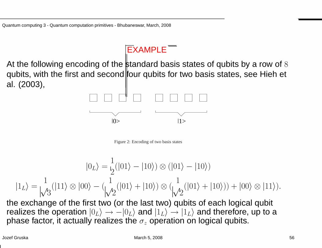
Quantum computing 3 - Quantum computation primitives - Bhubaneswar, March, 2008
EXAMPLE
At the following encoding of the standard basis states of qubits by a row of 8qubits, with the first and second four qubits for two basis states, see Hieh etal. (2003),
|1>|0>
Figure 2: Encoding of two basis states
|0L〉 =1
2(|01〉 − |10〉) ⊗ (|01〉 − |10〉)
|1L〉 =1√3(|11〉 ⊗ |00〉 − (
1√2(|01〉 + |10〉) ⊗ (
1√2(|01〉 + |10〉)) + |00〉 ⊗ |11〉).
the exchange of the first two (or the last two) qubits of each logical qubitrealizes the operation |0L〉 → −|0L〉 and |1L〉 → |1L〉 and therefore, up to aphase factor, it actually realizes the σz operation on logical qubits.
Jozef Gruska March 5, 2008 56
Quantum computing 3 - Quantum computation primitives - Bhubaneswar, March, 2008
One can then show that the Hamiltonian for σ1/4z operation, realized by the
nearing neighbors interactions is
eiπ8E1,2,
where
Ei,i+1 =1
2(σx,i ⊗ σx,i+1 + σy,i ⊗ σy,i+1 + σz,i ⊗ σz,i+1 + I ⊗ I)
is the interaction between ith and (i + 1)th qubit. With this notation an exactencoded Hadamard gate can be obtained as
H = eit1E1,2eit2E2,3eit1E1,2, where t1 =1
2arcsin
√
2
3and t2 = arccos
√
1
3.
To obtained an encoded realization of the CNOT gate, numerical methodshave been used (with 27 parallel nearest neighbor exchange interactions or50 serial gates).
As a consequence a single two qubit exchange interaction form a universalset (and therefore no one-qubit operations are needed) with respect to theencoded universality.
Jozef Gruska March 5, 2008 57
Quantum computing 3 - Quantum computation primitives - Bhubaneswar, March, 2008
UNIVERSAL HAMILTONIANS
• An n-qubit Hamiltonian is called (dynamically) universal, if it is able tosimulate any other n-qubit Hamiltonian using local unitaries.
• An n-qubit Hamiltonian is called entangling if every qubit is coupled to anyother qubit, directly or via intermediate qubits.
• Bremner et al. (2003) have shown that an entangling Hamiltonian isuniversal iff it contains at least one coupling term involving an evennumber of interacting qubits.
• They have shown that there are only two fundamentally different types ofentangling Hamiltonians on n qubits.
Jozef Gruska March 5, 2008 58
Quantum computing 3 - Quantum computation primitives - Bhubaneswar, March, 2008
PART II - OPTIMIZATION
Jozef Gruska March 5, 2008 59
Quantum computing 3 - Quantum computation primitives - Bhubaneswar, March, 2008
EFFICIENCY of UNIVERSAL SETS of QUANTUM PRIMITIVES
• It is a natural and important question to ask how good are, from the efficiency point ofview, different universal sets of quantum primitives.
• Lloyd (1995) have shown that number of base gates needed grows exponentially in lg 1/ε
to achieve precision ε.
• So called Solovay-Kitaev theorem implies that for evolutionary and computationaluniversality, it is not costly to replace one universal basis by another one – it requires onlypoly-logarithmic overhead in lg 1/ε and that that number of base gates are needed.
• Solovay-Kitaev result implies that any gate from one finite universal set can beapproximated with precision ε using polylog(1
ε) gates from other finite universal set of
gates. More exactly, Solovay and Kitaev showed that there exist polynomial timealgorithm (in lg 1/ε that creates a circuit with O(lgc(1/ε)) gates, where c ∈ [3, 4].)
• Harrow et al. (2002) have shown that for some sets of universal gates number of gatesrequired grows linearly in lg 1/ε (this is within a constant factor of the lower boundestablished by a counting argument).
• Of course, the above results are asymptotic and as such they have their limits.
Jozef Gruska March 5, 2008 60
Quantum computing 3 - Quantum computation primitives - Bhubaneswar, March, 2008
DECOMPOSITION of UNITARIES into ONE- and TWO-QUBIT GATES
Two very basic questions concerning decomposition of n-qubit unitaries intoone-and two-qubit gates are the following ones
• What is the total number of one-and two-qubits gates needed todecompose an arbitrary n qubit unitary operation – for different n?
• What is the total number of CNOT gates (or of some other entangling twoqubit gates) needed to decompose an arbitrary n qubit unitary – fordifferent n?
Jozef Gruska March 5, 2008 61
Quantum computing 3 - Quantum computation primitives - Bhubaneswar, March, 2008
GENERAL RESULTS
• Barenco et al. (1995) have shown that any n qubit gate can be realized byO(n34n) CNOT and one-qubit gates.
• The above result has been improved, step by step, to O(n24n), O(n4n) and,finally, by Vartiainen et al. (2003) to O(4n) – asymptotically tight.
• Concerning the CNOT gates only:
– The best known upper bound is O(4n) due to Vartiainen et al. (2003).– The best lower bound, due to Shende et al. (2003), is ⌈(4n − 3n− 1)/4⌉.
Jozef Gruska March 5, 2008 62
Quantum computing 3 - Quantum computation primitives - Bhubaneswar, March, 2008
DECOMPOSITION STEPS
• The basic idea of decomposition is borrowed from the QR-decompositionin linear algebra using so called Given’s rotation matrices Gi,j,k that are socalled “two-level matrices” which operate non-trivially only on j-th and k-thbasis vector and nullify elements on the i-th column and k-th row.
• The overall decomposition of a unitary ma trix U into a unit matrix has thenthe form
1∏
i=2n−1
2n∏
j=i+1
Gi,j,j−1
U = I.
• Each two-level matrix can then be implemented using Cn−1V and Cn−1NOTmatrices, where V is a unitary 2 × 2 matrix and CkV denotes a matrix withk control bits that control performance of the matrix V .
• A Cn−1V matrix can be implemented with O(n2) one- and two-qubit gates.Moreover, O(n) Cn−1NOT gates are needed between each two Cn−1Vgates and this leads to the total O(n34n) gates.
Jozef Gruska March 5, 2008 63
Quantum computing 3 - Quantum computation primitives - Bhubaneswar, March, 2008
• An improvement to O(4n) has been achieved when Gray-code ordering ofthe basis states has been used.
• An optimization method for quantum circuits, which is based on theexistence of the above decomposition, and which concentrates on anoptimization of the Cn−1NOT-gates is due to Aho and Svore (2003).
Jozef Gruska March 5, 2008 64
Quantum computing 3 - Quantum computation primitives - Bhubaneswar, March, 2008
RECURSIVE DECOMPOSITION METHOD
An important general and recursive method of decomposition of any unitarymatrix into one- and two-qubit unitary matrices, based on the Cartandecomposition of the Lie group su(2n), is due to Khaneja and Glaser (2000).
This methods has been used to obtain results presented below.
Jozef Gruska March 5, 2008 65
Quantum computing 3 - Quantum computation primitives - Bhubaneswar, March, 2008
OPTIMAL REALIZATION of TWO-QUBIT GATES
Main problems with optimal realization of two-qubit circuits can be formulated as follows.
• Given a fixed entangling two-qubit gate G, what is the smallest number ofgates G and of one-qubit (elementary) gates of a G-circuit forimplementation of an arbitrary given two-qubit gate U?
• Given a fixed entangling gate G, what is the minimal number of gates Gneeded, together with one-qubit gates, to realize an arbitrary two-qubitgate U?
• Given a fixed entangling gate G, find, as small as possible (with respect tothe number of gates G and one-qubit (elementary) gates), a universalcircuit scheme for implementation of any two-qubit unitary?
• To solve the above problems for special classes of entangling gates, or forspecific entangling gates, as CNOT, or double CNOT (DCNOT), or√
SWAP.
Jozef Gruska March 5, 2008 66
Quantum computing 3 - Quantum computation primitives - Bhubaneswar, March, 2008
• If G is an entangling two-qubit gate and nG is the minimal number of gatesG needed to realize (with one-qubit gates) any two-qubit gate, then for any1 ≤ k ≤ nG it is of interest to determine necessary and sufficient conditionsfor a two-qubit gate to have implementation by a circuit with k gates G andsome one-qubit gates.
Jozef Gruska March 5, 2008 67
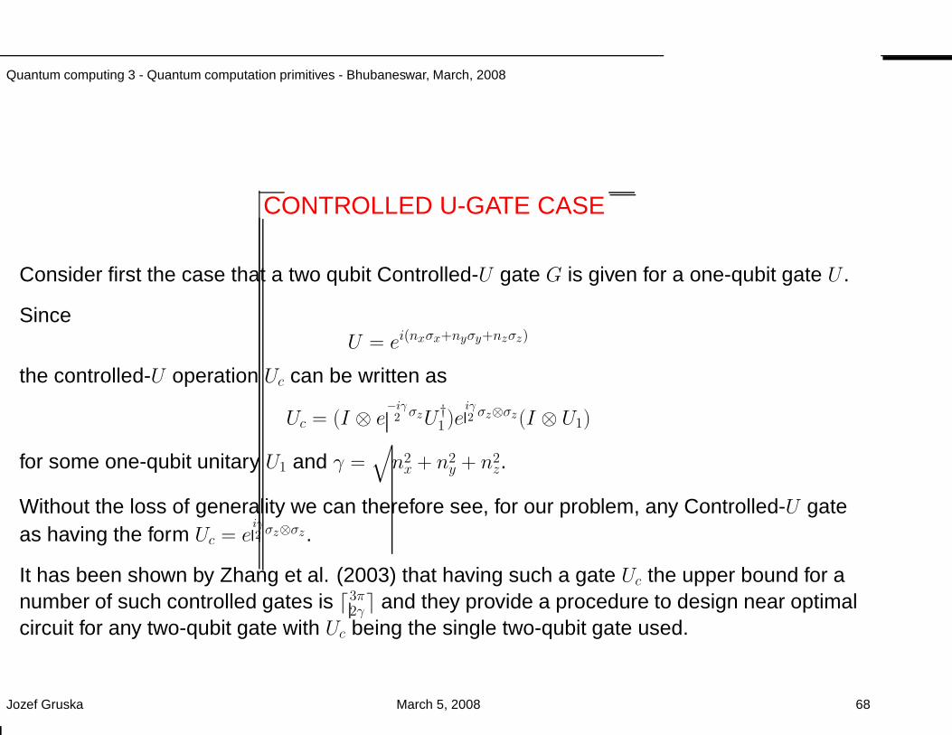
Quantum computing 3 - Quantum computation primitives - Bhubaneswar, March, 2008
CONTROLLED U-GATE CASE
Consider first the case that a two qubit Controlled-U gate G is given for a one-qubit gate U .
SinceU = ei(nxσx+nyσy+nzσz)
the controlled-U operation Uc can be written as
Uc = (I ⊗ e−iγ2 σzU †
1)eiγ2 σz⊗σz(I ⊗ U1)
for some one-qubit unitary U1 and γ =√
n2x + n2
y + n2z.
Without the loss of generality we can therefore see, for our problem, any Controlled-U gateas having the form Uc = e
iγ2 σz⊗σz .
It has been shown by Zhang et al. (2003) that having such a gate Uc the upper bound for anumber of such controlled gates is ⌈3π
2γ⌉ and they provide a procedure to design near optimalcircuit for any two-qubit gate with Uc being the single two-qubit gate used.
Jozef Gruska March 5, 2008 68
Quantum computing 3 - Quantum computation primitives - Bhubaneswar, March, 2008
KEY PROBLEMS
• The key problem is how many CNOT and one-qubit gates are necessaryand sufficient to implement any two-qubit gate.
• Since each one-qubit gate can be expressed as a composition of any twoof the elementary rotation gates Rx, Ry and Rz, it is of interest, and actuallyof large practical importance, to determine what is the minimal number of(elementary) gates Rx, Ry, Rz and CNOT needed to implement anarbitrary two-qubit gate.
Jozef Gruska March 5, 2008 69
Quantum computing 3 - Quantum computation primitives - Bhubaneswar, March, 2008
MAIN OUTCOMES
We discuss here only the best outcomes, so far, mainly due to Vidal and Dawson (2003),Shende et al. (2003 ) and Vatan and Williams (2003).
• 3 CNOT gates and 10 one-qubit and CNOT gates in total are sufficient torealize any two qubit gate.
• 3 CNOT gates and 9 gates in total are necessary.
• Each two-qubit gate can be realized using 3 CNOT gates and in total with18 gates from the set containing the CNOT gate and any two of the threegates from the set Rx, Ry, Rz. (The above result is optimal for the casetemporary storage is not allowed (because of being expensive).
• For gates from SO(4) only 12 gates Ry, Rz are needed.
Jozef Gruska March 5, 2008 70
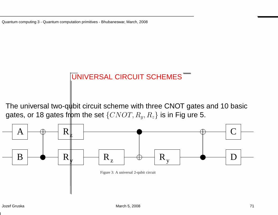
Quantum computing 3 - Quantum computation primitives - Bhubaneswar, March, 2008
UNIVERSAL CIRCUIT SCHEMES
The universal two-qubit circuit scheme with three CNOT gates and 10 basicgates, or 18 gates from the set CNOT,Ry, Rz is in Fig ure 5.
A
B
C
D R R
R z
R y z y
Figure 3: A universal2-qubit circuit
Jozef Gruska March 5, 2008 71
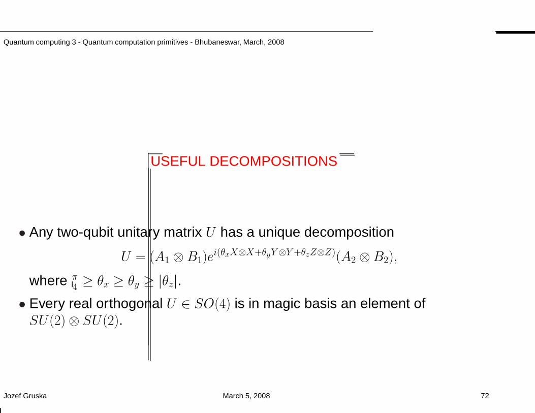
Quantum computing 3 - Quantum computation primitives - Bhubaneswar, March, 2008
USEFUL DECOMPOSITIONS
• Any two-qubit unitary matrix U has a unique decomposition
U = (A1 ⊗ B1)ei(θxX⊗X+θyY⊗Y+θzZ⊗Z)(A2 ⊗B2),
where π4 ≥ θx ≥ θy ≥ |θz|.
• Every real orthogonal U ∈ SO(4) is in magic basis an element ofSU (2) ⊗ SU (2).
Jozef Gruska March 5, 2008 72
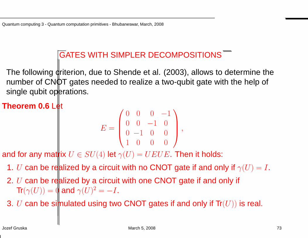
Quantum computing 3 - Quantum computation primitives - Bhubaneswar, March, 2008
GATES WITH SIMPLER DECOMPOSITIONS
The following criterion, due to Shende et al. (2003), allows to determine thenumber of CNOT gates needed to realize a two-qubit gate with the help ofsingle qubit operations.
Theorem 0.6 Let
E =
0 0 0 −10 0 −1 00 −1 0 01 0 0 0
,
and for any matrix U ∈ SU (4) let γ(U ) = UEUE. Then it holds:
1. U can be realized by a circuit with no CNOT gate if and only if γ(U ) = I.
2. U can be realized by a circuit with one CNOT gate if and only ifTr(γ(U )) = 0 and γ(U )2 = −I.
3. U can be simulated using two CNOT gates if and only if Tr(U )) is real.
Jozef Gruska March 5, 2008 73
Quantum computing 3 - Quantum computation primitives - Bhubaneswar, March, 2008
OPEN PROBLEMS
• Are there two two-qubit gates G1 and G2 such that any two-qubit gate canbe implemented by a circuit with one-qubit gates and at most two of thegates G1 and G2?
• Design an algorithm which constructs, for any two-qubit entangling gate U ,a minimal universal circuit scheme, with respect to the number of U gates,that uses U -gates as the only two qubit gates.
Jozef Gruska March 5, 2008 74
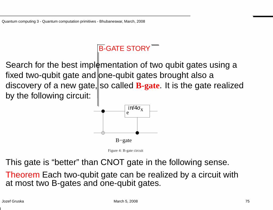
Quantum computing 3 - Quantum computation primitives - Bhubaneswar, March, 2008
B-GATE STORY
Search for the best implementation of two qubit gates using afixed two-qubit gate and one-qubit gates brought also adiscovery of a new gate, so called B-gate. It is the gate realizedby the following circuit:
eip/4sx
B−gate
Figure 4: B-gate circuit
This gate is “better” than CNOT gate in the following sense.
Theorem Each two-qubit gate can be realized by a circuit withat most two B-gates and one-qubit gates.
Jozef Gruska March 5, 2008 75
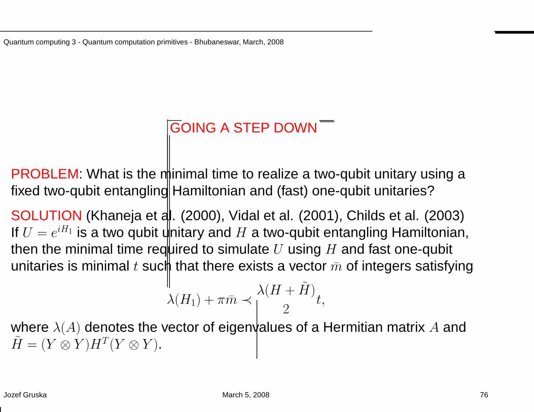
Quantum computing 3 - Quantum computation primitives - Bhubaneswar, March, 2008
GOING A STEP DOWN
PROBLEM: What is the minimal time to realize a two-qubit unitary using afixed two-qubit entangling Hamiltonian and (fast) one-qubit unitaries?
SOLUTION (Khaneja et al. (2000), Vidal et al. (2001), Childs et al. (2003)If U = eiH1 is a two qubit unitary and H a two-qubit entangling Hamiltonian,then the minimal time required to simulate U using H and fast one-qubitunitaries is minimal t such that there exists a vector m of integers satisfying
λ(H1) + πm ≺ λ(H + H)
2t,
where λ(A) denotes the vector of eigenvalues of a Hermitian matrix A andH = (Y ⊗ Y )HT (Y ⊗ Y ).
Jozef Gruska March 5, 2008 76
Quantum computing 3 - Quantum computation primitives - Bhubaneswar, March, 2008
3-QUBIT GATES CASE
• The case of an optimal realization of 3 qubits gates using a fixed two-qubitgate and one-qubit gates seems to be much more complex, but at thesame time much more important.
• A universal circuit scheme with 40 CNOT gates and 98 one-qubitelementary gates, Ry and Rz, due to Vatan and Williams (2004), is, so far,the most efficient general way of implementation of 3 qubit gates.
• The above mentioned universal 3-qubit circuit has been also obtainedusing the general, already mentioned. decomposition method of Khanejaand Glaser (2001) and therefore it is likely that a more efficient universalcircuit can be found.
Jozef Gruska March 5, 2008 77
Quantum computing 3 - Quantum computation primitives - Bhubaneswar, March, 2008
HOW MANY CNOT Are NEEDED TO GENERATE 3-QUBIT STATES?
• For two qubits one CNOT is enough to go from any pure state to any other.
• For three qubits three CNOT are enough to go from |000〉 to any other purestate.
• For three qubits two CNOT are enough to go from GHZ state to any otherpure state.
• As a corollary, four CNOT are enough to go from any 3-qubit state to any3-qubit state.
• Open problem: can the previous result be improved?
Jozef Gruska March 5, 2008 78
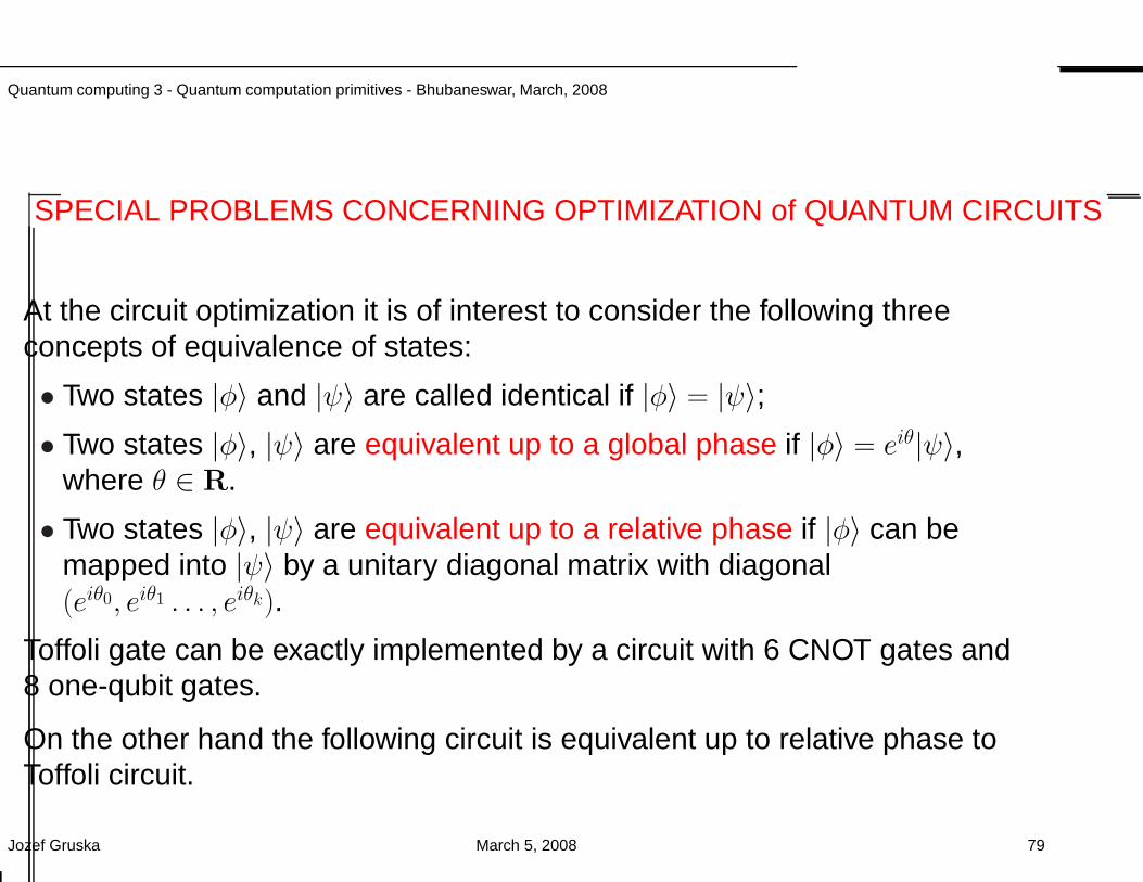
Quantum computing 3 - Quantum computation primitives - Bhubaneswar, March, 2008
SPECIAL PROBLEMS CONCERNING OPTIMIZATION of QUANTUM CIRCUITS
At the circuit optimization it is of interest to consider the following threeconcepts of equivalence of states:
• Two states |φ〉 and |ψ〉 are called identical if |φ〉 = |ψ〉;• Two states |φ〉, |ψ〉 are equivalent up to a global phase if |φ〉 = eiθ|ψ〉,
where θ ∈ R.
• Two states |φ〉, |ψ〉 are equivalent up to a relative phase if |φ〉 can bemapped into |ψ〉 by a unitary diagonal matrix with diagonal(eiθ0, eiθ1 . . . , eiθk).
Toffoli gate can be exactly implemented by a circuit with 6 CNOT gates and8 one-qubit gates.
On the other hand the following circuit is equivalent up to relative phase toToffoli circuit.
Jozef Gruska March 5, 2008 79
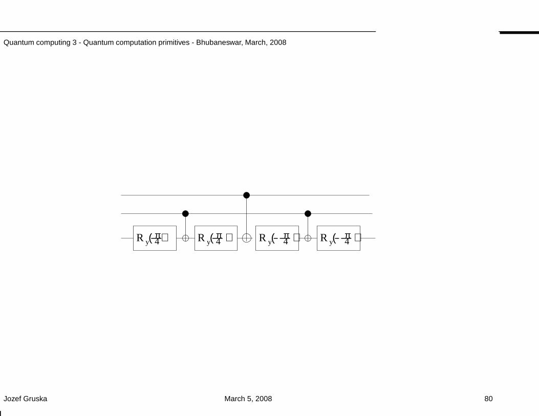
Quantum computing 3 - Quantum computation primitives - Bhubaneswar, March, 2008
R y( p4) R y( p
4 ) R y( p4 ) R y( p
4 )
Jozef Gruska March 5, 2008 80
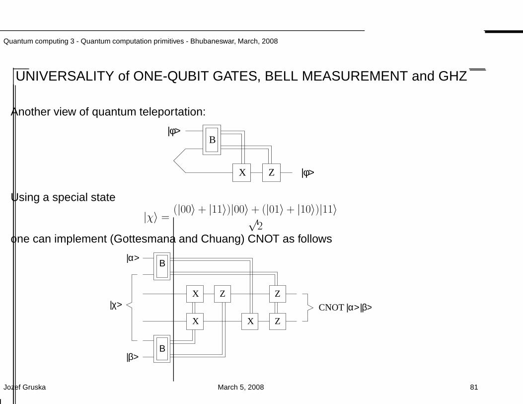
Quantum computing 3 - Quantum computation primitives - Bhubaneswar, March, 2008
UNIVERSALITY of ONE-QUBIT GATES, BELL MEASUREMENT and GHZ
Another view of quantum teleportation:
B
ZX
|φ>
|φ>
Using a special state
|χ〉 =(|00〉 + |11〉)|00〉 + (|01〉 + |10〉)|11〉√
2one can implement (Gottesmana and Chuang) CNOT as follows
B
B
|α>
|β>
CNOT |α>|β>Z
Z
X
X X
Z|c>
Jozef Gruska March 5, 2008 81
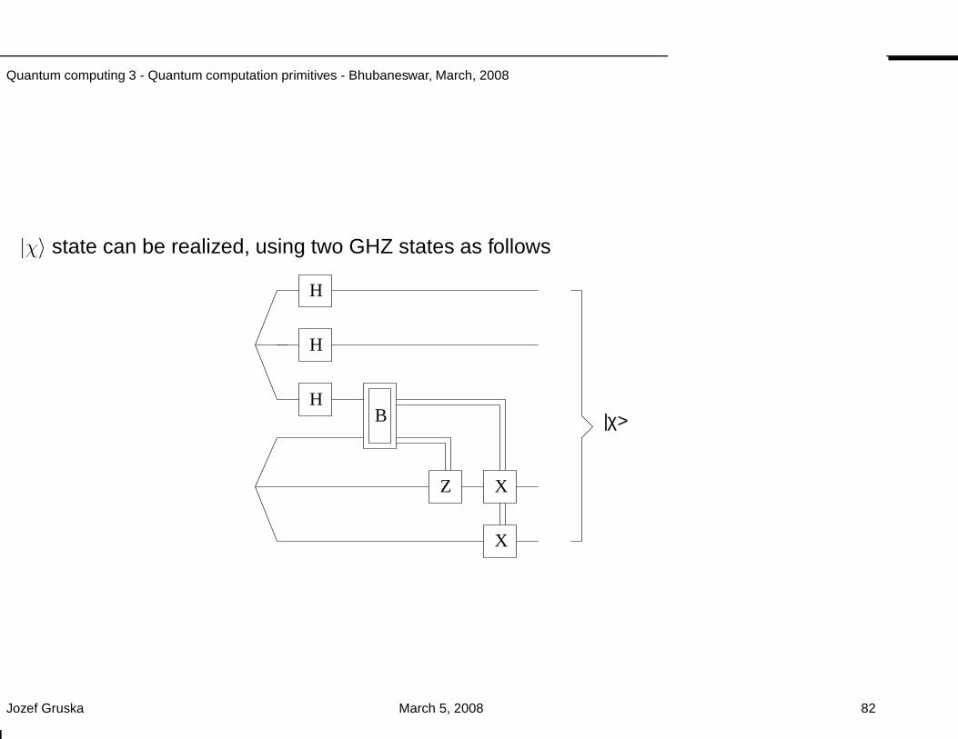
Quantum computing 3 - Quantum computation primitives - Bhubaneswar, March, 2008
|χ〉 state can be realized, using two GHZ states as follows
|c>
H
HB
X
Z X
H
Jozef Gruska March 5, 2008 82
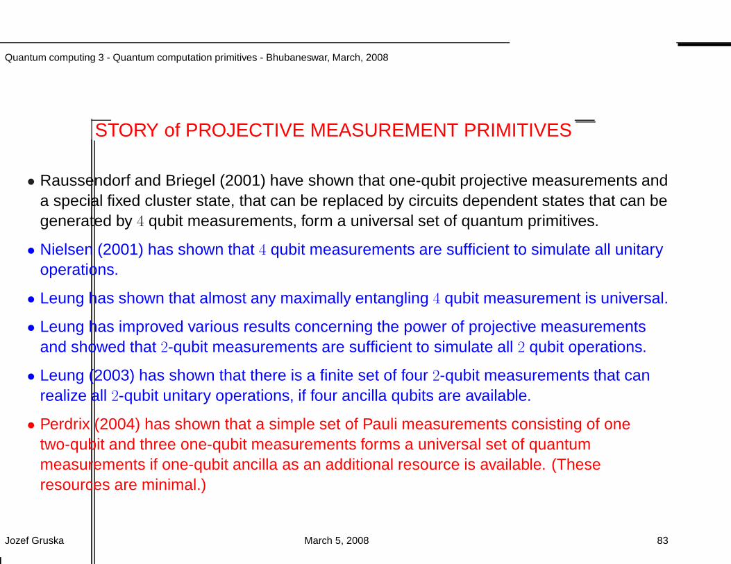
Quantum computing 3 - Quantum computation primitives - Bhubaneswar, March, 2008
STORY of PROJECTIVE MEASUREMENT PRIMITIVES
• Raussendorf and Briegel (2001) have shown that one-qubit projective measurements anda special fixed cluster state, that can be replaced by circuits dependent states that can begenerated by 4 qubit measurements, form a universal set of quantum primitives.
• Nielsen (2001) has shown that 4 qubit measurements are sufficient to simulate all unitaryoperations.
• Leung has shown that almost any maximally entangling 4 qubit measurement is universal.
• Leung has improved various results concerning the power of projective measurementsand showed that 2-qubit measurements are sufficient to simulate all 2 qubit operations.
• Leung (2003) has shown that there is a finite set of four 2-qubit measurements that canrealize all 2-qubit unitary operations, if four ancilla qubits are available.
• Perdrix (2004) has shown that a simple set of Pauli measurements consisting of onetwo-qubit and three one-qubit measurements forms a universal set of quantummeasurements if one-qubit ancilla as an additional resource is available. (Theseresources are minimal.)
Jozef Gruska March 5, 2008 83
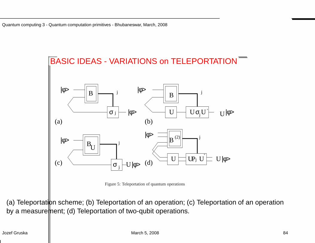
Quantum computing 3 - Quantum computation primitives - Bhubaneswar, March, 2008
BASIC IDEAS - VARIATIONS on TELEPORTATION
(a) (b)
(c) (d)
B
s
|φ> |φ>
|φ>
B
B
|φ>
|φ>
sU
U
U
sU UP
j |φ> U
j
j
U
j
j
j
B (2) j
j U +
U
+
U
|φ>
|φ>
Figure 5: Teleportation of quantum operations
(a) Teleportation scheme; (b) Teleportation of an operation; (c) Teleportation of an operationby a measurement; (d) Teleportation of two-qubit operations.
Jozef Gruska March 5, 2008 84
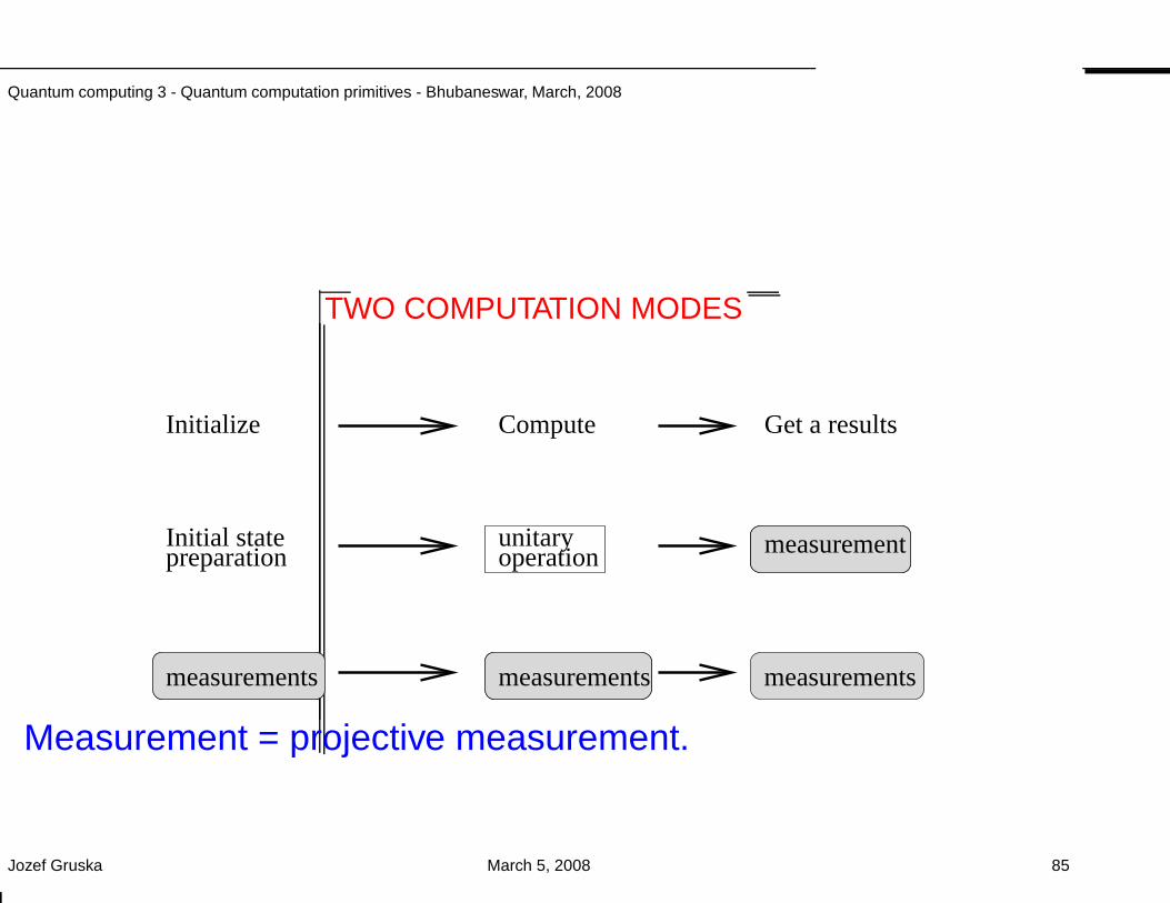
Quantum computing 3 - Quantum computation primitives - Bhubaneswar, March, 2008
TWO COMPUTATION MODES
Initial statepreparation
Initialize
measurements
Compute
operationunitary
Get a results
measurement
measurements measurements
Measurement = projective measurement.
Jozef Gruska March 5, 2008 85
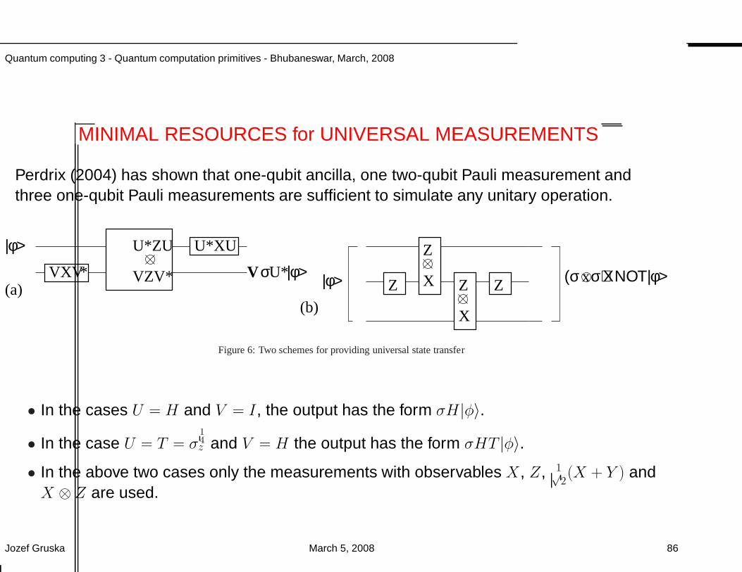
Quantum computing 3 - Quantum computation primitives - Bhubaneswar, March, 2008
MINIMAL RESOURCES for UNIVERSAL MEASUREMENTS
Perdrix (2004) has shown that one-qubit ancilla, one two-qubit Pauli measurement andthree one-qubit Pauli measurements are sufficient to simulate any unitary operation.
U*ZU
VZV* Z
Z
X
X
Z Z (s xs) CNOT|φ>
|φ>
*VXV
U*XU
V sU*|φ> |φ>(a)(b)
Figure 6: Two schemes for providing universal state transfer
• In the cases U = H and V = I, the output has the form σH|φ〉.
• In the case U = T = σ14z and V = H the output has the form σHT |φ〉.
• In the above two cases only the measurements with observables X, Z, 1√2(X + Y ) and
X ⊗ Z are used.
Jozef Gruska March 5, 2008 86
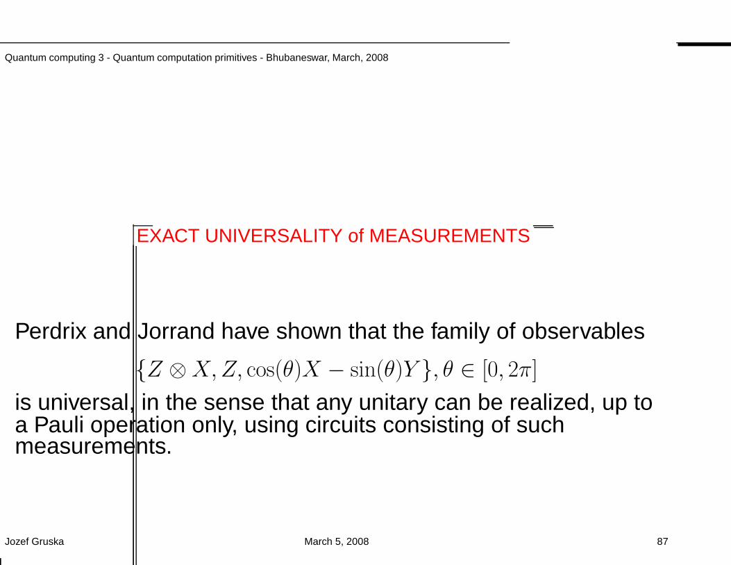
Quantum computing 3 - Quantum computation primitives - Bhubaneswar, March, 2008
EXACT UNIVERSALITY of MEASUREMENTS
Perdrix and Jorrand have shown that the family of observables
Z ⊗X,Z, cos(θ)X − sin(θ)Y , θ ∈ [0, 2π]
is universal, in the sense that any unitary can be realized, up toa Pauli operation only, using circuits consisting of suchmeasurements.
Jozef Gruska March 5, 2008 87
Quantum computing 3 - Quantum computation primitives - Bhubaneswar, March, 2008
OBSERVATIONS
• From strictly theoretical point of view closed quantum systems cannot becontrolled, because if one tries to control them, they necessarily becomeopen.
• Therefore, quantum measurement seem to be, in a sense, a unique tool toperform quantum computation.
Jozef Gruska March 5, 2008 88
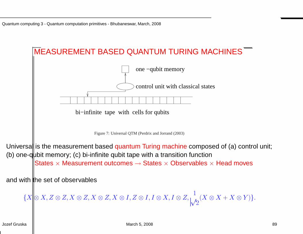
Quantum computing 3 - Quantum computation primitives - Bhubaneswar, March, 2008
MEASUREMENT BASED QUANTUM TURING MACHINES
one −qubit memory
control unit with classical states
tape with cells for qubitsbi−infinite
Figure 7: Universal QTM (Perdrix and Jorrand (2003)
Universal is the measurement based quantum Turing machine composed of (a) control unit;(b) one-qubit memory; (c) bi-infinite qubit tape with a transition function
States × Measurement outcomes → States × Observables × Head moves
and with the set of observables
X ⊗X,Z ⊗ Z,X ⊗ Z,X ⊗ Z,X ⊗ I, Z ⊗ I, I ⊗X, I ⊗ Z,1√2(X ⊗X +X ⊗ Y ).
Jozef Gruska March 5, 2008 89
Quantum computing 3 - Quantum computation primitives - Bhubaneswar, March, 2008
OPTICAL QUANTUM COMPUTATION PRIMITIVES
Knill, Laflamme and Milburn (2001) demonstrated that all-optical quantum computation inprinciple needs only
• beamsplitters;
• phase shifters;
• single photon sources;
• photodetectors with feedforward.
They suggested to realize entangling gate
• probabilistically using single photon detectors, linear optics and photodetectors;
• to improve probability of the gate performance using teleportation, to gate gate workingwith probability n2/(n + 1)2;
• to use farther error correction to improve probability of correct outcome.
Nielsen (2004) showed how to avoid last step using the idea of cluster states ofRaussendorf and Briegel.
Jozef Gruska March 5, 2008 90
Quantum computing 3 - Quantum computation primitives - Bhubaneswar, March, 2008
CLOSING OBSERVATION II
When a distinguished but elderly scientist states that somethingis possible, he is almost certainly right.
When he states that something is impossible,he is almost certainly wrong,
Arthur C. Clarke
Jozef Gruska March 5, 2008 91
Quantum computing 3 - Quantum computation primitives - Bhubaneswar, March, 2008
WISDOM
There is no quantum world. There is only an abstract quantumphysical description. It is wrong to think that the task of physicsis to find out how Nature is. Physics concerns what we can sayabout Nature.
Niels Bohr
Jozef Gruska March 5, 2008 92
Quantum computing 3 - Quantum computation primitives - Bhubaneswar, March, 2008
CLOSING MOTTO
Progress in science is often done by pessimists.Progress in technology is always done by optimists.
Jozef Gruska March 5, 2008 93
QUANTUM ALGORITHMS
Jozef Gruska
Faculty of Informatics
Brno
Czech Republic
March 6, 2008
Quantum computing 3, Quantum algorithms, Bhubaneshwar school, March 2008
3. QUANTUM ALGORITHMS
In the last two talks very basic techniques of designingquantum algorithms that are more efficient than theirclassical counterparts will be presented.
At first quantum algorithms for the Deutsch,Deutsch-Jozsa and Simon problems are presented andanalyzed.
Secondly, main Shor’s algorithms are analysed and theirgeneralisation is discussed.
Finally, Grover algorithm and generalisations andmodifications are presented and nalysed.
Jozef Gruska March 6, 2008 1
Quantum computing 3, Quantum algorithms, Bhubaneshwar school, March 2008
WHAT IS QUANTUM INFORMATION?
The views on what is quantum information differ.
• There is no quantum information, there are only quantum carriers ofclassical information. (A. Zeilinger).
• Concept of quantum information is primary fundamentalconcept/ingredient of quantum physics that cannot be defined.However, the viewpoint it suggest is richly suggestive, leading to newinteresting questions and interpretations of quantum processes. (J.Jozsa)
Jozef Gruska March 6, 2008 2
Quantum computing 3, Quantum algorithms, Bhubaneshwar school, March 2008
CLOSING OBSERVATION I
When a distinguished but elderly scientist states that something ispossible, he is almost certainly right.
When he states that something is impossible,he is almost certainly wrong,
Arthur C. Clarke
Jozef Gruska March 6, 2008 3
Quantum computing 3, Quantum algorithms, Bhubaneshwar school, March 2008
BASICS of QUANTUM ALGORITHMS and SIMPLE QUANTUM ALGORITHMS
Jozef Gruska March 6, 2008 4
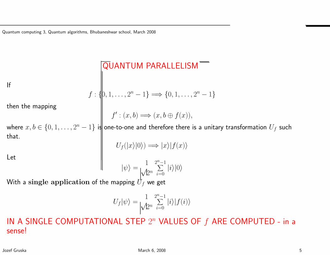
Quantum computing 3, Quantum algorithms, Bhubaneshwar school, March 2008
QUANTUM PARALLELISM
If
f : 0, 1, . . . , 2n − 1 =⇒ 0, 1, . . . , 2n − 1then the mapping
f ′ : (x, b) =⇒ (x, b⊕ f(x)),
where x, b ∈ 0, 1, . . . , 2n − 1 is one-to-one and therefore there is a unitary transformation Uf such
that.
Uf(|x〉|0〉) =⇒ |x〉|f(x)〉Let
|ψ〉 =1√2n
2n−1∑
i=0|i〉|0〉
With a single application of the mapping Uf we get
Uf |ψ〉 =1√2n
2n−1∑
i=0|i〉|f(i)〉
IN A SINGLE COMPUTATIONAL STEP 2n VALUES OF f ARE COMPUTED - in asense!
Jozef Gruska March 6, 2008 5
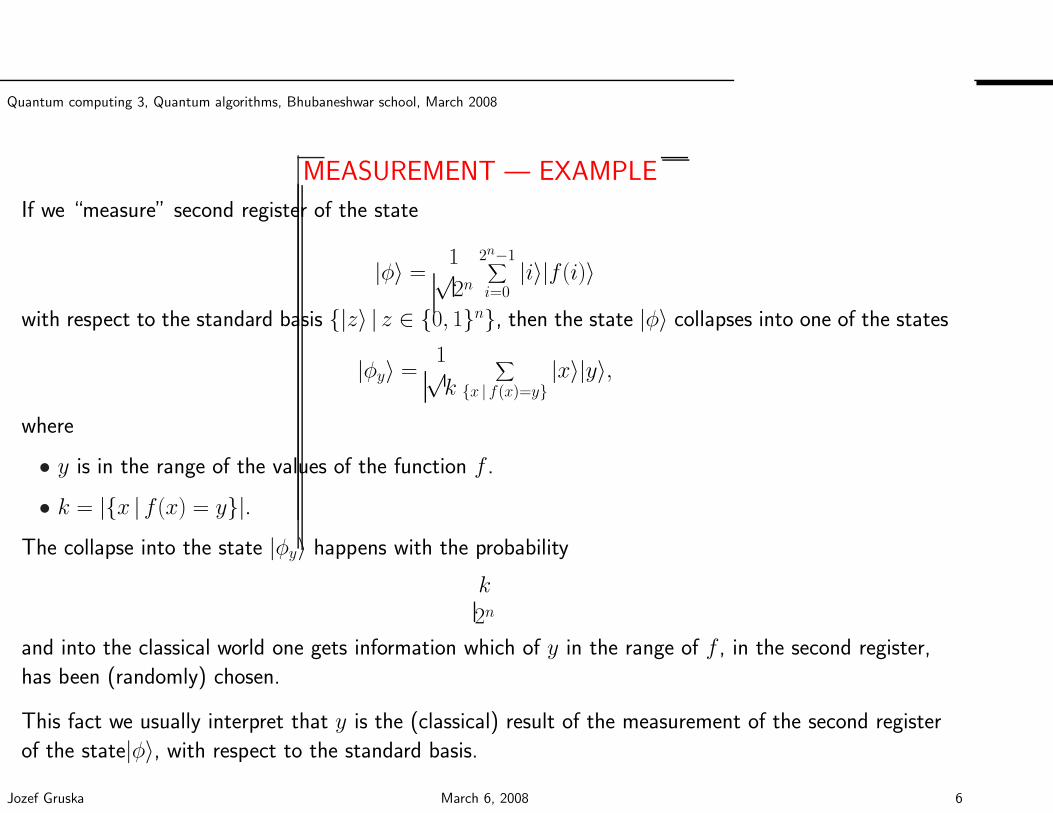
Quantum computing 3, Quantum algorithms, Bhubaneshwar school, March 2008
MEASUREMENT — EXAMPLE
If we “measure” second register of the state
|φ〉 =1√2n
2n−1∑
i=0|i〉|f(i)〉
with respect to the standard basis |z〉 | z ∈ 0, 1n, then the state |φ〉 collapses into one of the states
|φy〉 =1√k
∑
x | f(x)=y|x〉|y〉,
where
• y is in the range of the values of the function f .
• k = |x | f(x) = y|.The collapse into the state |φy〉 happens with the probability
k
2n
and into the classical world one gets information which of y in the range of f , in the second register,
has been (randomly) chosen.
This fact we usually interpret that y is the (classical) result of the measurement of the second register
of the state|φ〉, with respect to the standard basis.
Jozef Gruska March 6, 2008 6
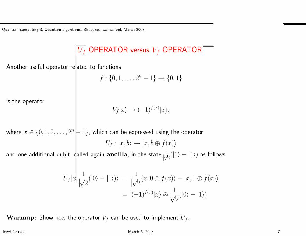
Quantum computing 3, Quantum algorithms, Bhubaneshwar school, March 2008
Uf OPERATOR versus Vf OPERATOR
Another useful operator related to functions
f : 0, 1, . . . , 2n − 1 → 0, 1
is the operator
Vf |x〉 → (−1)f(x)|x〉,
where x ∈ 0, 1, 2, . . . , 2n − 1, which can be expressed using the operator
Uf : |x, b〉 → |x, b⊕ f(x)〉and one additional qubit, called again ancilla, in the state 1√
2(|0〉 − |1〉) as follows
Uf |x,1√2(|0〉 − |1〉)〉 =
1√2(x, 0 ⊕ f(x)〉 − |x, 1 ⊕ f(x)〉
= (−1)f(x)|x〉 ⊗ 1√2(|0〉 − |1〉)
Warmup: Show how the operator Vf can be used to implement Uf .
Jozef Gruska March 6, 2008 7
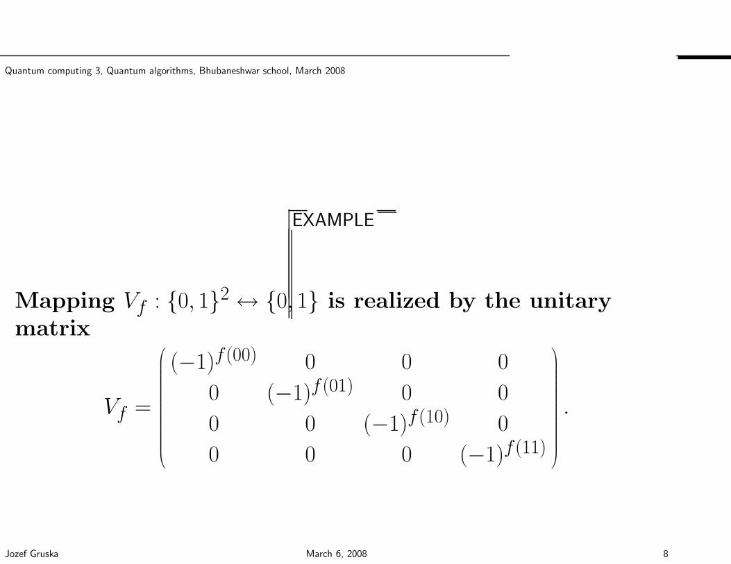
Quantum computing 3, Quantum algorithms, Bhubaneshwar school, March 2008
EXAMPLE
Mapping Vf : 0, 12 ↔ 0, 1 is realized by the unitarymatrix
Vf =
(−1)f(00) 0 0 0
0 (−1)f(01) 0 0
0 0 (−1)f(10) 0
0 0 0 (−1)f(11)
.
Jozef Gruska March 6, 2008 8
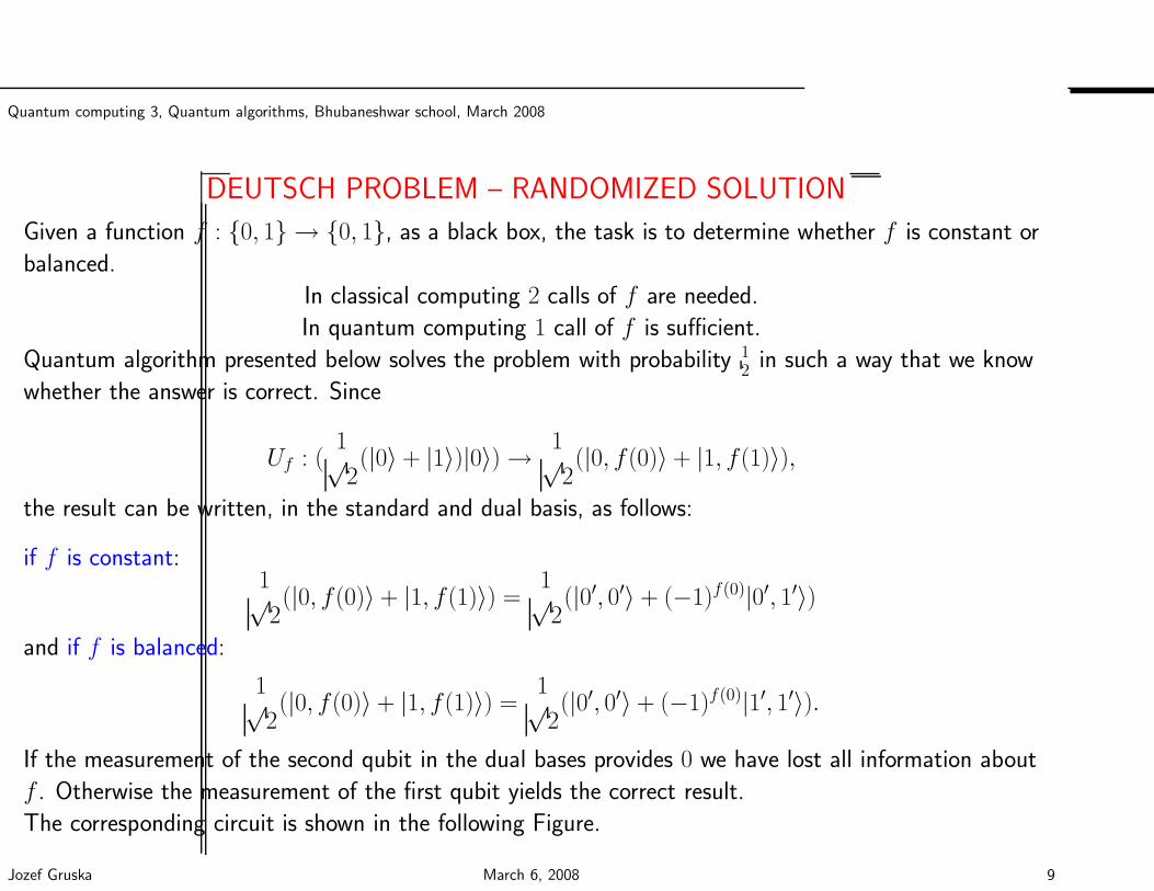
Quantum computing 3, Quantum algorithms, Bhubaneshwar school, March 2008
DEUTSCH PROBLEM – RANDOMIZED SOLUTION
Given a function f : 0, 1 → 0, 1, as a black box, the task is to determine whether f is constant or
balanced.
In classical computing 2 calls of f are needed.
In quantum computing 1 call of f is sufficient.
Quantum algorithm presented below solves the problem with probability 12 in such a way that we know
whether the answer is correct. Since
Uf : (1√2(|0〉 + |1〉)|0〉) → 1√
2(|0, f(0)〉 + |1, f(1)〉),
the result can be written, in the standard and dual basis, as follows:
if f is constant:1√2(|0, f(0)〉 + |1, f(1)〉) =
1√2(|0′, 0′〉 + (−1)f(0)|0′, 1′〉)
and if f is balanced:
1√2(|0, f(0)〉 + |1, f(1)〉) =
1√2(|0′, 0′〉 + (−1)f(0)|1′, 1′〉).
If the measurement of the second qubit in the dual bases provides 0 we have lost all information about
f . Otherwise the measurement of the first qubit yields the correct result.
The corresponding circuit is shown in the following Figure.
Jozef Gruska March 6, 2008 9
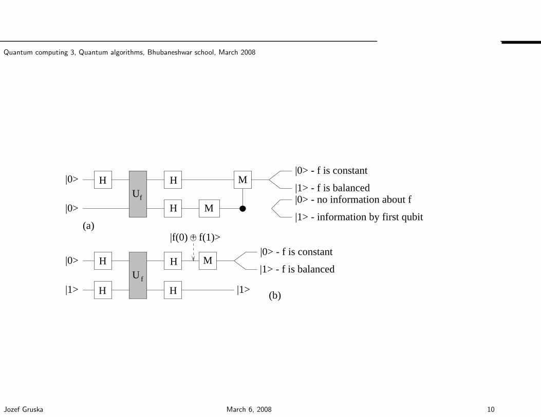
Quantum computing 3, Quantum algorithms, Bhubaneshwar school, March 2008
(a)
HU
U|1>
|0> - f is constant
|1> - f is balanced
(b)
f
f
|0> - f is constant
|1> - f is balanced|0> - no information about f
|f(0) + f(1)>
H H M
M
H H M
H H
|1> - information by first qubit
|0>
|0>
|0>
|1>
Jozef Gruska March 6, 2008 10
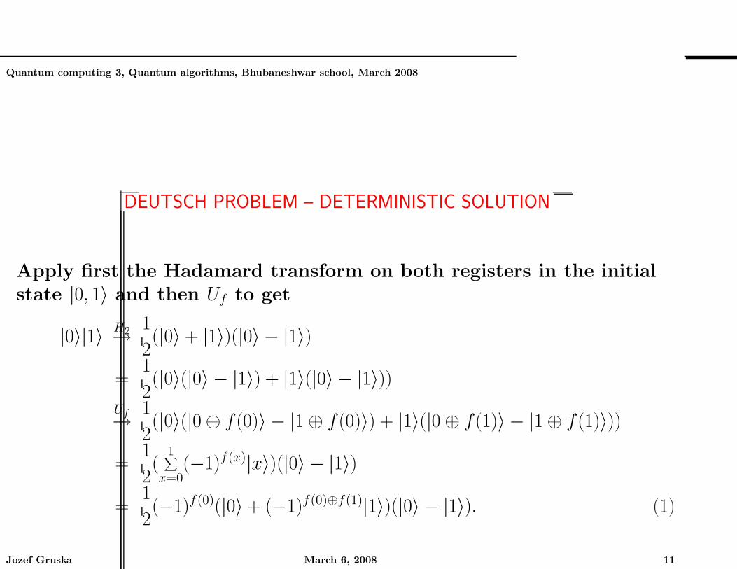
Quantum computing 3, Quantum algorithms, Bhubaneshwar school, March 2008
DEUTSCH PROBLEM – DETERMINISTIC SOLUTION
Apply first the Hadamard transform on both registers in the initialstate |0, 1〉 and then Uf to get
|0〉|1〉 H2→ 1
2(|0〉 + |1〉)(|0〉 − |1〉)
=1
2(|0〉(|0〉 − |1〉) + |1〉(|0〉 − |1〉))
Uf→ 1
2(|0〉(|0 ⊕ f(0)〉 − |1 ⊕ f(0)〉) + |1〉(|0 ⊕ f(1)〉 − |1 ⊕ f(1)〉))
=1
2(
1∑
x=0(−1)f(x)|x〉)(|0〉 − |1〉)
=1
2(−1)f(0)(|0〉 + (−1)f(0)⊕f(1)|1〉)(|0〉 − |1〉). (1)
Jozef Gruska March 6, 2008 11
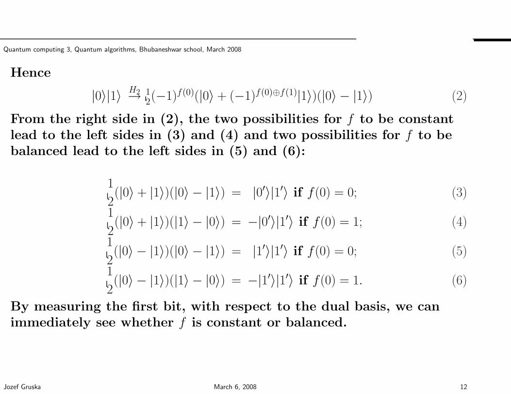
Quantum computing 3, Quantum algorithms, Bhubaneshwar school, March 2008
Hence
|0〉|1〉 H2→ 12(−1)f(0)(|0〉 + (−1)f(0)⊕f(1)|1〉)(|0〉 − |1〉) (2)
From the right side in (2), the two possibilities for f to be constantlead to the left sides in (3) and (4) and two possibilities for f to bebalanced lead to the left sides in (5) and (6):
1
2(|0〉 + |1〉)(|0〉 − |1〉) = |0′〉|1′〉 if f(0) = 0; (3)
1
2(|0〉 + |1〉)(|1〉 − |0〉) = −|0′〉|1′〉 if f(0) = 1; (4)
1
2(|0〉 − |1〉)(|0〉 − |1〉) = |1′〉|1′〉 if f(0) = 0; (5)
1
2(|0〉 − |1〉)(|1〉 − |0〉) = −|1′〉|1′〉 if f(0) = 1. (6)
By measuring the first bit, with respect to the dual basis, we canimmediately see whether f is constant or balanced.
Jozef Gruska March 6, 2008 12
Quantum computing 3, Quantum algorithms, Bhubaneshwar school, March 2008
SOMETIMES USEFUL WISDOM
If you are able to show that something
is imposssible
then, as the next step, it is often useful to try to show that
it is actually possible
from some other, useful, or at least interesting, point of view.
Jozef Gruska March 6, 2008 13
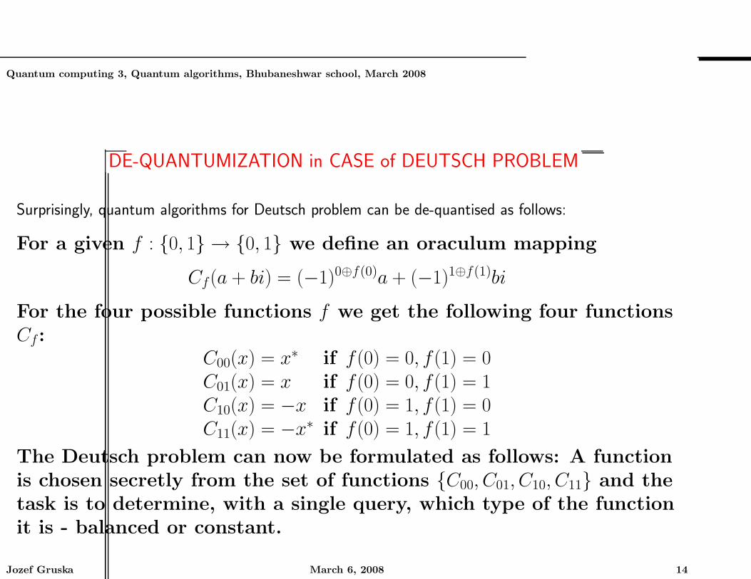
Quantum computing 3, Quantum algorithms, Bhubaneshwar school, March 2008
DE-QUANTUMIZATION in CASE of DEUTSCH PROBLEM
Surprisingly, quantum algorithms for Deutsch problem can be de-quantised as follows:
For a given f : 0, 1 → 0, 1 we define an oraculum mapping
Cf(a + bi) = (−1)0⊕f(0)a + (−1)1⊕f(1)bi
For the four possible functions f we get the following four functionsCf :
C00(x) = x∗ if f(0) = 0, f(1) = 0C01(x) = x if f(0) = 0, f(1) = 1C10(x) = −x if f(0) = 1, f(1) = 0C11(x) = −x∗ if f(0) = 1, f(1) = 1
The Deutsch problem can now be formulated as follows: A functionis chosen secretly from the set of functions C00, C01, C10, C11 and thetask is to determine, with a single query, which type of the functionit is - balanced or constant.
Jozef Gruska March 6, 2008 14
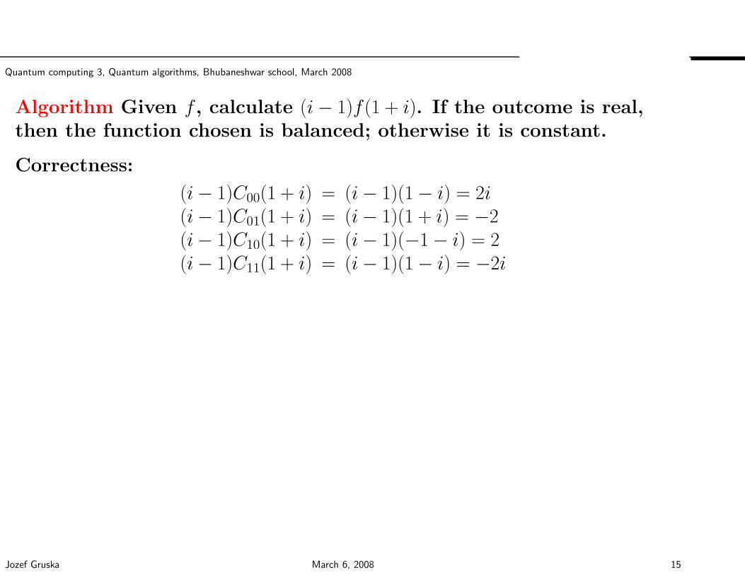
Quantum computing 3, Quantum algorithms, Bhubaneshwar school, March 2008
Algorithm Given f , calculate (i− 1)f(1 + i). If the outcome is real,then the function chosen is balanced; otherwise it is constant.
Correctness:
(i− 1)C00(1 + i) = (i− 1)(1 − i) = 2i(i− 1)C01(1 + i) = (i− 1)(1 + i) = −2(i− 1)C10(1 + i) = (i− 1)(−1 − i) = 2(i− 1)C11(1 + i) = (i− 1)(1 − i) = −2i
Jozef Gruska March 6, 2008 15
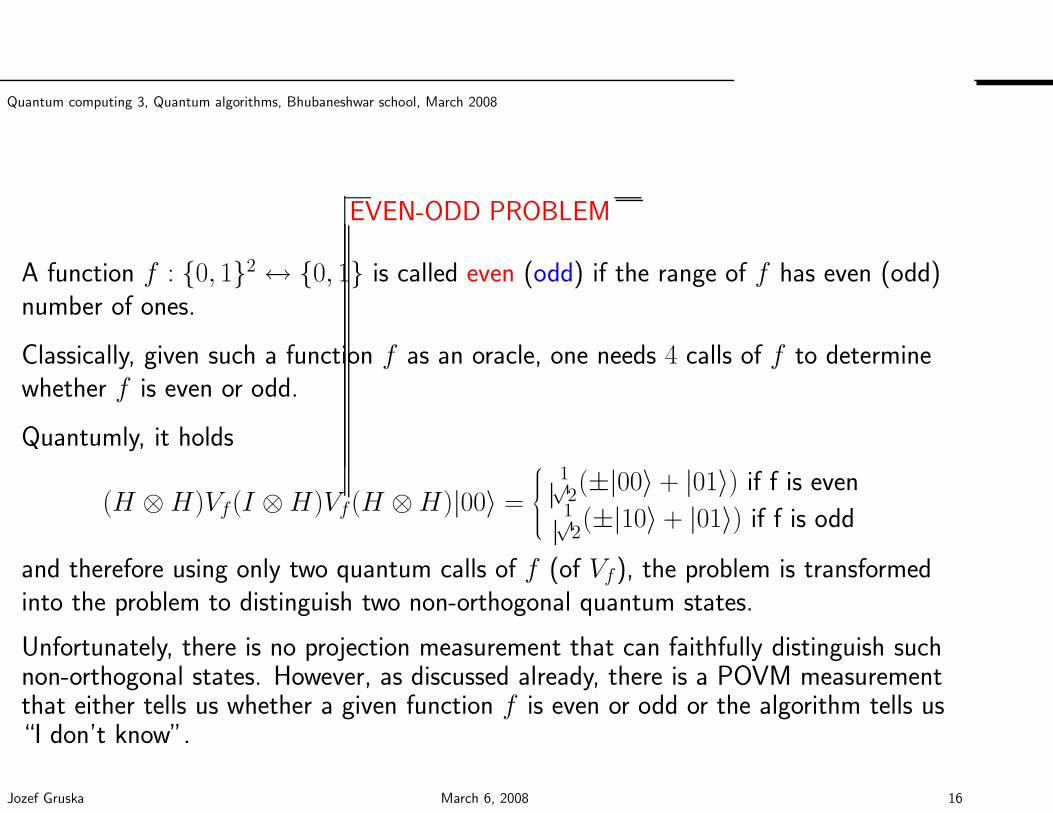
Quantum computing 3, Quantum algorithms, Bhubaneshwar school, March 2008
EVEN-ODD PROBLEM
A function f : 0, 12 ↔ 0, 1 is called even (odd) if the range of f has even (odd)number of ones.
Classically, given such a function f as an oracle, one needs 4 calls of f to determinewhether f is even or odd.
Quantumly, it holds
(H ⊗H)Vf(I ⊗H)Vf(H ⊗H)|00〉 =
1√2(±|00〉 + |01〉) if f is even
1√2(±|10〉 + |01〉) if f is odd
and therefore using only two quantum calls of f (of Vf), the problem is transformedinto the problem to distinguish two non-orthogonal quantum states.
Unfortunately, there is no projection measurement that can faithfully distinguish suchnon-orthogonal states. However, as discussed already, there is a POVM measurementthat either tells us whether a given function f is even or odd or the algorithm tells us“I don’t know”.
Jozef Gruska March 6, 2008 16
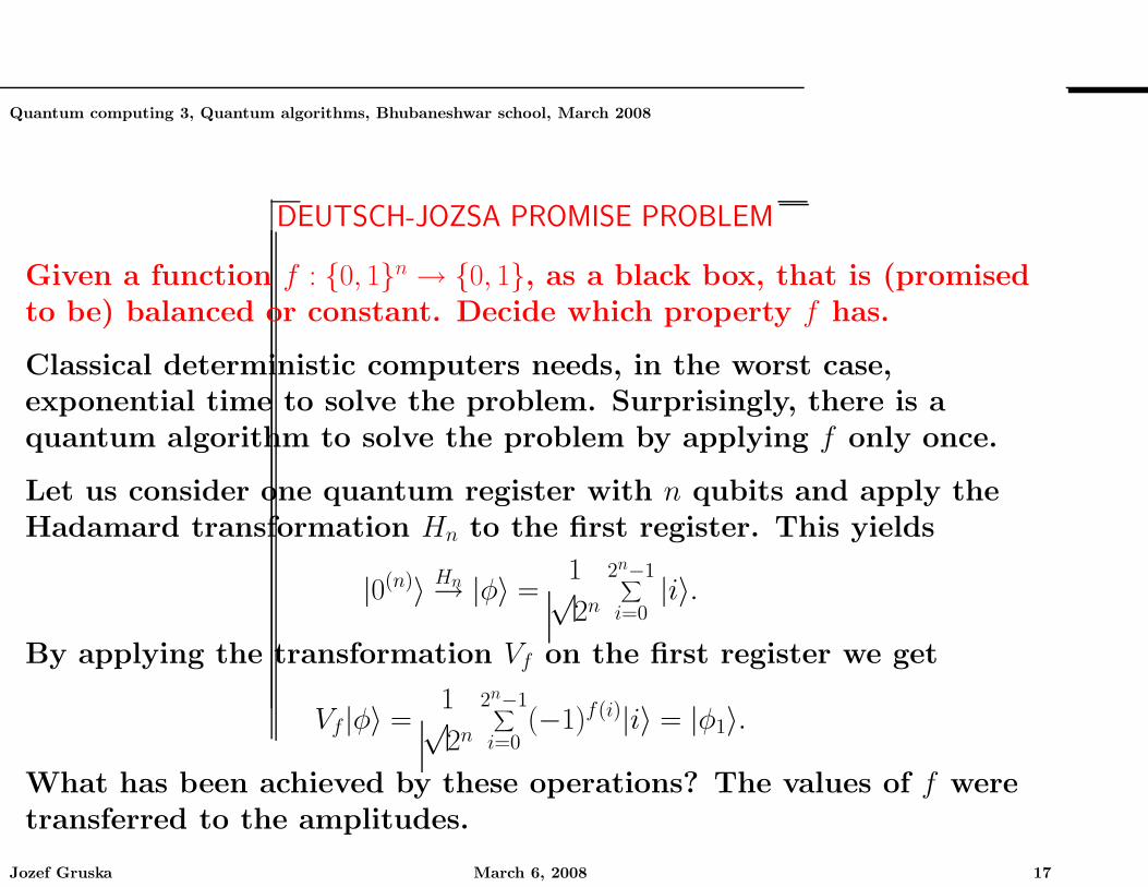
Quantum computing 3, Quantum algorithms, Bhubaneshwar school, March 2008
DEUTSCH-JOZSA PROMISE PROBLEM
Given a function f : 0, 1n → 0, 1, as a black box, that is (promisedto be) balanced or constant. Decide which property f has.
Classical deterministic computers needs, in the worst case,exponential time to solve the problem. Surprisingly, there is aquantum algorithm to solve the problem by applying f only once.
Let us consider one quantum register with n qubits and apply theHadamard transformation Hn to the first register. This yields
|0(n)〉 Hn→ |φ〉 =1√2n
2n−1∑
i=0|i〉.
By applying the transformation Vf on the first register we get
Vf |φ〉 =1√2n
2n−1∑
i=0(−1)f(i)|i〉 = |φ1〉.
What has been achieved by these operations? The values of f weretransferred to the amplitudes.
Jozef Gruska March 6, 2008 17
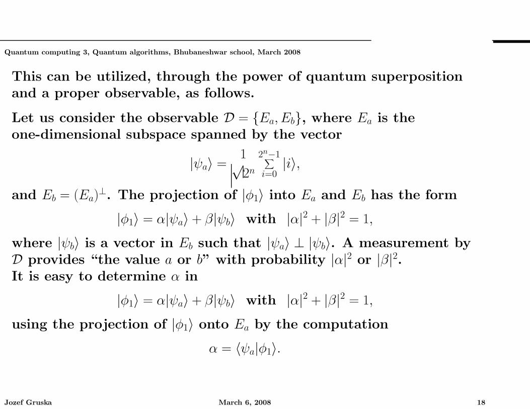
Quantum computing 3, Quantum algorithms, Bhubaneshwar school, March 2008
This can be utilized, through the power of quantum superpositionand a proper observable, as follows.
Let us consider the observable D = Ea, Eb, where Ea is theone-dimensional subspace spanned by the vector
|ψa〉 =1√2n
2n−1∑
i=0|i〉,
and Eb = (Ea)⊥. The projection of |φ1〉 into Ea and Eb has the form
|φ1〉 = α|ψa〉 + β|ψb〉 with |α|2 + |β|2 = 1,
where |ψb〉 is a vector in Eb such that |ψa〉 ⊥ |ψb〉. A measurement byD provides “the value a or b” with probability |α|2 or |β|2.It is easy to determine α in
|φ1〉 = α|ψa〉 + β|ψb〉 with |α|2 + |β|2 = 1,
using the projection of |φ1〉 onto Ea by the computation
α = 〈ψa|φ1〉.
Jozef Gruska March 6, 2008 18
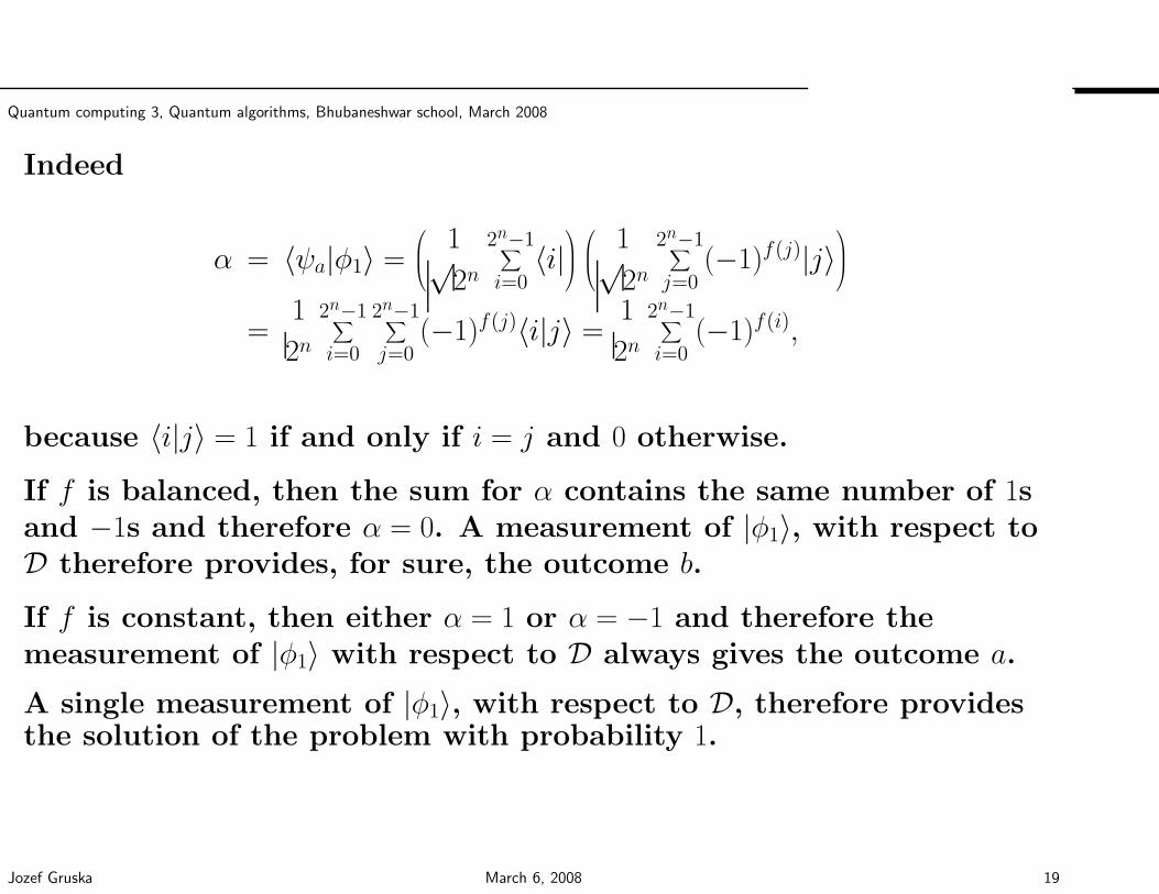
Quantum computing 3, Quantum algorithms, Bhubaneshwar school, March 2008
Indeed
α = 〈ψa|φ1〉 =
1√2n
2n−1∑
i=0〈i|
1√2n
2n−1∑
j=0(−1)f(j)|j〉
=1
2n2n−1
∑
i=0
2n−1∑
j=0(−1)f(j)〈i|j〉 =
1
2n2n−1
∑
i=0(−1)f(i),
because 〈i|j〉 = 1 if and only if i = j and 0 otherwise.
If f is balanced, then the sum for α contains the same number of 1sand −1s and therefore α = 0. A measurement of |φ1〉, with respect toD therefore provides, for sure, the outcome b.
If f is constant, then either α = 1 or α = −1 and therefore themeasurement of |φ1〉 with respect to D always gives the outcome a.
A single measurement of |φ1〉, with respect to D, therefore providesthe solution of the problem with probability 1.
Jozef Gruska March 6, 2008 19
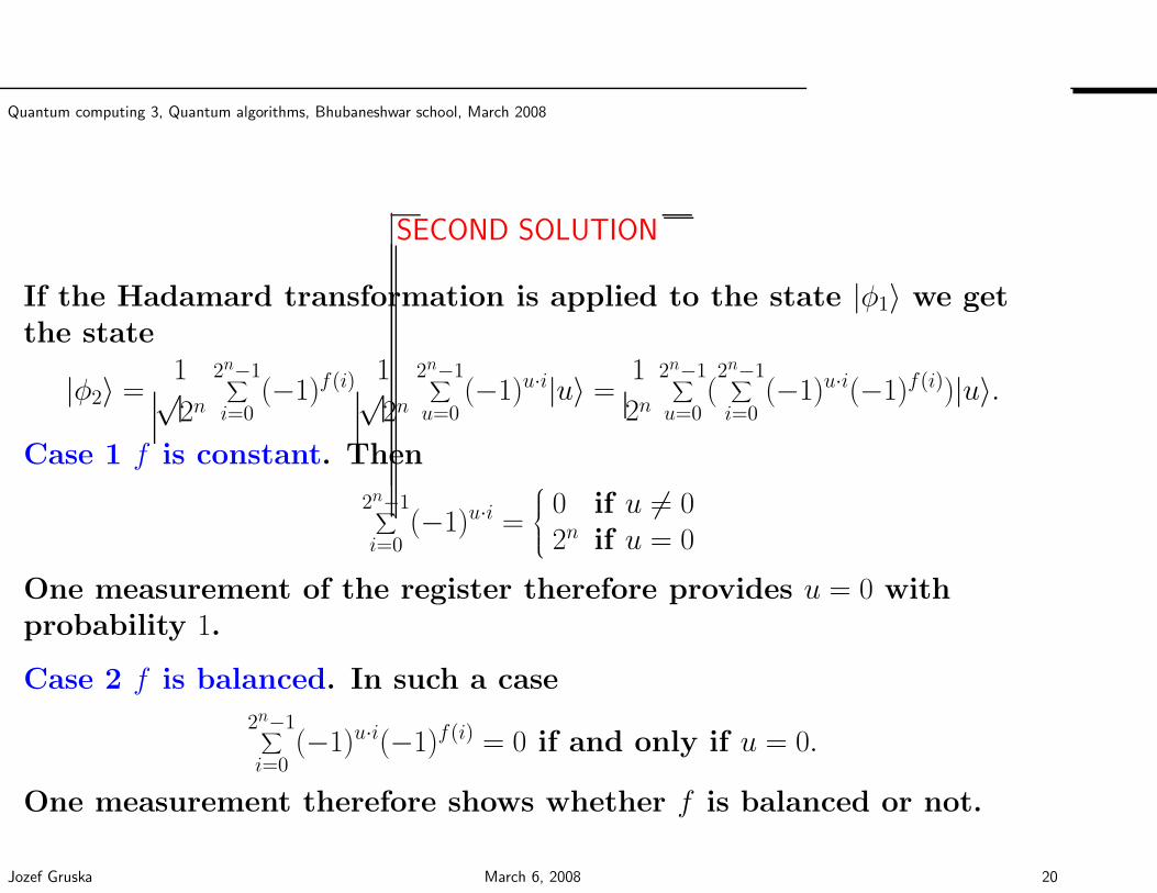
Quantum computing 3, Quantum algorithms, Bhubaneshwar school, March 2008
SECOND SOLUTION
If the Hadamard transformation is applied to the state |φ1〉 we getthe state
|φ2〉 =1√2n
2n−1∑
i=0(−1)f(i) 1√
2n2n−1∑
u=0(−1)u·i|u〉 =
1
2n2n−1∑
u=0(2n−1∑
i=0(−1)u·i(−1)f(i))|u〉.
Case 1 f is constant. Then
2n−1∑
i=0(−1)u·i =
0 if u 6= 02n if u = 0
One measurement of the register therefore provides u = 0 withprobability 1.
Case 2 f is balanced. In such a case
2n−1∑
i=0(−1)u·i(−1)f(i) = 0 if and only if u = 0.
One measurement therefore shows whether f is balanced or not.
Jozef Gruska March 6, 2008 20
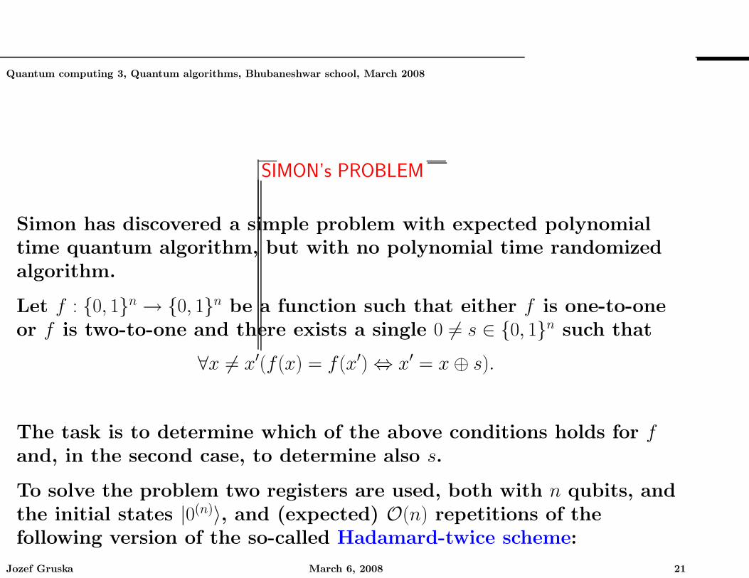
Quantum computing 3, Quantum algorithms, Bhubaneshwar school, March 2008
SIMON’s PROBLEM
Simon has discovered a simple problem with expected polynomialtime quantum algorithm, but with no polynomial time randomizedalgorithm.
Let f : 0, 1n → 0, 1n be a function such that either f is one-to-oneor f is two-to-one and there exists a single 0 6= s ∈ 0, 1n such that
∀x 6= x′(f(x) = f(x′) ⇔ x′ = x⊕ s).
The task is to determine which of the above conditions holds for fand, in the second case, to determine also s.
To solve the problem two registers are used, both with n qubits, andthe initial states |0(n)〉, and (expected) O(n) repetitions of thefollowing version of the so-called Hadamard-twice scheme:
Jozef Gruska March 6, 2008 21
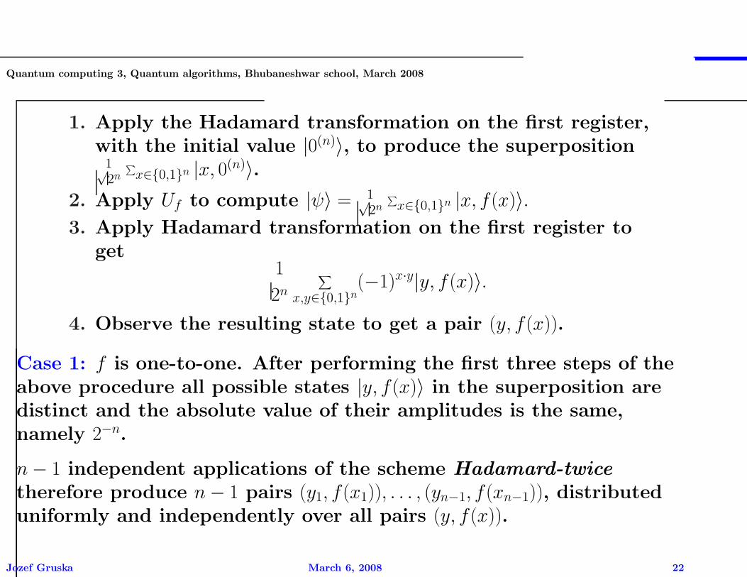
Quantum computing 3, Quantum algorithms, Bhubaneshwar school, March 2008
1. Apply the Hadamard transformation on the first register,with the initial value |0(n)〉, to produce the superposition
1√2n
∑
x∈0,1n |x, 0(n)〉.2. Apply Uf to compute |ψ〉 = 1√
2n∑
x∈0,1n |x, f(x)〉.3. Apply Hadamard transformation on the first register to
get1
2n∑
x,y∈0,1n(−1)x·y|y, f(x)〉.
4. Observe the resulting state to get a pair (y, f(x)).
Case 1: f is one-to-one. After performing the first three steps of theabove procedure all possible states |y, f(x)〉 in the superposition aredistinct and the absolute value of their amplitudes is the same,namely 2−n.
n− 1 independent applications of the scheme Hadamard-twice
therefore produce n− 1 pairs (y1, f(x1)), . . . , (yn−1, f(xn−1)), distributeduniformly and independently over all pairs (y, f(x)).
Jozef Gruska March 6, 2008 22
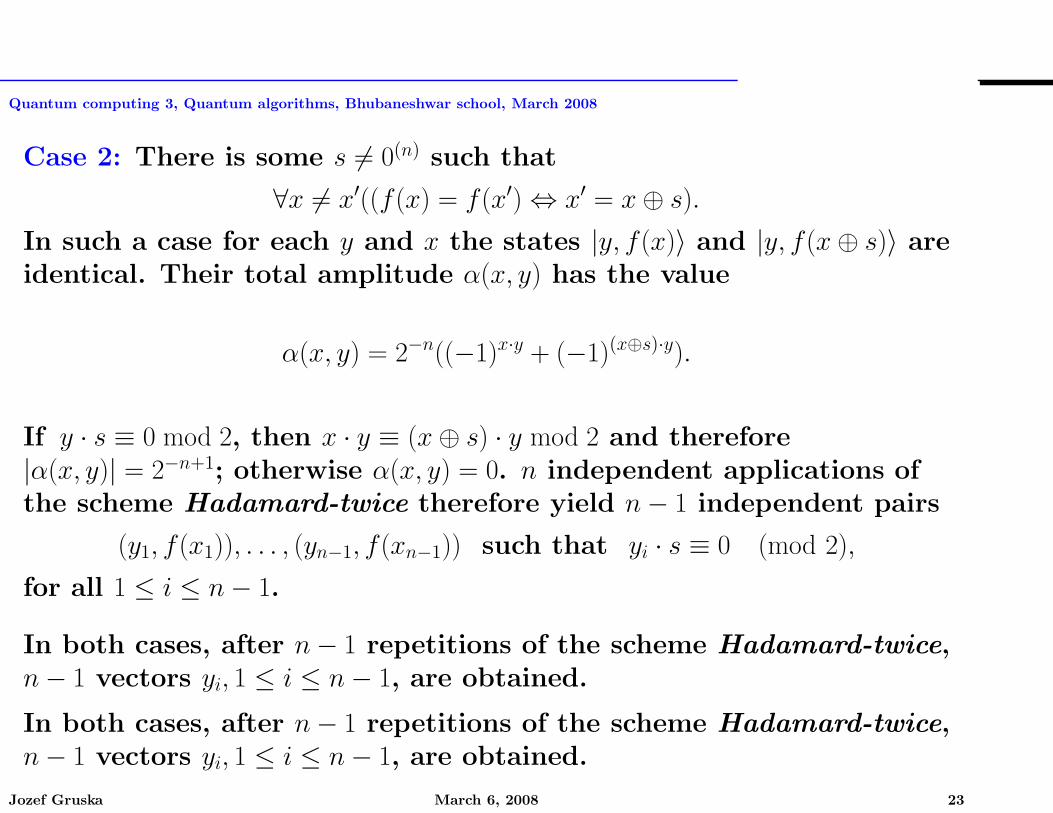
Quantum computing 3, Quantum algorithms, Bhubaneshwar school, March 2008
Case 2: There is some s 6= 0(n) such that
∀x 6= x′((f(x) = f(x′) ⇔ x′ = x⊕ s).
In such a case for each y and x the states |y, f(x)〉 and |y, f(x⊕ s)〉 areidentical. Their total amplitude α(x, y) has the value
α(x, y) = 2−n((−1)x·y + (−1)(x⊕s)·y).
If y · s ≡ 0 mod 2, then x · y ≡ (x⊕ s) · y mod 2 and therefore|α(x, y)| = 2−n+1; otherwise α(x, y) = 0. n independent applications ofthe scheme Hadamard-twice therefore yield n− 1 independent pairs
(y1, f(x1)), . . . , (yn−1, f(xn−1)) such that yi · s ≡ 0 (mod 2),
for all 1 ≤ i ≤ n− 1.
In both cases, after n− 1 repetitions of the scheme Hadamard-twice,n− 1 vectors yi, 1 ≤ i ≤ n− 1, are obtained.
In both cases, after n− 1 repetitions of the scheme Hadamard-twice,n− 1 vectors yi, 1 ≤ i ≤ n− 1, are obtained.
Jozef Gruska March 6, 2008 23
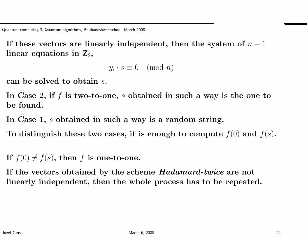
Quantum computing 3, Quantum algorithms, Bhubaneshwar school, March 2008
If these vectors are linearly independent, then the system of n− 1linear equations in Z2,
yi · s ≡ 0 (mod n)
can be solved to obtain s.
In Case 2, if f is two-to-one, s obtained in such a way is the one tobe found.
In Case 1, s obtained in such a way is a random string.
To distinguish these two cases, it is enough to compute f(0) and f(s).
If f(0) 6= f(s), then f is one-to-one.
If the vectors obtained by the scheme Hadamard-twice are notlinearly independent, then the whole process has to be repeated.
Jozef Gruska March 6, 2008 24
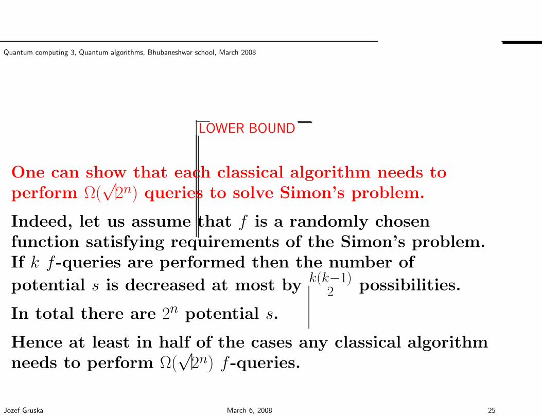
Quantum computing 3, Quantum algorithms, Bhubaneshwar school, March 2008
LOWER BOUND
One can show that each classical algorithm needs toperform Ω(
√2n) queries to solve Simon’s problem.
Indeed, let us assume that f is a randomly chosenfunction satisfying requirements of the Simon’s problem.If k f-queries are performed then the number of
potential s is decreased at most by k(k−1)2 possibilities.
In total there are 2n potential s.
Hence at least in half of the cases any classical algorithmneeds to perform Ω(
√2n) f-queries.
Jozef Gruska March 6, 2008 25
Quantum computing 3, Quantum algorithms, Bhubaneshwar school, March 2008
QUANTUM FOURIER TRANSFORM and SHOR’s ALGORITHMS
Perhaps the most significant success of quantum computing so farhas been Shor’s polynomial time algorithm for factorization to bepresented in this section. This is a highly nontrivial algorithm thatuses a new technique, that of Quantum Fourier Transform, that willalso be illustrated in this chapter.
The fastest classical algorithm to factor m bit numbers requires time
O(ecm1/3(lgm)2/3).
Shor’s factorization algorithm requires O(m2 lg2m lg lgm) time on aquantum computer and polynomial time on a classical computer.
Of interest and importance is also another Shor’s polynomial timealgorithm for discrete logarithm to be also presented in this chapter.
Correctness and efficiency of Shor’s algorithm is based on severalsimple results from number theory to be presented first.
Jozef Gruska March 6, 2008 26
Quantum computing 3, Quantum algorithms, Bhubaneshwar school, March 2008
BASICS
• Modulo operation: Given two integers n > m, then
n mod m
is the remmainder we get when n is divided by m.
Example: 24 mod 8 = 0; 24 mod 7 = 3; 24 mod 6 = 0;24 mod 5 = 4.
Useful facts
a · b mod n = ((a mod n) · (b mod n)) mod n
ab mod n = ((a mod n)b) mod n
Class work: Compute 3123456789 mod 26 =???Jozef Gruska March 6, 2008 27
Quantum computing 3, Quantum algorithms, Bhubaneshwar school, March 2008
• For three integers a, b and n we define
a ≡ b(modn)
if(a− b) mod n = 0
Examples 4 ≡ 11(mod15).
• Greatest common divisor Given integers n,m we denote by
gcd(n,m)
the gretaest common divisor of m and n.
Examples; gcd(21, 91) = 7; gcd(51, 204) =??
Useful fact 1 Already Euklid new a simple algorithm to computegreatest common divisor of arbitrary two integers.
Useful fact 2 For any integers n, a, b there are integers x, y such that
ax + by = gcd(a, b) mod n
Jozef Gruska March 6, 2008 28
Quantum computing 3, Quantum algorithms, Bhubaneshwar school, March 2008
FIRST REDUCTION
Lemma 0.1 If there is a polynomial time deterministic (randomized) [quantum]algorithm to find a nontrivial solution of the modular quadratic equations
a2 ≡ 1 (mod n),
then there is a polynomial time deterministic (randomized) [quantum] algorithm tofactorize integers.
Proof. Let a 6= ±1 be such that a2 ≡ 1 (mod n). Since
a2 − 1 = (a + 1)(a− 1),
if n is not prime, then a prime factor of n has to be a prime factor of either a + 1 ora− 1.
By using Euclid’s algorithm to compute
gcd(a + 1, n) and gcd(a− 1, n)
we can find, in O(lg n) steps, a prime factor of n.
Jozef Gruska March 6, 2008 29
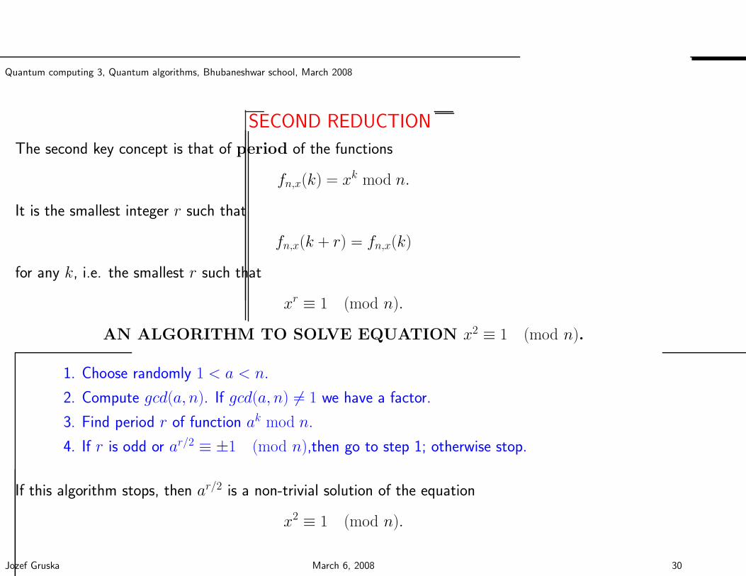
Quantum computing 3, Quantum algorithms, Bhubaneshwar school, March 2008
SECOND REDUCTION
The second key concept is that of period of the functions
fn,x(k) = xk mod n.
It is the smallest integer r such that
fn,x(k + r) = fn,x(k)
for any k, i.e. the smallest r such that
xr ≡ 1 (mod n).
AN ALGORITHM TO SOLVE EQUATION x2 ≡ 1 (mod n).
1. Choose randomly 1 < a < n.
2. Compute gcd(a, n). If gcd(a, n) 6= 1 we have a factor.
3. Find period r of function ak mod n.
4. If r is odd or ar/2 ≡ ±1 (mod n),then go to step 1; otherwise stop.
If this algorithm stops, then ar/2 is a non-trivial solution of the equation
x2 ≡ 1 (mod n).
Jozef Gruska March 6, 2008 30
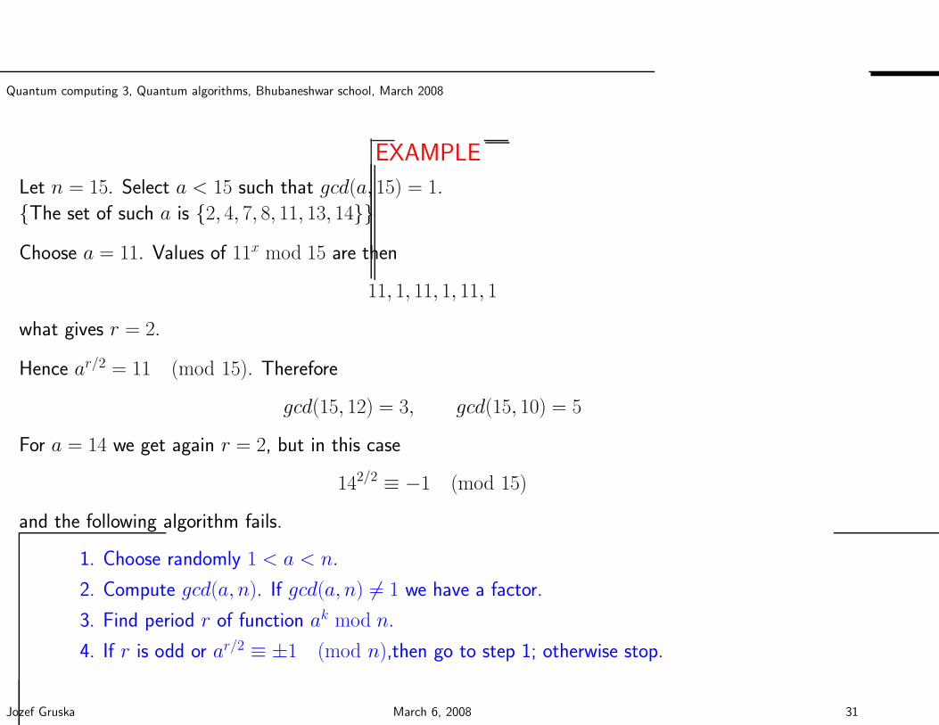
Quantum computing 3, Quantum algorithms, Bhubaneshwar school, March 2008
EXAMPLE
Let n = 15. Select a < 15 such that gcd(a, 15) = 1.
The set of such a is 2, 4, 7, 8, 11, 13, 14
Choose a = 11. Values of 11x mod 15 are then
11, 1, 11, 1, 11, 1
what gives r = 2.
Hence ar/2 = 11 (mod 15). Therefore
gcd(15, 12) = 3, gcd(15, 10) = 5
For a = 14 we get again r = 2, but in this case
142/2 ≡ −1 (mod 15)
and the following algorithm fails.
1. Choose randomly 1 < a < n.
2. Compute gcd(a, n). If gcd(a, n) 6= 1 we have a factor.
3. Find period r of function ak mod n.
4. If r is odd or ar/2 ≡ ±1 (mod n),then go to step 1; otherwise stop.
Jozef Gruska March 6, 2008 31
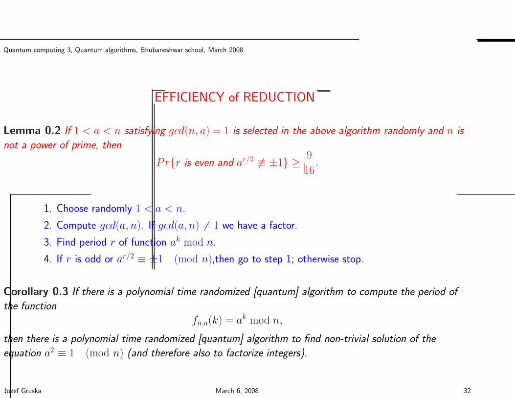
Quantum computing 3, Quantum algorithms, Bhubaneshwar school, March 2008
EFFICIENCY of REDUCTION
Lemma 0.2 If 1 < a < n satisfying gcd(n, a) = 1 is selected in the above algorithm randomly and n is
not a power of prime, then
Prr is even and ar/2 6≡ ±1 ≥ 9
16.
1. Choose randomly 1 < a < n.
2. Compute gcd(a, n). If gcd(a, n) 6= 1 we have a factor.
3. Find period r of function ak mod n.
4. If r is odd or ar/2 ≡ ±1 (mod n),then go to step 1; otherwise stop.
Corollary 0.3 If there is a polynomial time randomized [quantum] algorithm to compute the period of
the function
fn,a(k) = ak mod n,
then there is a polynomial time randomized [quantum] algorithm to find non-trivial solution of the
equation a2 ≡ 1 (mod n) (and therefore also to factorize integers).
Jozef Gruska March 6, 2008 32
Quantum computing 3, Quantum algorithms, Bhubaneshwar school, March 2008
A GENERAL SCHEME FOR SHOR’S ALGORITHM
Jozef Gruska March 6, 2008 33
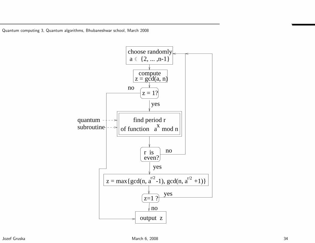
Quantum computing 3, Quantum algorithms, Bhubaneshwar school, March 2008
quantumx
find period rsubroutine
r iseven?
r/2 r/2
z=1 ?
output z
no
yes
no
computez = gcd(a, n)
z = 1?
yes
no
z = maxgcd(n, a -1), gcd(n, a +1)
yes
of function a mod n
choose randomlya 2, ... ,n-1
Jozef Gruska March 6, 2008 34
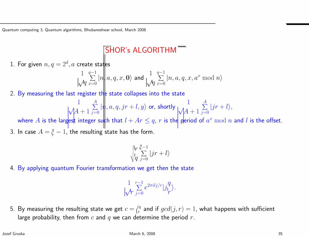
Quantum computing 3, Quantum algorithms, Bhubaneshwar school, March 2008
SHOR’s ALGORITHM
1. For given n, q = 2d, a create states
1√q
q−1∑
x=0|n, a, q, x,0〉 and
1√q
q−1∑
x=0|n, a, q, x, ax mod n〉
2. By measuring the last register the state collapses into the state
1√A + 1
A∑
j=0|n, a, q, jr + l, y〉 or, shortly
1√A + 1
A∑
j=0|jr + l〉,
where A is the largest integer such that l + Ar ≤ q, r is the period of ax mod n and l is the offset.
3. In case A = qr− 1, the resulting state has the form.
√√√√√
r
q
qr−1∑
j=0|jr + l〉
4. By applying quantum Fourier transformation we get then the state
1√r
r−1∑
j=0e2πilj/r|jq
r〉.
5. By measuring the resulting state we get c = jqr and if gcd(j, r) = 1, what happens with sufficient
large probability, then from c and q we can determine the period r.
Jozef Gruska March 6, 2008 35
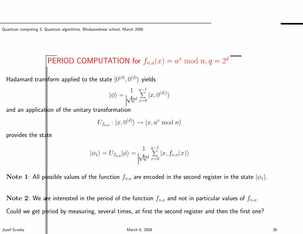
Quantum computing 3, Quantum algorithms, Bhubaneshwar school, March 2008
PERIOD COMPUTATION for fn,a(x) = ax mod n, q = 2d
Hadamard transform applied to the state |0(d), 0(d)〉 yields
|φ〉 =1√2d
q−1∑
x=0|x, 0(d))〉
and an application of the unitary transformation
Ufn,a : |x, 0(d)〉 → |x, ax mod n〉
provides the state
|φ1〉 = Ufn,a|φ〉 =1√2d
q−1∑
x=0|x, fn,a(x)〉
Note 1: All possible values of the function fn,a are encoded in the second register in the state |φ1〉.
Note 2: We are interested in the period of the function fn,a and not in particular values of fn,a.
Could we get period by measuring, several times, at first the second register and then the first one?
Jozef Gruska March 6, 2008 36
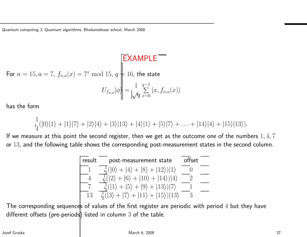
Quantum computing 3, Quantum algorithms, Bhubaneshwar school, March 2008
EXAMPLE
For n = 15, a = 7, fn,a(x) = 7x mod 15, q = 16, the state
Ufn,a|φ〉 =1√q
q−1∑
x=0|x, fn,a(x)〉
has the form
1
4(|0〉|1〉 + |1〉|7〉 + |2〉|4〉 + |3〉|13〉 + |4〉|1〉 + |5〉|7〉 + . . . + |14〉|4〉 + |15〉|13〉).
If we measure at this point the second register, then we get as the outcome one of the numbers 1, 4, 7
or 13, and the following table shows the corresponding post-measurement states in the second column.
result post-measurement state offset
1 12(|0〉 + |4〉 + |8〉 + |12〉)|1〉 0
4 12(|2〉 + |6〉 + |10〉 + |14〉)|4〉 2
7 12(|1〉 + |5〉 + |9〉 + |13〉)|7〉 1
13 12(|3〉 + |7〉 + |11〉 + |15〉)|13〉 3
The corresponding sequences of values of the first register are periodic with period 4 but they have
different offsets (pre-periods) listed in column 3 of the table.
Jozef Gruska March 6, 2008 37
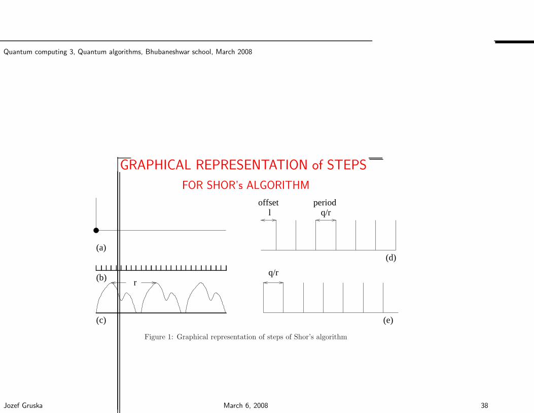
Quantum computing 3, Quantum algorithms, Bhubaneshwar school, March 2008
GRAPHICAL REPRESENTATION of STEPS
FOR SHOR’s ALGORITHM
q/r
(e)
q/r
(a)(d)
period
(b)
(c)
r
loffset
Figure 1: Graphical representation of steps of Shor’s algorithm
Jozef Gruska March 6, 2008 38
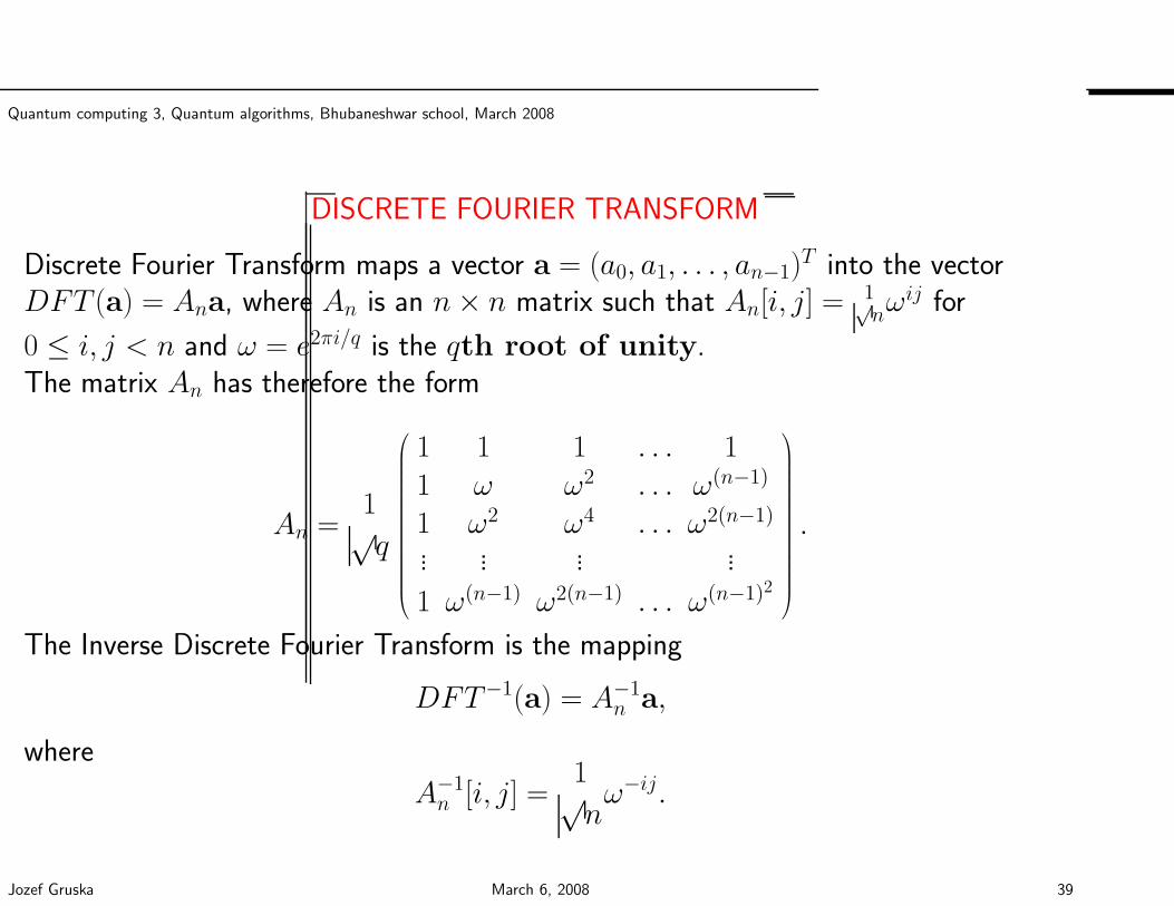
Quantum computing 3, Quantum algorithms, Bhubaneshwar school, March 2008
DISCRETE FOURIER TRANSFORM
Discrete Fourier Transform maps a vector a = (a0, a1, . . . , an−1)T into the vector
DFT (a) = Ana, where An is an n× n matrix such that An[i, j] = 1√nω
ij for
0 ≤ i, j < n and ω = e2πi/q is the qth root of unity.The matrix An has therefore the form
An =1√q
1 1 1 . . . 11 ω ω2 . . . ω(n−1)
1 ω2 ω4 . . . ω2(n−1)
... ... ... ...
1 ω(n−1) ω2(n−1) . . . ω(n−1)2
.
The Inverse Discrete Fourier Transform is the mapping
DFT−1(a) = A−1n a,
where
A−1n [i, j] =
1√nω−ij.
Jozef Gruska March 6, 2008 39
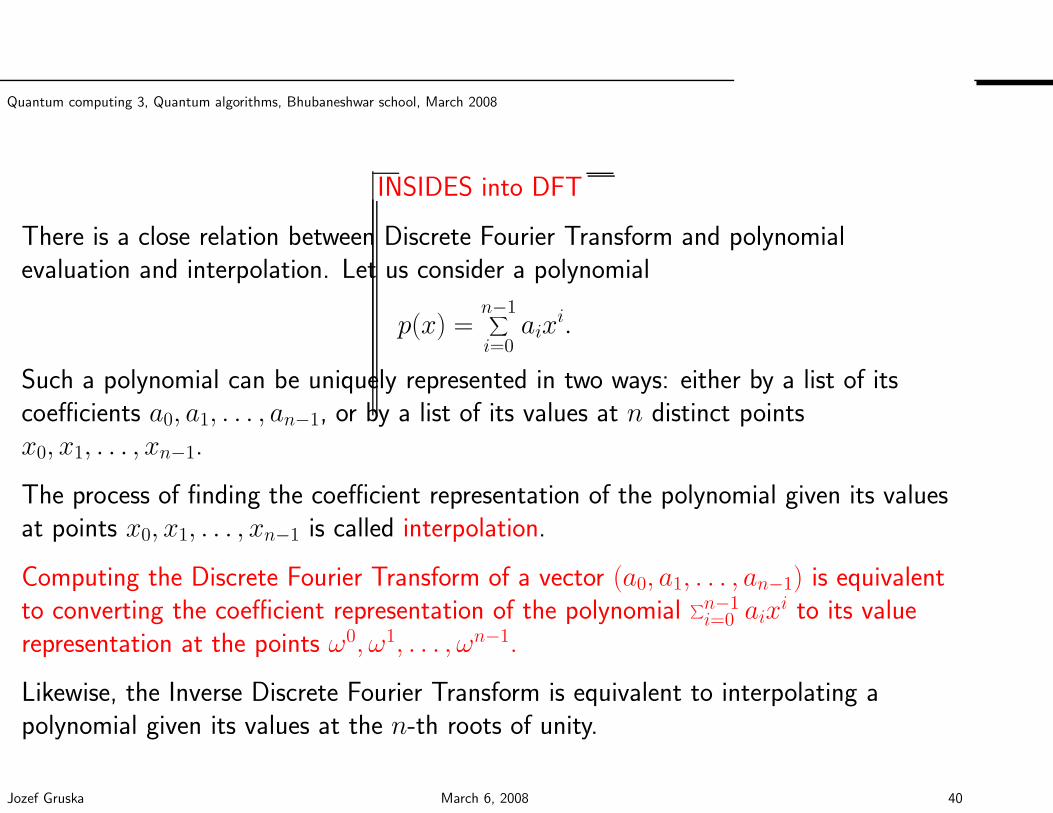
Quantum computing 3, Quantum algorithms, Bhubaneshwar school, March 2008
INSIDES into DFT
There is a close relation between Discrete Fourier Transform and polynomialevaluation and interpolation. Let us consider a polynomial
p(x) =n−1∑
i=0aix
i.
Such a polynomial can be uniquely represented in two ways: either by a list of itscoefficients a0, a1, . . . , an−1, or by a list of its values at n distinct pointsx0, x1, . . . , xn−1.
The process of finding the coefficient representation of the polynomial given its valuesat points x0, x1, . . . , xn−1 is called interpolation.
Computing the Discrete Fourier Transform of a vector (a0, a1, . . . , an−1) is equivalentto converting the coefficient representation of the polynomial ∑n−1
i=0 aixi to its value
representation at the points ω0, ω1, . . . , ωn−1.
Likewise, the Inverse Discrete Fourier Transform is equivalent to interpolating apolynomial given its values at the n-th roots of unity.
Jozef Gruska March 6, 2008 40
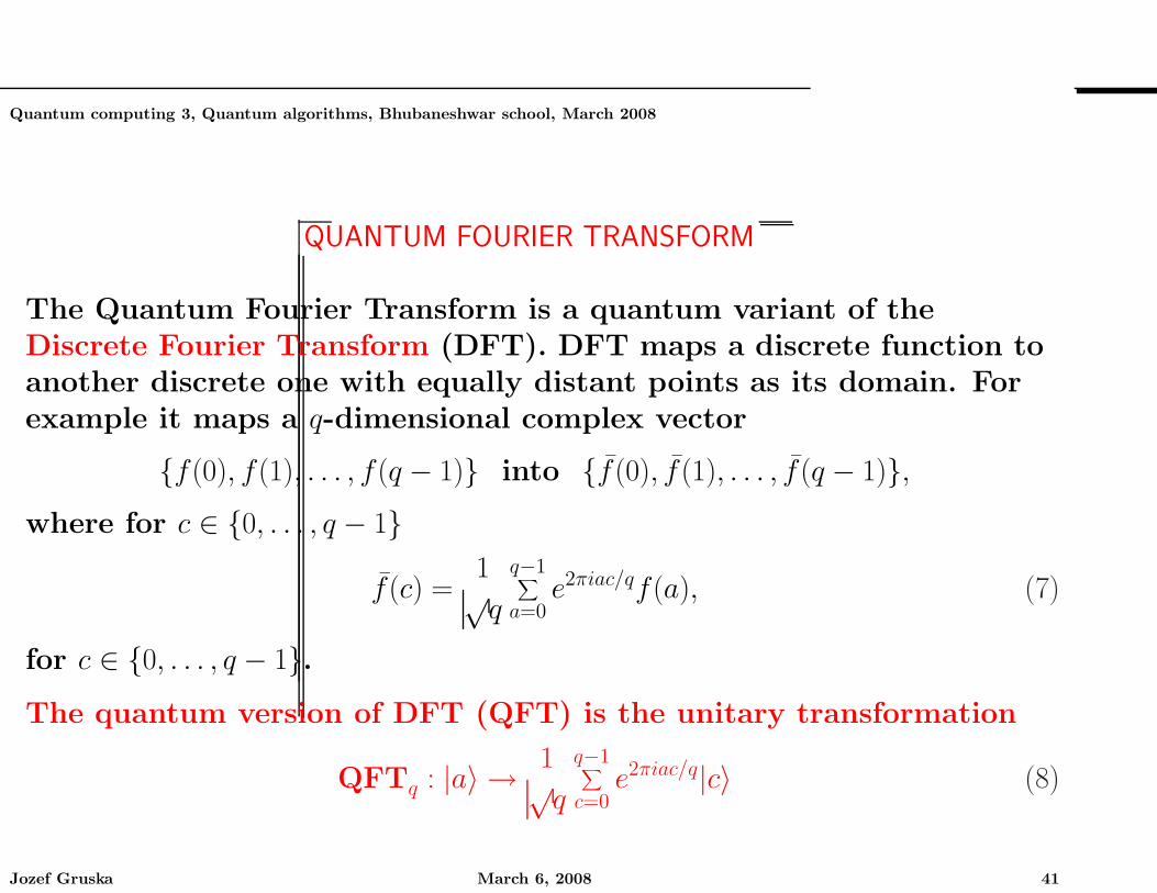
Quantum computing 3, Quantum algorithms, Bhubaneshwar school, March 2008
QUANTUM FOURIER TRANSFORM
The Quantum Fourier Transform is a quantum variant of theDiscrete Fourier Transform (DFT). DFT maps a discrete function toanother discrete one with equally distant points as its domain. Forexample it maps a q-dimensional complex vector
f(0), f(1), . . . , f(q − 1) into f (0), f (1), . . . , f (q − 1),where for c ∈ 0, . . . , q − 1
f(c) =1√q
q−1∑
a=0e2πiac/qf(a), (7)
for c ∈ 0, . . . , q − 1.The quantum version of DFT (QFT) is the unitary transformation
QFTq : |a〉 → 1√q
q−1∑
c=0e2πiac/q|c〉 (8)
Jozef Gruska March 6, 2008 41
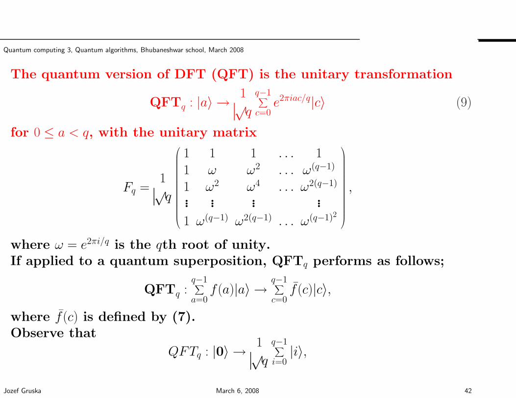
Quantum computing 3, Quantum algorithms, Bhubaneshwar school, March 2008
The quantum version of DFT (QFT) is the unitary transformation
QFTq : |a〉 → 1√q
q−1∑
c=0e2πiac/q|c〉 (9)
for 0 ≤ a < q, with the unitary matrix
Fq =1√q
1 1 1 . . . 11 ω ω2 . . . ω(q−1)
1 ω2 ω4 . . . ω2(q−1)
... ... ... ...
1 ω(q−1) ω2(q−1) . . . ω(q−1)2
,
where ω = e2πi/q is the qth root of unity.If applied to a quantum superposition, QFTq performs as follows;
QFTq :q−1∑
a=0f(a)|a〉 →
q−1∑
c=0f (c)|c〉,
where f(c) is defined by (7).Observe that
QFTq : |0〉 → 1√q
q−1∑
i=0|i〉,
Jozef Gruska March 6, 2008 42
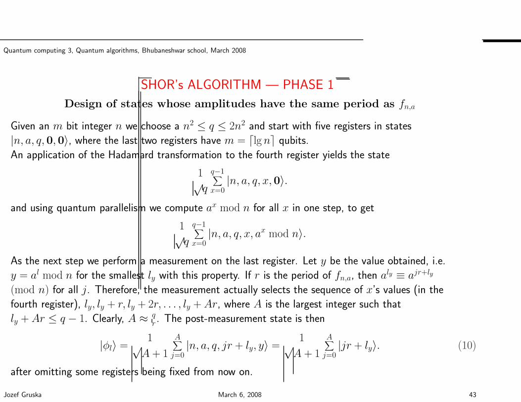
Quantum computing 3, Quantum algorithms, Bhubaneshwar school, March 2008
SHOR’s ALGORITHM — PHASE 1
Design of states whose amplitudes have the same period as fn,a
Given an m bit integer n we choose a n2 ≤ q ≤ 2n2 and start with five registers in states
|n, a, q,0,0〉, where the last two registers have m = ⌈lgn⌉ qubits.
An application of the Hadamard transformation to the fourth register yields the state
1√q
q−1∑
x=0|n, a, q, x,0〉.
and using quantum parallelism we compute ax mod n for all x in one step, to get
1√q
q−1∑
x=0|n, a, q, x, ax mod n〉.
As the next step we perform a measurement on the last register. Let y be the value obtained, i.e.
y = al mod n for the smallest ly with this property. If r is the period of fn,a, then aly ≡ ajr+ly
(mod n) for all j. Therefore, the measurement actually selects the sequence of x’s values (in the
fourth register), ly, ly + r, ly + 2r, . . . , ly + Ar, where A is the largest integer such that
ly + Ar ≤ q − 1. Clearly, A ≈ qr . The post-measurement state is then
|φl〉 =1√A + 1
A∑
j=0|n, a, q, jr + ly, y〉 =
1√A + 1
A∑
j=0|jr + ly〉. (10)
after omitting some registers being fixed from now on.
Jozef Gruska March 6, 2008 43
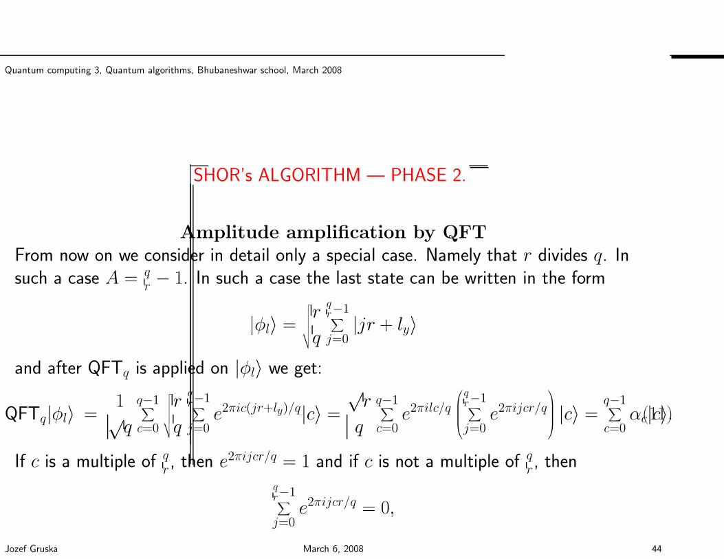
Quantum computing 3, Quantum algorithms, Bhubaneshwar school, March 2008
SHOR’s ALGORITHM — PHASE 2.
Amplitude amplification by QFTFrom now on we consider in detail only a special case. Namely that r divides q. Insuch a case A = q
r − 1. In such a case the last state can be written in the form
|φl〉 =
√√√√√√
r
q
qr−1∑
j=0|jr + ly〉
and after QFTq is applied on |φl〉 we get:
QFTq|φl〉 =1√q
q−1∑
c=0
√√√√√√
r
q
qr−1∑
j=0e2πic(jr+ly)/q|c〉 =
√r
q
q−1∑
c=0e2πilc/q
qr−1∑
j=0e2πijcr/q
|c〉 =
q−1∑
c=0αc|c〉.(11)
If c is a multiple of qr, then e2πijcr/q = 1 and if c is not a multiple of q
r , thenqr−1∑
j=0e2πijcr/q = 0,
Jozef Gruska March 6, 2008 44
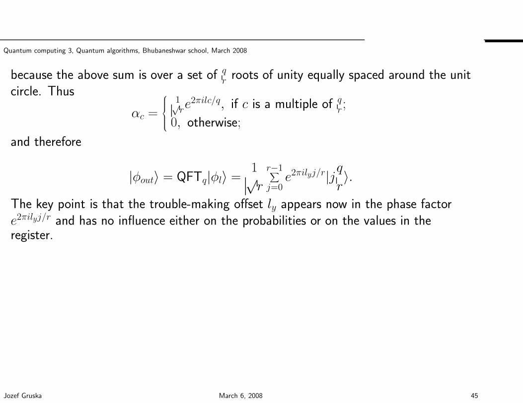
Quantum computing 3, Quantum algorithms, Bhubaneshwar school, March 2008
because the above sum is over a set of qr roots of unity equally spaced around the unit
circle. Thus
αc =
1√re
2πilc/q, if c is a multiple of qr ;
0, otherwise;
and therefore
|φout〉 = QFTq|φl〉 =1√r
r−1∑
j=0e2πilyj/r|jq
r〉.
The key point is that the trouble-making offset ly appears now in the phase factore2πilyj/r and has no influence either on the probabilities or on the values in theregister.
Jozef Gruska March 6, 2008 45
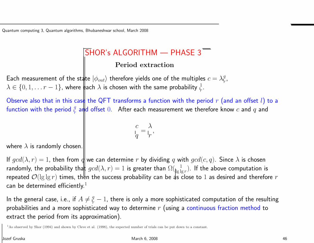
Quantum computing 3, Quantum algorithms, Bhubaneshwar school, March 2008
SHOR’s ALGORITHM — PHASE 3
Period extraction
Each measurement of the state |φout〉 therefore yields one of the multiples c = λqr,
λ ∈ 0, 1, . . . r − 1, where each λ is chosen with the same probability 1r .
Observe also that in this case the QFT transforms a function with the period r (and an offset l) to a
function with the period qr and offset 0. After each measurement we therefore know c and q and
c
q=λ
r,
where λ is randomly chosen.
If gcd(λ, r) = 1, then from q we can determine r by dividing q with gcd(c, q). Since λ is chosen
randomly, the probability that gcd(λ, r) = 1 is greater than Ω( 1lg lg r). If the above computation is
repeated O(lg lg r) times, then the success probability can be as close to 1 as desired and therefore r
can be determined efficiently.1
In the general case, i.e., if A 6= qr− 1, there is only a more sophisticated computation of the resulting
probabilities and a more sophisticated way to determine r (using a continuous fraction method to
extract the period from its approximation).1As observed by Shor (1994) and shown by Cleve et al. (1998), the expected number of trials can be put down to a constant.
Jozef Gruska March 6, 2008 46
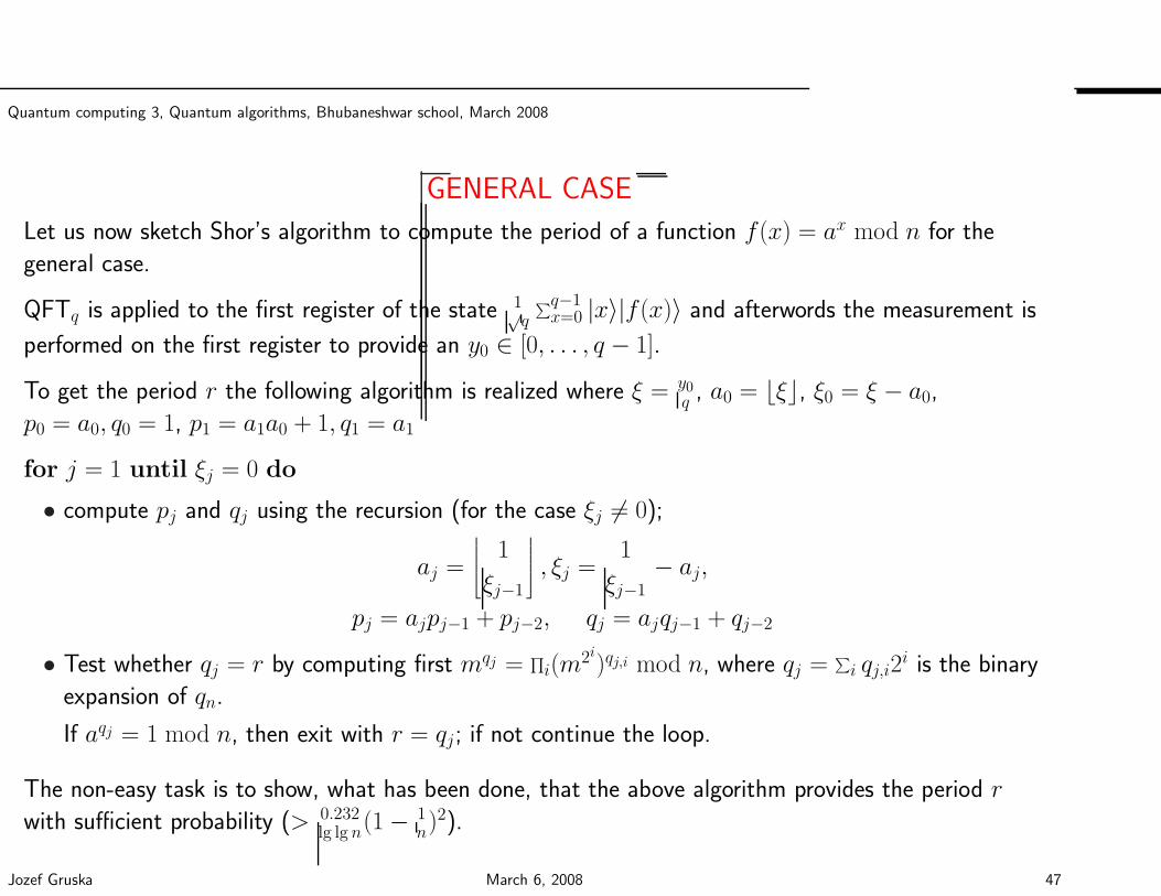
Quantum computing 3, Quantum algorithms, Bhubaneshwar school, March 2008
GENERAL CASE
Let us now sketch Shor’s algorithm to compute the period of a function f(x) = ax mod n for the
general case.
QFTq is applied to the first register of the state 1√q
∑q−1x=0 |x〉|f(x)〉 and afterwords the measurement is
performed on the first register to provide an y0 ∈ [0, . . . , q − 1].
To get the period r the following algorithm is realized where ξ = y0q, a0 = ⌊ξ⌋, ξ0 = ξ − a0,
p0 = a0, q0 = 1, p1 = a1a0 + 1, q1 = a1
for j = 1 until ξj = 0 do
• compute pj and qj using the recursion (for the case ξj 6= 0);
aj =
1
ξj−1
, ξj =
1
ξj−1− aj,
pj = ajpj−1 + pj−2, qj = ajqj−1 + qj−2
• Test whether qj = r by computing first mqj =∏
i(m2i)qj,i mod n, where qj =
∑
i qj,i2i is the binary
expansion of qn.
If aqj = 1 mod n, then exit with r = qj; if not continue the loop.
The non-easy task is to show, what has been done, that the above algorithm provides the period r
with sufficient probability (> 0.232lg lg n(1 − 1
n)2).
Jozef Gruska March 6, 2008 47
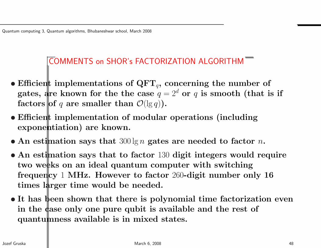
Quantum computing 3, Quantum algorithms, Bhubaneshwar school, March 2008
COMMENTS on SHOR’s FACTORIZATION ALGORITHM
• Efficient implementations of QFTq, concerning the number ofgates, are known for the the case q = 2d or q is smooth (that is iffactors of q are smaller than O(lg q)).
• Efficient implementation of modular operations (includingexponentiation) are known.
• An estimation says that 300 lg n gates are needed to factor n.
• An estimation says that to factor 130 digit integers would requiretwo weeks on an ideal quantum computer with switchingfrequency 1 MHz. However to factor 260-digit number only 16times larger time would be needed.
• It has been shown that there is polynomial time factorization evenin the case only one pure qubit is available and the rest ofquantumness available is in mixed states.
Jozef Gruska March 6, 2008 48
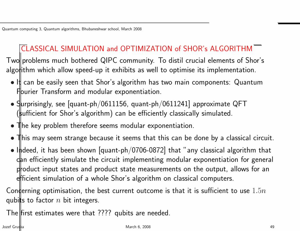
Quantum computing 3, Quantum algorithms, Bhubaneshwar school, March 2008
CLASSICAL SIMULATION and OPTIMIZATION of SHOR’s ALGORITHM
Two problems much bothered QIPC community. To distil crucial elements of Shor’salgorithm which allow speed-up it exhibits as well to optimise its implementation.
• It can be easily seen that Shor’s algorithm has two main components: QuantumFourier Transform and modular exponentiation.
• Surprisingly, see [quant-ph/0611156, quant-ph/0611241] approximate QFT(sufficient for Shor’s algorithm) can be efficiently classically simulated.
• The key problem therefore seems modular exponentiation.
• This may seem strange because it seems that this can be done by a classical circuit.
• Indeed, it has been shown [quant-ph/0706-0872] that ”any classical algorithm thatcan efficiently simulate the circuit implementing modular exponentiation for generalproduct input states and product state measurements on the output, allows for anefficient simulation of a whole Shor’s algorithm on classical computers.
Concerning optimisation, the best current outcome is that it is sufficient to use 1.5nqubits to factor n bit integers.
The first estimates were that ???? qubits are needed.
Jozef Gruska March 6, 2008 49
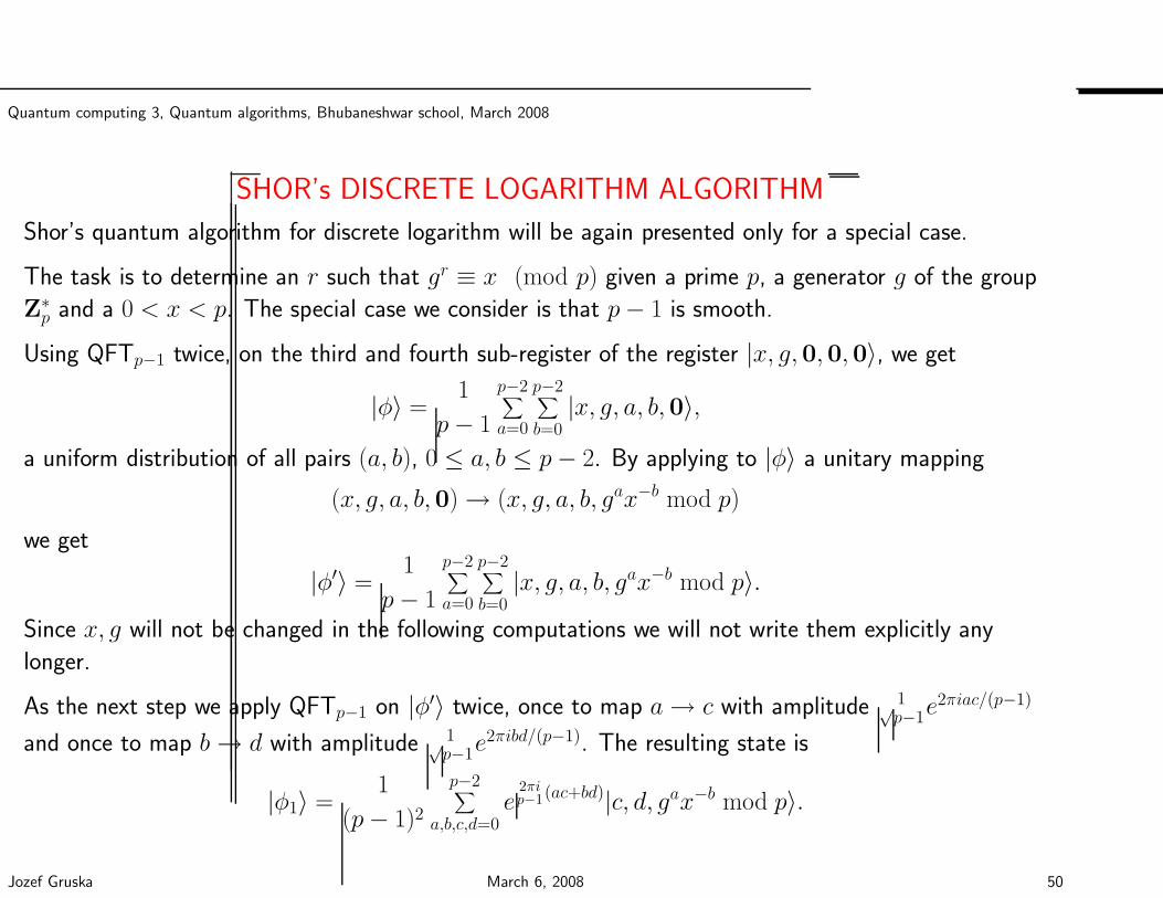
Quantum computing 3, Quantum algorithms, Bhubaneshwar school, March 2008
SHOR’s DISCRETE LOGARITHM ALGORITHM
Shor’s quantum algorithm for discrete logarithm will be again presented only for a special case.
The task is to determine an r such that gr ≡ x (mod p) given a prime p, a generator g of the group
Z∗p and a 0 < x < p. The special case we consider is that p− 1 is smooth.
Using QFTp−1 twice, on the third and fourth sub-register of the register |x, g,0,0,0〉, we get
|φ〉 =1
p− 1
p−2∑
a=0
p−2∑
b=0|x, g, a, b,0〉,
a uniform distribution of all pairs (a, b), 0 ≤ a, b ≤ p− 2. By applying to |φ〉 a unitary mapping
(x, g, a, b,0) → (x, g, a, b, gax−b mod p)
we get
|φ′〉 =1
p− 1
p−2∑
a=0
p−2∑
b=0|x, g, a, b, gax−b mod p〉.
Since x, g will not be changed in the following computations we will not write them explicitly any
longer.
As the next step we apply QFTp−1 on |φ′〉 twice, once to map a→ c with amplitude 1√p−1e
2πiac/(p−1)
and once to map b→ d with amplitude 1√p−1e
2πibd/(p−1). The resulting state is
|φ1〉 =1
(p− 1)2
p−2∑
a,b,c,d=0e
2πip−1(ac+bd)|c, d, gax−b mod p〉.
Jozef Gruska March 6, 2008 50
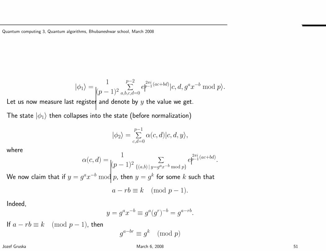
Quantum computing 3, Quantum algorithms, Bhubaneshwar school, March 2008
|φ1〉 =1
(p− 1)2
p−2∑
a,b,c,d=0e
2πip−1(ac+bd)|c, d, gax−b mod p〉.
Let us now measure last register and denote by y the value we get.
The state |φ1〉 then collapses into the state (before normalization)
|φ2〉 =p−1∑
c,d=0α(c, d)|c, d, y〉,
where
α(c, d) =1
(p− 1)2∑
(a,b) | y=gax−b mod pe
2πip−1(ac+bd).
We now claim that if y = gax−b mod p, then y = gk for some k such that
a− rb ≡ k (mod p− 1).
Indeed,
y = gax−b ≡ ga(gr)−b = ga−rb.
If a− rb ≡ k (mod p− 1), then
ga−br ≡ gk (mod p)
Jozef Gruska March 6, 2008 51
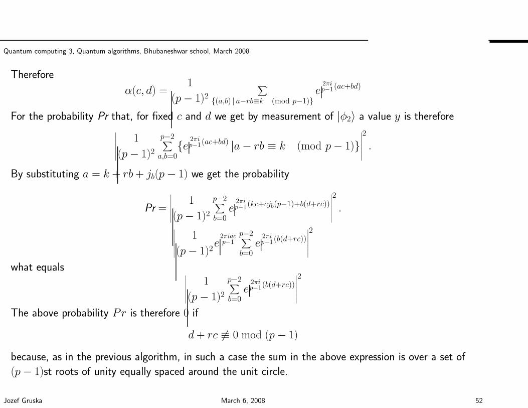
Quantum computing 3, Quantum algorithms, Bhubaneshwar school, March 2008
Therefore
α(c, d) =1
(p− 1)2∑
(a,b) | a−rb≡k (mod p−1)e
2πip−1(ac+bd)
For the probability Pr that, for fixed c and d we get by measurement of |φ2〉 a value y is therefore∣∣∣∣∣∣∣
1
(p− 1)2
p−2∑
a,b=0e 2πi
p−1(ac+bd) |a− rb ≡ k (mod p− 1)∣∣∣∣∣∣∣
2
.
By substituting a = k + rb + jb(p− 1) we get the probability
Pr =
∣∣∣∣∣∣∣
1
(p− 1)2
p−2∑
b=0e
2πip−1(kc+cjb(p−1)+b(d+rc))
∣∣∣∣∣∣∣
2
.
∣∣∣∣∣∣∣
1
(p− 1)2e
2πiacp−1
p−2∑
b=0e
2πip−1(b(d+rc))
∣∣∣∣∣∣∣
2
what equals∣∣∣∣∣∣∣
1
(p− 1)2
p−2∑
b=0e
2πip−1(b(d+rc))
∣∣∣∣∣∣∣
2
The above probability Pr is therefore 0 if
d+ rc 6≡ 0 mod (p− 1)
because, as in the previous algorithm, in such a case the sum in the above expression is over a set of
(p− 1)st roots of unity equally spaced around the unit circle.
Jozef Gruska March 6, 2008 52
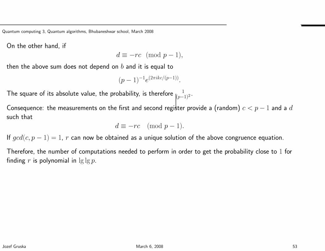
Quantum computing 3, Quantum algorithms, Bhubaneshwar school, March 2008
On the other hand, if
d ≡ −rc (mod p− 1),
then the above sum does not depend on b and it is equal to
(p− 1)−1e(2πikc/(p−1)).
The square of its absolute value, the probability, is therefore 1(p−1)2
.
Consequence: the measurements on the first and second register provide a (random) c < p− 1 and a d
such that
d ≡ −rc (mod p− 1).
If gcd(c, p − 1) = 1, r can now be obtained as a unique solution of the above congruence equation.
Therefore, the number of computations needed to perform in order to get the probability close to 1 for
finding r is polynomial in lg lg p.
Jozef Gruska March 6, 2008 53
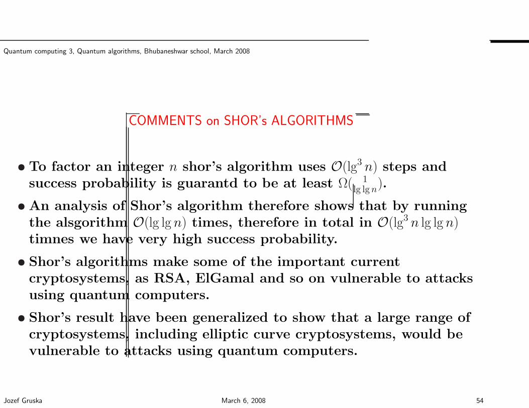
Quantum computing 3, Quantum algorithms, Bhubaneshwar school, March 2008
COMMENTS on SHOR’s ALGORITHMS
• To factor an integer n shor’s algorithm uses O(lg3 n) steps andsuccess probability is guarantd to be at least Ω( 1
lg lgn).
• An analysis of Shor’s algorithm therefore shows that by runningthe alsgorithm O(lg lg n) times, therefore in total in O(lg3 n lg lg n)timnes we have very high success probability.
• Shor’s algorithms make some of the important currentcryptosystems, as RSA, ElGamal and so on vulnerable to attacksusing quantum computers.
• Shor’s result have been generalized to show that a large range ofcryptosystems, including elliptic curve cryptosystems, would bevulnerable to attacks using quantum computers.
Jozef Gruska March 6, 2008 54
Quantum computing 3, Quantum algorithms, Bhubaneshwar school, March 2008
EXTRAS
Jozef Gruska March 6, 2008 55
Quantum computing 3, Quantum algorithms, Bhubaneshwar school, March 2008
COSETS
Given am additive group G and its subgroup G0, then a
left coset of G, with respect to G0is any set
a +G0,
where a ∈ G.
Useful fact Two cosets are either identical or disjoint.
Useful fact: Each coset has |G0| elements.
Jozef Gruska March 6, 2008 56
Quantum computing 3, Quantum algorithms, Bhubaneshwar school, March 2008
HIDDEN SUBGROUP PROBLEM
Given: An (efficiently computable) function f : G→ R, where Ggroup and R a finite set.
Promise: There exists a subgroup G0 ≤ G such that f is constantand distinct on the cossets of G0.
Task: Find a generating set for G0 (in polynomial time (in lg |G|)number of calls to the oracle for f and in the overall polynomial time).2
2A way to solve the problem is to show that in polynomial number of oracle calls (or time) the states corresponding to different candidate subgroups have exponentially smallinner product and are therefore distinguishable.
Jozef Gruska March 6, 2008 57
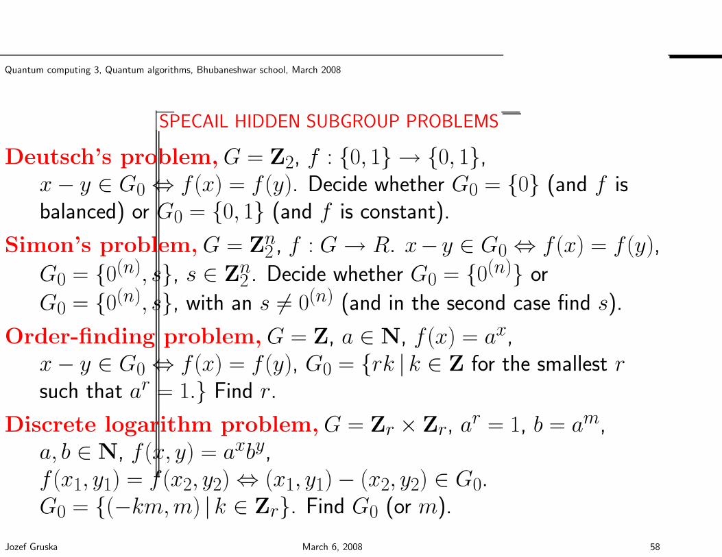
Quantum computing 3, Quantum algorithms, Bhubaneshwar school, March 2008
SPECAIL HIDDEN SUBGROUP PROBLEMS
Deutsch’s problem,G = Z2, f : 0, 1 → 0, 1,x− y ∈ G0 ⇔ f (x) = f (y). Decide whether G0 = 0 (and f isbalanced) or G0 = 0, 1 (and f is constant).
Simon’s problem,G = Zn2 , f : G→ R. x− y ∈ G0 ⇔ f (x) = f (y),
G0 = 0(n), s, s ∈ Zn2 . Decide whether G0 = 0(n) or
G0 = 0(n), s, with an s 6= 0(n) (and in the second case find s).
Order-finding problem,G = Z, a ∈ N, f (x) = ax,x− y ∈ G0 ⇔ f (x) = f (y), G0 = rk | k ∈ Z for the smallest rsuch that ar = 1. Find r.
Discrete logarithm problem,G = Zr × Zr, ar = 1, b = am,
a, b ∈ N, f (x, y) = axby,f (x1, y1) = f (x2, y2) ⇔ (x1, y1) − (x2, y2) ∈ G0.G0 = (−km,m) | k ∈ Zr. Find G0 (or m).
Jozef Gruska March 6, 2008 58
Quantum computing 3, Quantum algorithms, Bhubaneshwar school, March 2008
IMPORTANT FACTS
• Hidden subgroup problem can be solved in quantum polynomial timeif the underlying group is Abelian.
• It is an open problem whether the Hiden subgroup problem can besolved in quantum polynomial time also for any non-Abelian group.
• Would the Hideen subgroup problem be always solvable in quantumpolynomial time, this would imply that the Graph isomorphismproblem can be solved in quantum polynomial time.
Jozef Gruska March 6, 2008 59
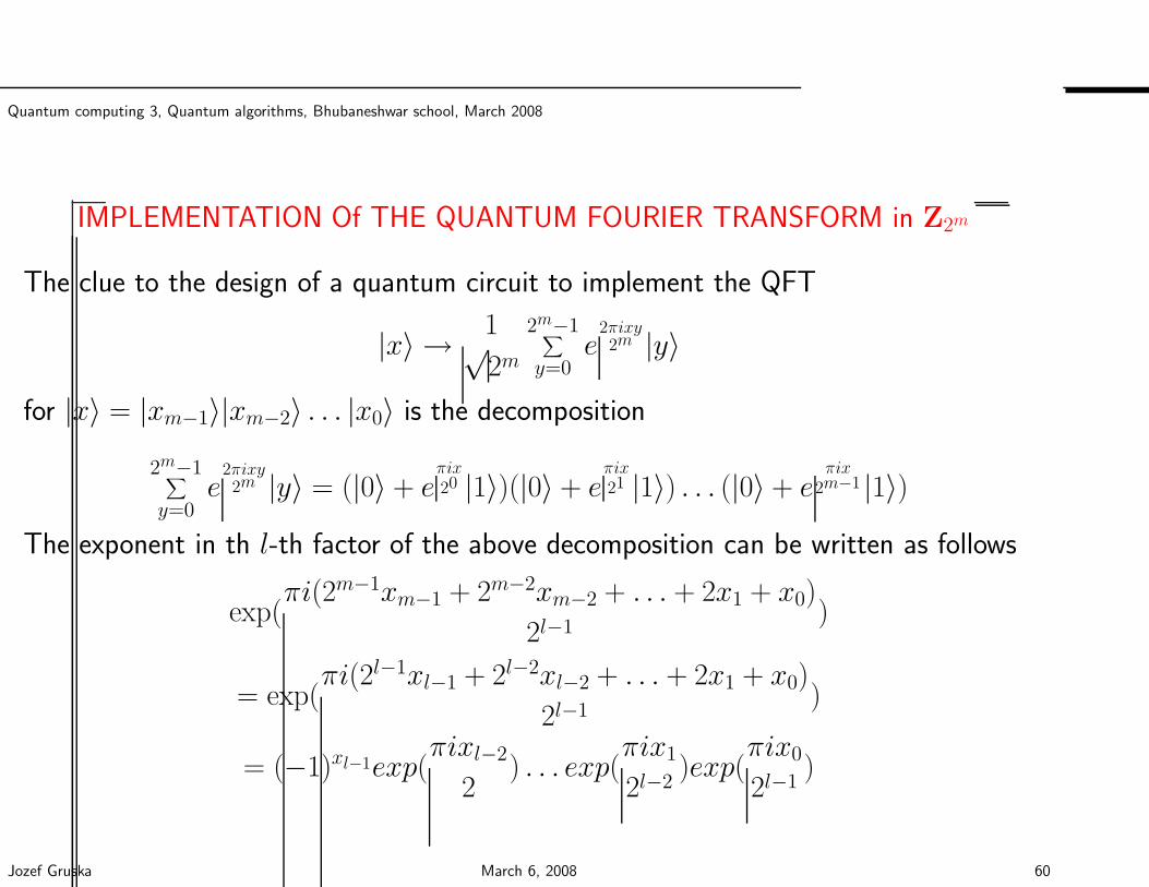
Quantum computing 3, Quantum algorithms, Bhubaneshwar school, March 2008
IMPLEMENTATION Of THE QUANTUM FOURIER TRANSFORM in Z2m
The clue to the design of a quantum circuit to implement the QFT
|x〉 → 1√2m
2m−1∑
y=0e
2πixy2m |y〉
for |x〉 = |xm−1〉|xm−2〉 . . . |x0〉 is the decomposition
2m−1∑
y=0e
2πixy2m |y〉 = (|0〉 + e
πix20 |1〉)(|0〉 + e
πix21 |1〉) . . . (|0〉 + e
πix2m−1 |1〉)
The exponent in th l-th factor of the above decomposition can be written as follows
exp(πi(2m−1xm−1 + 2m−2xm−2 + . . . + 2x1 + x0)
2l−1)
= exp(πi(2l−1xl−1 + 2l−2xl−2 + . . . + 2x1 + x0)
2l−1)
= (−1)xl−1exp(πixl−2
2) . . . exp(
πix1
2l−2)exp(
πix0
2l−1)
Jozef Gruska March 6, 2008 60
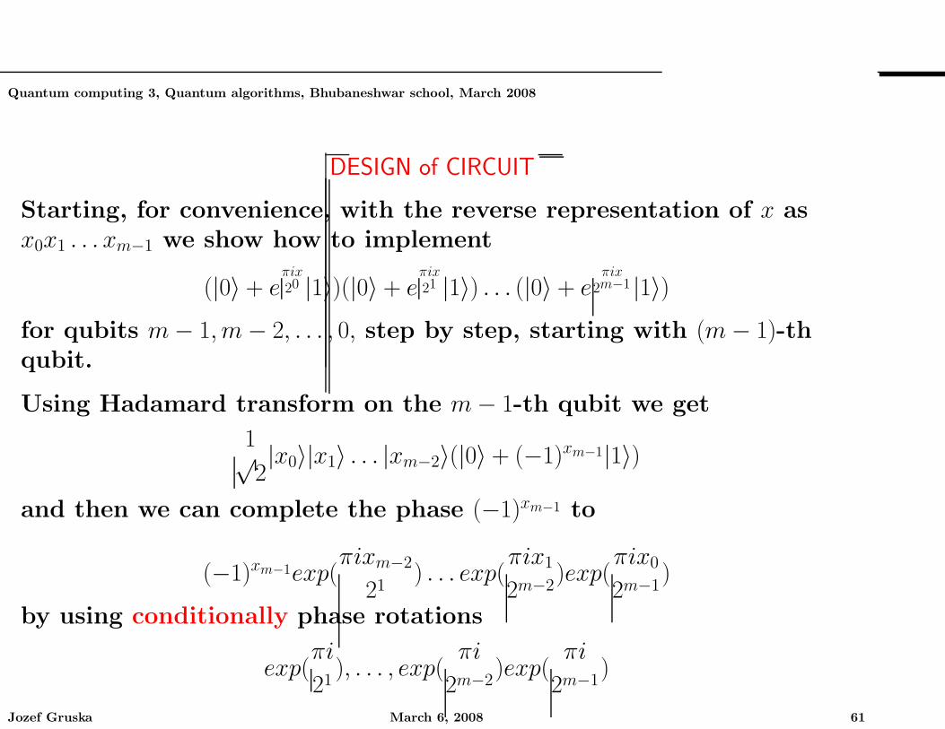
Quantum computing 3, Quantum algorithms, Bhubaneshwar school, March 2008
DESIGN of CIRCUIT
Starting, for convenience, with the reverse representation of x asx0x1 . . . xm−1 we show how to implement
(|0〉 + eπix20 |1〉)(|0〉 + e
πix21 |1〉) . . . (|0〉 + e
πix2m−1 |1〉)
for qubits m− 1,m− 2, . . . , 0, step by step, starting with (m− 1)-thqubit.
Using Hadamard transform on the m− 1-th qubit we get
1√2|x0〉|x1〉 . . . |xm−2〉(|0〉 + (−1)xm−1|1〉)
and then we can complete the phase (−1)xm−1 to
(−1)xm−1exp(πixm−2
21) . . . exp(
πix1
2m−2)exp(
πix0
2m−1)
by using conditionally phase rotations
exp(πi
21), . . . , exp(
πi
2m−2)exp(
πi
2m−1)
Jozef Gruska March 6, 2008 61
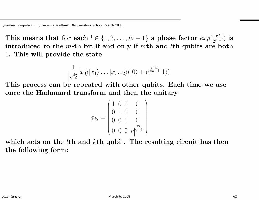
Quantum computing 3, Quantum algorithms, Bhubaneshwar school, March 2008
This means that for each l ∈ 1, 2, . . . , m− 1 a phase factor exp( πi2m−l) is
introduced to the m-th bit if and only if mth and lth qubits are both1. This will provide the state
1√2|x0〉|x1〉 . . . |xm−2〉(|0〉 + e
2πix2m−1 |1〉)
This process can be repeated with other qubits. Each time we useonce the Hadamard transform and then the unitary
φkl =
1 0 0 00 1 0 00 0 1 0
0 0 0 eπi
2l−k
which acts on the lth and kth qubit. The resulting circuit has thenthe following form:
Jozef Gruska March 6, 2008 62
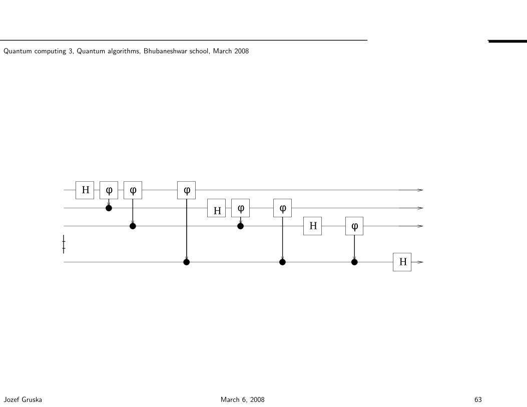
Quantum computing 3, Quantum algorithms, Bhubaneshwar school, March 2008
H
H
H
H
φ φ
φ φ
φ
φ
Jozef Gruska March 6, 2008 63
Quantum computing 3, Quantum algorithms, Bhubaneshwar school, March 2008
COMPLEXITY of FOURIER TRANSFORM
• The naive algorithm to compute all elements ofclassical Fourier transform, element by element usingbasic definition, requires O(22m) steps.
• A special recursive method, called Fast FourierTransform, that recursively reduces computation ofDFT in Z2m to computation of two DFT in Z2m−1,requires O(m2m) steps - a significant improvement.
• Quantum Fourier Transform in Z2m can be done inO(m2) quantum steps.
Jozef Gruska March 6, 2008 64
Quantum computing 3, Quantum algorithms, Bhubaneshwar school, March 2008
Moreover, in the classical case, physical representation of
(f (0), f (1), . . . , f (2m − 1))
requires Ω(2m) bits,
but in the quantum case representation of
c0|0〉 + c1|1〉 + . . . + c2m−1|2m − 1〉requires only m qubits.
Jozef Gruska March 6, 2008 65
Quantum computing 3, Quantum algorithms, Bhubaneshwar school, March 2008
FOURIER TRANSFORM on FINITE ABELIAN GROUPS
We show now basics how the concept of Fourier Transform is definedon any finite Abelian group.
Jozef Gruska March 6, 2008 66
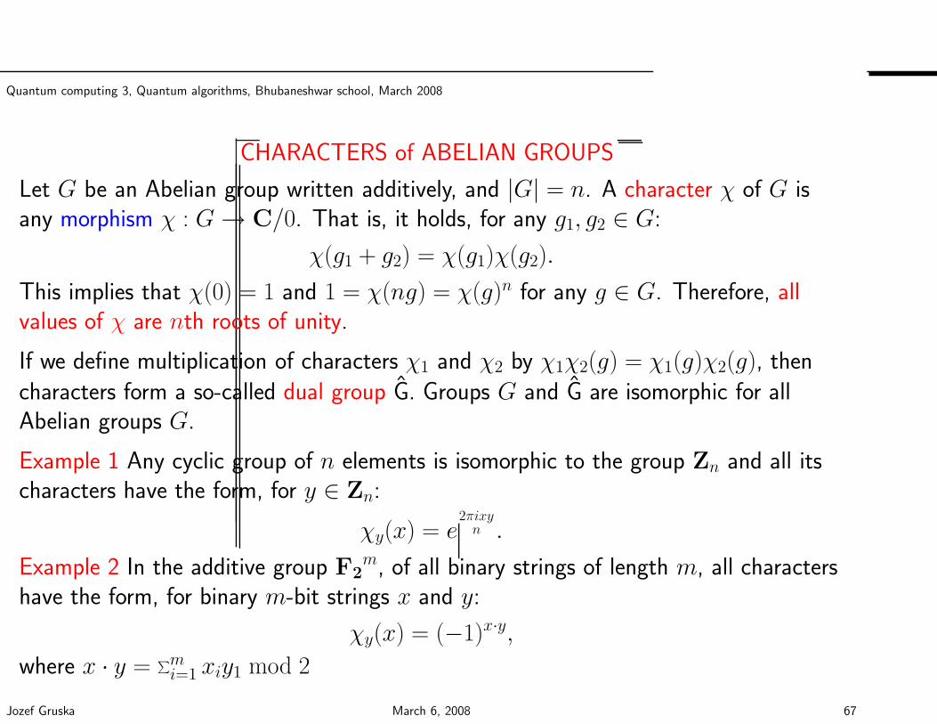
Quantum computing 3, Quantum algorithms, Bhubaneshwar school, March 2008
CHARACTERS of ABELIAN GROUPS
Let G be an Abelian group written additively, and |G| = n. A character χ of G isany morphism χ : G→ C/0. That is, it holds, for any g1, g2 ∈ G:
χ(g1 + g2) = χ(g1)χ(g2).
This implies that χ(0) = 1 and 1 = χ(ng) = χ(g)n for any g ∈ G. Therefore, allvalues of χ are nth roots of unity.
If we define multiplication of characters χ1 and χ2 by χ1χ2(g) = χ1(g)χ2(g), then
characters form a so-called dual group G. Groups G and G are isomorphic for allAbelian groups G.
Example 1 Any cyclic group of n elements is isomorphic to the group Zn and all itscharacters have the form, for y ∈ Zn:
χy(x) = e2πixyn .
Example 2 In the additive group F2m, of all binary strings of length m, all characters
have the form, for binary m-bit strings x and y:
χy(x) = (−1)x·y,
where x · y = ∑mi=1 xiy1 mod 2
Jozef Gruska March 6, 2008 67
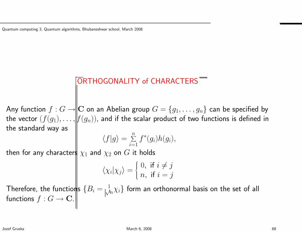
Quantum computing 3, Quantum algorithms, Bhubaneshwar school, March 2008
ORTHOGONALITY of CHARACTERS
Any function f : G→ C on an Abelian group G = g1, . . . , gn can be specified bythe vector (f(g1), . . . , f(gn)), and if the scalar product of two functions is defined inthe standard way as
〈f |g〉 =n∑
i=1f∗(gi)h(gi),
then for any characters χ1 and χ2 on G it holds
〈χi|χj〉 =
0, if i 6= jn, if i = j
Therefore, the functions Bi = 1√nχi form an orthonormal basis on the set of all
functions f : G→ C.
Jozef Gruska March 6, 2008 68
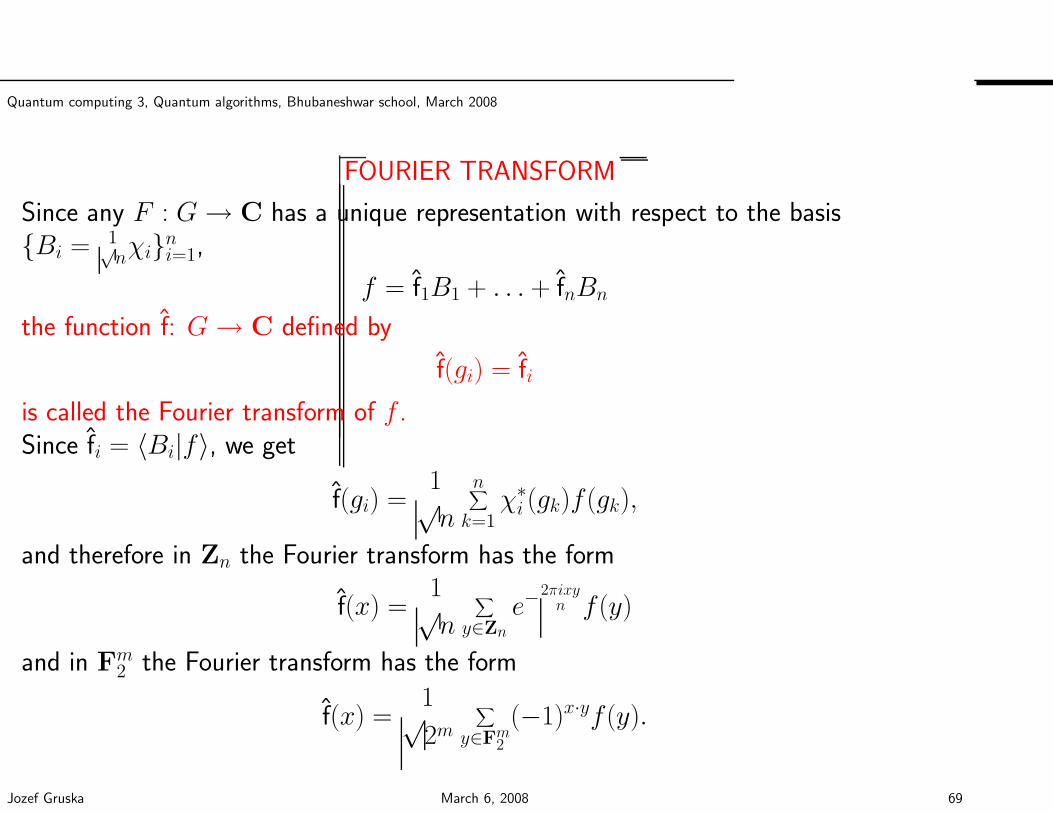
Quantum computing 3, Quantum algorithms, Bhubaneshwar school, March 2008
FOURIER TRANSFORM
Since any F : G→ C has a unique representation with respect to the basisBi = 1√
nχini=1,
f = f1B1 + . . . + fnBn
the function f: G→ C defined by
f(gi) = fi
is called the Fourier transform of f .Since fi = 〈Bi|f〉, we get
f(gi) =1√n
n∑
k=1χ∗i (gk)f(gk),
and therefore in Zn the Fourier transform has the form
f(x) =1√n
∑
y∈Zne−
2πixyn f(y)
and in Fm2 the Fourier transform has the form
f(x) =1√2m
∑
y∈Fm2
(−1)x·yf(y).
Jozef Gruska March 6, 2008 69
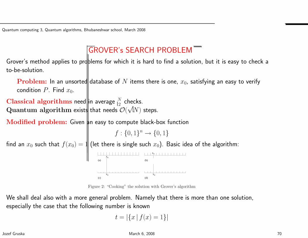
Quantum computing 3, Quantum algorithms, Bhubaneshwar school, March 2008
GROVER’s SEARCH PROBLEM
Grover’s method applies to problems for which it is hard to find a solution, but it is easy to check a
to-be-solution.
Problem: In an unsorted database of N items there is one, x0, satisfying an easy to verify
condition P . Find x0.
Classical algorithms need in average N2 checks.
Quantum algorithm exists that needs O(√N) steps.
Modified problem: Given an easy to compute black-box function
f : 0, 1n → 0, 1find an x0 such that f(x0) = 1 (let there is single such x0). Basic idea of the algorithm:
(a)x
x x
(b)
(c) (d)
0
0 0
x0
Figure 2: “Cooking” the solution with Grover’s algorithm
We shall deal also with a more general problem. Namely that there is more than one solution,
especially the case that the following number is known
t = |x | f(x) = 1|
Jozef Gruska March 6, 2008 70
Quantum computing 3, Quantum algorithms, Bhubaneshwar school, March 2008
INVERSION ABOUT THE AVERAGE
Example 0.4 (Inversion about the average) The unitary transformation
Dn :2n−1∑
i=0ai|φi〉 →
2n−1∑
i=0(2E − ai)|φi〉,
where E is the average of ai | 0 ≤ i < 2n, can be performed by the matrix
−HnVn0 Hn = Dn =
−1 + 22n
22n . . . 2
2n
22n −1 + 2
2n. . . 2
2n
... ... . . . ...22n
22n . . . −1 + 2
2n
.
The name of the operation comes from the fact that 2E − x = E +E − x and therefore the new value is
as much above (below) the average as it was initially below (above) the average—which is precisely the
inversion about the average.
The matrix Dn is clearly unitary and it can be shown to have the form Dn = −HnVn0 Hn, where
V n0 [i, j] = 0 if i 6= j, V n
0 [1, 1] = −1 and V n0 [i, i] = 1 if 1 < i ≤ n.
Jozef Gruska March 6, 2008 71
Quantum computing 3, Quantum algorithms, Bhubaneshwar school, March 2008
Let us consider again the unitary transformation
Dn :2n−1∑
i=0ai|φi〉 →
2n−1∑
i=0(2E − ai)|φi〉,
and the following example:
Example: Let ai = a if i 6= x0 and ax0= −a. Then
E = a− 2
2na
2E − ai =
a− 42na if i 6= x0
2E − ax0= 3a− 4
2na; otherwise
Jozef Gruska March 6, 2008 72
Quantum computing 3, Quantum algorithms, Bhubaneshwar school, March 2008
GROVER’s SEARCH ALGORITHM
Start in the state
|φ〉 =1√2n
2n−1∑
x=0|x〉
and iterate ⌊π4√
2n⌋ times the transformation
−HnVn0 HnVf
︸ ︷︷ ︸
|φ〉 → |φ〉.Grover’s iterate
Finally, measure the register to get x0 and check whether f(x0) = 1. If not, repeat the procedure.
It has been shown that the above algorithm is optimal for finding the solution with probability > 12.
In the case that there are t solutions, repeat the above iteration
π
4
√√√√√
2n
t
times
Jozef Gruska March 6, 2008 73
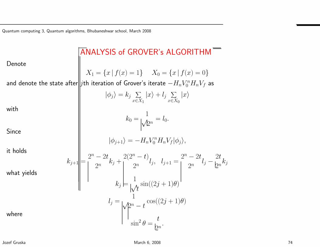
Quantum computing 3, Quantum algorithms, Bhubaneshwar school, March 2008
ANALYSIS of GROVER’s ALGORITHM
Denote
X1 = x | f(x) = 1 X0 = x | f(x) = 0and denote the state after jth iteration of Grover’s iterate −HnV
n0 HnVf as
|φj〉 = kj∑
x∈X1
|x〉 + lj∑
x∈X0
|x〉
with
k0 =1√2n
= l0.
Since
|φj+1〉 = −HnVn0 HnVf |φj〉,
it holds
kj+1 =2n − 2t
2nkj +
2(2n − t)
2nlj, lj+1 =
2n − 2t
2nlj −
2t
2nkj
what yields
kj =1√tsin((2j + 1)θ)
lj =1√
2n − tcos((2j + 1)θ)
where
sin2 θ =t
2n.
Jozef Gruska March 6, 2008 74
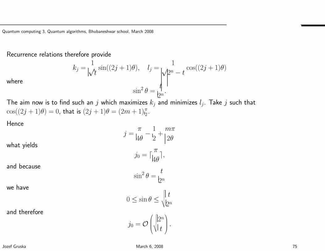
Quantum computing 3, Quantum algorithms, Bhubaneshwar school, March 2008
Recurrence relations therefore provide
kj =1√tsin((2j + 1)θ), lj =
1√2n − t
cos((2j + 1)θ)
where
sin2 θ =t
2n.
The aim now is to find such an j which maximizes kj and minimizes lj. Take j such that
cos((2j + 1)θ) = 0, that is (2j + 1)θ = (2m + 1)π2 .
Hence
j =π
4θ− 1
2+mπ
2θwhat yields
j0 = ⌈ π4θ
⌉,and because
sin2 θ =t
2nwe have
0 ≤ sin θ ≤√√√√√t
2n
and therefore
j0 = O
√√√√√
2n
t
.
Jozef Gruska March 6, 2008 75
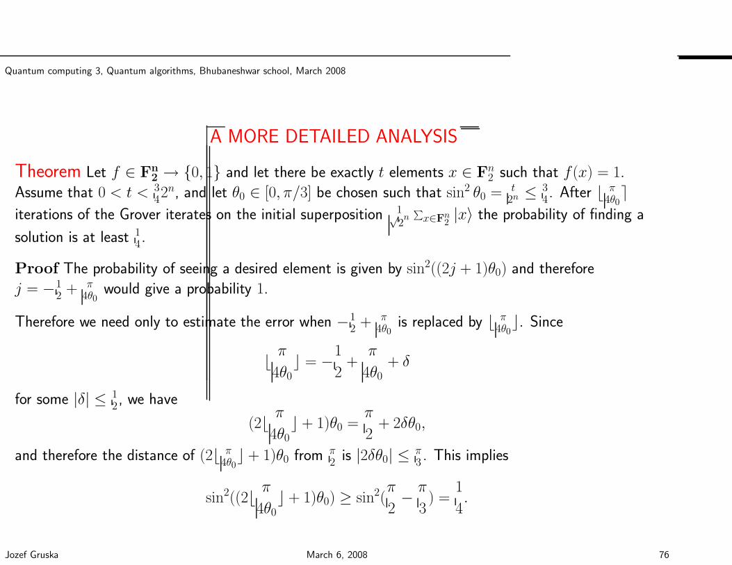
Quantum computing 3, Quantum algorithms, Bhubaneshwar school, March 2008
A MORE DETAILED ANALYSIS
Theorem Let f ∈ Fn2 → 0, 1 and let there be exactly t elements x ∈ Fn
2 such that f(x) = 1.
Assume that 0 < t < 342n, and let θ0 ∈ [0, π/3] be chosen such that sin2 θ0 = t
2n ≤ 34. After ⌊ π
4θ0⌉
iterations of the Grover iterates on the initial superposition 1√2n
∑
x∈Fn2|x〉 the probability of finding a
solution is at least 14.
Proof The probability of seeing a desired element is given by sin2((2j + 1)θ0) and therefore
j = −12
+ π4θ0
would give a probability 1.
Therefore we need only to estimate the error when −12 + π
4θ0is replaced by ⌊ π
4θ0⌋. Since
⌊ π4θ0
⌋ = −1
2+
π
4θ0+ δ
for some |δ| ≤ 12, we have
(2⌊ π4θ0
⌋ + 1)θ0 =π
2+ 2δθ0,
and therefore the distance of (2⌊ π4θ0
⌋ + 1)θ0 from π2
is |2δθ0| ≤ π3. This implies
sin2((2⌊ π4θ0
⌋ + 1)θ0) ≥ sin2(π
2− π
3) =
1
4.
Jozef Gruska March 6, 2008 76
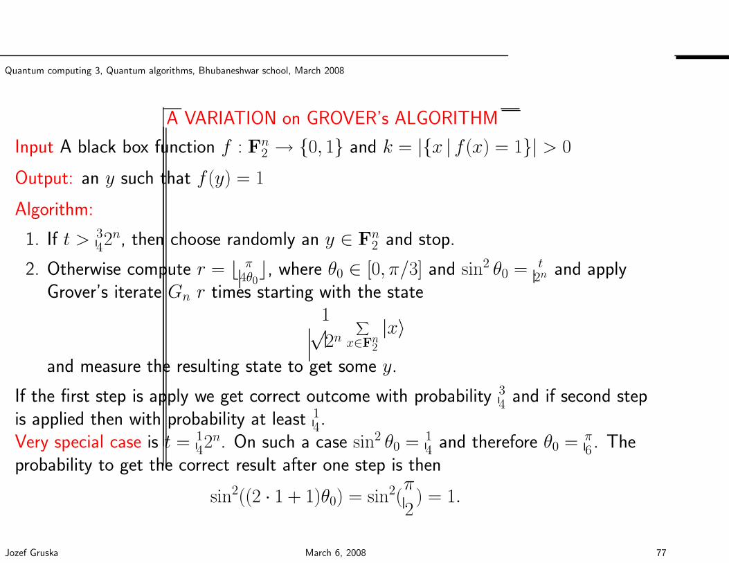
Quantum computing 3, Quantum algorithms, Bhubaneshwar school, March 2008
A VARIATION on GROVER’s ALGORITHM
Input A black box function f : Fn2 → 0, 1 and k = |x | f(x) = 1| > 0
Output: an y such that f(y) = 1
Algorithm:
1. If t > 342n, then choose randomly an y ∈ Fn
2 and stop.
2. Otherwise compute r = ⌊ π4θ0
⌋, where θ0 ∈ [0, π/3] and sin2 θ0 = t2n and apply
Grover’s iterate Gn r times starting with the state1√2n
∑
x∈Fn2
|x〉
and measure the resulting state to get some y.
If the first step is apply we get correct outcome with probability 34 and if second step
is applied then with probability at least 14.
Very special case is t = 142n. On such a case sin2 θ0 = 1
4and therefore θ0 = π
6. The
probability to get the correct result after one step is then
sin2((2 · 1 + 1)θ0) = sin2(π
2) = 1.
Jozef Gruska March 6, 2008 77
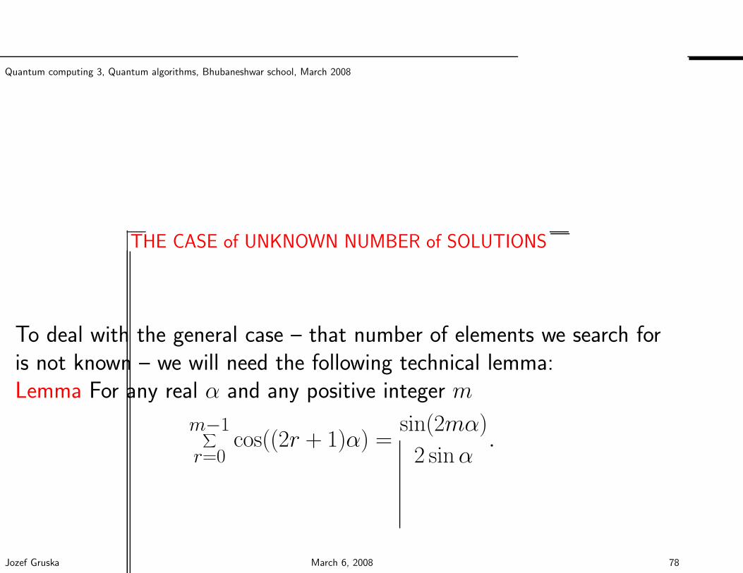
Quantum computing 3, Quantum algorithms, Bhubaneshwar school, March 2008
THE CASE of UNKNOWN NUMBER of SOLUTIONS
To deal with the general case – that number of elements we search foris not known – we will need the following technical lemma:Lemma For any real α and any positive integer m
m−1∑
r=0cos((2r + 1)α) =
sin(2mα)
2 sinα.
Jozef Gruska March 6, 2008 78
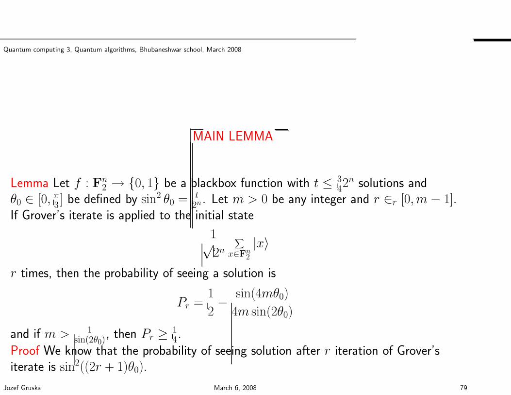
Quantum computing 3, Quantum algorithms, Bhubaneshwar school, March 2008
MAIN LEMMA
Lemma Let f : Fn2 → 0, 1 be a blackbox function with t ≤ 3
42n solutions and
θ0 ∈ [0, π3] be defined by sin2 θ0 = t
2n. Let m > 0 be any integer and r ∈r [0,m− 1].
If Grover’s iterate is applied to the initial state
1√2n
∑
x∈Fn2
|x〉
r times, then the probability of seeing a solution is
Pr =1
2− sin(4mθ0)
4m sin(2θ0)
and if m > 1sin(2θ0)
, then Pr ≥ 14.
Proof We know that the probability of seeing solution after r iteration of Grover’siterate is sin2((2r + 1)θ0).
Jozef Gruska March 6, 2008 79
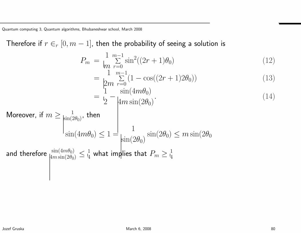
Quantum computing 3, Quantum algorithms, Bhubaneshwar school, March 2008
Therefore if r ∈r [0,m− 1], then the probability of seeing a solution is
Pm =1
m
m−1∑
r=0sin2((2r + 1)θ0) (12)
=1
2m
m−1∑
r=0(1 − cos((2r + 1)2θ0)) (13)
=1
2− sin(4mθ0)
4m sin(2θ0). (14)
Moreover, if m ≥ 1sin(2θ0)
, then
sin(4mθ0) ≤ 1 =1
sin(2θ0)sin(2θ0) ≤ m sin(2θ0
and therefore sin(4mθ0)4m sin(2θ0)
≤ 14 what implies that Pm ≥ 1
4
Jozef Gruska March 6, 2008 80
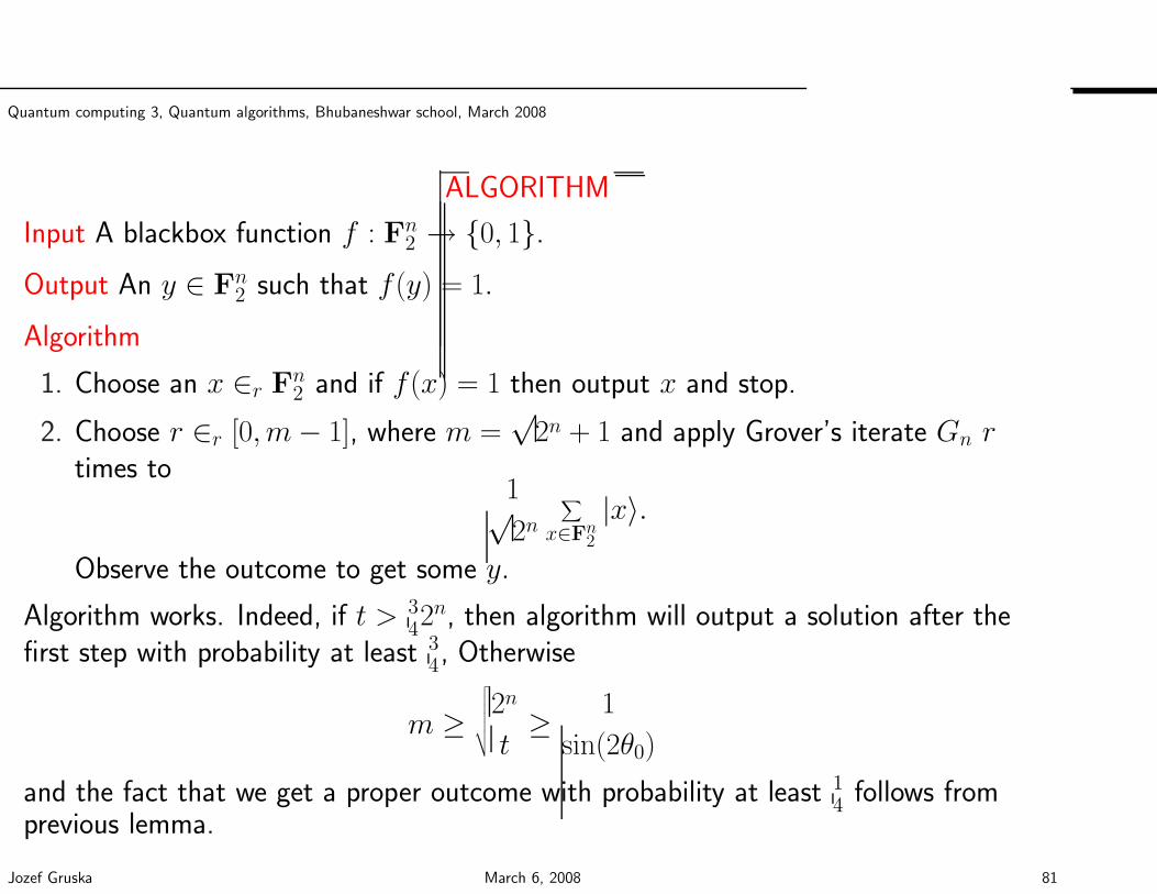
Quantum computing 3, Quantum algorithms, Bhubaneshwar school, March 2008
ALGORITHM
Input A blackbox function f : Fn2 → 0, 1.
Output An y ∈ Fn2 such that f(y) = 1.
Algorithm
1. Choose an x ∈r Fn2 and if f(x) = 1 then output x and stop.
2. Choose r ∈r [0,m− 1], where m =√
2n + 1 and apply Grover’s iterate Gn rtimes to
1√2n
∑
x∈Fn2
|x〉.
Observe the outcome to get some y.
Algorithm works. Indeed, if t > 342n, then algorithm will output a solution after the
first step with probability at least 34, Otherwise
m ≥√√√√√√
2n
t≥ 1
sin(2θ0)
and the fact that we get a proper outcome with probability at least 14
follows fromprevious lemma.
Jozef Gruska March 6, 2008 81
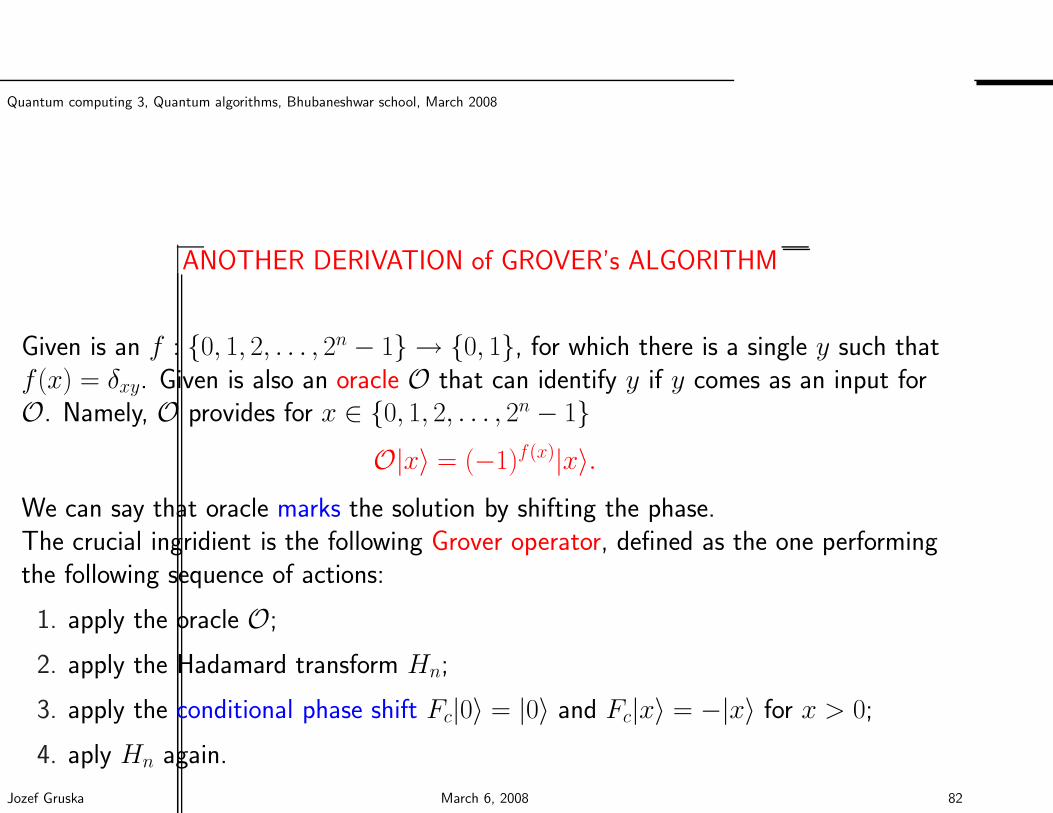
Quantum computing 3, Quantum algorithms, Bhubaneshwar school, March 2008
ANOTHER DERIVATION of GROVER’s ALGORITHM
Given is an f : 0, 1, 2, . . . , 2n − 1 → 0, 1, for which there is a single y such thatf(x) = δxy. Given is also an oracle O that can identify y if y comes as an input forO. Namely, O provides for x ∈ 0, 1, 2, . . . , 2n − 1
O|x〉 = (−1)f(x)|x〉.We can say that oracle marks the solution by shifting the phase.The crucial ingridient is the following Grover operator, defined as the one performingthe following sequence of actions:
1. apply the oracle O;
2. apply the Hadamard transform Hn;
3. apply the conditional phase shift Fc|0〉 = |0〉 and Fc|x〉 = −|x〉 for x > 0;
4. aply Hn again.
Jozef Gruska March 6, 2008 82
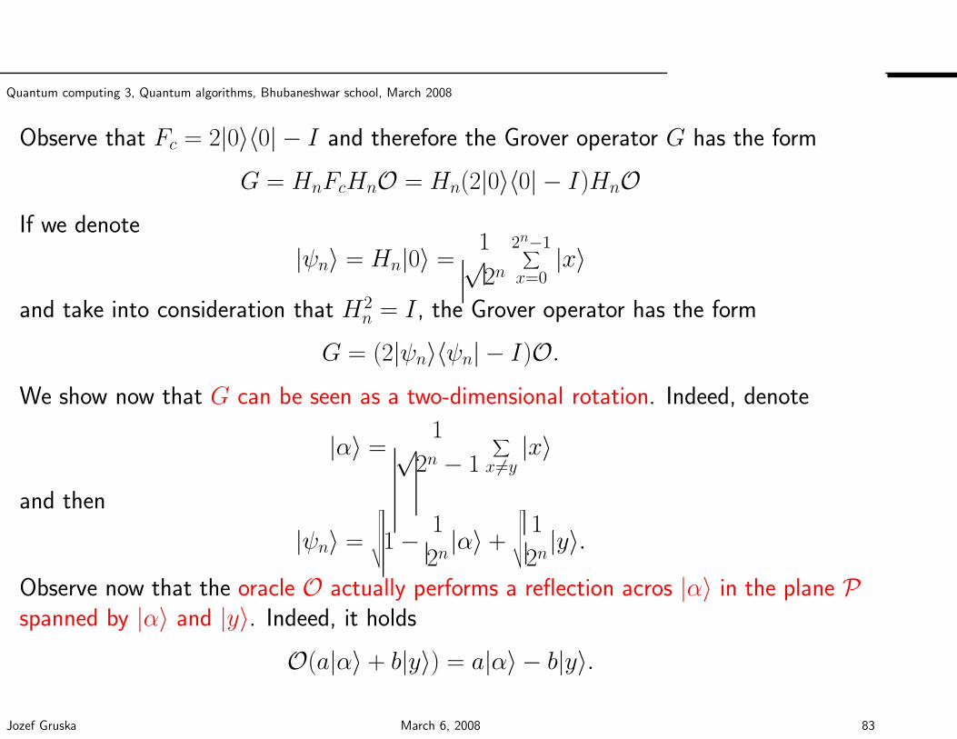
Quantum computing 3, Quantum algorithms, Bhubaneshwar school, March 2008
Observe that Fc = 2|0〉〈0| − I and therefore the Grover operator G has the form
G = HnFcHnO = Hn(2|0〉〈0| − I)HnOIf we denote
|ψn〉 = Hn|0〉 =1√2n
2n−1∑
x=0|x〉
and take into consideration that H2n = I , the Grover operator has the form
G = (2|ψn〉〈ψn| − I)O.We show now that G can be seen as a two-dimensional rotation. Indeed, denote
|α〉 =1√
2n − 1
∑
x 6=y|x〉
and then
|ψn〉 =
√√√√√√1 − 1
2n|α〉 +
√√√√√√
1
2n|y〉.
Observe now that the oracle O actually performs a reflection acros |α〉 in the plane Pspanned by |α〉 and |y〉. Indeed, it holds
O(a|α〉 + b|y〉) = a|α〉 − b|y〉.
Jozef Gruska March 6, 2008 83
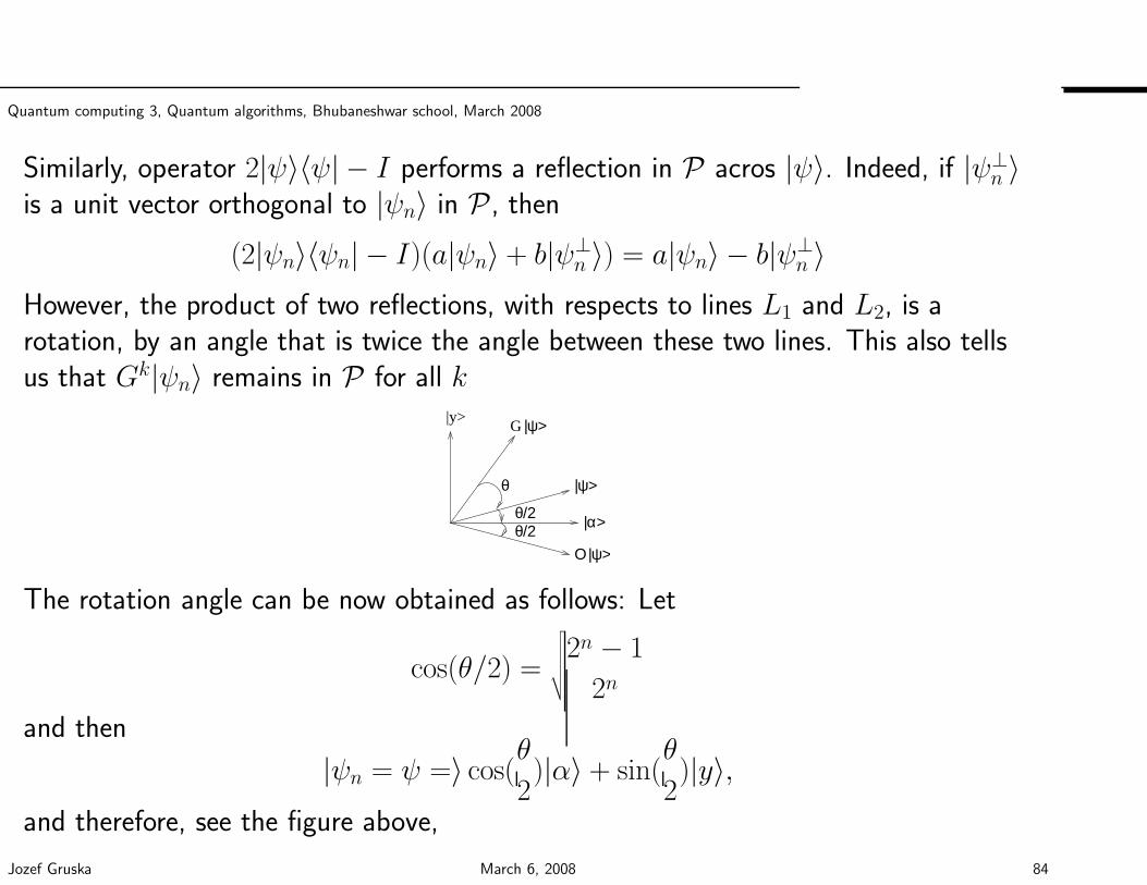
Quantum computing 3, Quantum algorithms, Bhubaneshwar school, March 2008
Similarly, operator 2|ψ〉〈ψ| − I performs a reflection in P acros |ψ〉. Indeed, if |ψ⊥n 〉
is a unit vector orthogonal to |ψn〉 in P , then
(2|ψn〉〈ψn| − I)(a|ψn〉 + b|ψ⊥n 〉) = a|ψn〉 − b|ψ⊥
n 〉However, the product of two reflections, with respects to lines L1 and L2, is arotation, by an angle that is twice the angle between these two lines. This also tellsus that Gk|ψn〉 remains in P for all k
|y>G |ψ>
θ
θ/2θ/2
|ψ>
|α>
O |ψ>
The rotation angle can be now obtained as follows: Let
cos(θ/2) =
√√√√√√
2n − 1
2n
and then
|ψn = ψ =〉 cos(θ
2)|α〉 + sin(
θ
2)|y〉,
and therefore, see the figure above,
Jozef Gruska March 6, 2008 84
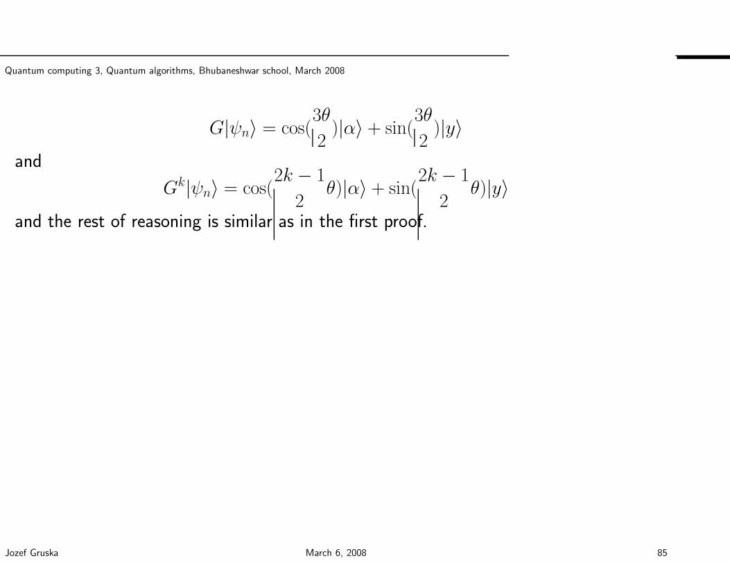
Quantum computing 3, Quantum algorithms, Bhubaneshwar school, March 2008
G|ψn〉 = cos(3θ
2)|α〉 + sin(
3θ
2)|y〉
and
Gk|ψn〉 = cos(2k − 1
2θ)|α〉 + sin(
2k − 1
2θ)|y〉
and the rest of reasoning is similar as in the first proof.
Jozef Gruska March 6, 2008 85
Quantum computing 3, Quantum algorithms, Bhubaneshwar school, March 2008
QUANTUM SEARCH in ORDERED LISTS
A related problem to that of a search in an unordered list is a search inan ordered list of n items.
• The best upper bound known today is 34 lgn.
• The best lower bound known today is 112 lg n−O(1).
Jozef Gruska March 6, 2008 86
Quantum computing 3, Quantum algorithms, Bhubaneshwar school, March 2008
EFFICIENCY of GROVER’s SEARCH
There are at least four different proofs that Grover’s search isasymptotically optimal.
Quite a bit is known about the relation between the error ε and thenumber T of queries when searching an unordered list of n elements.
• ε can be an arbitrary small constant if O(√n) queries are used, but
not when o(√n) queries are used.
• ε can be at most 12nα using O(n0.5+α) queries.
• To achieve no error (ε = 0), θ(n) queries are needed.
Jozef Gruska March 6, 2008 87
Quantum computing 3, Quantum algorithms, Bhubaneshwar school, March 2008
APPLICATIONS of GROVER’s SEARCH
There is a variety of applications of Grover’s search algorithm. Let us mention some of them.
• Extremes of functions computation (minimum, maximum).
• Collision problem Task is to find, for a given black-box function f : X → Y , two different
x 6= y such that f(x) = f(y), given a promise that such a pair exist.
On a more general level an analogical problem deals with the so-called r-to-one functions every
element of their image has exactly r pre-images. It has been shown that there is a quantum
algorithm to solve collision problem for r-to-one functions in quantum time O((n/r)1/3). It has been
shown in 2003 by Shi that the above upper bound cannot be asymptotically improved.
• Verification of predicate calculus formulas. Grover’s search algorithm can be seen as a
method to verify formulas
∃xP (x),
where P is a black-box predicate.
It has been shown that also more generalized formulas of the type
∀x1∃y1∀x2∃y2 . . . ∀xk∃ykP (x1, y1, x2, y2, . . . , xk, yk)
can be verified quantumly with the number of queries O(√
2(2k)).
Jozef Gruska March 6, 2008 88
Quantum computing 3, Quantum algorithms, Bhubaneshwar school, March 2008
QUANTUM MINIMUM FINDING ALGORITHM
Problem: Let s = s1, s2, . . . , sn be an unsorted sequence of distinct elements. Find an m such that
sm is minimal.
Classical search algorithm needs θ(n) comparisons.
QUANTUM SEARCH ALGORITHM
1. Choose as a first “threshold” a random y ∈ 1, . . . , n.2. Repeat the following three steps until the total running time is more than 22.5
√n + 1.4 lg2 n.
2.1. Initialize
|ψ0〉 =1√n
n∑
i=1|i〉|y〉
and consider an index i as marked if si < sy.
2.2. Apply Grover search to the first register to find an marked element.
2.3. Measure the first register. If y′ is the outcome and sy′ < sy, take as a new threshold the index
y′.
3. Return as the output the last threshold y.
It is shown in my book that the above algorithm finds the minimum with probability at least 12
if the
measurement is done after a total number of θ(√n) operations.
Jozef Gruska March 6, 2008 89