Introduction to probability BSAD 30 Dave Novak Source: Anderson et al., 2013 Quantitative Methods for Business 12 th edition – some slides are directly

Introduction to probability

BSAD 30

Dave Novak

Source: Anderson et al., 2013 Quantitative Methods for Business 12th edition – some slides are directly from J. Loucks © 2013 Cengage Learning

Overview

Experiments and the Sample Space Assigning Probabilities to Experimental

Outcomes Events and Their Probabilities Some Basic Relationships of Probability Bayes’ Theorem Simpson’s Paradox

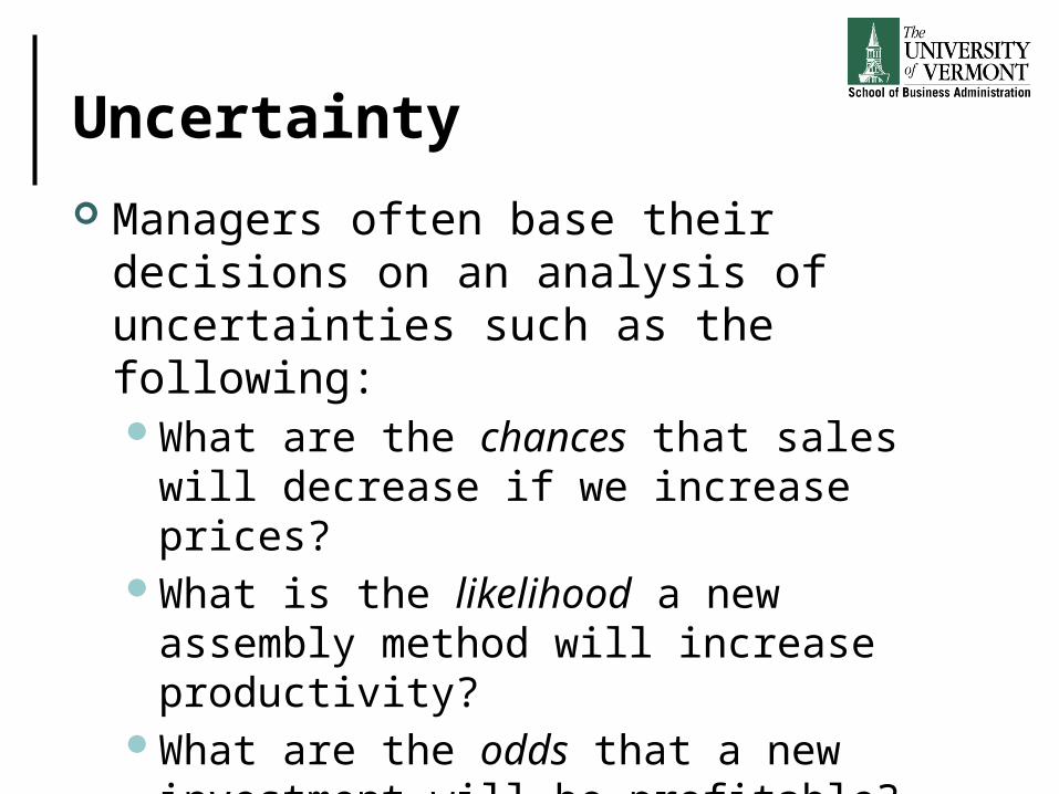
Uncertainty

Managers often base their decisions on an analysis of uncertainties such as the following:What are the chances that sales will

decrease if we increase prices?What is the likelihood a new assembly

method will increase productivity?What are the odds that a new investment will

be profitable?

Probability

Probability is a numerical measure of the likelihood that an event will occur

Probability values are always assigned on a scale from 0 to 1 You can think of probability in terms of

percentage A probability near zero indicates an event is

quite unlikely to occur A probability near one indicates an event is

almost certain to occur

Probability as a numerical measure of likelihood

0 1.5

Increasing Likelihood of Occurrence

Probability:

The eventis veryunlikelyto occur

The occurrenceof the event is just as likely asit is unlikely

The eventis almostcertainto occur

Statistical experiments

A statistical experiment differs somewhat from an experiment in the physical sciences

In statistical experiments, probability determines outcomes

Even though the experiment is repeated in exactly the same way, an entirely different outcome may occur

For this reason, statistical experiments are often called random experiments

An experiment and its sample space An experiment is any process that

generates well-defined outcomes Flipping a coin 10 times

The sample space for an experiment is the set of all experimental outcomes The exact H or T results from all 10 times

An experimental outcome is also called a sample pointThe result of a particular coin flip

An experiment and its sample space

ExperimentToss a coinInspection a partConduct a sales callRoll a diePlay a football game

Sample SpaceHead, tailDefective, non-defectivePurchase, no purchase1, 2, 3, 4, 5, 6Win, lose, tie

Assigning probabilities

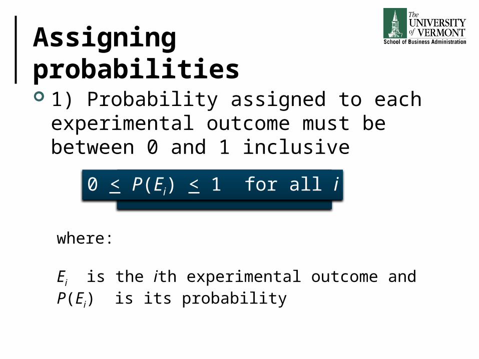
1) Probability assigned to each experimental outcome must be between 0 and 1 inclusive

0 < P(Ei) < 1 for all i

where:

Ei is the ith experimental outcome and P(Ei) is its probability


2) The sum of the probabilities for all experimental outcomes must be equal to 1

P(E1) + P(E2) + . . . + P(En) = 1

where:n is the number of experimental outcomes

Assigning probabilities If we throw two dice together, the possible

outcomes are: 2, 3, 4, … 12 However, each outcome is not equally likely What is the probability that each outcome

will occur?


Total of Dice Specific Outcomes on Pairs of Dice Probability Event Occurs

2 D1=1 + D2=1 (1+1) 1/36 = 3%

3 D1=1 + D2=2 (1+2), D1=2 + D2=1 (2+1) 2/36 = 1/18 = 6%

4 1+3, 2+2, 3+1 3/36 = 1/12 = 8%

5 1+4, 2+3, 3+2, 4+1 4/36 = 1/9 = 11%

6 1+5, 2+4, 3+3, 4+2, 5+1 5/36 = 14%

7 1+6, 2+5, 3+4, 4+3, 5+2, 6+1 6/36 = 1/6 = 17%

8 2+6, 3+5, 4+4, 5+3, 6+2 5/36 = 14%

9 3+6, 4+5, 5+4, 6+3 4/36 = 1/9 = 11%

10 4+6, 5+5, 6+4 3/36 = 1/12 = 8%

11 5+6, 6+5 2/36 = 1/18 = 6%

12 6+6 1/36 = 3%


P(E1) + P(E2) + . . . + P(En) = 1

Assigning probabilities Three ways of assigning probabilities

1) Classical method• Assume equally likely outcomes

2) Relative frequency method• Assign probabilities based on experimentation or

historical data

3) Subjective method• Assign probabilities based on judgment

Classical method Rolling a die

If an experiment has n possible outcomes (where n=6), the classical method would assign a probability of 1/n to each outcome

Sample Space: S = {1, 2, 3, 4, 5, 6}

Probabilities: Each sample point has a 1/6 (or 0.166) chance of occurring

Relative frequency method

Lucas Tool Rental would like to assign probabilities to the number of car polishers it rents each day. Office records show the following frequencies of daily rentals for the last 40 days

Number ofPolishers Rented

Numberof Days

01234

4 61810 2

Relative frequency methodEach probability assignment is given by dividingthe frequency (number of days) by the total frequency(total number of days)

4/40Probability

Number ofPolishers Rented

Numberof Days

01234

4 61810 240

.10 .15 .45 .25 .051.00

10/40

Subjective method When economic conditions and a

company’s circumstances change rapidly it might be inappropriate to assign probabilities based solely on historical data

We can use any data available as well as our experience and intuition, but ultimately a probability value should express our degree of belief that the experimental outcome will occurWhat is a potentially serious drawback

associated with this approach?

Subjective method Consider the case in which a couple just

made an offer to purchase a house. Two outcomes are possible:

One believes the probability their offer will be accepted is 0.8; thus, P(E1) = 0.8 and P(E2) = 0.2. Two, believes the

probability that their offer will be accepted is 0.6; hence, P(E1) = 0.6 and P(E2) = 0.4. Person two’s probability

estimate for E1 reflects a greater pessimism that their

offer will be accepted

E1 = their offer is accepted

E2 = their offer is rejected

Events and their probabilities An event is a collection of sample points The probability of any event is equal to the

sum of the probabilities of the sample points in the event

If we can identify all the sample points of an experiment and assign a probability to each sample point, we can compute the probability of the event

Events and their probabilities Rolling a die

Event E = Probability of getting an even number when rolling a die

E = {2, 4, 6}

P(E) = P(2) + P(4) + P(6)

= 1/6 + 1/6 + 1/6

= 3/6 = .5

Four relationships of probability These relationships can be used to compute

the probability of an event, without knowing all the sample point probabilities1) Compliment of an event2) Addition law3) Conditional probabilities4) Multiplication law

Example

You invest in two stocks: Markley Oil and Collins Mining, and determine that the possible outcomes of these investments three months from now are:

Investment Gain or Loss in 3 Months (in $000)

Markley Oil Collins Mining

10 5 0-20

8-2

Example Assume an analyst makes the following

probability estimates

Exper. Outcome Net Gain or Loss Probability

(10, 8)(10, -2)(5, 8)(5, -2)(0, 8)(0, -2)(-20, 8)(-20, -2)

$18,000 Gain $8,000 Gain $13,000 Gain $3,000 Gain $8,000 Gain $2,000 Loss $12,000 Loss $22,000 Loss

.20

.08

.16

.26

.10

.12

.02

.06

Example Viewed as a tree diagram

Gain 5Gain 5

Gain 8Gain 8

Gain 8Gain 8

Gain 10Gain 10

Gain 8Gain 8

Gain 8Gain 8

Lose 20Lose 20

Lose 2Lose 2

Lose 2Lose 2

Lose 2Lose 2

Lose 2Lose 2

EvenEven

Markley Oil(Stage 1)

Collins Mining(Stage 2)

ExperimentalOutcomes

(10, 8) Gain $18,000

(10, -2) Gain $8,000

(5, 8) Gain $13,000

(5, -2) Gain $3,000

(0, 8) Gain $8,000

(0, -2) Lose $2,000

(-20, 8) Lose $12,000

(-20, -2) Lose $22,000

Example Compute the probability that your

investment in Markley Oil will be profitable

Example Compute the probability that your

investment in Collins Mining will be profitable

Complement of an event The complement of event A is defined to be

the event consisting of all sample points that are not in A

Event A Ac

SampleSpace SSampleSpace S

VennDiagram

Union of two events The union of events A and B is the event

containing all sample points that are in A or B or both

The union of events A and B is denoted by A B

SampleSpace SSampleSpace SEvent A Event B

Example Compute the probability of the union of two

events

Example Compute the probability of the union of two

events

Intersection of two events The intersection of events A and B is the set

of all sample points that are in both A and B

The intersection of events A and B is denoted by A


Intersection of A and BIntersection of A and B

Example Compute the probability of the intersection

of two events

Addition law The addition law provides a way to compute

the probability of event A, or B, or both A and B occurring

The addition law is written as:

P(A B) = P(A) + P(B) - P(A B

Example Demonstrate the addition law

Mutually exclusive events Two events are said to be mutually

exclusive if the events have no sample points in common

Two events are mutually exclusive if, when one event occurs, the other cannot occur


Mutually exclusive events If events A and B are mutually exclusive,

P(A B = 0 In this case, the addition law is:

P(A B) = P(A) + P(B)

There is no need toinclude “- P(A B”

Conditional probability The probability of an event occurring given

that another event has already occurred is called a conditional probability

A conditional probability is computed as:

The conditional probability of A given B is denoted by P(A|B)

( )( | )

( )P A B

P A BP B

Example Calculate a conditional probability



Multiplication law The multiplication law provides a way to

compute the probability of the intersection of two events

The multiplication law is written as:

P(A B) = P(B) P(A|B)

Example Demonstrate the multiplication law

Joint and marginal conditional probabilities A joint probability gives the probability of an

intersection of two events A marginal probability gives the probability

of each single event separately These probabilities are often shown in a

joint probability table

Joint and marginal conditional probabilities

Collins MiningProfitable (C) Not Profitable (Cc)Markley Oil

Profitable (M) Not Profitable (Mc)

Total .48 .52

Total

.70

.30

1.00

.36 .34

.12 .18

Joint Probabilities(appear in the bodyof the table)

Marginal Probabilities(appear in the marginsof the table)

Example Where are the values in the table coming

from?

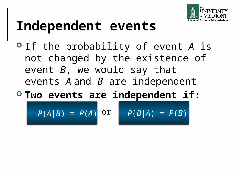
Independent events If the probability of event A is not changed

by the existence of event B, we would say that events A and B are independent

Two events are independent if:

P(A|B) = P(A) P(B|A) = P(B)or

Multiplication law for independent events The multiplication law can be used to test

whether or not two events are independent of one another

The multiplication law is written as:

P(A B) = P(A) P(B)

Example Use the multiplication law to test the

independence of two events

Mutual exclusive ≠ independence Two events with nonzero probabilities

cannot be both mutually exclusive and independent

If one mutually exclusive event is known to occur, the other cannot occur; thus, the probability of the other event occurring is reduced to zero (and they are therefore dependent)

Two events that are not mutually exclusive, might or might not be independent

Bayes’ Theorem

When discussing conditional probabilities, it may be possible to revise certain probabilities as new information arisesInitial probabilities are referred to as prior

probabilitiesWhen initial probabilities are revised using

new information, these new probabilities are referred to as posterior probabilities

Bayes’ Theorem

Bayes’ theorem provides the means for revising the prior probabilities

We will not be working through examples of Bayes’ theorem here, but Business Analytics and Finance concentration students would be well served to do so!

NewInformation

Applicationof Bayes’Theorem

PosteriorProbabilities

PriorProbabilities

Simpson’s paradox

A paradox that occurs in probability where a trend that is observed in multiple groups of data disappears or is reversed when those groups are combinedBe careful when aggregating dataLook for meaningful splits in the data, and

consider groups or classes that might have different behavior. If you do not do this, you might obtain odd or incorrect correlations• Different sample sizes, biased samples, etc.

Simpson’s paradox exampleIn 1973, the University of California, Berkeley was sued for discrimination against women who had applied for admission to graduate school

Admission data for the fall of 1973 showed that men applying were more likely than women to be admitted, and the difference was so large that it was unlikely to be due to chance

Source: http://en.wikipedia.org/wiki/Simpson's_paradox

Applicants Admitted

Men 8442 44%

Women 4321 35%

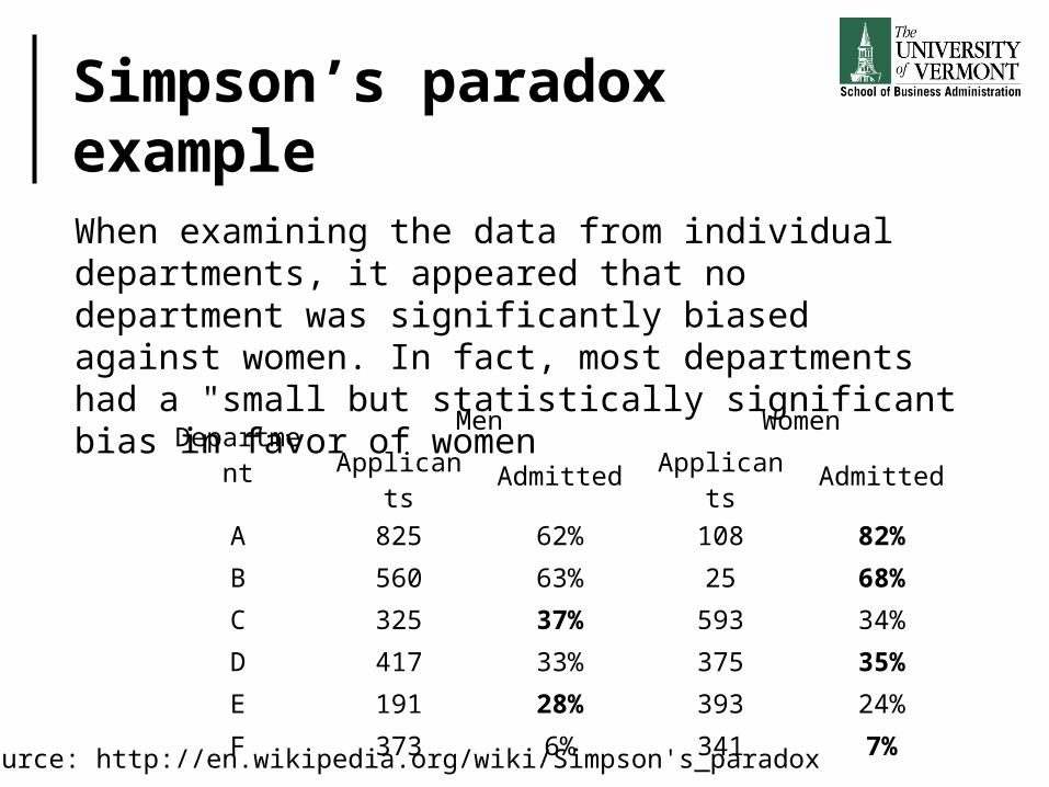
Simpson’s paradox exampleWhen examining the data from individual departments, it appeared that no department was significantly biased against women. In fact, most departments had a "small but statistically significant bias in favor of women


DepartmentMen Women

Applicants Admitted Applicants Admitted

A 825 62% 108 82%

B 560 63% 25 68%

C 325 37% 593 34%

D 417 33% 375 35%

E 191 28% 393 24%

F 373 6% 341 7%

Simpson’s paradox exampleWhat was happening?

Women tended to apply to more competitive departments with low rates of admission even among qualified applicants, whereas men tended to apply to less-competitive departments with high rates of admission among the qualified applicants

The data from specific departments constitute a proper defense against charges of discrimination


Summary

Experiments and the Sample Space Assigning Probabilities to Experimental

OutcomesClassicalRelative frequencySubjective

Events and Their Probabilities

Summary

Some Basic Relationships of Probability1) Compliment of an event2) Addition law3) Conditional probabilities4) Multiplication lawThere are a number of terms to know!

Bayes’ theorem – what is it? Simpson’s paradox – what is it?

Documents

Introduction to probability BSAD 30 Dave Novak Source: Anderson et al., 2013 Quantitative Methods for Business 12 th edition – some slides are directly