Introduction to Probability and Statisticspeople.stfx.ca/asarhan/Stat 224/Notes/chapter3 F10.pdf · Introduction to Probability and Statistics Slides 3 – Chapter 3 Ammar M. Sarhan,

Introduction to Probability and Statistics

Slides 3 – Chapter 3

Ammar M. Sarhan,

[email protected]

Department of Mathematics and Statistics,

Dalhousie University

Fall Semester 2008

Dr. Ammar M. Sarhan 2

Chapter 3

Discrete Random Variables

and

Probability Distributions


Chapter Outlines

3.1 Random Variable

3.2 Probability Distribution for Discrete Random Variables

3.3 Expected Value of Discrete Random variables

3.4 Binomial Distribution

3.5 Hypergeometric & Negative Distributions

3.6 Poisson Distribution

3.1 Random Variables In a statistical experiment, it is often very important to allocate

numerical values to the outcomes.

Example:

• Experiment: testing two components

(D=defective, N=non-defective)

• Sample space: S={DD,DN,ND,NN}

• Let X = number of defective components.

• Assigned numerical values to the outcomes are:

Notice that, the set of all possible values of the variable X is {0, 1, 2}.


Random Variable

For a given sample space S of some experiment, a random variable is

any rule (function) that associates a real number with each outcome in S.

Notation: " X " denotes the random variable .

" x " denotes a particular value of the random variable X.

Bernoulli Random Variable

Any random variable whose only possible values are 0 and 1 is called

a Bernoulli random variable.


A random variable X is called a discrete random variable if its set of

possible values is countable, i.e., x ∈ {x1, x2,…}

Types of Random Variables:

A random variable X is called a continuous random variable if it can

take values on a continuous scale, i.e., x ∈ {x: a < x < b; a, b ∈ R}

A continuous random variable represents measured data, such as

height.

In most practical problems:

A discrete random variable represents count data, such as the

number of defectives in a sample of k items.


3.2 Probability Distributions for Discrete Random Variables

Probability Distribution

The probability distribution or probability mass function (pmf) of a

discrete rv X is defined for every number x by

xXPxsXSsPxp )(:all)(

The probability mass function, p(x), of a discrete random variable X

satisfies the following:

.0)( xXPxp

.1)( xall

xp

1)

2)

Note:

.)()()(

AxallAxall

xXPxpAP


Parameter of a Probability Distribution

Suppose that p(x) depends on a quantity that can be assigned any

one of a number of possible values, each with different value

determining a different probability distribution.

Such a quantity is called a parameter of the distribution.

The collection of all distributions for all different parameters is called

a family of distributions.

Example: For 0< a < 1,

Each choice of a yields a different pmf.

otherwise

xifa

xifa

axp

0

1

01

);(


Proposition

For any two numbers a and b with a ≤ b

“a–” represents the largest possible X value that is strictly less than a.

P(a ≤ X ≤ b) = F(b) – F(a-)

Note: For integers

P(a ≤ X ≤ b) = F(b) - F(a -1)

Cumulative Distribution Function

The cumulative distribution function (cdf) F(x) of a discrete rv variable

X with pmf p(x) is defined by

For any number x, F(x) is the probability that the observed value of X

will be at most x.

.)()(:

xyy

ypxXPxF


Probability Distribution for the Random Variable X

A probability distribution for a random variable X:

x -3 -2 -1 0 1 4 6

P(X=x) 0.13 0.16 0.17 0.20 0.16 0.11 0.07

Find:

1)F(x)

2)P(X > 0)

3)P(-2 ≤ X ≤ 1)

4)P(-2 ≤ X < 1)

5)P(-2 < X ≤ 1)

6)P(-3 < X < 1)

x -3 -2 -1 0 1 4 6

F(x) 0.13 0.29 0.46 0.66 0.82 0.93 1.00

1) F(x)

= 1- P(X ≤ 0) =1 - F(0) = 1 - 0.66 = 0.34

= P(-2 ≤ X ≤ 1) = F(1) – F(-2-) = F(1) – F(-3) = 0.69

= P(-2 ≤ X < 1) = F(1-) – F(-2-) = F(0) – F(-3) = 0.53

= P(-2 < X ≤ 1) = F(1) – F(-2) = F(1) – F(-2) = 0.53

= P(-3 < X < 1) = F(1-) – F(-2) = F(0) – F(-2) = 0. 37


x -3 -2 -1 0 1 4 6

F(x) 0.13 0.29 0.46 0.66 0.82 0.93 1.00

x -3 -2 -1 0 1 4 6

P(X=x) 0.13 0.16 0.17 0.20 0.16 0.11 0.07

6 5 4 3 2 1 0 -1 -2 -3

0.1

0.5

1.0

F(x

)


x

x

x

x

x

x

x

x

xF

6if00.1

64if93.0

41if82.0

10if66.0

01if46.0

12if29.0

23if13.0

3if0

)(

x -3 -2 -1 0 1 4 6

F(x) 0.13 0.29 0.46 0.66 0.82 0.93 1.00

The CDF can be written as

x -3 -2 -1 0 1 4 6

P(X=x) 0.13 0.16 0.17 0.20 0.16 0.11 0.07 pmf:

CDF:


Sample point Value of X (x) Probability

HH 2 P(HH) = P(H) P(H) = 1/3×1/3=1/9

HT 1 P(HT) =P(H) P(T) =1/3×2/3 = 2/9

TH 1 P(HT) = P(H) P(T) =1/3×2/3 = 2/9

TT 0 P(TT) = P(T) P(T) = 2/3×2/3 = 4/9

The possible values of X are: 0, 1, and 2.

X is a discrete random variable.

(X=x) p(x) = P(X=x)

(X=0)={TT} 4/9

(X=1)={HT, TH} 2/9 + 2/9 =4/9

(X=2)={HH} 1/9

X 0 1 2 Total

P(X=x) 4/9 4/9 1/9 1.0

Probability distribution of the X

Tossing a non-balance coin 2 times independently.

Sample space: S={HH, HT, TH, TT}.

Suppose P(H) = ½ P(T) P(H) =1/3 and P(T)=2/3.

Let X= number of heads

Example.


P(X<1) = P(X=0)=4/9

= F(1-) = F(0) =4/9

P(X≤1) = P(X=0) + P(X=1) = 4/9+4/9 = 8/9

= F(1) = 8/9

P(X≥0.5) = P(X=1) + P(X=2) = 4/9+1/9 = 5/9

= 1-F(0.5-) = 1-F(0) = 1-4/9 = 5/9

P(X>8) = P(φ) = 0

=1-F(8) = 1-1 = 0

P(X<10) = P(X=0) + P(X=1) + P(X=2) = P(S) = 1

= F(10) = 1

X 0 1 2

F(x) 4/9 8/9 9/9

F(x)

x

x

x

x

xF

2if1

21if9/8

10if9/4

0if0

)(


A shipment of 8 similar microcomputers to a retail outlet contains 3

that are defective and 5 are non-defective. If a school makes a

random purchase of 2 of these computers, find the probability

distribution of the number of defectives .

We need to find the probability distribution of the random variable:

X = the number of defective computers purchased.

Experiment: selecting 2 computers at random out of 8

N(S) = equally likely outcomes

The possible values of X are: x = 0, 1, 2.

Example :


N(X=0)={0D and 2N} =

N(X=1)= {1D and 1N} =

N(X=2)={2D and 1N} =

P(X=0)= P(X=1)=

P(X=2)=


The probability distribution of X

p(x) =

, x =0,1,2.

p(x) = P(X=x)

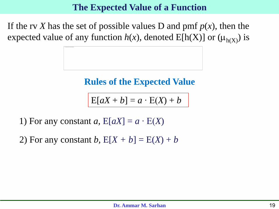
Hypergeometric Distribution

0, otherwise.


3.3 Expected Values of Discrete Random Variables

The Expected Value of X

Let X be a discrete rv with set of possible values D and pmf p(x). The

expected value or mean value of X, denoted E(X) or X or , is

.)()(

Dx

X xpxXE

x 0 1 2 3 4 5 6

p(x) 0.08 0.28 0.38 0.16 0.06 0.03 0.01

Example: Use the data below to find out the expected number of the

number of credit cards that a student will possess.

X = # credit cards

E(X) = x1 p1 + x2 p2 + ... + x6 p6

=0(0.08) +1(0.28)+2(0.38)+3(0.16)+4(0.06)+5( 0.03) + 6(0.01)

=1.97≈ 2 credit cards


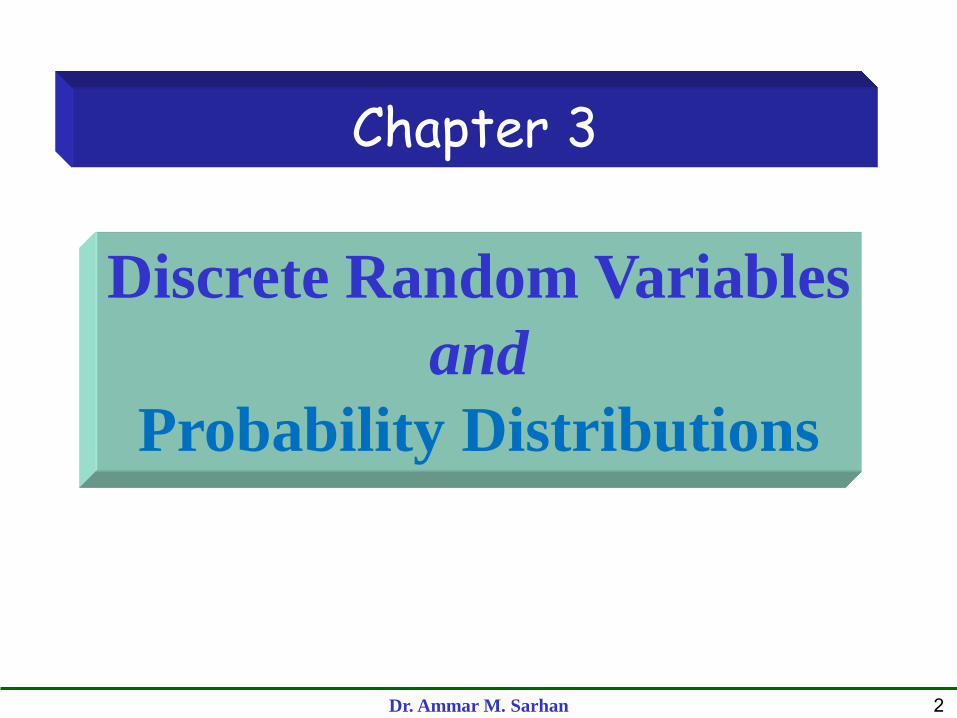
The Expected Value of a Function

If the rv X has the set of possible values D and pmf p(x), then the

expected value of any function h(x), denoted E[h(X)] or (h(X)) is

Rules of the Expected Value

E[aX + b] = a ∙ E(X) + b

1) For any constant a, E[aX] = a ∙ E(X)

2) For any constant b, E[X + b] = E(X) + b


The Variance and Standard Deviation

Let X have pmf p(x), and expected value . Then the variance of X,

denoted V(X) (or or σ2), is

.)()(])[()( 22

Dx

xpxXEXV

2

X

The standard deviation (SD) of X is

2

XX


Example: The quiz scores for a particular student are given below:

22, 25, 20, 18, 12, 20, 24, 20, 20, 25, 24, 25, 18

Value (X) 12 18 20 22 24 25

Frequency 1 2 4 1 2 3

Probability 0.08 0.15 0.31 0.08 0.15 0.23

Compute the variance and standard deviation.

Solution: Let X be the quiz score.

21)( Dx

xpx

p(x)

nn pxpxpxXV 2

1

2

11

2

1 )(...)()()(

31.0)2120(15.0)2118(08.0)2112( 222

25.1323.0)2125(15.0)2124(08.0)2122( 222

64.325.13)( XV


Shortcut Formula for Variance

Rules of Variance


3.4 The Binomial Probability Distribution

Binomial Experiment

An experiment for which the following four conditions are satisfied is

called a binomial experiment.

The experiment consists of a sequence of n trials, where n is fixed

in advance of the experiment.

The probability of success is constant from trial to trial: denoted by p.

The trials are identical, and each trial can result in one of the same

two possible outcomes, which are denoted by success (S) or failure

(F).

The trials are independent

1.

2.

3.

4.


Binomial Random Variable

Given a binomial experiment consisting of n trials, the binomial

random variable X associated with this experiment is defined as

X = the number of S’s among n trials.

Notation for the pmf of a Binomial rv

Because the pmf of a binomial rv X depends on the two parameters n

and p, we denote the pmf by b(x;n,p).

Computation of a Binomial pmf

otherwise0

,,1,0)1(),;(

nxppx

n

pnxbxnx

The expected value and Variance of a Binomial distribution

(1) E(X) = n p (2) V(X) = n p (1- p) If X ~ b(x;n,p)


25

Example: If the probability of a student successfully passing this course

(C or better) is 0.82, find the probability that given 8 students

a. all 8 pass.

c. at least 6 pass.

b. none pass.

2044.0)82.01()82.0(8

8)82.0,8;8()8( 888

bXP

0000011.0)82.01()82.0(0

8)82.0,8;0()0( 080

bXP

)82.0,8;8()82.0,8;7()82.0,8;6()6( bbbXP

787686 )82.01()82.0(7

8)82.01()82.0(

6

8

8392.0)82.01()82.0(8

8888


26

d. The expected number of students passed the course.

e. The variance.

E(X) = n p = 8 (0.82) = 6.56 ≈ 7 students

V(X) = n p (1- p)

= 8 (0.82) (1- 0.82) = 8 (0.82) (0.18)

= 1.1808


27

The Hypergeometric Distribution

3.5 Hypergeometric and Negative Binomial Distributions

The three assumptions that lead to a hypergeometric distribution:

The population or set to be sampled consists of N individuals,

objects, or elements (a finite population).

Each individual can be characterized as a success (S) or failure (F),

and there are M successes in the population.

A sample of n individuals is selected without replacement in such a

way that each subset of size n is equally likely to be chosen.

If X is the number of S’s in a completely random sample of size n

drawn from a population consisting of M S’s and (N – M) F’s, then

the probability distribution of X will be called the hypergeometric

distribution. [ h (n,M,N) ]

1.

2.

3.


Dr. Ammar Sarhan 28

Computation of a Hypergeometric distribution

,),,;()(

n

N

xn

MN

x

M

NMnxhxXP

The expected value and Variance of a Hypergeometric distribution

(1) (2)

If X ~ h (n,M,N)

),min(),0max( MnxMNn

N

MnXE )(

N

M

N

Mn

N

nNXV 1

1)(

N

n

M N-M

x n-x

x

M

xn

MN

n

N


29

Example:

Lots of 40 components each are called acceptable if they contain no

more than 3 defectives. The procedure for sampling the lot is to select 5

components at random (without replacement) and to reject the lot if a

defective is found. What is the probability that exactly one defective is

found in the sample if there are 3 defectives in the entire lot.

Let X= number of defectives in the sample.

Solution: 40

5

3 37

x 5-x

x

3

x5

340

5

40

N = 40, M = 3, n = 5.

X ~ h(n, M, N) ≡ h(5, 3, 40)

,

5

40

5

373

)(

xx

xXP

3)3,5min(0)375,0max( x

x = 0, 1, 2, 3


Dr. Ammar Sarhan 30

The probability that exactly one defective is found in the sample is

P(X= 1) =

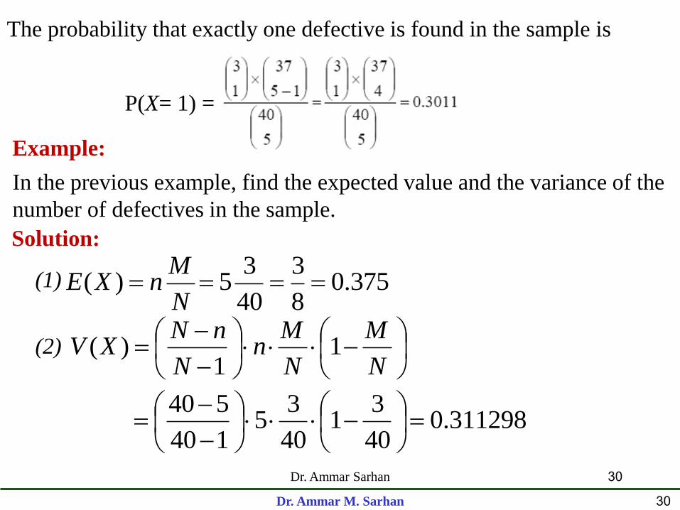
Example:

In the previous example, find the expected value and the variance of the

number of defectives in the sample.

Solution:

(1)

(2)

.37508

3

40

35)(

N

MnXE

N

M

N

Mn

N

nNXV 1

1)(

0.31129840

31

40

35

140

540


31

The Negative Binomial Distribution

The negative binomial rv and distribution are based on an experiment

satisfying the following four conditions:

The experiment consists of a sequence of independent trials.

Each trial can result in a success (S) or a failure (F).

The probability of success is constant from trial to trial, so

P(S on trial i) = p for i = 1, 2, 3, …

The experiment continues until a total of r successes have been

observed, where r is a specified positive integer.

1.

2.

3.

4.

If X is the number of failures that precede the r-th success, then the

probability distribution of X will be called the negative binomial

distribution. [ nb (r, p) ]

The event (X = x) is equivalent to {r-1 S’s in the first (x+r-1) trials and

an S in the (x+r)th}.


32

Computation of a Negative Binomial pmf

,2,1,0,)1(1

1),;(

xpp

r

rxprxnb xr

The expected value and Variance of a Negative Binomial distribution

If X ~ nb(r, p) (1) E(X) = r (1-p)/p (2) V(X) = r (1-p)/p2

Geometric Distribution:

When r = 1 in nb(r, p) then the nb distribution reduces to geometric

distribution.


Example:

Suppose that p=P(male birth) = 0.5. A parent wishes to have exactly

two female children in their family. They will have children until this

condition is fulfilled.

What is the probability that the family has x male children? 1.

What is the probability that the family has 4 children? 2.

What is the probability that the family has at most 4 children? 3.

Let X be the number of Ms precede the 2nd F. X ~ nb(2, 0.5)

The prob. that the family has x male children = P(X=x)

= nb(x; 2,0.5), x=0,1,2,...

= P(X = 2) = nb(2; 2, 0.5) = 0.1875

= P(X ≤ 2 ) = P(X = 0) + P(X = 1) + P(X = 2)

= nb(0; 2, 0.5) + nb(1; 2, 0.5) + nb(2; 2, 0.5)

= 0.6875


How many male children would you expect this family to have?

How many children would you expect this family to have?

4.

E(X) = r (1 – p)/ p = 2 (1-0.5) / 0.5 = 2

2 + E(X) = 2 + 2 = 4


3.6 The Poisson Probability Distribution

A random variable X is said to have a Poisson distribution with

parameter λ (λ > 0), if the pmf of X is

,2,1,0,!

);(

xx

exp

x

The Poisson Distribution as a Limit

Suppose that in the binomial pmf b(x;n, p), we let n → ∞ and p → 0

in such a way that np approaches a value λ (λ > 0). Then

b(x; n, p) → p(x; λ)

The expected value and Variance of a Poisson distribution

E(X) = V(X) = λ

If X has a Poisson distribution with parameter λ , then


Poisson Process

Assumptions:

Pk (t) = e- αt (αt)k / k! , so that the number of pulses (events) during a

time interval of length t is a Poisson rv with parameter αt. The expected

number of pulses (events) during any such time interval is αt, so the

expected number during a unit time interval is α.

Poisson Process

There exists a parameter α > 0 such that for any short time interval of

length Δt , the probability that exactly one event is received is

α Δt + o(Δt )

1.

The probability of more than one event during Δt is o(Δt ). 2.

The number of events during the time interval Δt is independent of

the number that occurred prior to this time interval.

3.


Example:

Suppose that the number of typing errors per page has a Poisson

distribution with average 6 typing errors.

(1) What is the probability that in a given page:

(i) The number of typing errors will be 7?

(ii) The number of typing errors will be at least 2?

Let X = number of typing errors per page. X ~ Poisson (6)

.13768.0!7

6)6;7()7(

67

e

pXP(i)

,2,1,0,!

6)6;()(

6

xx

expxXP

x

)1()0(1)2(1)2( XPXPXPXP(ii)

=1 - p(0; 6) – p(1; 6) = 0.982650


(2) What is the probability that in 2 pages there will be 10 typing errors?

X ~ Poisson (12) Let X = number of typing errors in 2 pages.

.1084.0!10

12)12;10()10(

1210

e

pXP

(3) What is the probability that in a half page there will be no typing

errors?

Let X = number of typing errors in a half page. X ~ Poisson (3)

. 0.0497871!0

3)3;0()0(

30

e

pXP

Documents

Introduction to Probability and Statisticspeople.stfx.ca/asarhan/Stat 224/Notes/chapter3 F10.pdf · Introduction to Probability and Statistics Slides 3 – Chapter 3 Ammar M. Sarhan,