Embed Size (px)
Citation preview
Massachusetts Institute of Technology Course Notes 106.042J/18.062J, Fall ’02: Mathematics for Computer ScienceProfessor Albert Meyer and Dr. Radhika Nagpal
Introduction to Probability
1 Probability
Probability will be the topic for the rest of the term. Probability is one of the most important subjects in Mathematics and Computer Science. Most upper level Computer Science courses require probability in some form, especially in analysis of algorithms and data structures, but also in information theory, cryptography, control and systems theory, network design, artificial intelligence, and game theory. Probability also plays a key role in fields such as Physics, Biology, Economics and Medicine.
There is a close relationship between Counting/Combinatorics and Probability. In many cases, the probability of an event is simply the fraction of possible outcomes that make up the event. So many of the rules we developed for finding the cardinality of finite sets carry over to Probability Theory. For example, we’ll apply an Inclusion-Exclusion principle for probabilities in some examples below.
In principle, probability boils down to a few simple rules, but it remains a tricky subject because these rules often lead unintuitive conclusions. Using “common sense” reasoning about probabilistic questions is notoriously unreliable, as we’ll illustrate with many real-life examples.
This reading is longer than usual . To keep things in bounds, several sections with illustrative examples that do not introduce new concepts are marked “[Optional].” You should read these sections selectively, choosing those where you’re unsure about some idea and think another ex-ample would be helpful.
2 Modelling Experimental Events
One intuition about probability is that we want to predict how likely it is for a given experiment to have a certain kind of outcome. Asking this question invariably involves four distinct steps:
Find the sample space. Determine all the possible outcomes of the experiment.
Define the event of interest. Determine which of those possible outcomes is “interesting.”
Determine the individual outcome probabilities. Decide how likely each individual outcome is to occur.
Determine the probability of the event. Combine the probabilities of “interesting” outcomes to find the overall probability of the event we care about.
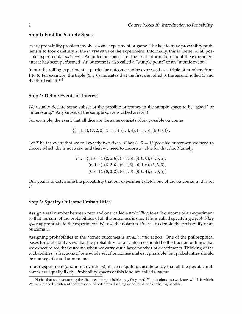
In order to understand these four steps, we will begin with a toy problem. We consider rolling three dice, and try to determine the probability that we roll exactly two sixes.
Copyright © 2002, Prof. Albert R. Meyer.
2 Course Notes 10: Introduction to Probability
Step 1: Find the Sample Space
Every probability problem involves some experiment or game. The key to most probability problems is to look carefully at the sample space of the experiment. Informally, this is the set of all possible experimental outcomes. An outcome consists of the total information about the experiment after it has been performed. An outcome is also called a “sample point” or an “atomic event”.
In our die rolling experiment, a particular outcome can be expressed as a triple of numbers from 1 to 6. For example, the triple (3, 5, 6) indicates that the first die rolled 3, the second rolled 5, and the third rolled 6.1
Step 2: Define Events of Interest
We usually declare some subset of the possible outcomes in the sample space to be “good” or “interesting.” Any subset of the sample space is called an event.
For example, the event that all dice are the same consists of six possible outcomes
{(1, 1, 1), (2, 2, 2), (3, 3, 3), (4, 4, 4), (5, 5, 5), (6, 6, 6)} .
Let T be the event that we roll exactly two sixes. T has 3 · 5 = 15 possible outcomes: we need to choose which die is not a six, and then we need to choose a value for that die. Namely,
T ::= {(1, 6, 6), (2, 6, 6), (3, 6, 6), (4, 6, 6), (5, 6, 6), (6, 1, 6), (6, 2, 6), (6, 3, 6), (6, 4, 6), (6, 5, 6), (6, 6, 1), (6, 6, 2), (6, 6, 3), (6, 6, 4), (6, 6, 5)}
Our goal is to determine the probability that our experiment yields one of the outcomes in this set T .
Step 3: Specify Outcome Probabilities
Assign a real number between zero and one, called a probability, to each outcome of an experiment so that the sum of the probabilities of all the outcomes is one. This is called specifying a probability space appropriate to the experiment. We use the notation, Pr {w}, to denote the probability of an outcome w.
Assigning probabilities to the atomic outcomes is an axiomatic action. One of the philosophical bases for probability says that the probability for an outcome should be the fraction of times that we expect to see that outcome when we carry out a large number of experiments. Thinking of the probabilities as fractions of one whole set of outcomes makes it plausible that probabilities should be nonnegative and sum to one.
In our experiment (and in many others), it seems quite plausible to say that all the possible out-comes are equally likely. Probability spaces of this kind are called uniform:
1Notice that we’re assuming the dice are distinguishable—say they are different colors—so we know which is which. We would need a different sample space of outcomes if we regarded the dice as indistinguishable.
�
Course Notes 10: Introduction to Probability 3
Definition 2.1. A uniform probability space is a finite space in which all the outcomes have the same probability. That is, if S is the sample space, then
1Pr {w} =
|S|
for every outcome w ∈ S.
Since there are 63 = 216 possible outcomes, we axiomatically declare that each occurs with probability 1/216.
Step 4: Compute Event Probabilities
We now have a probability for each outcome. To compute the probability of the event, T , that we get exactly two sixes, we add up the probabilities of all the outcomes that yield exactly two sixes. In our example, since there are 15 outcomes in T , each with probability 1/216, we can deduce that Pr {T } = 15/216.
Probability on a uniform sample space such as this one is pretty much the same as counting. Another example where it’s reasonable to use a uniform space is for poker hands. Instead of asking how many distinct full houses there are in poker, we can ask about the probability that a “random” poker hand is a full house. For example, of the
�52
� possible poker hands, we saw that5
• There are 624 “four of a kind” hands, so the probability of 4 of a kind is 624/ �52 5 = 1/4165.
• There are 3744 “full house” hands, so the probability of a full house is 6/4165 ≈ 1/694.
• There are 123,552 “two pair” hands, so the probability of two pair ≈ 1/21.
3 The Monty Hall Problem
In the 1970’s, there was a game show called Let’s Make a Deal, hosted by Monty Hall and his assistant Carol Merrill. At one stage of the game, a contestant is shown three doors. The contestant knows there is a prize behind one door and that there are goats behind the other two. The contestant picks a door. To build suspense, Carol always opens a different door, revealing a goat. The contestant can then stick with his original door or switch to the other unopened door. He wins the prize only if he now picks the correct door. Should the contestant “stick” with his original door, “switch” to the other door, or does it not matter?
This was the subject of an “Ask Marilyn” column in Parade Magazine a few years ago. Marilyn wrote that your chances of winning were 2/3 if you switched — because if you switch, then you win if the prize was originally behind either of the two doors you didn’t pick. Now, Marilyn has been listed in the Guiness Book of World Records as having the world’s highest IQ, but for this answer she got a tidal wave of critical mail, some of it from people with Ph.D.’s in mathematics, telling her she was wrong. Most of her critics insisted that the answer was 1/2, on the grounds that the prize was equally likely to be behind each of the doors, and since the contestant knew he was going to see a goat, it remains equally likely which the two remaining doors has the prize behind it. The pros and cons of these arguments still stimulate debate.
4 Course Notes 10: Introduction to Probability
It turned out that Marilyn was right, but given the debate, it is clearly not apparent which of the intuitive arguments for 2/3 or 1/2 is reliable. Rather than try to come up with our own explanation in words, let’s use our standard approach to finding probabilities. In particular, we will analyze the probability that the contestant wins with the “switch” strategy; that is, the contestant chooses a random door initially and then always switches after Carol reveals a goat behind one door. We break the down into the standard four steps.
Step 1: Find the Sample Space
In the Monty Hall problem, an outcome is a triple of door numbers:
1. The number of the door concealing the prize.
2. The number of the door initially chosen by the contestant.
3. The number of the door Carol opens to reveal a goat.
For example, the outcome (2, 1, 3) represents the case where the prize is behind door 2, the contestant initially chooses door 1, and Carol reveals the goat behind door 3. In this case, a contestant using the “switch” strategy wins the prize.
Not every triple of numbers is an outcome; for example, (1, 2, 1) is not an outcome, because Carol never opens the door with the prize. Similarly, (1, 2, 2) is not an outcome, because Carol does not open the door initially selected by the contestant, either.
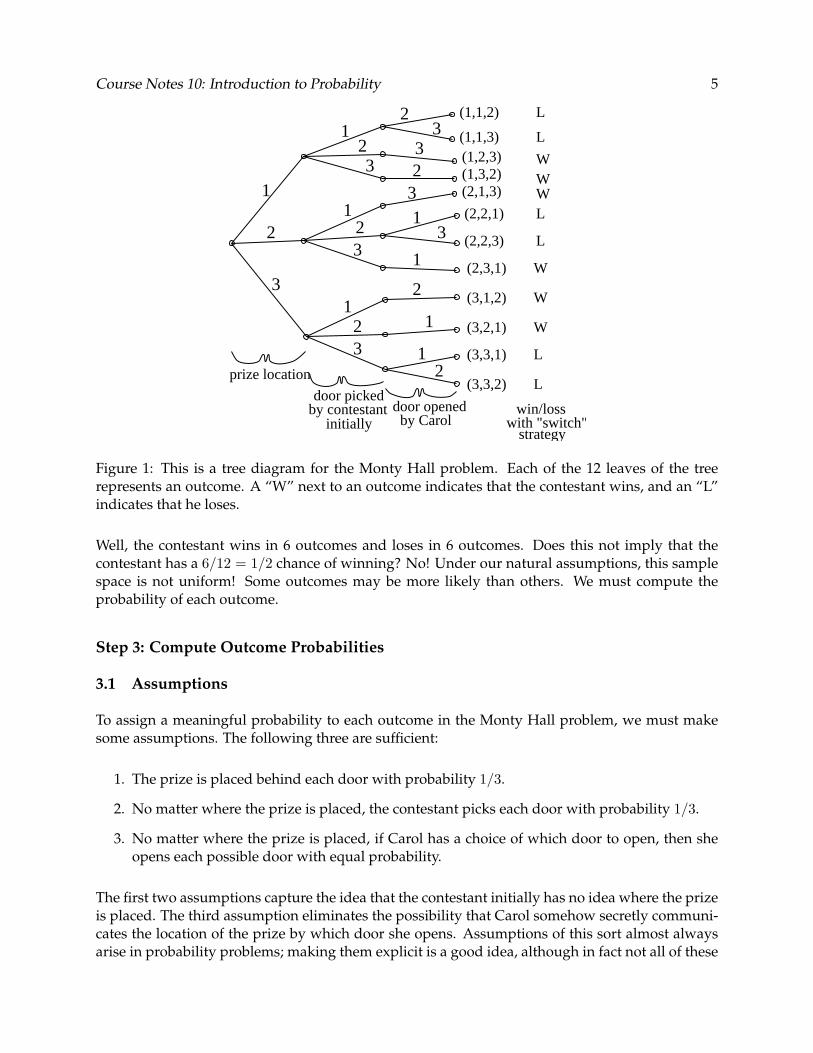
As with counting, a tree diagram is a standard tool for studying the sample space of an experiment. The tree diagram for the Monty Hall problem is shown in Figure 1. Each vertex in the tree corresponds to a state of the experiment. In particular, the root represents the initial state, before the prize is even placed. Internal nodes represent intermediate states of the experiment, such as after the prize is placed, but before the contestant picks a door. Each leaf represents a final state, an outcome of the experiment. One can think of the experiment as a walk from the root (initial state) to a leaf (outcome). In the figure, each leaf of the tree is labeled with an outcome (a triple of numbers) and a “W” or “L” to indicate whether the contestant wins or loses.
Step 2: Define Events of Interest
For the Monty Hall problem, let S denote the sample space, the set of all 12 outcomes shown in Figure 1. The event W ⊂ S that the contestant wins with the “switch” strategy consists of six outcomes:
W ::= {(1, 2, 3), (1, 3, 2), (2, 1, 3), (2, 3, 1), (3, 1, 2), (3, 2, 1)} .
The event L ⊂ S that the contestant loses is the complementary set:
L ::= {(1, 1, 2), (1, 1, 3), (2, 2, 1), (2, 2, 3), (3, 3, 1), (3, 3, 2)} .
Our goal is to determine the probability of the event W ; that is, the probability that the contestant wins with the “switch” strategy.
Course Notes 10: Introduction to Probability 5
1
12
3
2
3
23
32
1
1
2
2
3
3
31
3
1
2
1
12
(3,3,2)
(3,3,1)
(3,2,1)
(3,1,2)
(2,3,1)
(2,2,3)
(1,1,2)
(1,1,3)(1,2,3)(1,3,2)(2,1,3)
(2,2,1)
door pickedby contestant door opened
by Carol
prize location
initially
WW
L
L
WL
L
W
W
W
L
L
win/losswith "switch"
strategy
Figure 1: This is a tree diagram for the Monty Hall problem. Each of the 12 leaves of the tree represents an outcome. A “W” next to an outcome indicates that the contestant wins, and an “L” indicates that he loses.
Well, the contestant wins in 6 outcomes and loses in 6 outcomes. Does this not imply that the contestant has a 6/12 = 1/2 chance of winning? No! Under our natural assumptions, this sample space is not uniform! Some outcomes may be more likely than others. We must compute the probability of each outcome.
Step 3: Compute Outcome Probabilities
3.1 Assumptions
To assign a meaningful probability to each outcome in the Monty Hall problem, we must make some assumptions. The following three are sufficient:
1. The prize is placed behind each door with probability 1/3.
2. No matter where the prize is placed, the contestant picks each door with probability 1/3.
3. No matter where the prize is placed, if Carol has a choice of which door to open, then she opens each possible door with equal probability.
The first two assumptions capture the idea that the contestant initially has no idea where the prize is placed. The third assumption eliminates the possibility that Carol somehow secretly communicates the location of the prize by which door she opens. Assumptions of this sort almost always arise in probability problems; making them explicit is a good idea, although in fact not all of these
6 Course Notes 10: Introduction to Probability
assumptions are absolutely necessary. For example, it doesn’t matter how Carol chooses a door to open in the cases when she has a choice, though we won’t prove this.
3.2 Assigning Probabilities to Outcomes
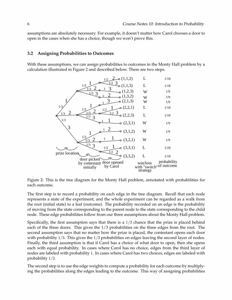
With these assumptions, we can assign probabilities to outcomes in the Monty Hall problem by a calculation illustrated in Figure 2 and described below. There are two steps.
1
3
32
1
2
1
(3,3,2)
(3,3,1)
(3,2,1)
(3,1,2)
(2,3,1)
(2,2,3)
(1,1,2)
(1,1,3)(1,2,3)(1,3,2)(2,1,3)
(2,2,1)
door pickedby contestant door opened
by Carol
prize location
initially
WW
L
L
WL
L
W
W
W
L
L
win/losswith "switch"
strategy
1/3
1/3
1/3
1/31/3
1/3
1/31/31/3
1/31/31/3
1/2
1/21/2
1/21/2
1
1
1
1
1
1
1/18
1/18
1/9
1/9
1/9
1/18
1/18
1/9
1/9
1/9
1/18
1/18
probabilityof outcome
1/2
13
21
23
32
1
32
12
21
33
Figure 2: This is the tree diagram for the Monty Hall problem, annotated with probabilities for each outcome.
The first step is to record a probability on each edge in the tree diagram. Recall that each node represents a state of the experiment, and the whole experiment can be regarded as a walk from the root (initial state) to a leaf (outcome). The probability recorded on an edge is the probability of moving from the state corresponding to the parent node to the state corresponding to the child node. These edge probabilities follow from our three assumptions about the Monty Hall problem.
Specifically, the first assumption says that there is a 1/3 chance that the prize is placed behind each of the three doors. This gives the 1/3 probabilities on the three edges from the root. The second assumption says that no matter how the prize is placed, the contestant opens each door with probability 1/3. This gives the 1/3 probabilities on edges leaving the second layer of nodes. Finally, the third assumption is that if Carol has a choice of what door to open, then she opens each with equal probability. In cases where Carol has no choice, edges from the third layer of nodes are labeled with probability 1. In cases where Carol has two choices, edges are labeled with probability 1/2.
The second step is to use the edge weights to compute a probability for each outcome by multiplying the probabilities along the edges leading to the outcome. This way of assigning probabilities
Course Notes 10: Introduction to Probability 7
reflects our idea that probability measures the fraction of times that a given outcome should hap-pen over the course of many experiments. Suppose we want the probability of outcome (2, 1, 3). In 1/3 of the experiments, the prize is behind the second door. Then, in 1/3 of these experiments when the prize is behind the second door, and the contestant opens the first door. After that, Carol has no choice but to open the third door. Therefore, the probability of the outcome is the product of the edge probabilities, which is
1 1 1 3 · 3 · 1 =
9 .
For example, the probability of outcome (2, 2, 3) is the product of the edge probabilities on the path from the root to the leaf labeled (2, 2, 3). Therefore, the probability of the outcome is
1 1 1 1 =
3 · 3 · 2 18
.
Similarly, the probability of outcome (3, 1, 2) is
1 1 1 3 · 3 · 1 =
9 .
The other outcome probabilities are worked out in Figure 2.
Step 4: Compute Event Probabilities
We now have a probability for each outcome. All that remains is to compute the probability of W , the event that the contestant wins with the “switch” strategy. The probabilility of an event is simply the sum of the probabilities of all the outcomes in it. So the probability of the contestant winning with the “switch” strategy is the sum of the probabilities of the six outcomes in event W , namely, 2/3:
Pr {W } ::= Pr {(1, 2, 3)} + Pr {(1, 3, 2)} + Pr {(2, 1, 3)} + Pr {(2, 3, 1)} + Pr {(3, 1, 2)} + Pr {(3, 2, 1)} 1 1 1 1 1 1
= 9
+9
+9
+9
+9
+9
2 =
3 .
In the same way, we can compute the probability that a contestant loses with the “switch” strategy. This is the probability of event L:
Pr {L} ::= Pr {(1, 1, 2)} + Pr {(1, 1, 3)} + Pr {(2, 2, 1)} + Pr {(2, 2, 3)} + Pr {(3, 3, 1)} + Pr {(3, 3, 2)} 1 1 1 1 1 1
= 18
+ 18
+ 18
+ 18
+ 18
+ 18
1 =
3 .
The probability of the contestant losing with the switch strategy is 1/3. This makes sense; the probability of winning and the probability of losing ought to sum to 1!
We can determine the probability of winning with the “stick” strategy without further calculations. In every case where the “switch” strategy wins, the “stick” strategy loses, and vice versa. Therefore, the probability of winning with the stick strategy is 1 − 2/3 = 1/3.
Solving the Monty Hall problem formally requires only simple addition and multiplication. But trying to solve the problem with “common sense” leaves us running in circles!
8 Course Notes 10: Introduction to Probability
4 Intransitive Dice
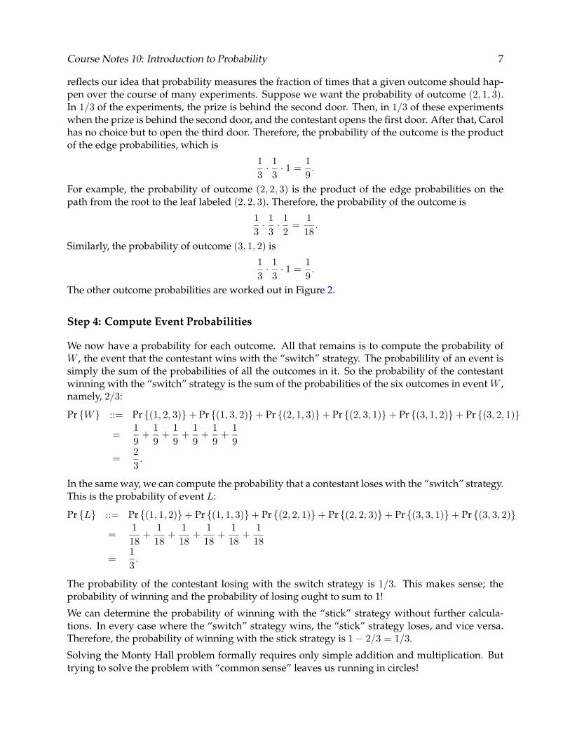
There is a game involving three dice and two players. The dice are not normal; rather, they are numbered as shown in Figure 3. Each hidden face has the same number as the opposite, exposed face. As a result, each die has only three distinct numbers, and each number comes up 1/3 of the time.
BA C
2 1 3
6 7 5 9 4 8
Figure 3: This figure shows the strange numbering of the three dice “intransitive” dice. The number on each concealed face is the same as the number on the exposed, opposite face.
In the game, the first player can choose any one of the three dice. Then the second player chooses one of the two remaining dice. They both roll and the player with the higher number wins. Which of the three dice should player one choose? That is, which of the three dice is best?
For example, die B is attractive, because it has a 9, the highest number overall; on the other hand, it also has a 1, the lowest number. Intuition gives no clear answer! We can solve the problem with our standard four-step method.
Claim 4.1. Die A beats die B more than half of the time.
Proof. The claim concerns the experiment of throwing dice A and B.
Step 1: Find the Sample Space. The sample space for this experiment is indicated by the tree diagram in Figure 4.
Step 2: Define Events of Interest. We are interested in the event that die A comes up greater than die B. The outcomes in this event are marked “A” in the figure.
Step 3: Compute Outcome Probabilities. To find outcome probabilities, we first assign probabilities to edges in the tree diagram. Each number comes up with probability 1/3, regardless of the value of the other die. Therefore, we assign all edges probability 1/3. The probability of an outcome is the product of probabilities on the corresponding root-to-leaf path; this means that every outcome has probability 1/9.
Step 4: Compute Event Probabilities. The probability of an event is the sum of the probabilities of the outcomes in the event. Therefore, the probability that die A comes up greater than die “B” is
1 1 1 1 1 5 =
9+
9+
9+
9+
9 9 .
As claimed, the probability that die A beats die B is greater than half.
Course Notes 10: Introduction to Probability 9
1/31/3
1/3
1/3
1/3
1/3
1/3
1/3
1/3
1/3
1/3
1/3
2
6
7
15
9
1
1
5
5
9
9
die A die B
B
B
B
B
A
A
A
A
A
winner probabilityof outcome
1/9
1/9
1/9
1/9
1/9
1/9
1/9
1/9
1/9
A wins withprobability 5/9
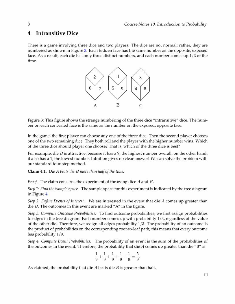
Figure 4: This is the tree diagram arising when die A is played against die B. Die A beats die B with probability 5/9.
The analysis may be even clearer by giving the outcomes in a table:
Winner B roll 1 5 9
A roll 2 A B B 6 A A B 7 A A B
All the outcomes are equally likely, and we see that A wins 5 of them. This table works because our probability space is based on 2 pieces of information, A’s roll and B’s roll. For more complex probability spaces, the tree diagram is necessary.
Claim 4.2. Die B beats die C more than half of the time.
Proof. The proof is by the same case analysis as for the preceding claim, summarized in the table:
Winner C roll 3 4 8
B roll 1 C C C 5 B B C 9 B B B
10 Course Notes 10: Introduction to Probability
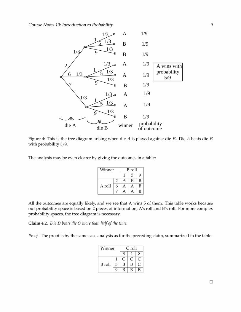
We have shown that A beats B and that B beats C. From these results, we might conclude that A is the best die, B is second best, and C is worst. But this is totally wrong!
Claim 4.3. Die C beats die A more than half of the time!
Proof. See the tree diagram in Figure 5. Again, we can present this analysis in a tabular form:
Winner A roll 2 6 7
C roll 3 C A A 4 C A A 8 C C C
1/31/3
1/3
1/3
1/3
1/3
1/3
1/3
1/3
1/3
1/3
1/3
winner probabilityof outcome
1/9
1/9
1/9
1/9
1/9
1/9
1/9
1/9
1/9
probability 5/9
die C die A
4
8
3
2
2
2
7
7
7
6
6
6
A
C wins withA
C
C
A
A
C
C
C
Figure 5: Die C beats die A with probability 5/9. Amazing!
Die A beats B, B beats C, and C beats A! Apparently, there is no “transitive law” here! This means that no matter what die the first player chooses, the second player can choose a die that beats it with probability 5/9. The player who picks first is always at a disadvantage!
[Optional]
The same effect can arise with three dice numbered the ordinary way, but “loaded” so that some numbers turn up more often. For example, suppose:
Course Notes 10: Introduction to Probability 11
A rolls 3 with probability 1
√ B rolls 2 with probability p ::= ( 5 − 1)/2 = 0.618 . . .
rolls 5 with probability 1 − p
C rolls 1 with probability 1 − p
rolls 4 with probability p
It’s clear that A beats B, and C beats A, each with probability p. But note that 1 − p 2 = p. Now the probability that B beats C is
2Pr {B rolls to 5} + Pr {B rolls to 2 and C rolls to 1} = (1 − p) + p(1 − p) = 1 − p = p.
So A beats B, B beats C, and C beats A, all with probability p = 0.618 · · · > 5/9.
5 Set Theory and Probability
Having gone through these examples, we should be ready to make sense of the formal definitions of basic probability theory.
5.1 Basic Laws of Probability
Definition 5.1. A sample space, S, is a nonempty set whose elements are called outcomes. The events are subsets of S.2
Definition. A family, F , of sets is pairwise disjoint if the intersection of every pair of distinct sets � in the family is empty, i.e., if A,B ∈ F and A �= B, then A ∩ B = ∅. In this case, if S = F , then S is said to be the disjoint union of the sets in F .
Definition 5.2. A probability space consists of a sample space, S, and a probability function, Pr {}, mapping the events of S to real numbers between zero and one, such that:
1. Pr {S} = 1, and 2 For all the examples in 6.042, we let every subset of S be an event. However, when S is a set such as the unit
interval of real numbers, there can be problems. In this case, we typically want subintervals of the unit interval to be events with probability equal to their length. For example, we’d say that if a dart hit “at random” in the unit interval, then the probability that it landed within the subinterval from 1/3 to 3/4 was equal to the length of the interval, namely 5/12.
Now it turns out to be inconsistent with the axioms of Set Theory to insist that all subsets of the unit interval be events. Instead, the class of events must be limited to rule out certain pathological subsets which do not have a well-defined length. An example of such a pathological set is the real numbers between zero and one with an infinite number of fives in the even-numbered positions of their decimal expansions. Fortunately, such pathological subsets are not relevant in applications of Probability Theory.
The results of the Probability Theory hold as long as we have some set of events with a few basic properties: every finite set of outcomes is an event, the whole space is an event, the complement of an event is an event, and if A0, A1, . . . � are events, so is i∈N Ai . It is easy to come up with such a class of events that includes all the events we care about and leaves out all the pathological cases.
� �
� �
� �
�
12 Course Notes 10: Introduction to Probability
2. if A0, A1, . . . is a sequence of disjoint events, then � Pr Ai = Pr {Ai} . (Sum Rule)
i∈N i∈N
The Sum Rule3 lets us analyze a complicated event by breaking it down into simpler cases. For example, if the probability that a randomly chosen MIT student is native to the United States is 60%, to Canada is 5%, and to Mexico is 5%, then the probability that a random MIT student is native to North America is 70%.
One immediate consequence of Definition 5.2 is that Pr {A} + Pr A = 1 because S is the disjoint union of A and A. This equation often comes up in the form
Pr A = 1 − Pr {A} . (Complement Rule)
Some further basic facts about probability parallel facts about cardinalities of finite sets. In particular:
Pr {B − A} = Pr {B} − Pr {A ∩ B} (Difference Rule) Pr {A ∪ B} = Pr {A} + Pr {B} − Pr {A ∩ B} (Inclusion-Exclusion)
The Difference Rule follows from the Sum Rule because B is the disjoint union of B − A and A ∩ B. The (Inclusion-Exclusion) equation then follows from the Sum and Difference Rules, because A∪B is the disjoint union of A and B − A, so
Pr {A ∪ B} = Pr {A} + Pr {B − A} = Pr {A} + (Pr {B} − Pr {A ∩ B}).
This (Inclusion-Exclusion) equation is the Probability Theory version of the Inclusion-Exclusion Principle for the size of the union of two finite sets. It generalizes to n events in a corresponding way. An immediate consequence of (Inclusion-Exclusion) is
Pr {A ∪ B} ≤ Pr {A} + Pr {B} . (Boole’s Inequality)
Similarly, the Difference Rule implies that
If A ⊆ B, then Pr {A} ≤ Pr {B} . (Monotonicity)
In the examples we considered above, we used the fact that the probability of an event was the sum of the probabilities of its outcomes. This follows as a trivial special case of the Sum Rule with one quibble: according to the official definition, the probability function is defined on events not outcomes. But we can always treat an outcome as the event whose only element is that outcome, that is, define Pr {w} to be Pr {{w}}. Then, for the record, we can say
Corollary 5.3. If A = {w0, w1, . . . } is an event, then
Pr {A} = Pr {wi} . i∈N
3If you think like a Mathematician, you should be wondering if the infinite sum is really necessary. Namely, suppose we had only used finite sums in Definition 5.2 instead of sums over all natural numbers. Would this imply the result for infinite sums? It’s hard to find counterexamples, but there are some: it is possible to find a pathological “probability” measure on a sample space satisfying the Sum Rule for finite unions, in which the outcomes w0, w1 , . . . each have probability zero, and the probability assigned to any event is either zero or one! So the infinite Sum Rule fails dramatically, since the whole space is of measure one, but it is a union of the outcomes of measure zero.
The construction of such weird examples is beyond the scope of 6.042. You can learn more about this by taking a course in Set Theory and Logic that covers the topic of “ultrafilters.”
� �
� � �
� � � � �
�
� � � � �
� � � � � �
�� � � � � �
Course Notes 10: Introduction to Probability 13
5.2 Circuit Failure
Suppose you are wiring up a circuit containing a total of n connections. From past experience we assume that any particular connection is made incorrectly with probability p, for some 0 ≤ p ≤ 1. That is, for 1 ≤ i ≤ n,
Pr {ith connection is wrong} = p.
What can we say about the probability that the circuit is wired correctly, i.e., that it contains no incorrect connections?
Let Ai denote the event that connection i is made correctly. Then Ai is the event that connection i is made incorrectly, so Pr Ai = p. Now
n
i=1
Ai .Pr {all connections are OK} = Pr
Without any additional assumptions, we can’t get an exact answer. However, we can give reason-able upper and lower bounds. For an upper bound, we can see that
Prn
i=1
Ai = Pr A1 ∩ ( ≤ Pr {A1} = 1 − p n
Ai) i=2
by Monotonicity. For a lower bound, we can see that
Prn
i=1
Ai = 1 − Prn
i=1
Ai = 1 − Prn
i=1
Ai ≥ 1 −n
i=1
Pr Ai = 1 − np,
where the ≥-inequality follows from Boole’s Law.
So for example, if n = 10 and p = 0.01, we get the following bounds:
0.9 = 1 − 10 · 0.01 ≤ Pr {all connections are OK} ≤ 1 − 0.01 = 0.99.
So we have concluded that the chance that all connections are okay is somewhere between 90% and 99%. Could it actually be as high as 99%? Yes, if the errors occur in such a way that all connection errors always occur at the same time.
Could it be 90%? Yes, suppose the errors are such that we never make two wrong connections. In other words, the events Ai are all disjoint and the probability of getting it right is
Pr Ai = 1 − Pr�
Ai = 1 −10
i=1
Pr Ai = 1 − 10 · 0.01 = 0.9.
6 Combinations of Events
6.1 Carnival Dice
There is a gambling game called Carnival Dice. A player picks a number between 1 and 6 and then rolls three fair dice—“fair” means each number is equally likely to show up on a die. The
14 Course Notes 10: Introduction to Probability
player wins if his number comes up on at least one die. The player loses if his number does not appear on any of the dice. What is the probability that the player wins? This problem sounds simple enough that we might try an intuitive lunge for the solution.
False Claim 6.1. The player wins with probability 1/2.
False proof. Let Ai be the event that the ith die matches the player’s guess.
Pr {win} = Pr {A1 ∪ A2 ∪ A3} (1) = Pr {A1} + Pr {A2} + Pr {A3} (2)
1 1 1 =
6+
6+
6 (3)
1 =
2 (4)
The justification for the equality (2) is that the union is disjoint. This may seem reasonable in a vague way, but in a precise way it’s not. To see that this is a silly argument, note that it would also imply that with six dice, our probability of getting a match is 1, i.e., it is sure to happen. This is clearly false—there is some chance that none of the dice match.4
To compute the actual chance of winning at Carnival Dice, we can use Inclusion-Exclusion for three sets. The probability that one die matches the player’s guess is 1/6. The probability that two particular dice both match the player’s guess is 1/36: there are 36 possible outcomes of the two dice and exactly one of them has both equal to the player’s guess. The probability that all three dice match is 1/216. Inclusion-Exclusion gives:
1 1 1 1 1 1 1 91Pr {win} =
6+
6+
6 −
36 −
36 −
36+
216 =
216 ≈ 42%.
These are terrible odds in a gambling game; it is much better to play roulette, craps, or blackjack!
6.2 More Intransitive Dice [Optional]
[Optional]
In Section 4, we√described three dice A, B and C such that the probabilities of A beating B, B beating C, C beating A are each p ::= ( 5 − 1)/2 ≈ 0.618. Can we increase this probability? For example, can we design dice so that each of these probabilities are, say, at least 3/4? The answer is “No.” In fact, using the elementary rules of probability, it’s easy to show that these “beating” probabilities cannot all exceed 2/3.
In particular, we consider the experiment of rolling all three dice, and define [A] to be the event that A beats B, [B] the event that B beats C, and [C] the event that C beats A.
Claim.
2 min {Pr {[A]} , Pr {[B]} , Pr {[C]}} ≤
3 . (5)
4On the other hand, the idea of adding these probabilities is not completely absurd. We will see in Course Notes 11 that adding would work to compute the average number of matching dice: 1/2 a match per game with three dice and one match per game in the game with six dice.
� �
� �
Course Notes 10: Introduction to Probability 15
Proof. Suppose dice A, B, C roll numbers a, b, c. Events [A], [B], [C] all occur on this roll iff a > b, b > c, c > a, so in fact they cannot occur simultaneously. That is,
[A] ∩ [B] ∩ [C] = ∅. (6)
Therefore,
0 = Pr {[A] ∩ [B] ∩ [C]} (by (6))
=1 − Pr [A] ∪ [B] ∪ [C] (Complement Rule and DeMorgan) � � � � � � ≥1 − (Pr [A] + Pr [B] + Pr [C] (Boole’s Inequality)
= Pr {[A]} + Pr {[B]} + Pr {[C]}) − 2 (Complement Rule)
≥3 min {Pr {[A]} , Pr {[B]} , Pr {[C]}} − 2. (def of min)
Hence
2 ≥ 3min {Pr {[A]} , Pr {[B]} , Pr {[C]}} ,
proving (5).
6.3 Derangements [Optional]
[Optional]
Suppose we line up two randomly ordered decks of n cards against each other. What is the probability that at least one pair of cards “matches”? Let Ai be the event that card i is in the same place in both arrangements. We are interested in� Pr { Ai }. To apply the Inclusion-Exclusion formula, we need to compute the probabilities of individual intersection events—namely, to determine the probability Pr {Ai1 ∩ Ai2 ∩ · · · ∩ Aik } that a particular set of k cards matches. To do so we apply our standard four steps.
The sample space. The sample space involves a permutation of the first card deck and a permutation of the second deck. We can think of this as a tree diagram: first we permute the first deck (n! ways) and then, for each first deck arrangement, we permute the second deck (n! ways). By the product rule for sets, we get (n!)2 arrangements.
Determine atomic event probabilities. We assume a uniform sample space, so each event has probability 1/(n!)2 . Determine the event of interest. These are the arrangements where cards i1, . . . , ik are all in the same place in both
permutations. Find the event probability. Since the sample space is uniform, this is equivalent to determining the number atomic
events in our event of interest. Again we use a tree diagram. There are n! permutations of the first deck. Given the first deck permutation, how many second deck permutations line up the specified cards? Well, those k cards must go in specific locations, while the remaining n − k cards can be permuted arbitrarily in the remaining n − k locations in (n − k)! ways. Thus, the total number of atomic events of this type is n!(n − k)!, and the probability of the event in question is
n!(n − k)! (n − k)! = .
n!n! n! � � nWe have found that the probability a specific set of k cards matches is (n − k)!/n!. There are k such sets of k cards. So
the kth Inclusion-Exclusion term is
n (n − k)! = 1/k!.
k n!
Thus, the probability of at least one match is
1 − 1/2! + 1/3! − · · · ± 1/n!
We can understand this expression by thinking about the Taylor expansion of −x e = 1 − x + x 2/2! − x 3/3! + · · · .
In particular, −1 e = 1 − 1 + 1/2! − 1/3! + · · · .
Our expression takes the first n terms of the Taylor expansion; the remainder is negligible—it is in fact less than 1/(n + 1)!—so our probability is approximately 1 − 1/e.
16 Course Notes 10: Introduction to Probability
AB
set of all peoplein the world
set of MIT students set of people who
live in Cambridge
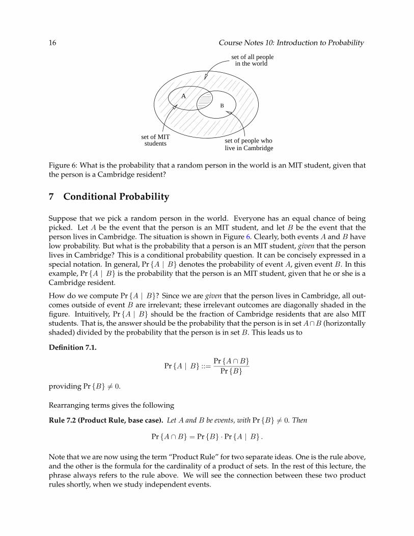
Figure 6: What is the probability that a random person in the world is an MIT student, given that the person is a Cambridge resident?
7 Conditional Probability
Suppose that we pick a random person in the world. Everyone has an equal chance of being picked. Let A be the event that the person is an MIT student, and let B be the event that the person lives in Cambridge. The situation is shown in Figure 6. Clearly, both events A and B have low probability. But what is the probability that a person is an MIT student, given that the person lives in Cambridge? This is a conditional probability question. It can be concisely expressed in a special notation. In general, Pr {A | B} denotes the probability of event A, given event B. In this example, Pr {A | B} is the probability that the person is an MIT student, given that he or she is a Cambridge resident.
How do we compute Pr {A | B}? Since we are given that the person lives in Cambridge, all out-comes outside of event B are irrelevant; these irrelevant outcomes are diagonally shaded in the figure. Intuitively, Pr {A | B} should be the fraction of Cambridge residents that are also MIT students. That is, the answer should be the probability that the person is in set A ∩ B (horizontally shaded) divided by the probability that the person is in set B. This leads us to
Definition 7.1.
Pr {A ∩ B}Pr {A | B} ::=
Pr {B}
providing Pr {B} �= 0.
Rearranging terms gives the following
Rule 7.2 (Product Rule, base case). Let A and B be events, with Pr {B} �= 0. Then
Pr {A ∩ B} = Pr {B} · Pr {A | B} .
Note that we are now using the term “Product Rule” for two separate ideas. One is the rule above, and the other is the formula for the cardinality of a product of sets. In the rest of this lecture, the phrase always refers to the rule above. We will see the connection between these two product rules shortly, when we study independent events.
Course Notes 10: Introduction to Probability 17
As an example, what is Pr {B | B}? That is, what is the probability of event B, given that event B happens? Intuitively, this ought to be 1! The Product Rule gives exactly this result if Pr {B} �= 0:
Pr {B ∩ B}Pr {B | B} =
Pr {B}
=Pr {B}Pr {B}
= 1
A routine induction proof based on the special case leads to The Product Rule for n events.
Rule 7.3 (Product Rule, general case). Let A1, A2, . . . , An be events.
Pr {A1 ∩ A2 ∩ · · · ∩ An} = Pr {A1} Pr {A2 | A1} Pr {A3 | A1 ∩ A2} · · · Pr {An | A1 ∩ · · · ∩ An−1}
7.1 Conditional Probability Identities
All our probability identities continue to hold when all probabilities are conditioned on the same event. For example,
Pr {A ∪ B | C} = Pr {A | C} + Pr {B | C} − Pr {A ∩ B | C} (Conditional Inclusion-Exclusion)
The identities carry over because for any event C, we can define a new probability measure, PrC {} on the same sample space by the rule that
PrC {A} ::= Pr {A | C} .
Now the conditional-probability version of an identity is just an instance of the original identity using the new probability measure.
Problem 1. Prove that for any probability space, S, and event C ⊆ S, the function PrC {} is a probability measure on S.
In carrying over identities to conditional versions, a common blunder is mixing up events before and after the conditioning bar. For example, the following is not a consequence of the Sum Rule:
False Claim 7.4.
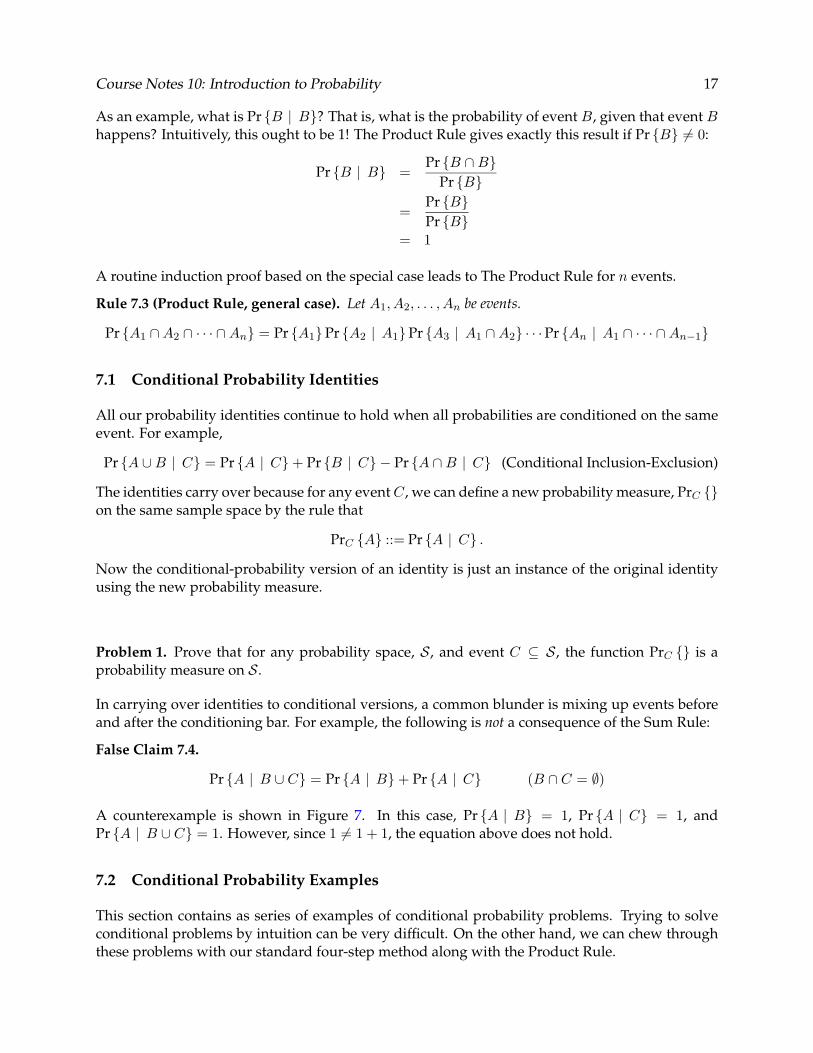
Pr {A | B ∪ C} = Pr {A | B} + Pr {A | C} (B ∩ C = ∅)
A counterexample is shown in Figure 7. In this case, Pr {A | B} = 1, Pr {A | C} = 1, and Pr {A | B ∪ C} = 1. However, since 1 �= 1 + 1, the equation above does not hold.
7.2 Conditional Probability Examples
This section contains as series of examples of conditional probability problems. Trying to solve conditional problems by intuition can be very difficult. On the other hand, we can chew through these problems with our standard four-step method along with the Product Rule.
18 Course Notes 10: Introduction to Probability
sample space
A
BC
Figure 7: This figure illustrates a case where the equation Pr {A | B ∪ C} = Pr {A | B} + Pr {A | C} does not hold.
7.2.1 A Two-out-of-Three Series
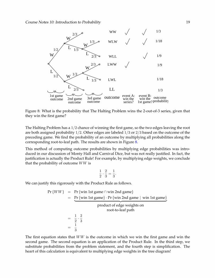
The MIT EECS department’s famed D-league hockey team, The Halting Problem, is playing a 2-out-of-3 series. That is, they play games until one team wins a total of two games. The probability that The Halting Problem wins the first game is 1/2. For subsequent games, the probability of winning depends on the outcome of the preceding game; the team is energized by victory and demoralized by defeat. Specifically, if The Halting Problem wins a game, then they have a 2/3 chance of winning the next game. On the other hand, if the team loses, then they have only a 1/3 chance of winning the following game. What is the probability that The Halting Problem wins the 2-out-of-3 series, given that they win the first game?
This problem involves two types of conditioning. First, we are told that the probability of the team winning a game is 2/3, given that they won the preceding game. Second, we are asked the odds of The Halting Problem winning the series, given that they win the first game.
Step 1: Find the Sample Space
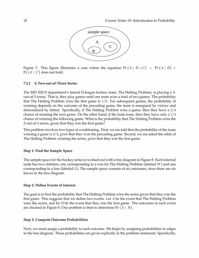
The sample space for the hockey series is worked out with a tree diagram in Figure 8. Each internal node has two children, one corresponding to a win for The Halting Problem (labeled W ) and one corresponding to a loss (labeled L). The sample space consists of six outcomes, since there are six leaves in the tree diagram.
Step 2: Define Events of Interest
The goal is to find the probability that The Halting Problem wins the series given that they win the first game. This suggests that we define two events. Let A be the event that The Halting Problem wins the series, and let B be the event that they win the first game. The outcomes in each event are checked in Figure 8. Our problem is then to determine Pr {A | B}.
Step 3: Compute Outcome Probabilities
Next, we must assign a probability to each outcome. We begin by assigning probabilities to edges in the tree diagram. These probabilities are given explicitly in the problem statement. Specifically,
� �� �
Course Notes 10: Introduction to Probability 19
2/3
L1/2
W1/2
W 1/3
L2/3
L 1/3
W2/3
LL 1/3
W2/3
W1/3
1st gameoutcome 2nd game
outcome3rd gameoutcome probability
outcome
1/3
1/18
1/9
1/9
1/18
1/3
event B:win the
1st game?
event A:win theseries?
WW
WLW
WLL
LWW
LWL
LL
outcome
Figure 8: What is the probability that The Halting Problem wins the 2-out-of-3 series, given that they win the first game?
The Halting Problem has a 1/2 chance of winning the first game, so the two edges leaving the root are both assigned probability 1/2. Other edges are labeled 1/3 or 2/3 based on the outcome of the preceding game. We find the probability of an outcome by multiplying all probabilities along the corresponding root-to-leaf path. The results are shown in Figure 8.
This method of computing outcome probabilities by multiplying edge probabilities was introduced in our discussion of Monty Hall and Carnival Dice, but was not really justified. In fact, the justification is actually the Product Rule! For example, by multiplying edge weights, we conclude that the probability of outcome WW is
1 2 1 =
2 · 3 3
.
We can justify this rigorously with the Product Rule as follows.
Pr {WW } = Pr {win 1st game ∩ win 2nd game}
= Pr {win 1st game} · Pr {win 2nd game | win 1st game}
product of edge weights on root-to-leaf path
1 2 =
2 · 3
1 =
3
The first equation states that WW is the outcome in which we win the first game and win the second game. The second equation is an application of the Product Rule. In the third step, we substitute probabilities from the problem statement, and the fourth step is simplification. The heart of this calculation is equivalent to multiplying edge weights in the tree diagram!
� �� �
20 Course Notes 10: Introduction to Probability
Here is a second example. By multiplying edge weights in the tree diagram, we conclude that the probability of outcome WLL is
1 1 2 1 =
2 · 3 · 3 9
.
We can formally justify this with the Product Rule as follows:
Pr {WLL} = Pr {win 1st ∩ lose 2nd ∩ lose 3rd}
= Pr {win 1st} · Pr {lose 2nd | win 1st} Pr {lose 3nd | win 1st ∩ lose 2nd}
product of edge weights on root-to-leaf path
1 1 2 =
2 · 3 · 3
1 =
9
Step 4: Compute Event Probabilities
We can now compute the probability that The Halting Problem wins the tournament given that they win the first game:
Pr {A | B} =
=
=
Pr {A ∩ B} Pr {B}
(Product Rule)
1/3 + 1/18 1/3 + 1/18 + 1/9
(Sum Rule for Pr {B})
7 9 .
The Halting Problem has a 7/9 chance of winning the tournament, given that they win the first game.
7.2.2 An a posteriori Probability
In the preceding example, we wanted the probability of an event A, given an earlier event B. In particular, we wanted the probability that The Halting Problem won the series, given that they won the first game. It can be harder to think about the probability of an event A, given a later event B. For example, what is the probability that The Halting Problem wins its first game, given that the team wins the series? This is called an a posteriori probability.
An a posteriori probability question can be interpreted in two ways. By one interpretation, we reason that since we are given the series outcome, the first game is already either won or lost; we do not know which. The issue of who won the first game is a question of fact, not a question of probability. Though this interpretation may have philosophical merit, we will never use it.
We will always prefer a second interpretation. Namely, we suppose that the experiment is run over and over and ask in what fraction of the experiments did event A occur when event B occurred?
Course Notes 10: Introduction to Probability 21
For example, if we run many hockey series, in what fraction of the series did the Halting Problem win the first game when they won the whole series? Under this interpretation, whether A precedes B in time is irrelevant. In fact, we will solve a posteriori problems exactly the same way as other conditional probability problems. The only trick is to avoid being confused by the wording of the problem!
We can now compute the probability that The Halting Problem wins its first game, given that the team wins the series. The sample space is unchanged; see Figure 8. As before, let A be the event that The Halting Problem wins the series, and let B be the event that they win the first game. We already computed the probability of each outcome; all that remains is to compute the probability of event Pr {B | A}:
Pr {B ∩ A}Pr {B | A} =
Pr {A} 1/3 + 1/18
1/3 + 1/18 + 1/9=
79
=
The probability of The Halting Problem winning the first game, given that they won the series is 7/9.
This answer is suspicious! In the preceding section, we showed that Pr {A | B} = 7/9. Could it be true that Pr {A | B} = Pr {B | A} in general? We can determine the conditions under which this equality holds by writing Pr {A ∩ B} = Pr {B ∩ A} in two different ways as follows:
Pr {A | B} Pr {B} = Pr {A ∩ B} = Pr {B ∩ A} = Pr {B | A} Pr {A} .
Evidently, Pr {A | B} = Pr {B | A} only when Pr {A} = Pr {B} �= 0. This is true for the hockey problem, but only by coincidence. In general, Pr {A | B} and Pr {B | A} are not equal!
7.2.3 A Problem with Two Coins [Optional]
[Optional]
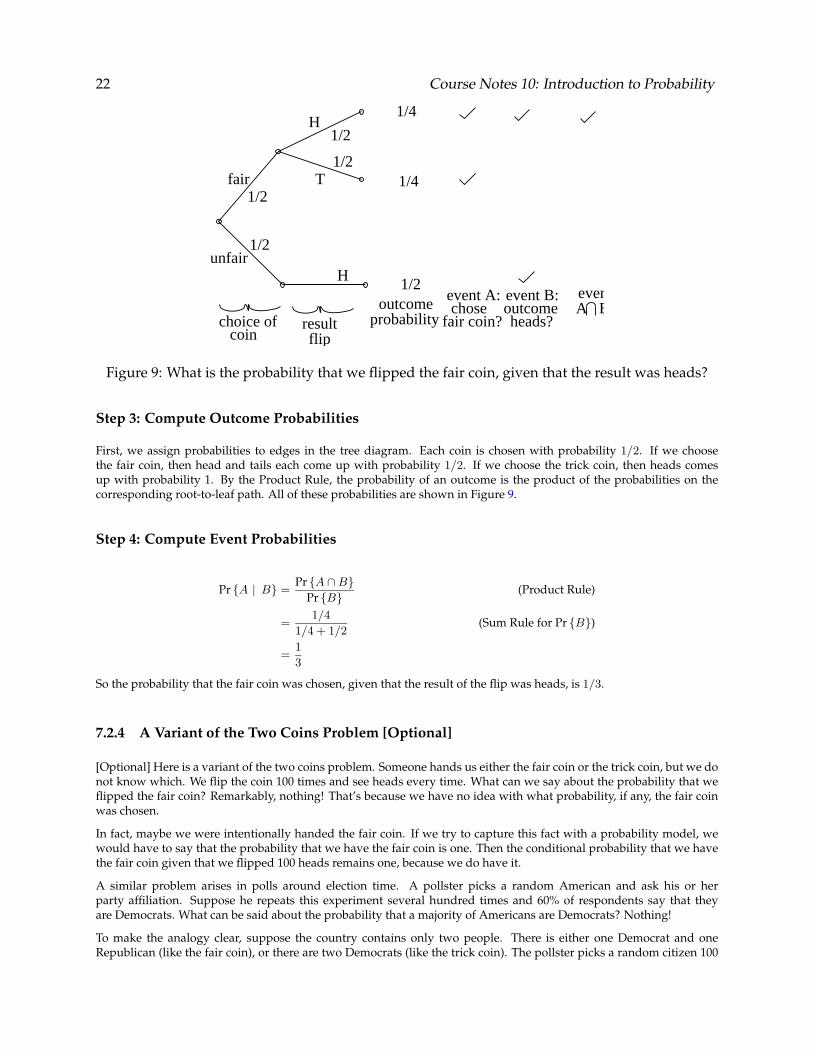
We have two coins. One coin is fair; that is, comes up heads with probability 1/2 and tails with probability 1/2. The other is a trick coin; it has heads on both sides, and so always comes up heads. Now suppose we randomly choose one of the coins, without knowing one we’re picking and with each coin equally likely. If we flip this coin and get heads, then what is the probability that we flipped the fair coin?
This is one of those tricky a posteriori problems, since we want the probability of an event (the fair coin was chosen) given the outcome of a later event (heads came up). Intuition may fail us, but the standard four-step method works perfectly well.
Step 1: Find the Sample Space
The sample space is worked out with the tree diagram in Figure 9.
Step 2: Define Events of Interest
Let A be the event that the fair coin was chosen. Let B the event that the result of the flip was heads. The outcomes in each event are marked in the figure. We want to compute Pr {A | B}, the probability that the fair coin was chosen, given that the result of the flip was heads.
22 Course Notes 10: Introduction to Probability
fair
unfair
choice ofcoin
result
H
flip
1/2
1/2
1/2
1/2
H
T
1/2
1/4
1/4
event A:outcomeprobability fair coin?
event B:outcomeheads?
eventchose A B?
Figure 9: What is the probability that we flipped the fair coin, given that the result was heads?
Step 3: Compute Outcome Probabilities
First, we assign probabilities to edges in the tree diagram. Each coin is chosen with probability 1/2. If we choose the fair coin, then head and tails each come up with probability 1/2. If we choose the trick coin, then heads comes up with probability 1. By the Product Rule, the probability of an outcome is the product of the probabilities on the corresponding root-to-leaf path. All of these probabilities are shown in Figure 9.
Step 4: Compute Event Probabilities
Pr {A | B} = Pr {A ∩ B}
(Product Rule)Pr {B}1/4
=1/4 + 1/2
(Sum Rule for Pr {B})
1 =
3
So the probability that the fair coin was chosen, given that the result of the flip was heads, is 1/3.
7.2.4 A Variant of the Two Coins Problem [Optional]
[Optional] Here is a variant of the two coins problem. Someone hands us either the fair coin or the trick coin, but we do not know which. We flip the coin 100 times and see heads every time. What can we say about the probability that we flipped the fair coin? Remarkably, nothing! That’s because we have no idea with what probability, if any, the fair coin was chosen.
In fact, maybe we were intentionally handed the fair coin. If we try to capture this fact with a probability model, we would have to say that the probability that we have the fair coin is one. Then the conditional probability that we have the fair coin given that we flipped 100 heads remains one, because we do have it.
A similar problem arises in polls around election time. A pollster picks a random American and ask his or her party affiliation. Suppose he repeats this experiment several hundred times and 60% of respondents say that they are Democrats. What can be said about the probability that a majority of Americans are Democrats? Nothing!
To make the analogy clear, suppose the country contains only two people. There is either one Democrat and one Republican (like the fair coin), or there are two Democrats (like the trick coin). The pollster picks a random citizen 100
Course Notes 10: Introduction to Probability 23
times; this is analogous to flipping the coin 100 times. Even if he always picks a Democrat (flips heads), he can not determine the probability that the country is all Democrat!
Of course, if we have the fair coin, it is very unlikely that we would flip 100 heads. So in practice, if we got 100 heads, we would bet with confidence that we did not have the fair coin. This distinction between the probability of an event— which may be undefined—and the confidence we may have in its occurrence is central to statistical reasoning about real data. We’ll return to this important issue in the coming weeks.
7.2.5 Medical Testing
There is a degenerative disease called Zostritis that 10% of men in a certain population may suffer in old age. However, if treatments are started before symptoms appear, the degenerative effects can largely be controlled.
Fortunately, there is a test that can detect latent Zostritis before any degenerative symptoms appear. The test is not perfect, however:
• If a man has latent Zostritis, there is a 10% chance that the test will say he does not. (These are called “false negatives”.)
• If a man does not have latent Zostritis, there is a 30% chance that the test will say he does. (These are “false positives”.)
A random man is tested for latent Zostritis. If the test is positive, then what is the probability that the man has latent Zostritis?
Step 1: Find the Sample Space
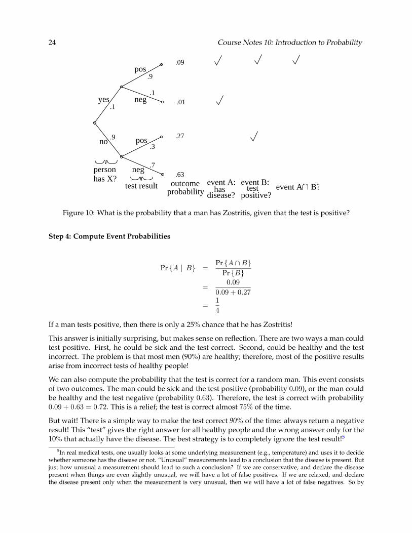
The sample space is found with a tree diagram in Figure 10.
Step 2: Define Events of Interest
Let A be the event that the man has Zostritis. Let B be the event that the test was positive. The outcomes in each event are marked in Figure 10. We want to find Pr {A | B}, the probability that a man has Zostritis, given that the test was positive.
Step 3: Find Outcome Probabilities
First, we assign probabilities to edges. These probabilities are drawn directly from the problem statement. By the Product Rule, the probability of an outcome is the product of the probabilities on the corresponding root-to-leaf path. All probabilities are shown in the figure.
24 Course Notes 10: Introduction to Probability
personhas X?
test result outcomeprobability event A B?
yes
no
pos
neg
pos
neg
.1
.9
.9
.1
.3
.7
.09
.01
.27
.63event A: event B:
hasdisease?
testpositive?
Figure 10: What is the probability that a man has Zostritis, given that the test is positive?
Step 4: Compute Event Probabilities
Pr {A | B} = Pr {A ∩ B}
Pr {B}0.09
= 0.09 + 0.27 1
= 4
If a man tests positive, then there is only a 25% chance that he has Zostritis!
This answer is initially surprising, but makes sense on reflection. There are two ways a man could test positive. First, he could be sick and the test correct. Second, could be healthy and the test incorrect. The problem is that most men (90%) are healthy; therefore, most of the positive results arise from incorrect tests of healthy people!
We can also compute the probability that the test is correct for a random man. This event consists of two outcomes. The man could be sick and the test positive (probability 0.09), or the man could be healthy and the test negative (probability 0.63). Therefore, the test is correct with probability 0.09 + 0.63 = 0.72. This is a relief; the test is correct almost 75% of the time.
But wait! There is a simple way to make the test correct 90% of the time: always return a negative result! This “test” gives the right answer for all healthy people and the wrong answer only for the 10% that actually have the disease. The best strategy is to completely ignore the test result!5
5In real medical tests, one usually looks at some underlying measurement (e.g., temperature) and uses it to decide whether someone has the disease or not. “Unusual” measurements lead to a conclusion that the disease is present. But just how unusual a measurement should lead to such a conclusion? If we are conservative, and declare the disease present when things are even slightly unusual, we will have a lot of false positives. If we are relaxed, and declare the disease present only when the measurement is very unusual, then we will have a lot of false negatives. So by
� �
� � �
� � � � � � �
� � �
Course Notes 10: Introduction to Probability 25
There is a similar paradox in weather forecasting. During winter, almost all days in Boston are wet and overcast. Predicting miserable weather every day may be more accurate than really trying to get it right! This phenomenon is the source of many paradoxes; we will see more in coming weeks.
7.3 Confusion about Monty Hall
Using conditional probability we can examine the main argument that confuses people about the Monty Hall example of Section 3.
Let the doors be numbered 1, 2, 3, and suppose the contestant chooses door 1 and then Carol opens door 2. Now the contestant has to decide whether to stick with door 1 or switch to door 3. To do this, he considers the probability that the prize is behind the remaining unopened door 3, given that he has learned that it is not behind door 2.
To calculate this conditional probability, let W be the event that the contestant chooses door 1, and let Ri be the event that the prize is behind door i, for i = 1, 2, 3. The contestant knows that Pr {W } = 1/3 = Pr {Ri}, and since his choice has no efffect on the location of the prize, he can say that
1 1 1Pr {Ri ∩ W } = Pr {Ri} · Pr {W } =
3 · 3
=9
and likewise,
Pr Ri ∩ W = (2/3)(1/3) = 2/9,
for i = 1, 2, 3.
Now the probability that the prize is behind the remaining unopened door 3, given that the contestant has learned that it is not behind door 2 is Pr R3 ∩ W � R2 ∩ W . But
Pr R3 ∩ W � R2 ∩ W ::= Pr R �3 ∩ R2 ∩ W
= Pr {R3} ∩ W � =
1/9=
1
Pr R2 ∩ W Pr R2 ∩ W 2/9 2 .
Likewise, Pr R1 ∩ W � R2 ∩ W = 1/2. So the contestant concludes that the prize is equally likely to be behind door 1 as behind door 3, and therefore there is no advantage to the switch strategy over the stick strategy. But this contradicts our earlier analysis!
Whew, that is confusing! Where did the contestant’s reasoning go wrong? (Maybe, like some Ph.D. mathematicians, you are convinced by the contestant’s reasoning and now think we must have made a mistake in our earlier conclusion that switching is twice as likely to win than sticking.) Let’s try to sort this out.
There is a fallacy in the contestant’s reasoning—a subtle one. In fact, his calculation that, given that the prize is not behind door 2, that it’s equally likely to be behind door 1 as door 3 is correct. His mistake is in not realizing that he knows more than that the prize is not behind door 2. He has confused two similar, but distinct, events, namely,
shifting the decision threshold, one can trade off on false positives versus false negatives. It appears that the tester in our example above did not choose the right threshold for their test—they can probably get higher overall accuracy by allowing a few more false negatives to get fewer false positives.
26 Course Notes 10: Introduction to Probability
1. the contestant chooses door 1 and the prize is not behind door 2, and,
2. the contestant chooses door 1 and then Carol opens door 2..
These are different events and indeed they have different probabilities. The fact that Carol opens door 2 tells the contestant more than that the prize is not behind door 2.
We can precisely demonstrate this with our sample space of triples (i, j, k), where the prize is behind door i, the contestant picks door j, and Carol opens door k. In particular, let Ci be the event that Carol opens door i. Then, event 1. is R2 ∩ W , and event 2. is W ∩ C2.
We can confirm the correctness of the contestant’s calculation that the prize is behind door 1 given event 1:
R2 ∩ W ::= {(1, 1, 2), (3, 1, 2), (1, 1, 3)}� � 1 1 1 2Pr R2 ∩ W = =
18+
9+
18=
9
Pr � R1 �� R2 ∩ W
� =
Pr {{(1, 1, 2), (1, 1, 3)}} 1 =
2/9 2 .
But although the contestant’s calculation is correct, his blunder is that he calculated the wrong thing. Specifically, he conditioned his conclusion on the wrong event. The contestant’s situation when he must decide to stick or switch is that event 2. has occurred. So he should have calculated:
W ∩ C2 ::= {(1, 1, 2), (3, 1, 2)}1 1 1
Pr {W ∩ C2} = 18
+9
=6
Pr {R1 | W ∩ C2} = Pr {(1, 1, 2)}
=1
1/6 3 .
In other words, the probability that the prize is behind his chosen door 1 is 1/3, so he should switch because the probability is 2/3 that the prize is behind the other door 3, exactly as we correctly concluded in Section 3.
Once again, we see that mistaken intuition gets resolved by falling back on an examination of outcomes in the probability space.
8 Case Analysis
Combining the sum and product rules provides a natural way to determine the probabilities of complex events via case analysis. As a motivating example, we consider a rather paradoxical true story.
8.1 Discrimination Lawsuit
Several years ago there was a sex discrimination lawsuit against Berkeley. A female professor was denied tenure, allegedly because she was a woman. She argued that in every one of Berkeley’s 22 departments, the percentage of male applicants accepted was greater than the percentage of female applicants accepted. This sounds very suspicious, if not paradoxical!
Course Notes 10: Introduction to Probability 27
However, Berkeley’s lawyers argued that across the whole university the percentage of male applicants accepted was actually lower than the percentage of female applicants accepted! This suggests that if there was any sex discrimination, then it was against men! Must one party in the dispute be lying?
8.1.1 A false analysis
Here is a fallacious analysis of the discrimination lawsuit.
To clarify the arguments, let’s and express them in terms of conditional probabilities. Suppose that there are only two departments, EE and CS, and consider the experiment where we ignore gender and pick an applicant at random. Define the following events:
• Let A be the event that the applicant is accepted.
• Let FEE the event that the applicant is a female applying to EE.
• Let FCS the event that the applicant is a female applying to CS.
• Let MEE the event that the applicant is a male applying to EE.
• Let MCS the event that the applicant is a male applying to CS.
Assume that all applicants are either male or female, and that no applicant applied to both departments. That is, the events FEE , FCS , MEE , and MCS are all disjoint.
The female plaintiff makes the following argument:
Pr {A | FEE } < Pr {A | MEE } (7) Pr {A | FCS } < Pr {A | MCS } (8)
That is, in both departments, the probability that a woman is accepted is less than the probability that a man is accepted. The university retorts that overall a woman applicant is more likely to be accepted than a man:
Pr {A | FEE ∪ FCS } > Pr {A | MEE ∪ MCS } (9)
It is easy to believe that these two positions are contradictory.
[Optional] In fact, we might even try to prove this as follows:
Pr {A | FEE } + Pr {A | FCS } < Pr {A | MEE } + Pr {A | MCS } (by (7) & (8)). (10)
Therefore
Pr {A | FEE ∪ FCS } < Pr {A | MEE ∪ MCS } , (11)
which exactly contradicts the university’s position!
However, there is a problem with this argument; equation (11) follows (10) only if we accept False Claim 7.4 above! Therefore, this argument is invalid.
�
�
28 Course Notes 10: Introduction to Probability
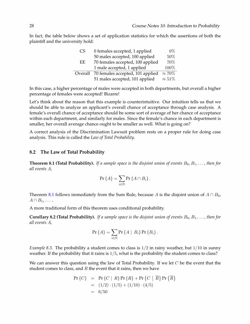
In fact, the table below shows a set of application statistics for which the assertions of both theplaintiff and the university hold:
CS 0 females accepted, 1 applied 0% 50 males accepted, 100 applied 50%
EE 70 females accepted, 100 applied 70% 1 male accepted, 1 applied 100%
Overall 70 females accepted, 101 applied ≈ 70% 51 males accepted, 101 applied ≈ 51%
In this case, a higher percentage of males were accepted in both departments, but overall a higher percentage of females were accepted! Bizarre!
Let’s think about the reason that this example is counterintuitive. Our intuition tells us that we should be able to analyze an applicant’s overall chance of acceptance through case analysis. A female’s overall chance of acceptance should be some sort of average of her chance of acceptance within each department, and similarly for males. Since the female’s chance in each department is smaller, her overall average chance ought to be smaller as well. What is going on?
A correct analysis of the Discrimination Lawsuit problem rests on a proper rule for doing case analysis. This rule is called the Law of Total Probability.
8.2 The Law of Total Probability
Theorem 8.1 (Total Probability). If a sample space is the disjoint union of events B0, B1, . . . , then for all events A,
Pr {A} = Pr {A ∩ Bi} . i∈N
Theorem 8.1 follows immediately from the Sum Rule, because A is the disjoint union of A ∩ B0, A ∩ B1, . . . .
A more traditional form of this theorem uses conditional probability.
Corollary 8.2 (Total Probability). If a sample space is the disjoint union of events B0, B1, . . . , then for all events A,
Pr {A} = Pr {A | Bi} Pr {Bi} . i∈N
Example 8.3. The probability a student comes to class is 1/2 in rainy weather, but 1/10 in sunny weather. If the probability that it rains is 1/5, what is the probability the student comes to class?
We can answer this question using the law of Total Probability. If we let C be the event that the student comes to class, and R the event that it rains, then we have � � � � �
Pr {C} = Pr {C | R} Pr {R} + Pr C � R Pr R
= (1/2) · (1/5) + (1/10) · (4/5) = 6/50
Course Notes 10: Introduction to Probability 29
8.3 Resolving the Discrimination Lawsuit Paradox
With the law of total probability in hand, we can perform a proper case analysis for our discrimination lawsuit.
Let FA be the event that a female applicant is accepted.
Assume that no applicant applied to both departments. That is, the events, FEE , that the female applicant is applying to EE, and FCS , that she is applying to CS, are disjoint (and in fact complementary).
Since FEE and FCS partition the sample space, we can apply the law of total probability to analyze acceptance probability:
Pr {FA} = Pr {FA | FEE } Pr {FEE } + Pr {FA | FCS } Pr {FCS }
= (70/100) · (100/101) + (0/1) · (1/101) = 70/101,
which is the correct answer. Notice that as we intuited, Pr {FA} is a weighted average of the conditional probabilities of FA, where the weights (of 100/101 and 1/101 respectively) are simply the probabilities of being in each condition.
In the same fashion, we can define the events MA and evaluate a male’s overall acceptance probability:
Pr {MA} = Pr {MA | MEE } Pr {MEE } + Pr {MA | MCS } Pr {MCS }
= (1/1) · (1/101) + (50/100) · (100/101) = 51/101,
which is the correct answer. As before, the overall acceptance probability is a weighted average of the conditional acceptance probabilities.
But here we have the source of our paradox: the weights of the weighted averages for males and females are different. For the females, the bulk of the weight (common department) falls on the condition (department) in which females do very well (EE); thus the weighted average for females is quite good. For the males, the bulk of the weight falls on the condition in which males do poorly (CS); thus the weighted average for males is poor.
Which brings us back to the allegation in the lawsuit. Having precisely analyzed the arguments of the plaintiff and the defendent, you are in a position to judge how persuasive they are. If you were on the jury, would you find Berkeley guilty of gender bias in its admissions?
8.4 On-Time Airlines
[Optional]
Here is a second example of the same paradox. Newspapers publish on-time statistics for airlines to help travelers choose the best carrier. The on-time rate for an airline is defined as follows:
Airline on-time rate = #flights less than 15 minutes late
#flights total
� W
� �
� W
� � � F
�
30 Course Notes 10: Introduction to Probability
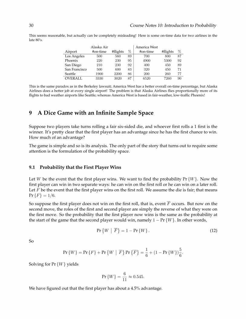
This seems reasonable, but actually can be completely misleading! Here is some on-time data for two airlines in the late 80’s.
Alaska Air America West Airport #on-time #flights % #on-time #flights % Los Angeles 500 560 89 700 800 87 Phoenix 220 230 95 4900 5300 92 San Diego 210 230 92 400 450 89 San Francisco 500 600 83 320 450 71 Seattle 1900 2200 86 200 260 77 OVERALL 3330 3020 87 6520 7260 90
This is the same paradox as in the Berkeley lawsuit; America West has a better overall on-time percentage, but Alaska Airlines does a better job at every single airport! The problem is that Alaska Airlines flies proportionally more of its flights to bad weather airports like Seattle; whereas America West is based in fair-weather, low-traffic Phoenix!
9 A Dice Game with an Infinite Sample Space
Suppose two players take turns rolling a fair six-sided die, and whoever first rolls a 1 first is the winner. It’s pretty clear that the first player has an advantage since he has the first chance to win. How much of an advantage?
The game is simple and so is its analysis. The only part of the story that turns out to require some attention is the formulation of the probability space.
9.1 Probability that the First Player Wins
Let W be the event that the first player wins. We want to find the probability Pr {W }. Now the first player can win in two separate ways: he can win on the first roll or he can win on a later roll. Let F be the event that the first player wins on the first roll. We assume the die is fair; that means Pr {F } = 1/6.
So suppose the first player does not win on the first roll, that is, event F occurs. But now on the second move, the roles of the first and second player are simply the reverse of what they were on the first move. So the probability that the first player now wins is the same as the probability at the start of the game that the second player would win, namely 1 − Pr {W }. In other words,
� F = 1 − Pr {W } . (12)Pr
So
� F Pr =1 6
+ (1 − Pr {W })5 6 .Pr {W } = Pr {F } + Pr
Solving for Pr {W } yields
6Pr {W } =
11 ≈ 0.545.
We have figured out that the first player has about a 4.5% advantage.
�
Course Notes 10: Introduction to Probability 31
9.2 The Possibility of a Tie
Our calculation that Pr {W } = 6/11 is correct, but it rests on an important, hidden assumption. We assumed that the second player does win if the first player does not win. In other words, there will always be a winner. This seems obvious until we realize that there may be a game in which neither player wins—the players might roll forever without rolling a 1. Our assumption is wrong!
But a more careful look at the reasoning above reveals that we didn’t actually assume that there always is a winner. All we need to justify is the assumption that the probability that the second player wins equals one minus the probability that the first player wins. This is equivalent to assuming, not that there will always be a winner, but only that the probability is 1 that there is a winner.
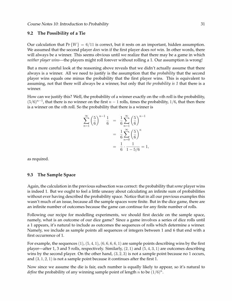
How can we justify this? Well, the probability of a winner exactly on the nth roll is the probability, (5/6)n−1 , that there is no winner on the first n − 1 rolls, times the probability, 1/6, that then there is a winner on the nth roll. So the probability that there is a winner is
� � 5 �n−1 1 1 � �
5 �n−1∞ ∞
= 6 6 6 6
n=1 n=1 ∞
n=0
�5 6
�n16
=
16· 1
= 1,1 − 5/6
=
as required.
9.3 The Sample Space
Again, the calculation in the previous subsection was correct: the probability that some player wins is indeed 1. But we ought to feel a little uneasy about calculating an infinite sum of probabilities without ever having described the probability space. Notice that in all our previous examples this wasn’t much of an issue, because all the sample spaces were finite. But in the dice game, there are an infinite number of outcomes because the game can continue for any finite number of rolls.
Following our recipe for modelling experiments, we should first decide on the sample space, namely, what is an outcome of our dice game? Since a game involves a series of dice rolls until a 1 appears, it’s natural to include as outcomes the sequences of rolls which determine a winner. Namely, we include as sample points all sequences of integers between 1 and 6 that end with a first occurrence of 1.
For example, the sequences (1), (5, 4, 1), (6, 6, 6, 6, 1) are sample points describing wins by the first player—after 1, 3 and 5 rolls, respectively. Similarly, (2, 1) and (5, 4, 3, 1) are outcomes describing wins by the second player. On the other hand, (3, 2, 3) is not a sample point because no 1 occurs, and (3, 1, 2, 1) is not a sample point because it continues after the first 1.
Now since we assume the die is fair, each number is equally likely to appear, so it’s natural to define the probability of any winning sample point of length n to be (1/6)n .
32 Course Notes 10: Introduction to Probability
The outcomes in the event that there is a winner on the nth roll are the 5n−1 length-n sequences whose first 1 occurs in the nth position. Therefore this event has the probability
� 1 �n �
5 �n−1 1
5n−1 = 6 6 6
.
This is the probability that we used in the previous subsection to calculate that the probability is 1 that there is a winner.
Besides winning sequences, which are necessarily of finite length, we should consider including sample points corresponding to games with no winner. Now since the winning probabilities already total to one, any sample points we choose to reflect no-winner situations must be assigned probability zero, and moreover the event consisting of all the no-winner points that we include must have probability zero.
A natural choice for the no-winner outcomes would be all the infinite sequences of integers be-tween 2 and 6, namely, those with no occurrence of a 1. This leads to a legitimate sample space. But for the analysis we just did of the dice game, it makes absolutely no difference what no-win out- comes we include. In fact, it doesn’t matter whether we include any no-win points at all.
It does seem a little strange to model the game in a way that denies the logical possibility of an infinite sequence of rolls. On the other hand, we have no need to model the details of the infinite sequences of rolls when there is no winner. So let’s define our sample space to include a single additional outcome which does represent the possibility of the game continuing forever with no winner; the probability of this “no winner” point is defined to be 0. So this choice of sample space acknowledges the logical possibility of an infinite game.6
10 Independence
10.1 The Definition
Definition 10.1. Suppose A and B are events, and B has positive probability. Then A is indepen- dent of B iff
Pr {A | B} = Pr {A} .
In other words, that fact that event B occurs does not affect the probability that event A occurs.
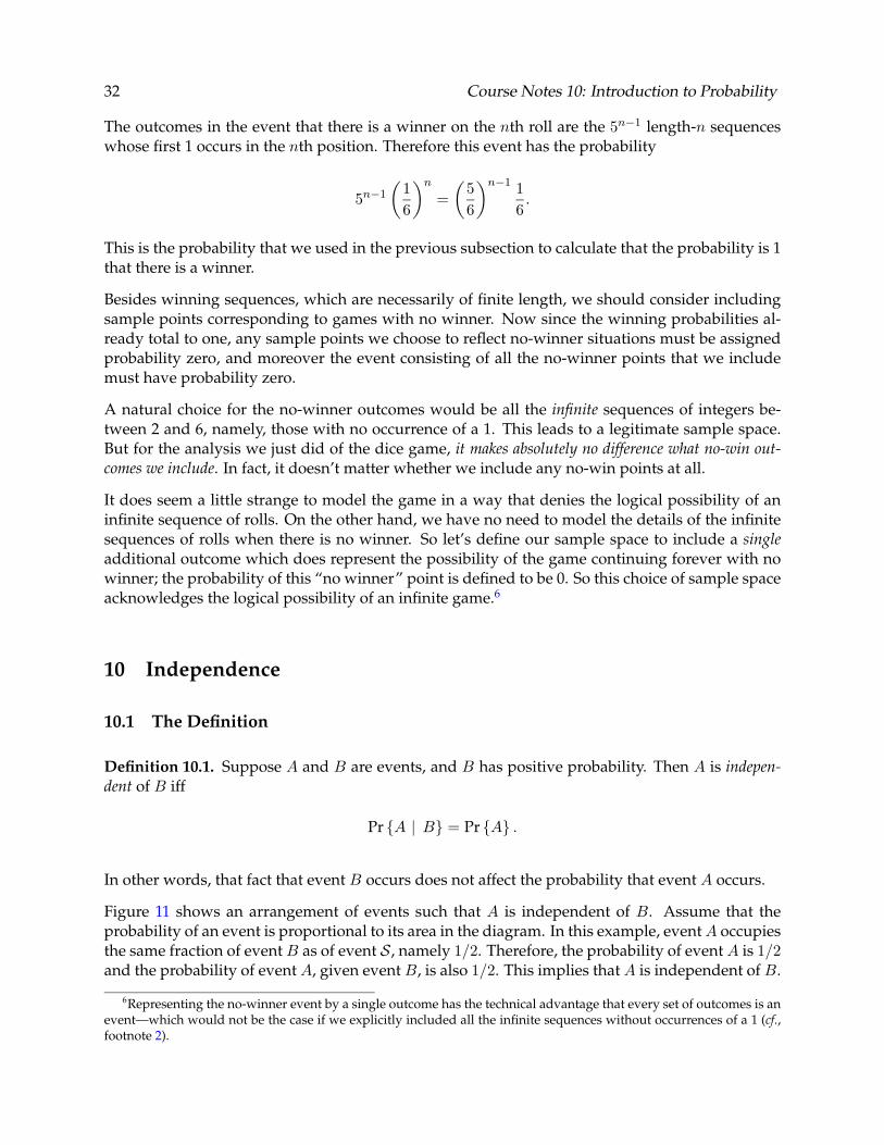
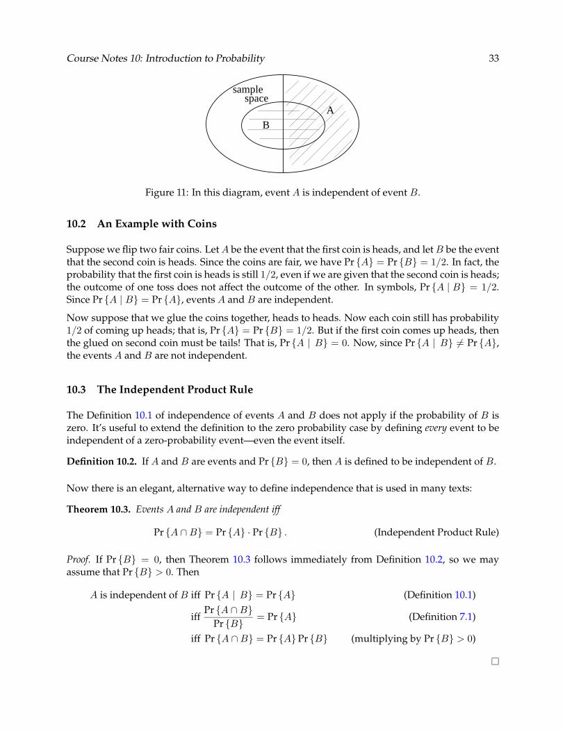
Figure 11 shows an arrangement of events such that A is independent of B. Assume that the probability of an event is proportional to its area in the diagram. In this example, event A occupies the same fraction of event B as of event S, namely 1/2. Therefore, the probability of event A is 1/2 and the probability of event A, given event B, is also 1/2. This implies that A is independent of B.
6Representing the no-winner event by a single outcome has the technical advantage that every set of outcomes is an event—which would not be the case if we explicitly included all the infinite sequences without occurrences of a 1 (cf., footnote 2).
Course Notes 10: Introduction to Probability 33
samplespace
BA
Figure 11: In this diagram, event A is independent of event B.
10.2 An Example with Coins
Suppose we flip two fair coins. Let A be the event that the first coin is heads, and let B be the event that the second coin is heads. Since the coins are fair, we have Pr {A} = Pr {B} = 1/2. In fact, the probability that the first coin is heads is still 1/2, even if we are given that the second coin is heads; the outcome of one toss does not affect the outcome of the other. In symbols, Pr {A | B} = 1/2. Since Pr {A | B} = Pr {A}, events A and B are independent.
Now suppose that we glue the coins together, heads to heads. Now each coin still has probability 1/2 of coming up heads; that is, Pr {A} = Pr {B} = 1/2. But if the first coin comes up heads, then the glued on second coin must be tails! That is, Pr {A | B} = 0. Now, since Pr {A | B} �= Pr {A}, the events A and B are not independent.
10.3 The Independent Product Rule
The Definition 10.1 of independence of events A and B does not apply if the probability of B is zero. It’s useful to extend the definition to the zero probability case by defining every event to be independent of a zero-probability event—even the event itself.
Definition 10.2. If A and B are events and Pr {B} = 0, then A is defined to be independent of B.
Now there is an elegant, alternative way to define independence that is used in many texts:
Theorem 10.3. Events A and B are independent iff
Pr {A ∩ B} = Pr {A} · Pr {B} . (Independent Product Rule)
Proof. If Pr {B} = 0, then Theorem 10.3 follows immediately from Definition 10.2, so we may assume that Pr {B} > 0. Then
A is independent of B iff Pr {A | B} = Pr {A} (Definition 10.1)
iff Pr {A ∩ B}
= Pr {A} (Definition 7.1)Pr {B}
iff Pr {A ∩ B} = Pr {A} Pr {B} (multiplying by Pr {B} > 0)
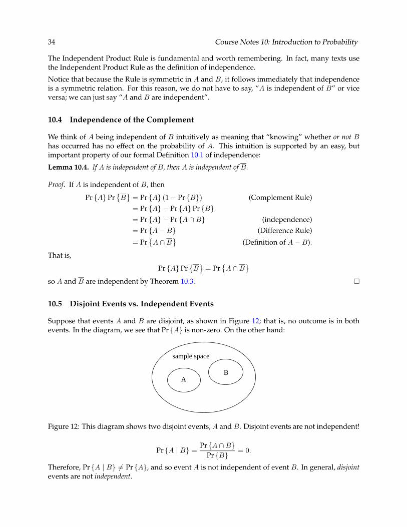
� �
� �
� � � �
34 Course Notes 10: Introduction to Probability
The Independent Product Rule is fundamental and worth remembering. In fact, many texts use the Independent Product Rule as the definition of independence.
Notice that because the Rule is symmetric in A and B, it follows immediately that independence is a symmetric relation. For this reason, we do not have to say, “A is independent of B” or vice versa; we can just say “A and B are independent”.
10.4 Independence of the Complement
We think of A being independent of B intuitively as meaning that “knowing” whether or not B has occurred has no effect on the probability of A. This intuition is supported by an easy, but important property of our formal Definition 10.1 of independence:
Lemma 10.4. If A is independent of B, then A is independent of B.
Proof. If A is independent of B, then
Pr {A} Pr B = Pr {A} (1 − Pr {B}) (Complement Rule) = Pr {A} − Pr {A} Pr {B}
= Pr {A} − Pr {A ∩ B} (independence) = Pr {A − B} (Difference Rule)
= Pr A ∩ B (Definition of A − B).
That is,
Pr {A} Pr B = Pr A ∩ B
so A and B are independent by Theorem 10.3.
10.5 Disjoint Events vs. Independent Events
Suppose that events A and B are disjoint, as shown in Figure 12; that is, no outcome is in both events. In the diagram, we see that Pr {A} is non-zero. On the other hand:
AB
sample space
Figure 12: This diagram shows two disjoint events, A and B. Disjoint events are not independent!
Pr {A | B} = Pr {A ∩ B}
= 0.Pr {B}
Therefore, Pr {A | B} �= Pr {A}, and so event A is not independent of event B. In general, disjoint events are not independent.
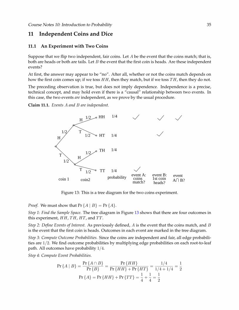
Course Notes 10: Introduction to Probability 35
11 Independent Coins and Dice
11.1 An Experiment with Two Coins
Suppose that we flip two independent, fair coins. Let A be the event that the coins match; that is, both are heads or both are tails. Let B the event that the first coin is heads. Are these independent events?
At first, the answer may appear to be “no”. After all, whether or not the coins match depends on how the first coin comes up; if we toss HH , then they match, but if we toss TH , then they do not.
The preceding observation is true, but does not imply dependence. Independence is a precise, technical concept, and may hold even if there is a “causal” relationship between two events. In this case, the two events are independent, as we prove by the usual procedure.
Claim 11.1. Events A and B are independent.
T
H
H
H
T
T1/2
1/2
1/2
1/2
1/2
1/2
TT
TH
HT
HH
probabilitycoin2coin 1event A:coinsmatch?
event B:1st coinheads?
1/4
1/4
1/4
1/4eventA B?
Figure 13: This is a tree diagram for the two coins experiment.
Proof. We must show that Pr {A | B} = Pr {A}.
Step 1: Find the Sample Space. The tree diagram in Figure 13 shows that there are four outcomes in this experiment, HH , TH , HT , and TT .
Step 2: Define Events of Interest. As previously defined, A is the event that the coins match, and B is the event that the first coin is heads. Outcomes in each event are marked in the tree diagram.
Step 3: Compute Outcome Probabilities. Since the coins are independent and fair, all edge probabilities are 1/2. We find outcome probabilities by multiplying edge probabilities on each root-to-leaf path. All outcomes have probability 1/4.
Step 4: Compute Event Probabilities.
Pr {HH} 1/4 1Pr {A | B} =
Pr {A ∩ B} =
Pr {HH } + Pr {HT } =
1/4 + 1/4=
2Pr {B} 1 1 1
Pr {A} = Pr {HH} + Pr {TT } =4
+4
=2
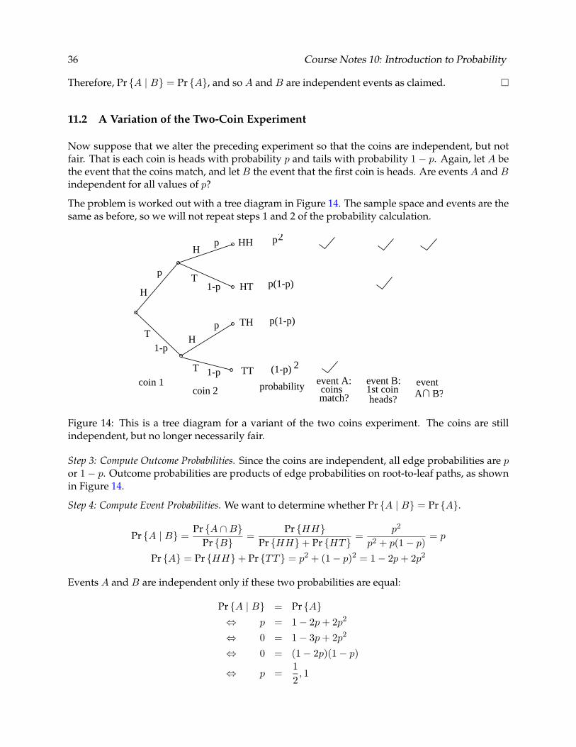
36 Course Notes 10: Introduction to Probability
Therefore, Pr {A | B} = Pr {A}, and so A and B are independent events as claimed.
11.2 A Variation of the Two-Coin Experiment
Now suppose that we alter the preceding experiment so that the coins are independent, but not fair. That is each coin is heads with probability p and tails with probability 1 − p. Again, let A be the event that the coins match, and let B the event that the first coin is heads. Are events A and B independent for all values of p?
The problem is worked out with a tree diagram in Figure 14. The sample space and events are the same as before, so we will not repeat steps 1 and 2 of the probability calculation.
T
H
H
H
T
T
TT
TH
HT
HH
probability event A:coinsmatch?
event B:1st coinheads?
eventA B?
p
p
p
1-p
1-p
1-p
(1-p) 2
p(1-p)
p(1-p)
p2
coin 2coin 1
Figure 14: This is a tree diagram for a variant of the two coins experiment. The coins are still independent, but no longer necessarily fair.
Step 3: Compute Outcome Probabilities. Since the coins are independent, all edge probabilities are p or 1 − p. Outcome probabilities are products of edge probabilities on root-to-leaf paths, as shown in Figure 14.
Step 4: Compute Event Probabilities. We want to determine whether Pr {A | B} = Pr {A}.
Pr {HH} p2
Pr {A | B} = Pr {A ∩ B}
= Pr {HH} + Pr {HT }
= p2 + p(1 − p)
= pPr {B}
Pr {A} = Pr {HH} + Pr {TT } = p2 + (1 − p)2 = 1 − 2p + 2p2
Events A and B are independent only if these two probabilities are equal:
Pr {A | B} = Pr {A}
⇔ p = 1 − 2p + 2p2
⇔ 0 = 1 − 3p + 2p2
⇔ 0 = (1 − 2p)(1 − p)
⇔ p =1 2 , 1
Course Notes 10: Introduction to Probability 37
The two events are independent only if the coins are fair or if both always come up heads. Evidently, there was some dependence lurking in the previous problem, but it was cleverly hidden by the unbiased coins!
11.3 Independence of Dice Events [Optional]
[Optional]
Suppose we throw two fair dice. Is the event that the sum is equal to a particular value independent of the event that the first throw yields a particular value? More specifically, let A be the event that the first die turns up 3 and B the event that the sum is 6. Are the two events independent?
No, because
Pr {B | A} = Pr {B ∩ A}
=1/36
= 1
Pr {A} 1/6 6 ,
whereas Pr {B} = 5/36.
On the other hand, let A be the event that the first die turns up 3 and B the event that the sum is 7. Then
Pr {B | A} = Pr {B ∩ A}
=1/36
= 1
Pr {A} 1/6 6 ,
whereas Pr {B} = 6/36. So in this case, the two events are independent.
Can you explain the difference between these two results?
12 Mutual Independence
We have defined what it means for two events to be independent. But how can we talk about independence when there are more than two events?
12.1 Example: Blood Evidence
During the O. J. Simpson trial a few years ago, a probability problem involving independence came up. A prosecution witness claimed that only one in 200 Americans has the blood type found at the crime scene. The witness then presented facts something like the following:
1 •
10 of people have type O blood.
1 •
5 of people have a positive Rh factor.
1 •
4 of people have another special marker.
The one in 200 figure came from multiplying these three fractions. Was the witness reasoning correctly?
The answer depends on whether or not the three blood characteristics are independent. This might not be true; maybe most people with O+ blood have the special marker. When the math-competent defense lawyer asked the witness whether these characteristics were independent, he could not say. He could not justify his claim.
� � � � � �
38 Course Notes 10: Introduction to Probability
12.2 Definition of Mutual Independence
What sort of independence is needed to justify multiplying probabilities of more than two events? The notion we need is called mutual independence.
Definition 12.1. Events A1, A2, . . . , An are mutually independent if for all i such that 1 ≤ i ≤ n and for all J ⊆ {1, . . . , n} − {i}, we have: �� �
Pr Ai �� Aj
= Pr {Ai} . j∈J
In other words, a collection of events is mutually independent if each event is independent of the intersection of every subset of the others. An equivalent way to formulate mutual independence is give in the next Lemma, though we will skip the proof. Some texts use this formulation as the definition.
Lemma 12.2. Events A1, A2, . . . , An are mutually independent iff for all J ⊆ {1, . . . , n}, we have: � � Pr Aj = Pr {Aj } .
j∈J j∈J
For example, for n = 3, Lemma 12.2 says that
Corollary. Events A1, A2, A3 are mutually independent iff all of the following hold:
Pr {A1 ∩ A2} = Pr {A1} · Pr {A2}Pr {A1 ∩ A3} = Pr {A1} · Pr {A3}Pr {A2 ∩ A3} = Pr {A2} · Pr {A3}
Pr {A1 ∩ A2 ∩ A3} = Pr {A1} · Pr {A2} · Pr {A3} (13)
Note that A is independent of B iff it is independent of B. This follows immediately from Lemma 10.4 and the fact that B = B. This result also generalizes to many events and provides yet a third equivalent formulation of mutual independence. Again, we skip the proof:
Theorem 12.3. For any event, A, let A(1) ::=A and A(−1) ::=A. Then events A1, A2, . . . , An are mutually independent iff
n n
Pr A( ixi) = Pr A
( ixi ) (14)
i=1 i=1
for all xi ∈ {1, −1} where 1 ≤ i ≤ n.
� � � �
�
� �
Course Notes 10: Introduction to Probability 39
12.3 Carnival Dice Revisited
We have already considered the gambling game of Carnival Dice in Section 6.1. Now, using in-dependence we can more easily work out the probability that the player wins by calculating the probability of its complement.
Namely, let Ai be the event that the ith die matches the player’s guess. So A1 ∪ A2 ∪ A3 is the event that the player wins. But
Pr {A1 ∪ A2 ∪ A3} = 1 − Pr A1 ∪ A2 ∪ A3 = 1 − Pr A1 ∩ A2 ∩ A3 .
Now, since the dice are independent, Theorem 12.3 implies � � � � � � � � � Pr A1 ∩ A2 ∩ A3 = Pr A1 Pr A2 Pr A3 = 5/6)3.
Therefore � 91Pr {A1 ∪ A2 ∪ A3} = 1 − 5/6)3 =
216 .
This is the same value we computed previously using Inclusion-Exclusion. But with independent events, the approach of calculating the complement is often easier than using Inclusion-Exclusion. Note that this example generalizes nicely to a larger �number of dice—with 6 dice the probability of a match is 1 − 5/6)6 ≈ 67%, with 12 dice it is 1 − 5/6)12 ≈ 89%. Using Inclusion-Exclusion in these cases would have been messy.
12.4 Circuit Failure Revisited
Let’s reconsider the circuit problem from section 5.2, where a circuit containing n connections is to be wired up and Ai is the event that the ith connection is made correctly. Again, we want to know the probability that the entire circuit is wired correctly, but this time when we know that all the events Ai are mutually independent.
If p ::= Pr Ai is the probability that the ith connection is made incorrectly, then because the event are independent, we can conclude that the probability that the circuit is correct is
� n 1 Pr {Ai} =
(1 − p)n . For n = 10, and p = 0.01 as in section 5.2, this comes out to around 90.4%—very close to the lower bound. That’s because the lower bound is achieved when at most one error occurs at a time, which is nearly true in this case of independent errors, because the chance of more than one error is relatively small (less than 1%).
12.5 A Red Sox Streak [Optional]
[Optional]
The Boston Red Sox baseball team has lost 14 consecutive playoff games. What are the odds of such a miserable streak?
Suppose that we assume that the Sox have a 1/2 chance of winning each game and that the game results are mutually independent. Then we can compute the probability of losing 14 straight games as follows. Let Li be the event that the Sox lose the ith game. This gives:
40 Course Notes 10: Introduction to Probability
Pr {L1 ∩ L2 ∩ · · · ∩ L14} = Pr {L1} Pr {L2 } · · · Pr {L14}� �141
= 2 1
= 16, 384
The first equation follows from the second definition of mutual independence. The remaining steps use only substitution and simplification.
These are pretty long odds; of course, the probability that the Red Sox lose a playoff game may be greater than 1/2. Maybe they’re cursed.
12.6 An Experiment with Three Coins
This is a tricky problem that always confuses people! Suppose that we flip three fair coins and that the results are mutually independent. Define the following events:
• A1 is the event that coin 1 matches coin 2
• A2 is the event that coin 2 matches coin 3
• A3 is the event that coin 3 matches coin 1
Are these three events mutually independent?
The sample space is easy enough to find that we will dispense with the tree diagram: there are eight outcomes, corresponding to every possible sequence of three flips: HHH , HHT , HTH , . . . . We are interested in events A1, A2, and A3, defined as above. Each outcome has probability 1/8.
To see if the three events are mutually independent, we must prove a sequence of equalities. It will be helpful first to compute the probability of each event Ai:
Pr {A1} = Pr {HHH } + Pr {HHT } + Pr {TTT } + Pr {TTH}1 1 1 1
= 8
+8
+8
+8
1 =
2
By symmetry, Pr {A2} = Pr {A3} = 1/2. Now we can begin checking all the equalities required for mutual independence.
Pr {A1 ∩ A2} =
=
=
=
=
Pr {HHH} + Pr {TTT }1 1 8
+8
1 4 1 1 · 2 2 Pr {A1} Pr {A2}
Course Notes 10: Introduction to Probability 41
By symmetry, Pr {A1 ∩ A3} = Pr {A1} Pr {A3} and Pr {A2 ∩ A3} = Pr {A2} Pr {A3} must hold as well. We have now proven that every pair of events is independent. But this is not enough to prove that A1, A2, and A3 are mutually independent! We must check the fourth condition:
Pr {A1 ∩ A2 ∩ A3} = Pr {HHH } + Pr {TTT }1 1
= 8
+8
1 =
4 1�= Pr {A1} Pr {A2} Pr {A3} =8 .
The three events A1, A2, and A3 are not mutually independent, even though all pairs of events are independent! When proving a set of events independent, remember to check all pairs of events, and all sets of three events, four events, etc.
12.7 Pairwise Independence
It’s a common situation to have all pairs of events in some collection are independent, but not to know whether three or more of the events are going to be independent. It also turns out to be important enough that a special term has been defined for this situation:
Definition. Events A1, A2, . . . An, . . . are pairwise independent if Ai and Aj are independent events for all i �= j.
Note that mutual independence is stronger than pairwise independence. That is, if a set of events is mutually independent, then it must be pairwise independent, but the reverse is not true. For example, the events in the three coin experiment of the preceding subsection were pairwise independent, but not mutually independent.
In the blood example, suppose initially that we know nothing about independence. Then we can only say that the probability that a person has all three blood factors is no greater than the probability that a person has blood type O, which is 1/10.
If we know that the three blood factors in the O. J. case appear pairwise independently, then we can conclude:
Pr {person has all 3 factors} ≤ Pr {person is type O and Rh positive}
= Pr {person is type O} Pr {person is Rh positive}1 1
= · 10 5 1
= 50
Knowing that a set of events is pairwise independent is useful! However, if all three factors are mutually independent, then the witness is right; the probability a person has all three factors is 1/200. Knowing that the three blood characteristics are mutually independent is what justifies the witness’s in multiplying the probabilities as in equation (13). The point is that we get progressively tighter upper bounds as we strengthen our assumption about independence.
This example also illustrates an
42 Course Notes 10: Introduction to Probability
Important Technicality: To prove a set of three or more events mutually independent, it is not sufficient to prove every pair of events independent! In particular, for three events we must also prove that equality (13) also holds.
13 The Birthday Problem
13.1 The Problem
What is the probability that two students among a group of 100 have the same birthday? There are 365 birthdays (month, date) and 100 is less than a third of 365, so an offhand guess might be that the probability is somewhere between 1/3 and 2/3. Another approach might be to think of the setup as having 100 chances of winning a 365-to-1 bet; there is roughly only a 25% chance of winning such a bet. But in fact, the probability that some two among the 100 students have the same birthday is overwhelming: there is less than one chance in thirty million that all 100 students have different birthdays!
As a matter of fact, by the time we have around two dozen students, the chances that two have the same birthday is close to 50%. This seems odd! There are 12 months in the year, yet at a point when we’ve only collected about two birthdays per month, we have usually already found two students with exactly the same birthday!
There are two assumptions underlying these assertions. First, we assume that all birth dates are equally likely. Second, we assume that birthdays are mutually independent. Neither of these assumptions are really true. Birthdays follow seasonal patterns, so they are not uniformly distributed. Also, birthdays are often related to major events. For example, nine months after a blackout in the 70’s there was a sudden increase in the number of births in New England. Since students in the same class are generally the same age, their birthdays are more likely to be dependent on the same major event than the population at large, so they won’t be mutually independent. But when there wasn’t some unusual event 18 to 22 years ago, student birthdays are close enough to being uniform that we won’t be too far off assuming uniformity and independence, so we will stick with these assumptions in the rest of our analysis.
13.2 Solution
There is an intuitive reason why the probability of matching birthdays is so high. The probability that a given pair of students have the same birthday is only 1/365. This is very small. But with around two dozen students, we have around 365 pairs of students, and the probability one of these 365 attempts will result in an event with probability 1/365 gets to be about 50-50. With 100 students there are about 5000 pairs, and it is nearly certain that an event with probability 1/365 will occur at least once in 5000 tries.
In general, suppose there are m students and N days in the year. We want to determine the probability that at least two students have the same birthday. Let’s try applying our usual method.
� � A
� A
� � �A
� � � �A � �
,
Course Notes 10: Introduction to Probability 43
Step 1. Find the Sample Space
We can regard an outcome as an m-vector whose components are the birthdays of the m students in order. That is, the sample space is the set of all such vectors:
S ::= {�b1, b2, . . . , bm� | bi ∈ {1, 2, . . . , N } for 1 ≤ i ≤ m} .
There are N m such vectors.
Step 2: Define Events of Interest
Let A be the event that two or more students have the same birthday. That is,
A ::= {�b1, b2, . . . , bm� | bi = bj for some 1 ≤ i �= j ≤ m} .
Step 3: Compute Outcome Probabilities
The probability of outcome �b1, b2, . . . , bm� is the probability that the first student has birthday b1, the second student has birthday b2, etc.. The ith person has birthday bi with probability 1/N . Assuming birth dates are independent, we can multiply probabilities to get the probability of a particular outcome:
1Pr {�b1, b2, . . . , bm�} =
N m .
So we have a uniform probability space—the probabilities of all the outcomes are the same.
Step 4: Compute Event Probabilities
The remaining task in the birthday problem is to compute the probability of the event that two or more students have the same birthday. Since the sample space is uniform, we need only count the number of outcomes in the event A. This can be done with Inclusion-Exclusion, but the calculation is involved.
A simpler method is to use the trick of “counting the complement.” Let A be the complementary event; that is, let A ::= S − A. Then, since Pr {A} = 1 − Pr , we need only determine theprobability of event A.
In the event A, all students have different birthdays. The event consists of the following outcomes:
{�b1, b2, . . . , bm� | all the bi’s are distinct}
In other words, the set A consists of all m-permutations of the set of N possible birthdays! So now we can compute the probability of A:
Pr =P (N,m)
=N m =
N !(N − m)! N m=
N m|S|
� �
� �
44 Course Notes 10: Introduction to Probability
and so
N !Pr {A} = 1 −
(N − m)! N m ,
which is a simple formula for the probability that at least two students among a group of m have the same birthday in a year with N days.
Letting m = 22 students and N = 365 days, we conclude that at least one pair of students have the same birthday with probability ≈ 0.476. If we have m = 23 students, then the probability rises to ≈ 0.507. So in a room with 23 students, the odds are in fact better than even that at least two have the same birthday.
13.3 Approximating the Answer to the Birthday Problem
We now know that Pr {A} = 1 − N !/((N − m)! N m), but this formula is hard to work with because it is not a closed form. Evaluating the expression for, say, N = 365 and m = 100 is a lot of work. It’s even harder to determine how big N must be for the probability of a birthday match among m = 100 students to equal, say, 90%. We’d also like to understand the growth rate of the probability as a function of m and N .
It turns out that there is a nice asymptotic formula for the probability, namely,
Pr A ∼ e− m 2
2N . (15)
as long as m = o(N 2/3).
This formula actually has an intuitive explanation. The number of ways to pair m students is m 2 ≈ m2/2. The event that a pair of students has the same birthday has probability 1/N . Now
if these events were mutually independent, then using the approximation 1 − x ≈ e−x , we could essentially arrive at (15) by calculating
� � m 2 � � 1 2
Pr A ≈ 1 − N 2
≈ e− 1 · m N 2
e− m 2
= 2N .
The problem is that the events that pairs of students have distinct birthdays are not mutually independent. For example,
Pr {b1 = b3 | b1 = b2, b2 = b3} = 1 �= 1/N = Pr {b1 = b3} .
But notice that if we have a set of nonoverlapping pairs of students, then the event that a given pair in the set have the same birthday really is independent of whether the other pairs have the same birthday. That is, we do have mutual independence for any set of nonoverlapping pairs. But if m is small compared to N , then the likelihood will be low that among the pairs with the same birthday, there are two overlapping pairs. In other words, we could expect that for small enough m, the events that pairs have the same birthday are likely to be distributed in the same
Course Notes 10: Introduction to Probability 45
way as if they were mutually independent, justifying the independence assumption in our simple calculation.
Of course this intuitive argument requires more careful justification. The asymptotic equality (15) can in fact be proved by an algebraic calculation using Stirling’s Formula and the Taylor series for ln(1 − x), but we will skip it.
This asymptotic equality also shows why the probability that all students have distinct birthdays√ drops off rapidly as the number of students grows beyond N toward N 2/3 . The reason is that the probability (15) decreases in inverse proportion to a quantity obtained by squaring and then exponentiating the number of students.
13.4 The Birthday Principle
As a final illustration of the usefulness of the asymptotic equality (15), we determine as a function of N the number of students for which the probability that two have the same birthday is (approximately) 1/2.
All we need do is set the probability that all birthdays are distinct to 1/2 and solve for the number of students.
2
e− m 2N ∼
em 2
2N ∼ m2
∼2N m ∼
√
1 2
2
ln 2 √ √
2N ln 2 ≈ 1.177 N.
Since the values of m here are Θ( N ) = o(N 2/3), the conditions for our asymptotic equality are met and we can expect our approximation to be good.
√ For example, if N = 365, then 1.177 N = 22.49. This is consistent with out earlier calculation; we found that the probability that at least two students have the same birthday is 1/2 in a room with around 22 or 23 students. Of course, one has to be careful with the ∼ notation; we may end up with an approximation that is only good for very large values. In this case, though, our approximation works well for reasonable values.
The preceding result is called the Birthday Principle. It can be interpreted this way: if you throw√ about N balls into N boxes, then there is about a 50% chance that some box gets two balls.
For example, in 27 years there are about 10,000 days. If we put about 1.177√
10, 000 ≈ 118 people under the age of 28 in a room, then there is a 50% chance that at least two were born on exactly the same day of the same year! As another example, suppose we have a roomful of people, and each person writes a random number between 1 and a million on a piece of paper. Even if there are only about 1.177
√1, 000, 000 = 1177 people in the room, there is a 50% chance that two wrote
exactly the same number!