Embed Size (px)
Citation preview

Introduction to portfolio insurance
Introduction to portfolio insurance – p.1/41
Portfolio insurance• Maintain the portfolio value above a certain
predetermined level (floor) while allowing some upsidepotential.
• Performance may be compared to a stock marketindex, or may be guaranteed explicitly in terms of thisindex.
• Usually implementented via strategic allocationbetween the benchmark index, risk-free account and(possibly) option on the benchmark index.
Introduction to portfolio insurance – p.2/41
Portfolio insurance example (equity)
Example: Hawaii 3 fund marketed by BNP Paribas:
• At maturity, the value of the fund will be greater orequal to the largest of:
• 105% of the initial value. ⇐ less than the risk-freereturn over the holding period.
• 85% of the highest value attained by the Fundbetween 23/01/2007 and 3/07/2013 ⇐ floor can beadjusted throughout the life of the portfolio
• The portfolio protection is valid only at maturity.
Introduction to portfolio insurance – p.3/41
Portfolio insurance example (cont’d)
• Objective: benefit from the performance of a basket(DJ Euro STOXX 50, S&P 500 and Nikkei 225) whileensuring minimum annual performance of 0.7%.
• Danger of monetarization: to satisfy the insuranceconstraint, the exposure to risky asset may becomeand remain zero.
• Even if the Fund performance depends partially on theBasket, it can be different due to capital insurance.
• Strategy: The Fund will be actively managed usingportfolio insurance techniques.
Introduction to portfolio insurance – p.4/41
Portfolio insurance techniques
• Stop-loss (for someone who doesn’t know stochasticcalculus).
• Option-based portfolio insurance (OBPI).
• OBPI with option replication.
• Constant proportion portfolio insurance (CPPI).
Introduction to portfolio insurance – p.5/41

Stop-loss strategy
Introduction to portfolio insurance – p.6/41
Stop-loss strategy
• The simplest and the most intuitive strategy but its costis difficult to quantify in practice.
• The entire portfolio is initially invested into the riskyasset.
• As soon as the risky asset St drops below the floor Ft,the entire position is rebalanced into the risk-freeasset.
• If the market rebounds above the floor, the fund isreinvested into risky assets.
Introduction to portfolio insurance – p.7/41
Stop-loss strategy
0.0 0.5 1.0 1.5 2.0 2.5 3.00.7
0.8
0.9
1.0
1.1
1.2
1.3
Stock
Floor
Fund
0.0 0.5 1.0 1.5 2.0 2.5 3.00.7
0.8
0.9
1.0
1.1
1.2
1.3
Stock
Floor
Fund
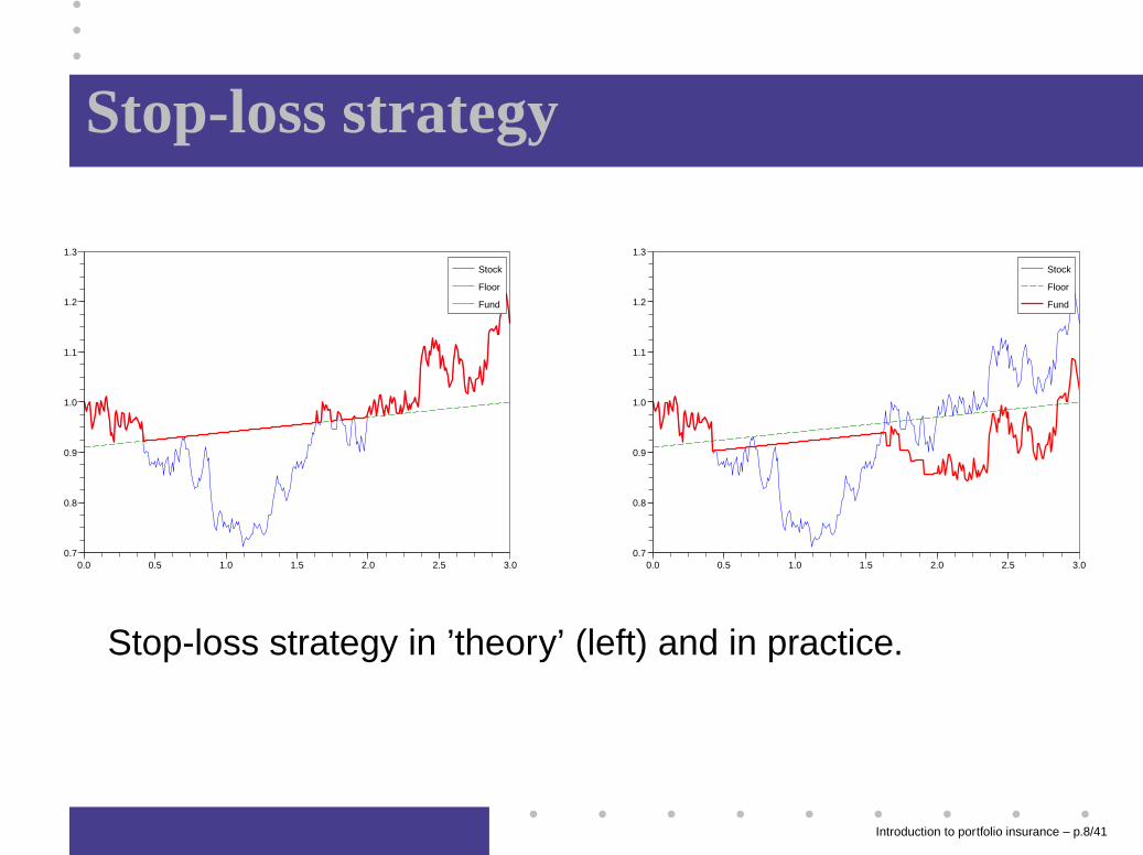
Stop-loss strategy in ’theory’ (left) and in practice.
Introduction to portfolio insurance – p.8/41
The loss is not stopped
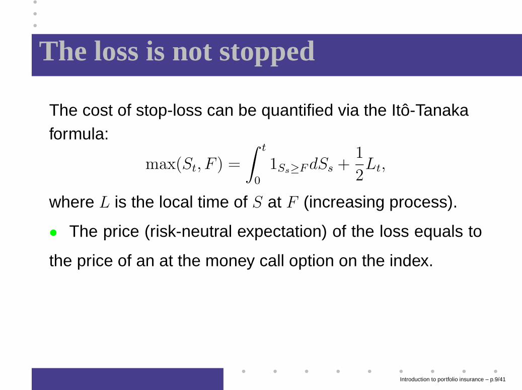
The cost of stop-loss can be quantified via the Itô-Tanakaformula:
max(St, F ) =
∫ t
0
1Ss≥F dSs +1
2Lt,
where L is the local time of S at F (increasing process).
• The price (risk-neutral expectation) of the loss equals to
the price of an at the money call option on the index.
Introduction to portfolio insurance – p.9/41

Option-based portfolio insurance
Introduction to portfolio insurance – p.10/41
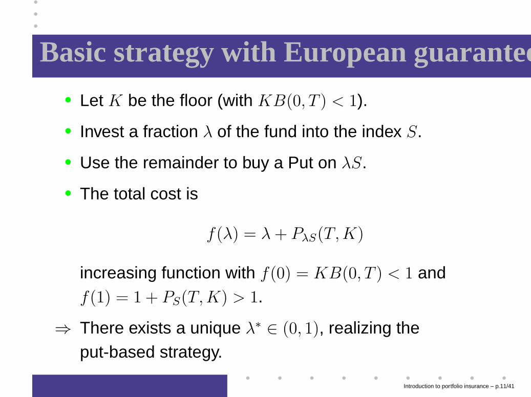
Basic strategy with European guarantee• Let K be the floor (with KB(0, T ) < 1).
• Invest a fraction λ of the fund into the index S.
• Use the remainder to buy a Put on λS.
• The total cost is
f(λ) = λ + PλS(T,K)
increasing function with f(0) = KB(0, T ) < 1 andf(1) = 1 + PS(T,K) > 1.
⇒ There exists a unique λ∗ ∈ (0, 1), realizing theput-based strategy.
Introduction to portfolio insurance – p.11/41
Optimality of the put-based strategy
Let u(x) = x1−γ
1−γand let ST be the optimal unconstrained
portfolio:
E[u(ST )] = maxE[u(XT )] subject to X0 = 1.
Then the put-based strategy is the optimal strategy subject
to the floor constraint (El Karoui, Jeanblanc, Lacoste ’05).
Introduction to portfolio insurance – p.12/41
Equivalent strategy using calls
By put-call parity, the put-based strategy is equivalent to:
• Buy zero-coupon with notional K to lock in the capitalat maturity
• Use the remainder to buy a call on λ∗ST with strike K
(or anything else!).
• Often, at-the-money calls are used; fund’s performanceis then proportional to the risky asset performance:
VT = 1 + k(ST − 1)+, k =1 − B(0, T )
C(T )< 1.
k is called gearing or indexation.
Introduction to portfolio insurance – p.13/41
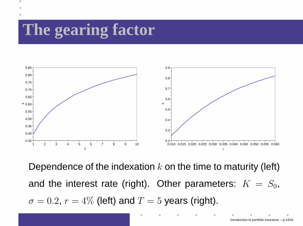
The gearing factor
1 2 3 4 5 6 7 8 9 100.35
0.40
0.45
0.50
0.55
0.60
0.65
0.70
0.75
0.80
0.85
T
k
0.010 0.015 0.020 0.025 0.030 0.035 0.040 0.045 0.050 0.055 0.0600.2
0.3
0.4
0.5
0.6
0.7
0.8
0.9
r
k
Dependence of the indexation k on the time to maturity (left)
and the interest rate (right). Other parameters: K = S0,
σ = 0.2, r = 4% (left) and T = 5 years (right).
Introduction to portfolio insurance – p.14/41
American capital guarantee• One cannot simply buy and hold an American put
because it is not self-financing.
• The correct strategy is dynamic trading in S andAmerican puts on S:
Vt = λtSt + P a(t, λtSt), λt = λ0 ∨ supu≤t
(
b(u)
Su
)
,
where b(t) is the exercise boundary and λ0 is chosenfrom the budget constraint.
• This self-financing strategy, satisfies Vt ≥ K, 0 ≤ t ≤ T
and is optimal for power utility in complete markets (EKJL).
Introduction to portfolio insurance – p.15/41
Replicating options
Danger of the OBPI approach: absence of liquid optionsfor long maturities (especially in the credit world)
• Counterparty risk if the option is boughtover-the-counter
• Marking-to-market difficult at intermediate dates
Common solution: replicate the option with a self-financing
portfolio containing ∆(St) stocks.
Introduction to portfolio insurance – p.16/41
OBPI with option replication
Advantages:
• No need to structure a long-dated option
• The portfolio is easy to mark to market and liquidate
Drawbacks:
• The replication is only approximate, especially inincomplete markets
• Transaction costs may be high
• Model-dependent
Introduction to portfolio insurance – p.17/41

Constant proportion portfolioinsurance
Introduction to portfolio insurance – p.18/41
The basic CPPI strategy
• Introduced by Black and Jones (87) and Perold (86).
• A fixed amount N is guaranteed at maturity T .
• At every t, a fraction is invested into risky asset St andthe remainder into zero-coupon bond with maturity T
and nominal N (denoted by Bt).
• If Vt > Bt, the risky asset exposure ismCt ≡ m(Vt − Bt), with m > 1.
• If Vt ≤ Bt, the entire portfolio is invested into thezero-coupon.
Introduction to portfolio insurance – p.19/41
Features and extensions
• Model-independent (for continuous processes).
• Maturity-independent, open-entry and open-exit.
• Greater upward potential than OBPI: while in OBPI theexposure is limited to the indexation k < 1, the CPPIexposure in bullish markets is only limited by themultiplier.
• Variable floor (ratchet) easily incorporated.
Introduction to portfolio insurance – p.20/41
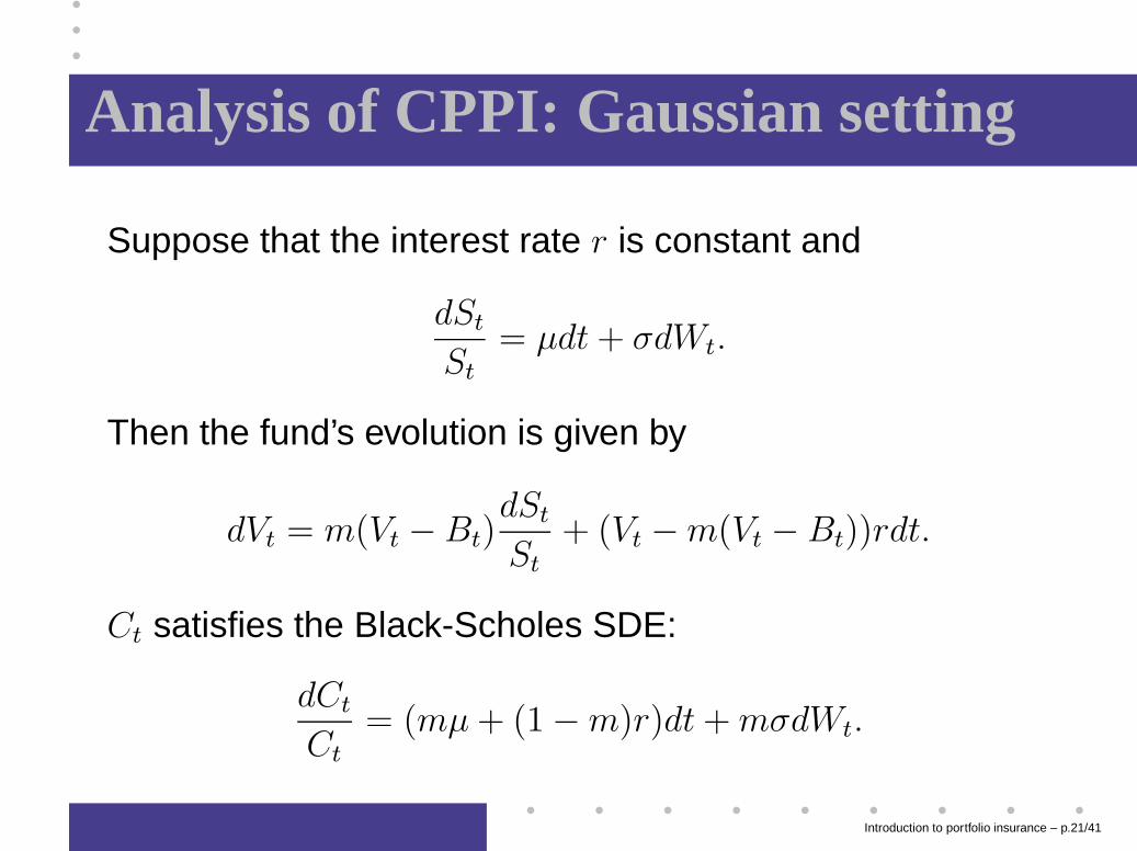
Analysis of CPPI: Gaussian setting
Suppose that the interest rate r is constant and
dSt
St= µdt + σdWt.
Then the fund’s evolution is given by
dVt = m(Vt − Bt)dSt
St
+ (Vt − m(Vt − Bt))rdt.
Ct satisfies the Black-Scholes SDE:
dCt
Ct
= (mµ + (1 − m)r)dt + mσdWt.
Introduction to portfolio insurance – p.21/41
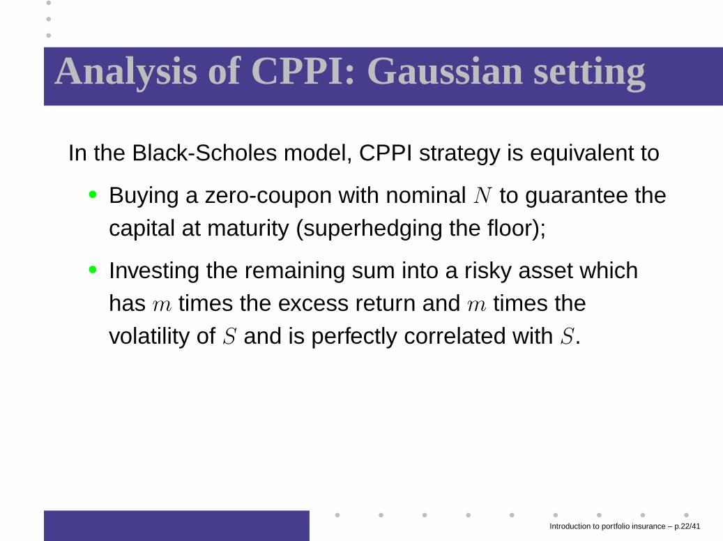
Analysis of CPPI: Gaussian setting
In the Black-Scholes model, CPPI strategy is equivalent to
• Buying a zero-coupon with nominal N to guarantee thecapital at maturity (superhedging the floor);
• Investing the remaining sum into a risky asset whichhas m times the excess return and m times thevolatility of S and is perfectly correlated with S.
Introduction to portfolio insurance – p.22/41
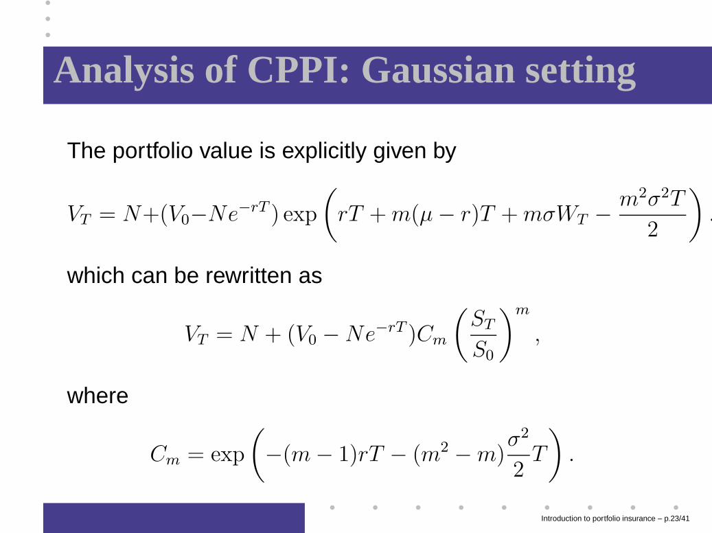
Analysis of CPPI: Gaussian setting
The portfolio value is explicitly given by
VT = N+(V0−Ne−rT ) exp
(
rT + m(µ − r)T + mσWT − m2σ2T
2
)
.
which can be rewritten as
VT = N + (V0 − Ne−rT )Cm
(
ST
S0
)m
,
where
Cm = exp
(
−(m − 1)rT − (m2 − m)σ2
2T
)
.
Introduction to portfolio insurance – p.23/41
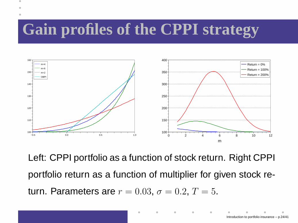
Gain profiles of the CPPI strategy
−0.5 0.0 0.5 1.0100
110
120
130
140
150
160
m=4
m=6
m=2
OBPI
0 2 4 6 8 10 12100
150
200
250
300
350
400
m
Return = 0%
Return = 100%
Return = 200%
Left: CPPI portfolio as a function of stock return. Right CPPI
portfolio return as a function of multiplier for given stock re-
turn. Parameters are r = 0.03, σ = 0.2, T = 5.
Introduction to portfolio insurance – p.24/41
Optimality of CPPI
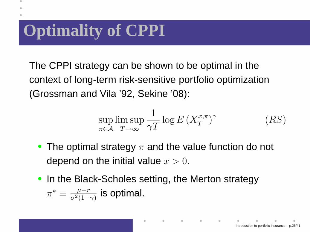
The CPPI strategy can be shown to be optimal in thecontext of long-term risk-sensitive portfolio optimization(Grossman and Vila ’92, Sekine ’08):
supπ∈A
lim supT→∞
1
γTlog E (Xx,π
T )γ (RS)
• The optimal strategy π and the value function do notdepend on the initial value x > 0.
• In the Black-Scholes setting, the Merton strategyπ∗ ≡ µ−r
σ2(1−γ)is optimal.
Introduction to portfolio insurance – p.25/41
Optimality of CPPI
For the problem (RS) under the constraint Xx,πt ≥ Kt for all
t, an optimal strategy is described by
• Superhedge the floor process with any portfolio K̄
satisfying K̄0 < x.
• Invest x − K̄0 into the unconstrained optimal portfolio.
In the Black-Scholes model ⇒ classical CPPI withmultiplier given by the Merton portfolio π∗.
• Extension by Grossman and Zhou ’93 and Cvitanic andKaratzas ’96: the CPPI strategy with stochastic floor isoptimal for (RS) in case of drawdown constraints.
Introduction to portfolio insurance – p.26/41
Optimality of CPPI: critique
• Merton’s multiplier may be too low: it results from theunconstrained problem which takes into account bothgains and losses, and under the floor constraintinvestors accept greater risks to maximize gains.
• In models with jumps, the positivity constraint oftenimplies 0 ≤ π ≤ 1, which is not sufficient for CPPI ⇒one may want to authorise some gap risk ⇒optimisation under VaR constraint.
• Market practice is to use basic CPPI with m fixed asfunction of the VaR constraint.
Introduction to portfolio insurance – p.27/41

Some explicit computations forCPPI with jumps
Introduction to portfolio insurance – p.28/41
Introducing jumps
Suppose that S and B may be written as
dSt
St−= dZt and
dBt
Bt= dRt,
where Z is a semimartingale with ∆Z > −1 and R is acontinuous semimartingale.This implies
Bt = B0 exp
(
Rt −1
2[R]t
)
> 0.
Example: Rt = rt and Z is a Lévy process.
Introduction to portfolio insurance – p.29/41
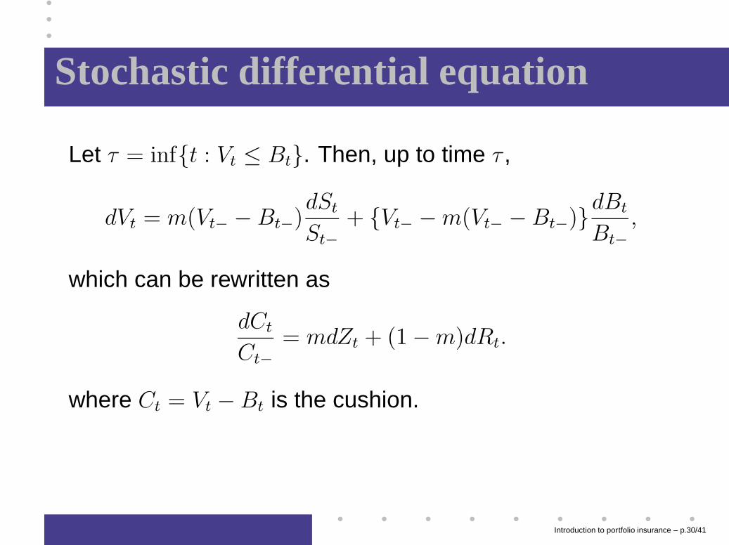
Stochastic differential equation
Let τ = inf{t : Vt ≤ Bt}. Then, up to time τ ,
dVt = m(Vt− − Bt−)dSt
St−
+ {Vt− − m(Vt− − Bt−)}dBt
Bt−
,
which can be rewritten as
dCt
Ct−
= mdZt + (1 − m)dRt.
where Ct = Vt − Bt is the cushion.
Introduction to portfolio insurance – p.30/41
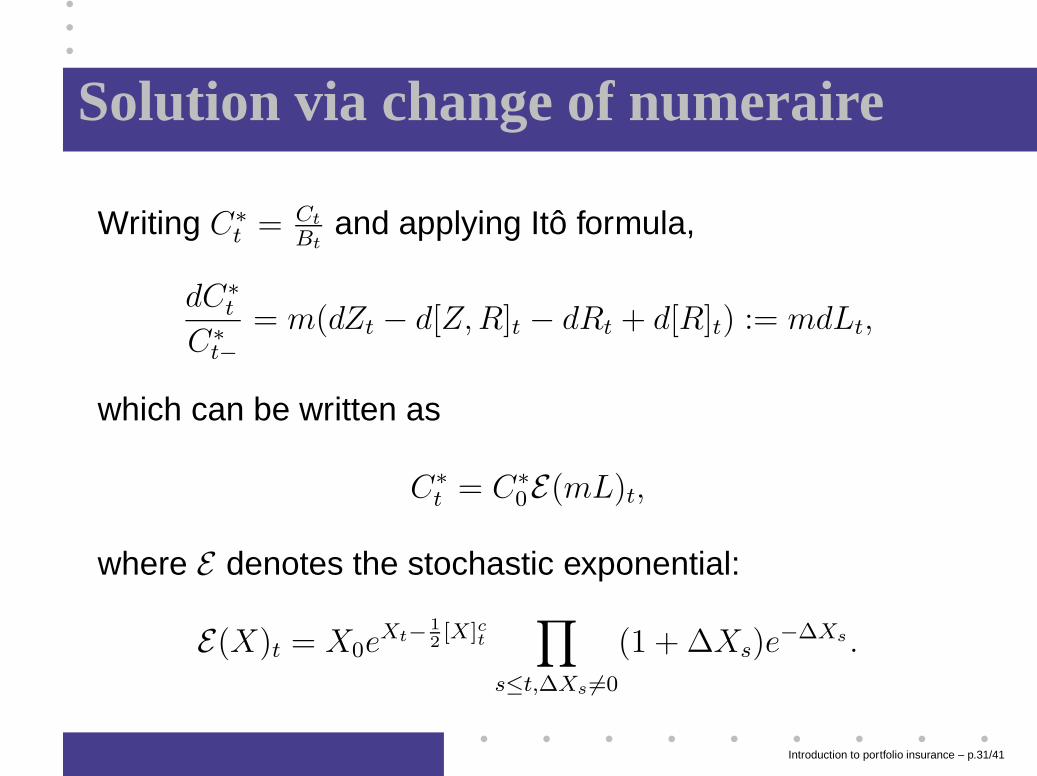
Solution via change of numeraire
Writing C∗t = Ct
Btand applying Itô formula,
dC∗t
C∗t−
= m(dZt − d[Z,R]t − dRt + d[R]t) := mdLt,
which can be written as
C∗t = C∗
0E(mL)t,
where E denotes the stochastic exponential:
E(X)t = X0eXt−
1
2[X]ct
∏
s≤t,∆Xs 6=0
(1 + ∆Xs)e−∆Xs .
Introduction to portfolio insurance – p.31/41
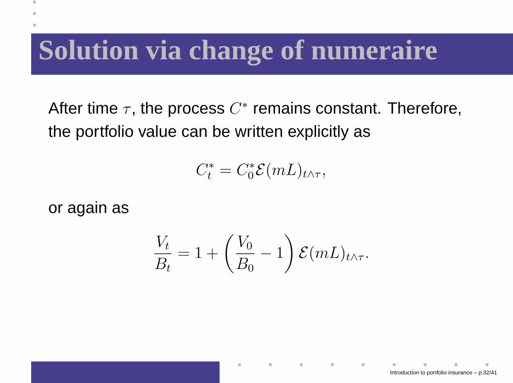
Solution via change of numeraire
After time τ , the process C∗ remains constant. Therefore,the portfolio value can be written explicitly as
C∗t = C∗
0E(mL)t∧τ ,
or again as
Vt
Bt= 1 +
(
V0
B0− 1
)
E(mL)t∧τ .
Introduction to portfolio insurance – p.32/41
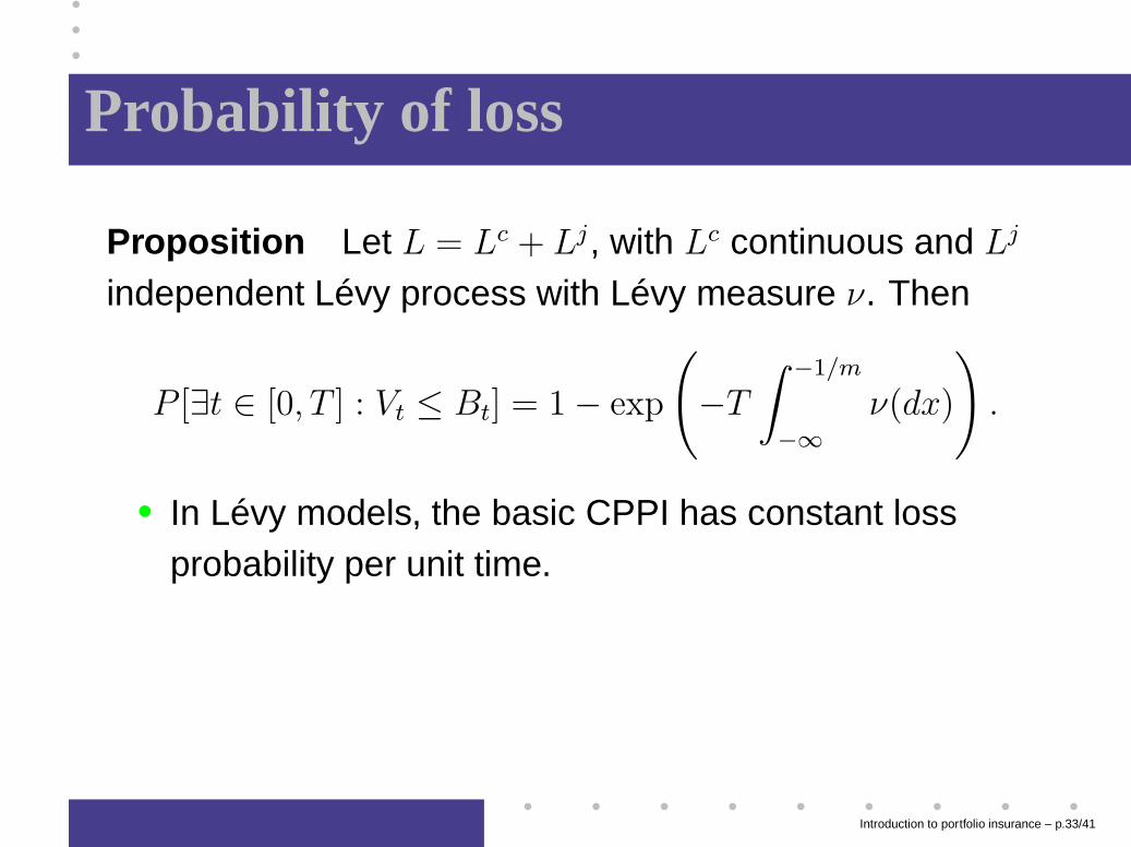
Probability of loss
Proposition Let L = Lc + Lj, with Lc continuous and Lj
independent Lévy process with Lévy measure ν. Then
P [∃t ∈ [0, T ] : Vt ≤ Bt] = 1 − exp
(
−T
∫ −1/m
−∞
ν(dx)
)
.
• In Lévy models, the basic CPPI has constant lossprobability per unit time.
Introduction to portfolio insurance – p.33/41
Probability of loss
Proof: Vt ≤ Bt ⇐⇒ C∗t ≤ 0 ⇐⇒
C∗t = C∗
0E(mL)t ≤ 0.
But since
∆E(X)t = E(X)t−(1 + ∆Xt),
this is equivalent to ∆Ljt ≤ −1/m.
For a Lévy process Lj, the number of such jumps in the
interval [0, T ] is a Poisson random variable with intensity
T∫ −1/m
−∞ν(dx).
Introduction to portfolio insurance – p.34/41
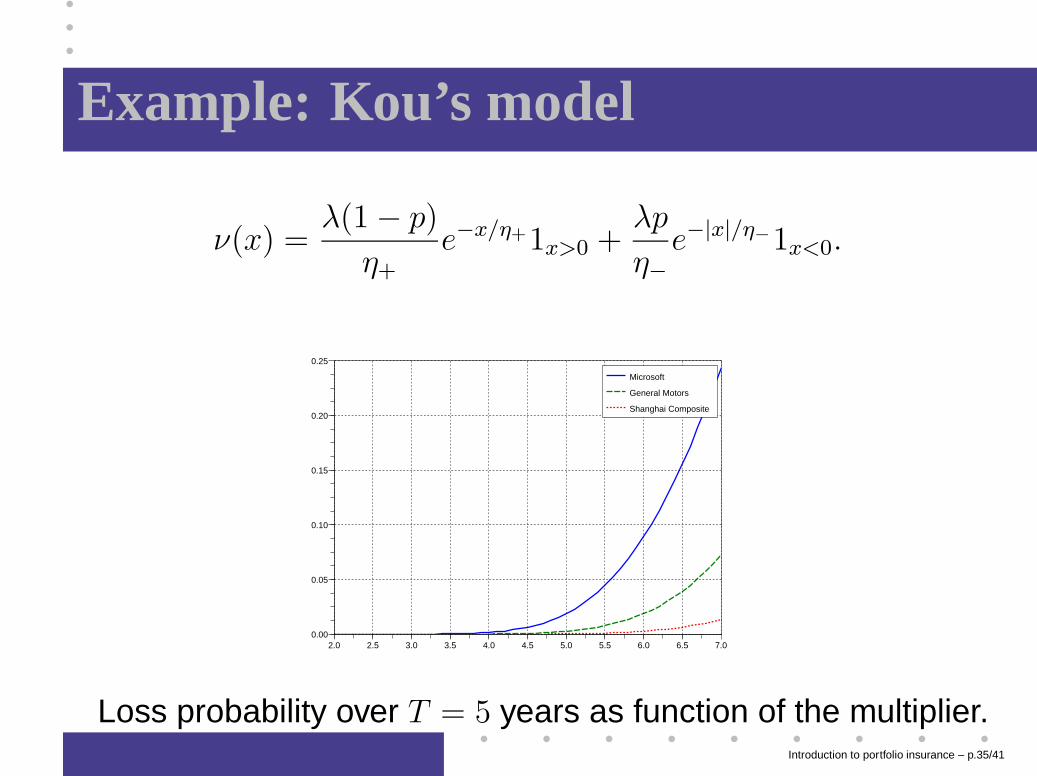
Example: Kou’s model
ν(x) =λ(1 − p)
η+e−x/η+1x>0 +
λp
η−e−|x|/η
−1x<0.
2.0 2.5 3.0 3.5 4.0 4.5 5.0 5.5 6.0 6.5 7.00.00
0.05
0.10
0.15
0.20
0.25
Microsoft
General Motors
Shanghai Composite
Loss probability over T = 5 years as function of the multiplier.Introduction to portfolio insurance – p.35/41

Stochastic volatility and variablemultiplier strategies
Introduction to portfolio insurance – p.36/41
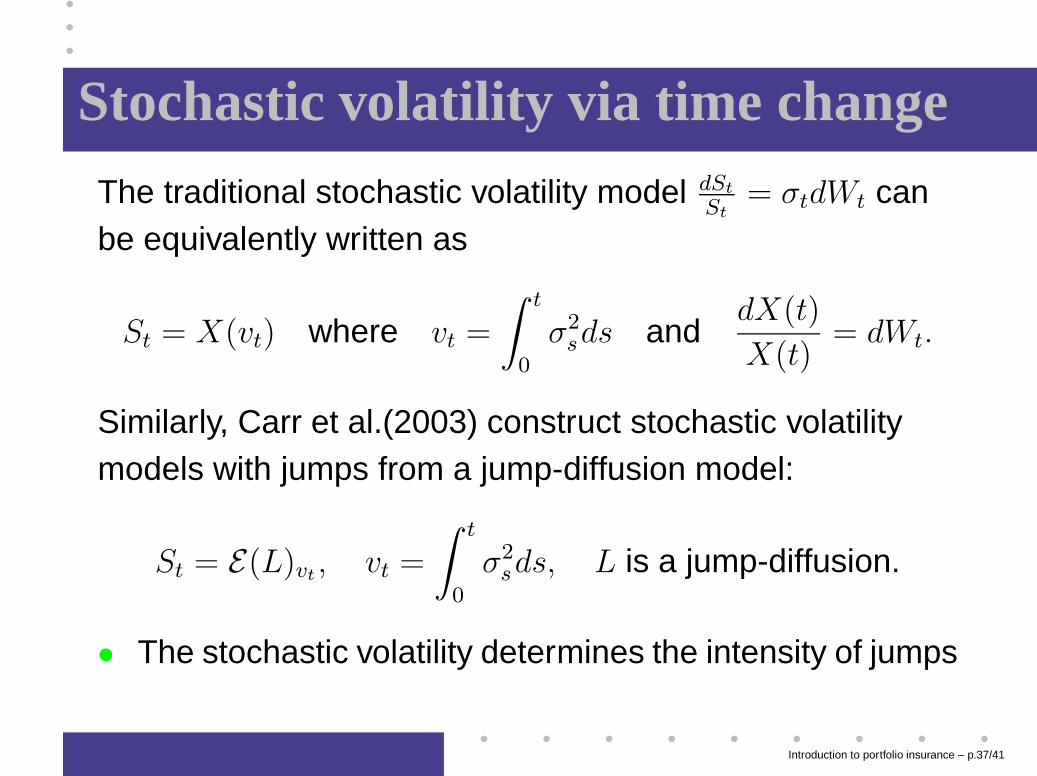
Stochastic volatility via time change
The traditional stochastic volatility model dSt
St= σtdWt can
be equivalently written as
St = X(vt) where vt =
∫ t
0
σ2sds and
dX(t)
X(t)= dWt.
Similarly, Carr et al.(2003) construct stochastic volatilitymodels with jumps from a jump-diffusion model:
St = E(L)vt , vt =
∫ t
0
σ2sds, L is a jump-diffusion.
• The stochastic volatility determines the intensity of jumps
Introduction to portfolio insurance – p.37/41
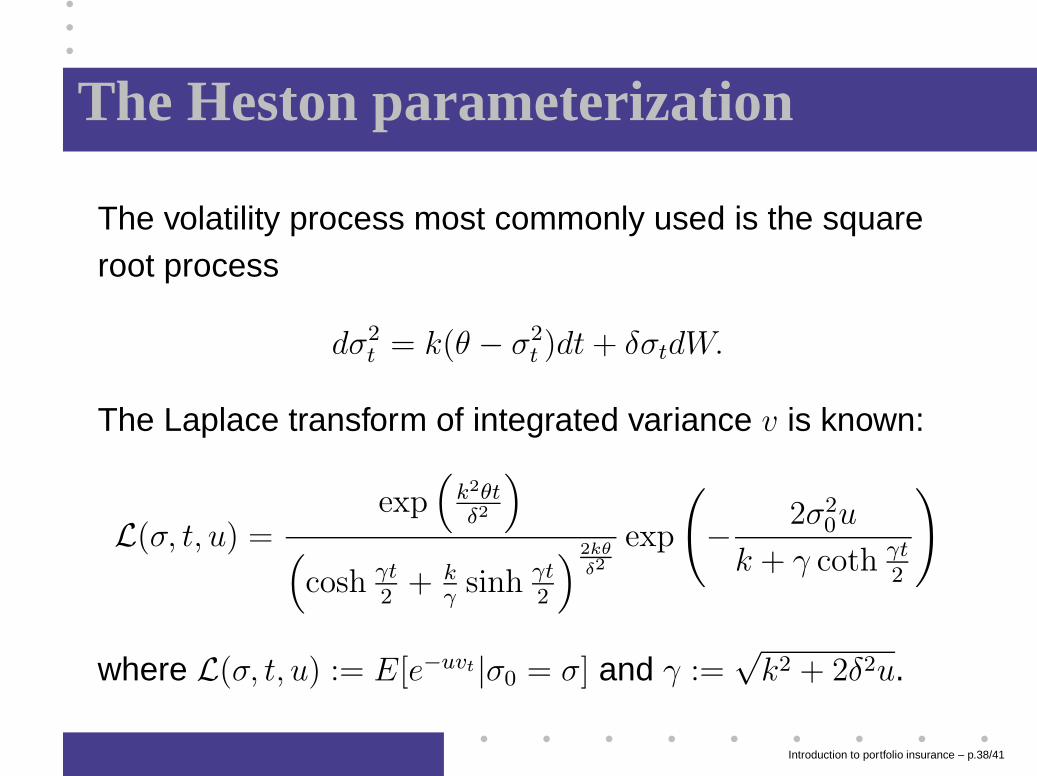
The Heston parameterization
The volatility process most commonly used is the squareroot process
dσ2t = k(θ − σ2
t )dt + δσtdW.
The Laplace transform of integrated variance v is known:
L(σ, t, u) =exp
(
k2θtδ2
)
(
cosh γt2
+ kγ
sinh γt2
)2kθ
δ2
exp
(
− 2σ20u
k + γ coth γt2
)
where L(σ, t, u) := E[e−uvt|σ0 = σ] and γ :=√
k2 + 2δ2u.
Introduction to portfolio insurance – p.38/41
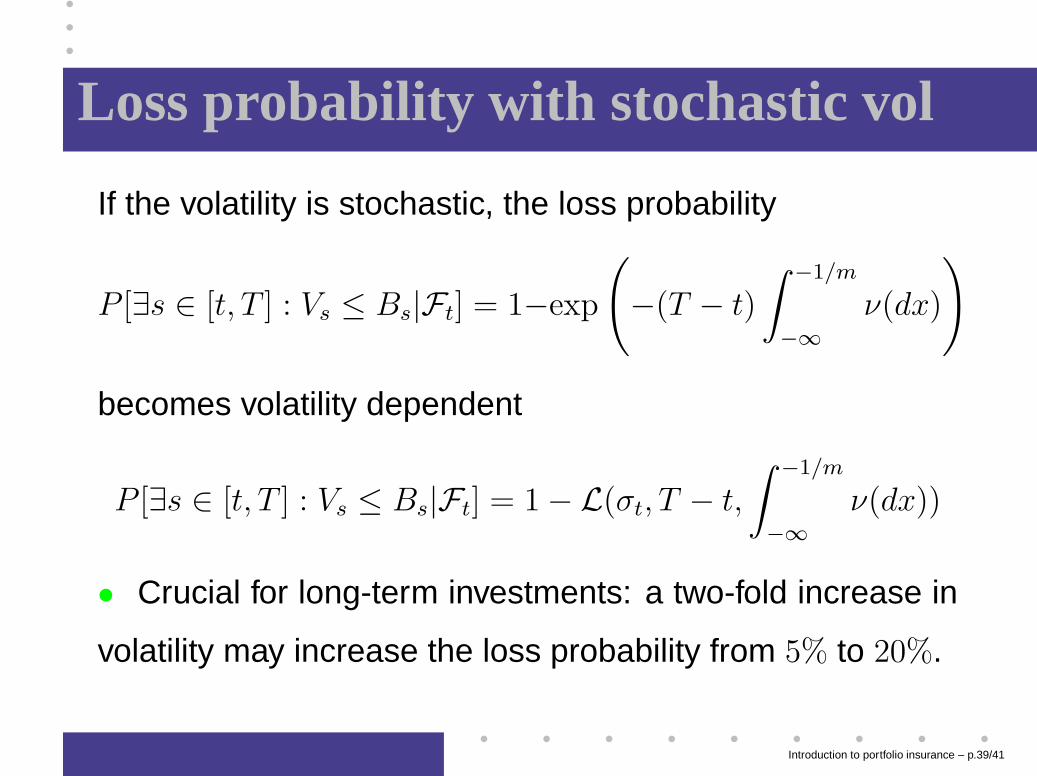
Loss probability with stochastic vol
If the volatility is stochastic, the loss probability
P [∃s ∈ [t, T ] : Vs ≤ Bs|Ft] = 1−exp
(
−(T − t)
∫ −1/m
−∞
ν(dx)
)
becomes volatility dependent
P [∃s ∈ [t, T ] : Vs ≤ Bs|Ft] = 1 − L(σt, T − t,
∫ −1/m
−∞
ν(dx))
• Crucial for long-term investments: a two-fold increase in
volatility may increase the loss probability from 5% to 20%.
Introduction to portfolio insurance – p.39/41
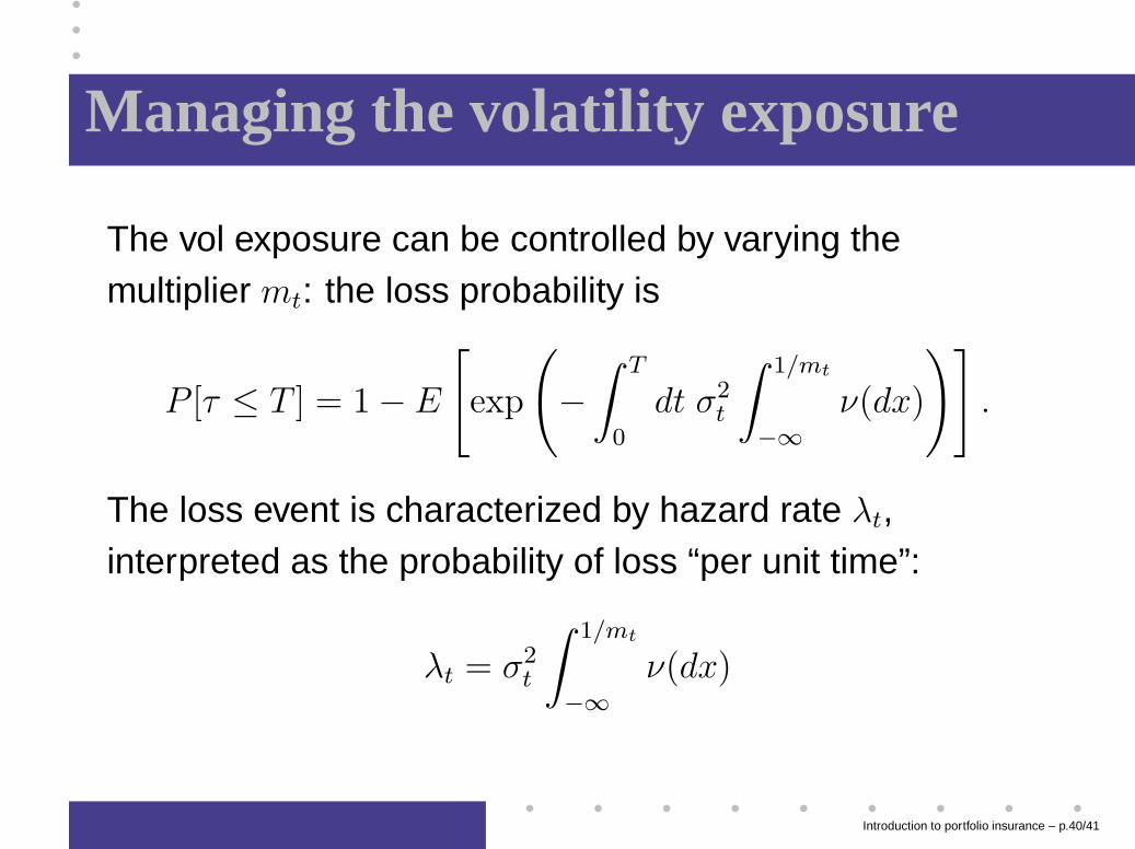
Managing the volatility exposure
The vol exposure can be controlled by varying themultiplier mt: the loss probability is
P [τ ≤ T ] = 1 − E
[
exp
(
−∫ T
0
dt σ2t
∫ 1/mt
−∞
ν(dx)
)]
.
The loss event is characterized by hazard rate λt,interpreted as the probability of loss “per unit time”:
λt = σ2t
∫ 1/mt
−∞
ν(dx)
Introduction to portfolio insurance – p.40/41
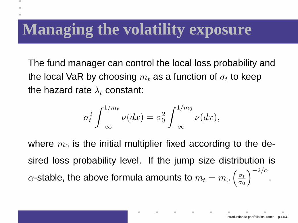
Managing the volatility exposure
The fund manager can control the local loss probability andthe local VaR by choosing mt as a function of σt to keepthe hazard rate λt constant:
σ2t
∫ 1/mt
−∞
ν(dx) = σ20
∫ 1/m0
−∞
ν(dx),
where m0 is the initial multiplier fixed according to the de-
sired loss probability level. If the jump size distribution is
α-stable, the above formula amounts to mt = m0
(
σt
σ0
)−2/α
.
Introduction to portfolio insurance – p.41/41


![NATIONAL HOSPITAL INSURANCE FUND ACT Hospital Insurance Fund Act.pdf · LAWS OF KENYA NATIONAL HOSPITAL INSURANCE FUND ACT CHAPTER 255 Revised Edition 2012 [1998] Published by the](https://img.pdfslide.us/doc/110x75/5e12f81a5e1d572ccb627d42/national-hospital-insurance-fund-act-hospital-insurance-fund-actpdf-laws-of-kenya.jpg)