Introduction to Polar Coordinates in Mechanics (for AQA Mechanics 5) Until now, we have dealt with displacement, velocity and acceleration in Cartesian coordinates - that is, in relation to fixed perpendicular directions defined by the unit vectors and . Consider this exam question to be reminded how well this system works for circular motion: AQA Mechanics 2B, Jun ’12

Note that the position vector is given in , form, with each component in terms of the time . To prove that the particle is performing circular motion about the origin, it is sufficient to show that the distance from the origin is constant. Since is the displacement vector, the distance is given by :

By considering how the and components vary as varies between and , we can get an

impression not just of position, but also of velocity. Eg, while

the particle is in the

fourth quadrant – in the direction the position is positive but decreasing slowly, and in the direction the position is negative and decreasing rapidly. In other words, the particle is travelling clockwise around a circle of radius about the origin, starting from the point .

Recall that the velocity can be found from displacement using the result

, and when

and are vectors, this means differentiating the and components separately, with respect to time (these components are perpendicular, so do not directly affect one another).

By considering the components of velocity at various points, just as we did for displacement,

we can get an idea of the velocity of the particle. For instance, when

, the particle is

moving left (quickly at first, but with decreasing speed) and up (slowly at first, but with increasing speed). Note also that, using the same method as in part a), we could use Pythagoras to show that the magnitude of velocity (the speed) is constant. Therefore while direction is constantly changing, the particle is travelling at a constant speed. Since the acceleration of the particle is affecting both components of velocity, it is harder to see how this is changing directly from this expression, but it will become clearer once we find the acceleration vector. Note, however, that as the component of velocity increases, the component decreases and vice versa. We should find that the acceleration of the particle is of constant magnitude even though its direction is constantly changing.

Recall that the acceleration vector can be found from velocity using the result

.

Note firstly that it would be easy to show, as in part a), that acceleration is constant in magnitude (if not direction). Also note the similarity of this expression to that of displacement. The only difference is the signs (negative and positive in this case) and the magnitude. So the acceleration is clearly directly related to the displacement of the particle. This is a key feature of circular motion.

This is a straightforward result to prove, but it is crucial to the idea of circular motion.

Since the acceleration vector is a scalar multiple of the displacement vector, the two vectors are parallel. This means acceleration always acts along the same line as the displacement of the particle from the origin (that is, along the radius of the circular motion).

Note the negative sign – this tells us that the acceleration acts in the opposite direction to displacement. Displacement measures the position of the particle relative to the origin, and so it always points from the origin to the particle. Therefore acceleration points from the particle to the origin. This fits in with the whole concept of centripetal force and centripetal acceleration. Since the velocity is constantly changing direction, the acceleration vector must be constantly changing direction, and since acceleration is always pointing radially (towards the centre), it cannot affect the magnitude of velocity which always points tangentially (at right angles to the radial direction).

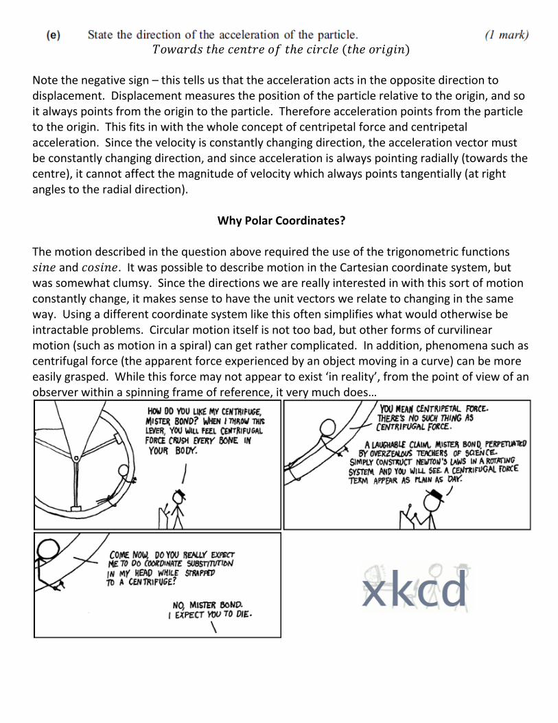
Why Polar Coordinates? The motion described in the question above required the use of the trigonometric functions and . It was possible to describe motion in the Cartesian coordinate system, but was somewhat clumsy. Since the directions we are really interested in with this sort of motion constantly change, it makes sense to have the unit vectors we relate to changing in the same way. Using a different coordinate system like this often simplifies what would otherwise be intractable problems. Circular motion itself is not too bad, but other forms of curvilinear motion (such as motion in a spiral) can get rather complicated. In addition, phenomena such as centrifugal force (the apparent force experienced by an object moving in a curve) can be more easily grasped. While this force may not appear to exist ‘in reality’, from the point of view of an observer within a spinning frame of reference, it very much does…

Constructing the Polar Coordinate System A note on notation To stop an already complicated system of formulae looking completely ludicrous, we will use

the accepted notation

and

. These are the derivative and second derivative of

(which is a function of ) with respect to . For instance, if then and . Implications of implicit differentiation Recall that if we need to differentiate an expression in terms of one variable with respect to

another, the chain rule allows us to write:

.

Combining this idea with the notation above, we can say things like:

.

Note that, like any letters used here which aren’t vectors, is a function of time. When a letter represents a vector, it will be written in bold. The Cartesian system We begin by considering what we already know – the Cartesian system: The general form of displacement would be given as: where and are functions of time, and and are fixed perpendicular unit vectors in the plane. The velocity vector can found from displacement: Since velocity is the rate of change of displacement, it can be described precisely, in vector form, by considering the rate of change separately in each of the two fixed perpendicular directions. Similarly, the acceleration vector can be found: Note the use of and for the velocity and acceleration vectors. The results above are the definitions of these vectors, and their derivatives cannot be found directly, but depend on these definitions. This will become important – and less intuitive – when we define equivalent expressions for displacement ( ), velocity ( ) and acceleration ( ) in polar coordinates.

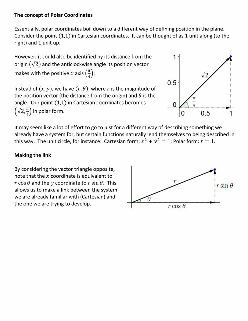
The concept of Polar Coordinates Essentially, polar coordinates boil down to a different way of defining position in the plane. Consider the point in Cartesian coordinates. It can be thought of as unit along (to the right) and unit up. However, it could also be identified by its distance from the

origin and the anticlockwise angle its position vector

makes with the positive axis

:

Instead of , we have , where is the magnitude of the position vector (the distance from the origin) and is the angle. Our point in Cartesian coordinates becomes

in polar form.

It may seem like a lot of effort to go to just for a different way of describing something we already have a system for, but certain functions naturally lend themselves to being described in this way. The unit circle, for instance: Cartesian form: ; Polar form: . Making the link By considering the vector triangle opposite, note that the coordinate is equivalent to and the coordinate to . This allows us to make a link between the system we are already familiar with (Cartesian) and the one we are trying to develop.

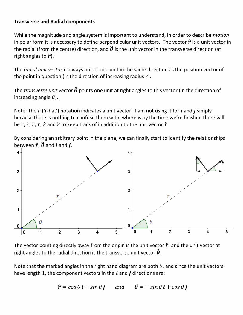
Transverse and Radial components While the magnitude and angle system is important to understand, in order to describe motion in polar form it is necessary to define perpendicular unit vectors. The vector is a unit vector in

the radial (from the centre) direction, and is the unit vector in the transverse direction (at right angles to ). The radial unit vector always points one unit in the same direction as the position vector of the point in question (in the direction of increasing radius ).

The transverse unit vector points one unit at right angles to this vector (in the direction of increasing angle ). Note: The (‘r-hat’) notation indicates a unit vector. I am not using it for and simply because there is nothing to confuse them with, whereas by the time we’re finished there will be , , , , and to keep track of in addition to the unit vector . By considering an arbitrary point in the plane, we can finally start to identify the relationships

between , and and .

The vector pointing directly away from the origin is the unit vector , and the unit vector at

right angles to the radial direction is the transverse unit vector . Note that the marked angles in the right hand diagram are both , and since the unit vectors have length , the component vectors in the and directions are:

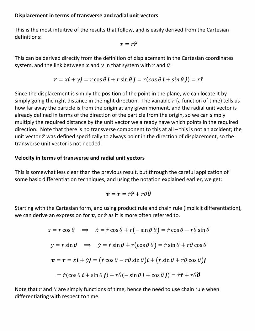
Displacement in terms of transverse and radial unit vectors This is the most intuitive of the results that follow, and is easily derived from the Cartesian definitions:

This can be derived directly from the definition of displacement in the Cartesian coordinates system, and the link between and in that system with and :

Since the displacement is simply the position of the point in the plane, we can locate it by simply going the right distance in the right direction. The variable (a function of time) tells us how far away the particle is from the origin at any given moment, and the radial unit vector is already defined in terms of the direction of the particle from the origin, so we can simply multiply the required distance by the unit vector we already have which points in the required direction. Note that there is no transverse component to this at all – this is not an accident; the unit vector was defined specifically to always point in the direction of displacement, so the transverse unit vector is not needed. Velocity in terms of transverse and radial unit vectors This is somewhat less clear than the previous result, but through the careful application of some basic differentiation techniques, and using the notation explained earlier, we get:

Starting with the Cartesian form, and using product rule and chain rule (implicit differentiation), we can derive an expression for , or as it is more often referred to.

Note that and are simply functions of time, hence the need to use chain rule when differentiating with respect to time.

We designed our coordinate system with displacement in mind, which is why the displacement vector is so straightforward (there is never any transverse component). However, this means that the form we arrive at for velocity takes a little explaining. Fortunately, when broken down, it is not a huge step from the idea of velocity in circular motion. Note first of all that the radial component of velocity is simply – the rate of change of the radial distance. If the particle is moving directly away from the centre (and not changing its angle at all), this is the only component of velocity it would have.

Secondly, in order to understand the transverse component we should consider what represents – it is the rate of change of the angle, , with respect to time. In other words, the angular velocity of the particle, which is often written as . When measuring the overall velocity of a particle, we need to take into account its velocity in both directions (radial and tangential/transverse). The radial velocity is the rate at which the radius is changing, , and the transverse speed must be the rate at which it is moving at right angles to the radius. Just as tangential speed in circular motion is given by , so our tangential speed is

also , or, using our notation, . When the two components of velocity are combined, and written along with the radial and transverse unit vectors, we get:

Angular Velocity side note: Since the angular velocity measures radians turned through per second, it takes no account of the size of the circle. So the angular velocity of the Earth around the sun is microscopic because it takes a whole year just to complete a single turn ( radians in 31.5 million seconds, or ), while the angular velocity of a PowerBall gyroscope might easily be 10,000 rpm ( radians in seconds, or ). Since a turn of one radian represents an arc length of exactly one radius-length, multiplying the angular velocity by the radius gives the actual speed (in ).

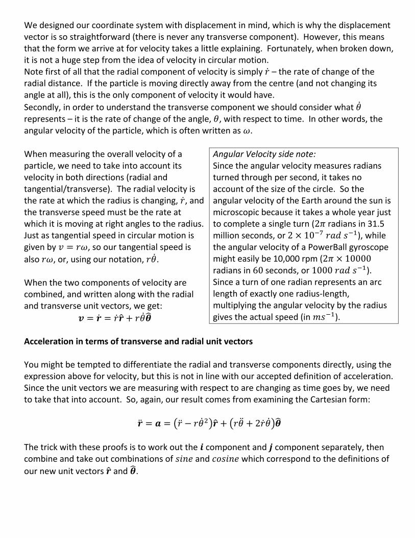
Acceleration in terms of transverse and radial unit vectors You might be tempted to differentiate the radial and transverse components directly, using the expression above for velocity, but this is not in line with our accepted definition of acceleration. Since the unit vectors we are measuring with respect to are changing as time goes by, we need to take that into account. So, again, our result comes from examining the Cartesian form:

The trick with these proofs is to work out the component and component separately, then combine and take out combinations of and which correspond to the definitions of

our new unit vectors and .

The acceleration expression is the most complicated-looking of the three, but looking at the individual components in turn will enable us to identify the key components and how they fit in. Firstly, the radial component is the combined effect of the motion along the radial line and

centripetal acceleration. Note that which should be familiar from circular motion (also note that the term is negative since the centripetal force must act towards the origin).

Secondly, the transverse component is a combination of and . Taking the term first,

we should recognize that is the rate of change of angular velocity (since ), so it makes sense that it should form part of the transverse acceleration – if the velocity in the transverse direction is changing, the acceleration in that direction will depend on the rate of change of the transverse velocity. This effect is magnified if the particle is further from the origin – that is, when is large. So by multiplying by we get a term which provides part of the total

transverse acceleration. Next, to understand the term, we need to recognize that it comes about as a consequence of a change in transverse velocity. The previous term is simply the acceleration required at a given distance from the origin to change angular speed, but this term comes into effect when the radius (the distance from the origin) is also changing. It is directly

related to the angular velocity, hence the term, but since it depends on the rate at which the radius changes, it must also contain .

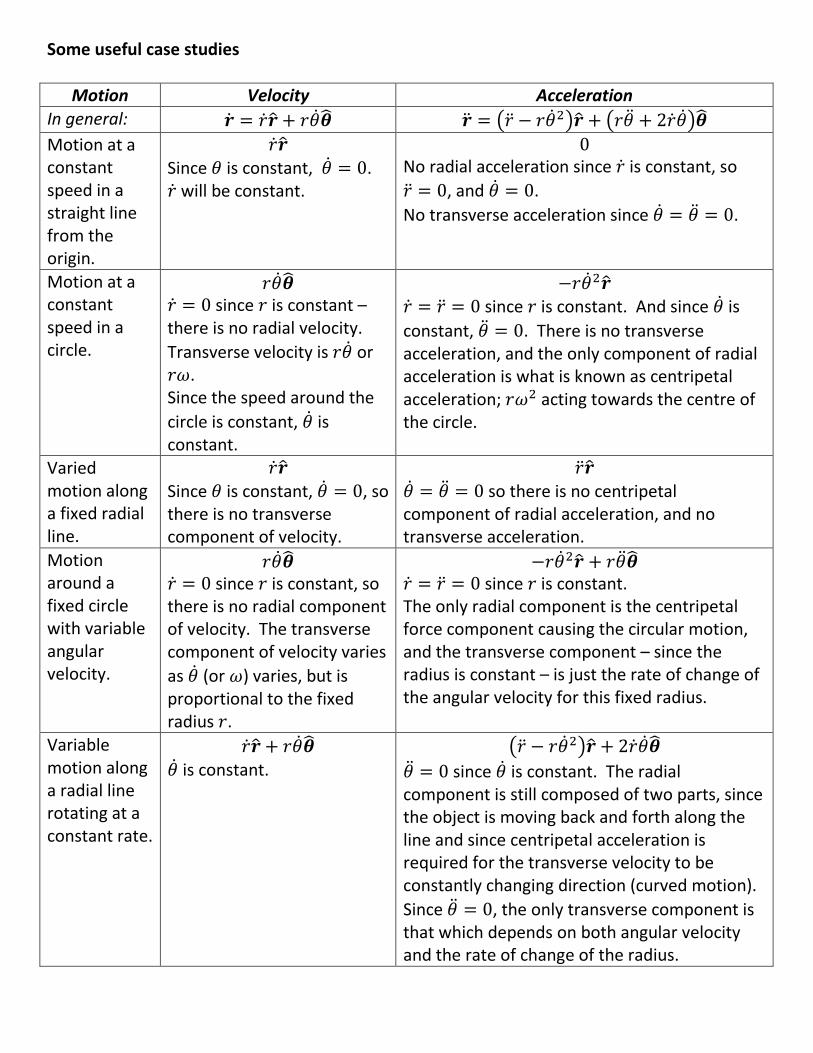
Some useful case studies

Motion Velocity Acceleration

In general:

Motion at a constant speed in a straight line from the origin.

Since is constant, . will be constant.

No radial acceleration since is constant, so

, and .

No transverse acceleration since .

Motion at a constant speed in a circle.

since is constant – there is no radial velocity.

Transverse velocity is or . Since the speed around the

circle is constant, is constant.

since is constant. And since is

constant, . There is no transverse acceleration, and the only component of radial acceleration is what is known as centripetal acceleration; acting towards the centre of the circle.

Varied motion along a fixed radial line.

Since is constant, , so there is no transverse component of velocity.

so there is no centripetal component of radial acceleration, and no transverse acceleration.

Motion around a fixed circle with variable angular velocity.

since is constant, so there is no radial component of velocity. The transverse component of velocity varies

as (or ) varies, but is proportional to the fixed radius .

since is constant. The only radial component is the centripetal force component causing the circular motion, and the transverse component – since the radius is constant – is just the rate of change of the angular velocity for this fixed radius.

Variable motion along a radial line rotating at a constant rate.

is constant.

since is constant. The radial component is still composed of two parts, since the object is moving back and forth along the line and since centripetal acceleration is required for the transverse velocity to be constantly changing direction (curved motion).

Since , the only transverse component is that which depends on both angular velocity and the rate of change of the radius.

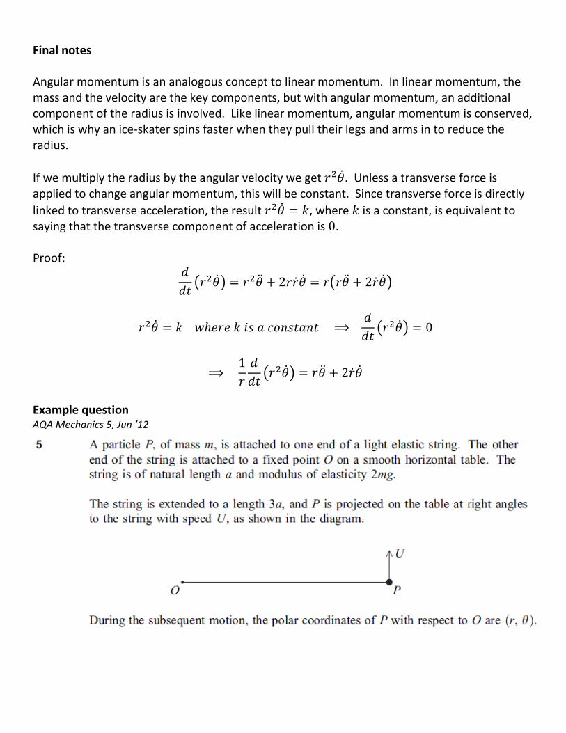
Final notes Angular momentum is an analogous concept to linear momentum. In linear momentum, the mass and the velocity are the key components, but with angular momentum, an additional component of the radius is involved. Like linear momentum, angular momentum is conserved, which is why an ice-skater spins faster when they pull their legs and arms in to reduce the radius.

If we multiply the radius by the angular velocity we get . Unless a transverse force is applied to change angular momentum, this will be constant. Since transverse force is directly

linked to transverse acceleration, the result , where is a constant, is equivalent to saying that the transverse component of acceleration is . Proof:

Example question AQA Mechanics 5, Jun ’12

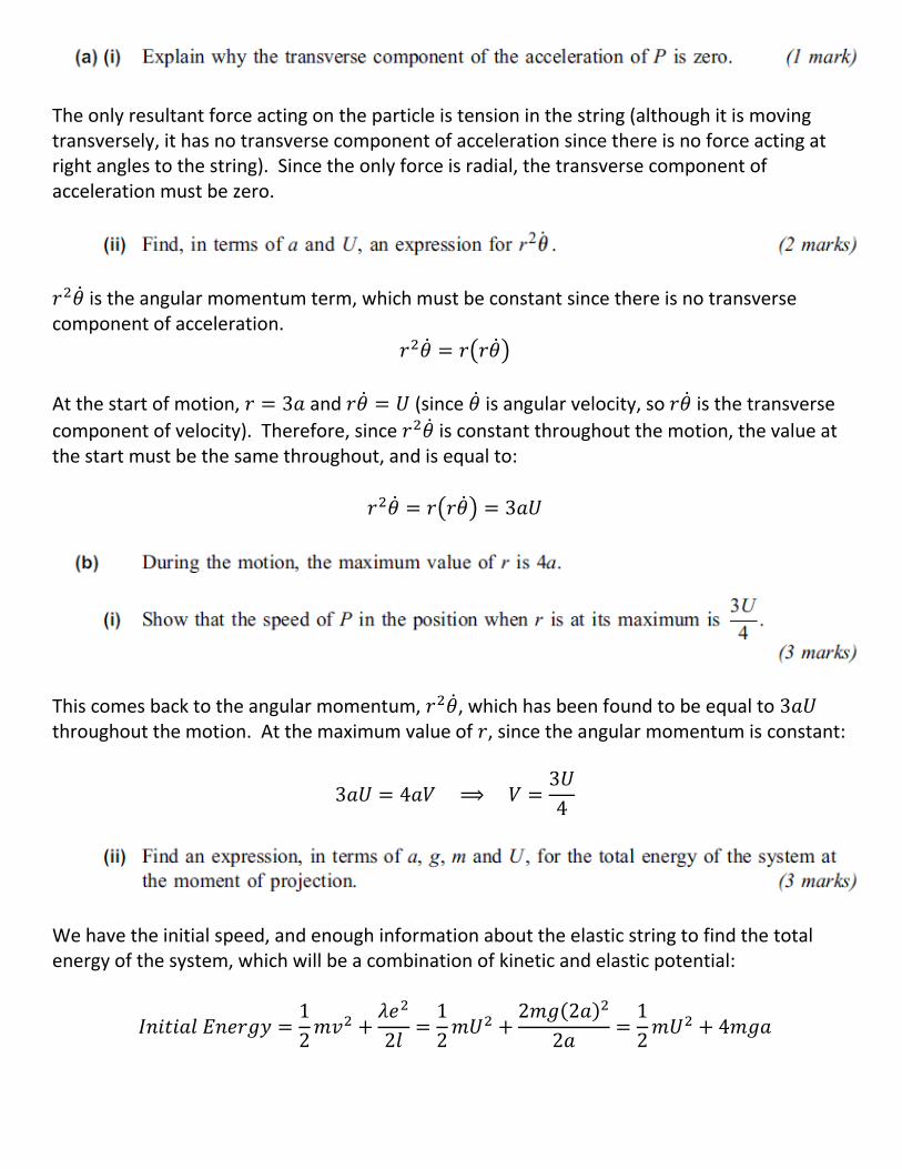
The only resultant force acting on the particle is tension in the string (although it is moving transversely, it has no transverse component of acceleration since there is no force acting at right angles to the string). Since the only force is radial, the transverse component of acceleration must be zero.

is the angular momentum term, which must be constant since there is no transverse component of acceleration.

At the start of motion, and (since is angular velocity, so is the transverse

component of velocity). Therefore, since is constant throughout the motion, the value at the start must be the same throughout, and is equal to:

This comes back to the angular momentum, , which has been found to be equal to throughout the motion. At the maximum value of , since the angular momentum is constant:

We have the initial speed, and enough information about the elastic string to find the total energy of the system, which will be a combination of kinetic and elastic potential:

At the point when is maximal:

Since energy is conserved:

Using Hooke’s law, at maximum stretch the tension will be

Since this is the resultant force acting on the particle, we can use to find the radial component of acceleration (and, as we have already established, there is no transverse

component).

. Note that this is pulling towards the centre, making the direction of

acceleration negative in relation to the radial unit vector. Additional note: Since, as we have already established, the transverse component of acceleration is zero, the direction must be purely radial. Radial acceleration is given by:

But since, at maximum , , , so this is simply . Since, using force and acceleration, we have already found this value, we could use our result to work backwards and find the angular velocity at this point: