Embed Size (px)
Citation preview
Introduction ToPhysical Oceanography
Robert H. StewartDepartment of Oceanography
Texas A & M University
Copyright 2003August 2003 Edition

ii

Contents
Preface vii
1 A Voyage of Discovery 11.1 Physics of the ocean . . . . . . . . . . . . . . . . . . . . . . . . . 11.2 Goals . . . . . . . . . . . . . . . . . . . . . . . . . . . . . . . . . 21.3 Organization . . . . . . . . . . . . . . . . . . . . . . . . . . . . . 31.4 The Big Picture . . . . . . . . . . . . . . . . . . . . . . . . . . . . 31.5 Further Reading . . . . . . . . . . . . . . . . . . . . . . . . . . . 4
2 The Historical Setting 72.1 Definitions . . . . . . . . . . . . . . . . . . . . . . . . . . . . . . . 82.2 Eras of Oceanographic Exploration . . . . . . . . . . . . . . . . . 82.3 Milestones in the Understanding of the Ocean . . . . . . . . . . . 112.4 Evolution of some Theoretical Ideas . . . . . . . . . . . . . . . . 152.5 The Role of Observations in Oceanography . . . . . . . . . . . . 162.6 Important Concepts . . . . . . . . . . . . . . . . . . . . . . . . . 19
3 The Physical Setting 213.1 Oceans and Seas . . . . . . . . . . . . . . . . . . . . . . . . . . . 223.2 Dimensions of the Oceans . . . . . . . . . . . . . . . . . . . . . . 233.3 Sea-Floor Features . . . . . . . . . . . . . . . . . . . . . . . . . . 253.4 Measuring the Depth of the Ocean . . . . . . . . . . . . . . . . . 293.5 Sea Floor Charts and Data Sets . . . . . . . . . . . . . . . . . . . 333.6 Sound in the Ocean . . . . . . . . . . . . . . . . . . . . . . . . . 353.7 Important Concepts . . . . . . . . . . . . . . . . . . . . . . . . . 37
4 Atmospheric Influences 394.1 The Earth in Space . . . . . . . . . . . . . . . . . . . . . . . . . . 394.2 Atmospheric Wind Systems . . . . . . . . . . . . . . . . . . . . . 414.3 The Planetary Boundary Layer . . . . . . . . . . . . . . . . . . . 434.4 Measurement of Wind . . . . . . . . . . . . . . . . . . . . . . . . 434.5 Calculations of Wind . . . . . . . . . . . . . . . . . . . . . . . . . 464.6 Wind Stress . . . . . . . . . . . . . . . . . . . . . . . . . . . . . . 484.7 Important Concepts . . . . . . . . . . . . . . . . . . . . . . . . . 49
iii

iv CONTENTS
5 The Oceanic Heat Budget 515.1 The Oceanic Heat Budget . . . . . . . . . . . . . . . . . . . . . . 515.2 Heat-Budget Terms . . . . . . . . . . . . . . . . . . . . . . . . . . 535.3 Direct Calculation of Fluxes . . . . . . . . . . . . . . . . . . . . . 575.4 Indirect Calculation of Fluxes: Bulk Formulas . . . . . . . . . . . 585.5 Global Data Sets for Fluxes . . . . . . . . . . . . . . . . . . . . . 615.6 Geographic Distribution of Terms . . . . . . . . . . . . . . . . . . 655.7 Meridional Heat Transport . . . . . . . . . . . . . . . . . . . . . 685.8 Meridional Fresh Water Transport . . . . . . . . . . . . . . . . . 715.9 Variations in Solar Constant . . . . . . . . . . . . . . . . . . . . . 715.10 Important Concepts . . . . . . . . . . . . . . . . . . . . . . . . . 73
6 Temperature, Salinity, and Density 756.1 Definition of Salinity . . . . . . . . . . . . . . . . . . . . . . . . . 756.2 Definition of Temperature . . . . . . . . . . . . . . . . . . . . . . 786.3 Geographical Distribution . . . . . . . . . . . . . . . . . . . . . . 796.4 The Oceanic Mixed Layer and Thermocline . . . . . . . . . . . . 816.5 Density . . . . . . . . . . . . . . . . . . . . . . . . . . . . . . . . 856.6 Measurement of Temperature . . . . . . . . . . . . . . . . . . . . 896.7 Measurement of Conductivity or Salinity . . . . . . . . . . . . . . 946.8 Measurement of Pressure . . . . . . . . . . . . . . . . . . . . . . 956.9 Temperature and Salinity With Depth . . . . . . . . . . . . . . . 966.10 Light in the Ocean and Absorption of Light . . . . . . . . . . . . 986.11 Important Concepts . . . . . . . . . . . . . . . . . . . . . . . . . 102
7 The Equations of Motion 1057.1 Dominant Forces for Ocean Dynamics . . . . . . . . . . . . . . . 1057.2 Coordinate System . . . . . . . . . . . . . . . . . . . . . . . . . . 1067.3 Types of Flow in the ocean . . . . . . . . . . . . . . . . . . . . . 1077.4 Conservation of Mass and Salt . . . . . . . . . . . . . . . . . . . 1087.5 The Total Derivative (D/Dt) . . . . . . . . . . . . . . . . . . . . 1097.6 Momentum Equation . . . . . . . . . . . . . . . . . . . . . . . . . 1107.7 Conservation of Mass: The Continuity Equation . . . . . . . . . 1137.8 Solutions to the Equations of Motion . . . . . . . . . . . . . . . . 1157.9 Important Concepts . . . . . . . . . . . . . . . . . . . . . . . . . 116
8 Equations of Motion With Viscosity 1178.1 The Influence of Viscosity . . . . . . . . . . . . . . . . . . . . . . 1178.2 Turbulence . . . . . . . . . . . . . . . . . . . . . . . . . . . . . . 1188.3 Calculation of Reynolds Stress: . . . . . . . . . . . . . . . . . . . 1218.4 Mixing in the Ocean . . . . . . . . . . . . . . . . . . . . . . . . . 1258.5 Stability . . . . . . . . . . . . . . . . . . . . . . . . . . . . . . . . 1298.6 Important Concepts . . . . . . . . . . . . . . . . . . . . . . . . . 133

CONTENTS v
9 Response of the Upper Ocean to Winds 1359.1 Inertial Motion . . . . . . . . . . . . . . . . . . . . . . . . . . . . 1359.2 Ekman Layer at the Sea Surface . . . . . . . . . . . . . . . . . . 1379.3 Ekman Mass Transports . . . . . . . . . . . . . . . . . . . . . . . 1459.4 Application of Ekman Theory . . . . . . . . . . . . . . . . . . . . 1469.5 Langmuir Circulation . . . . . . . . . . . . . . . . . . . . . . . . 1499.6 Important Concepts . . . . . . . . . . . . . . . . . . . . . . . . . 150
10 Geostrophic Currents 15110.1 Hydrostatic Equilibrium . . . . . . . . . . . . . . . . . . . . . . . 15110.2 Geostrophic Equations . . . . . . . . . . . . . . . . . . . . . . . . 15310.3 Surface Geostrophic Currents From Altimetry . . . . . . . . . . . 15510.4 Geostrophic Currents From Hydrography . . . . . . . . . . . . . 15810.5 An Example Using Hydrographic Data . . . . . . . . . . . . . . . 16410.6 Comments on Geostrophic Currents . . . . . . . . . . . . . . . . 16410.7 Currents From Hydrographic Sections . . . . . . . . . . . . . . . 17110.8 Lagrangean Measurements of Currents . . . . . . . . . . . . . . . 17210.9 Eulerian Measurements . . . . . . . . . . . . . . . . . . . . . . . 17910.10Important Concepts . . . . . . . . . . . . . . . . . . . . . . . . . 181
11 Wind Driven Ocean Circulation 18311.1 Sverdrup’s Theory of the Oceanic Circulation . . . . . . . . . . . 18311.2 Western Boundary Currents . . . . . . . . . . . . . . . . . . . . . 18911.3 Munk’s Solution . . . . . . . . . . . . . . . . . . . . . . . . . . . 19011.4 Observed Circulation in the Atlantic . . . . . . . . . . . . . . . . 19211.5 Important Concepts . . . . . . . . . . . . . . . . . . . . . . . . . 197
12 Vorticity in the Ocean 19912.1 Definitions of Vorticity . . . . . . . . . . . . . . . . . . . . . . . . 19912.2 Conservation of Vorticity . . . . . . . . . . . . . . . . . . . . . . 20212.3 Vorticity and Ekman Pumping . . . . . . . . . . . . . . . . . . . 20512.4 Important Concepts . . . . . . . . . . . . . . . . . . . . . . . . . 210
13 Deep Circulation in the Ocean 21113.1 Defining the Deep Circulation . . . . . . . . . . . . . . . . . . . . 21113.2 Importance of the Deep Circulation . . . . . . . . . . . . . . . . . 21213.3 Theory for the Deep Circulation . . . . . . . . . . . . . . . . . . 21813.4 Observations of the Deep Circulation . . . . . . . . . . . . . . . . 22213.5 Antarctic Circumpolar Current . . . . . . . . . . . . . . . . . . . 22913.6 Important Concepts . . . . . . . . . . . . . . . . . . . . . . . . . 232
14 Equatorial Processes 23314.1 Equatorial Processes . . . . . . . . . . . . . . . . . . . . . . . . . 23414.2 El Nino . . . . . . . . . . . . . . . . . . . . . . . . . . . . . . . . 23814.3 El Nino Teleconnections . . . . . . . . . . . . . . . . . . . . . . . 24714.4 Observing El Nino . . . . . . . . . . . . . . . . . . . . . . . . . . 248

vi CONTENTS
14.5 Forecasting El Nino . . . . . . . . . . . . . . . . . . . . . . . . . 25014.6 Important Concepts . . . . . . . . . . . . . . . . . . . . . . . . . 252
15 Numerical Models 25315.1 Introduction–Some Words of Caution . . . . . . . . . . . . . . . . 25315.2 Numerical Models in Oceanography . . . . . . . . . . . . . . . . 25515.3 Simulation Models . . . . . . . . . . . . . . . . . . . . . . . . . . 25515.4 Primitive-Equation Models . . . . . . . . . . . . . . . . . . . . . 25615.5 Coastal Models . . . . . . . . . . . . . . . . . . . . . . . . . . . . 25915.6 Assimilation Models . . . . . . . . . . . . . . . . . . . . . . . . . 26415.7 Coupled Ocean and Atmosphere Models . . . . . . . . . . . . . . 26715.8 Important Concepts . . . . . . . . . . . . . . . . . . . . . . . . . 270
16 Ocean Waves 27116.1 Linear Theory of Ocean Surface Waves . . . . . . . . . . . . . . . 27116.2 Nonlinear waves . . . . . . . . . . . . . . . . . . . . . . . . . . . 27616.3 Waves and the Concept of a Wave Spectrum . . . . . . . . . . . 27716.4 Ocean-Wave Spectra . . . . . . . . . . . . . . . . . . . . . . . . . 28316.5 Wave Forecasting . . . . . . . . . . . . . . . . . . . . . . . . . . . 28716.6 Measurement of Waves . . . . . . . . . . . . . . . . . . . . . . . . 28916.7 Important Concepts . . . . . . . . . . . . . . . . . . . . . . . . . 291
17 Coastal Processes and Tides 29317.1 Shoaling Waves and Coastal Processes . . . . . . . . . . . . . . . 29317.2 Tsunamis . . . . . . . . . . . . . . . . . . . . . . . . . . . . . . . 29717.3 Storm Surges . . . . . . . . . . . . . . . . . . . . . . . . . . . . . 29817.4 Theory of Ocean Tides . . . . . . . . . . . . . . . . . . . . . . . . 30017.5 Tidal Prediction . . . . . . . . . . . . . . . . . . . . . . . . . . . 30817.6 Important Concepts . . . . . . . . . . . . . . . . . . . . . . . . . 312
References 313

Preface
This book is written for upper-division undergraduates and new graduate stu-dents in meteorology, ocean engineering, and oceanography. Because these stu-dents have a diverse background, I have emphasized ideas and concepts with aminimum of mathematical material.
Unlike most books, I am distributing this book for free in digital format viathe world-wide web. I am doing this for two reasons:
1. Textbooks are usually out of date by the time they are published, usuallya year or two after the author finishes writing the book. Randol Larson,writing in Syllabus, states: ”In my opinion, technology textbooks are awaste of natural resources. They’re out of date the moment they arepublished. Because of their short shelf life, students don’t even want tohold on to them”—(Larson, 2002). By publishing in electronic form, I canmake revisions every year, keeping the book current.
2. Many students, especially in less-developed countries cannot afford thehigh cost of textbooks from the developed world. This then is a giftfrom the US National Aeronautics and Space Administration nasa to thestudents of the world.
AcknowledgementsI have taught from the book for several years, and I thank the many studentsin my classes and throughout the world who have pointed out poorly writtensections, ambiguous text, conflicting notation, and other errors. I also thankProfessor Fred Schlemmer at Texas A&M Galveston who, after using the bookfor his classes, has provided extensive comments about the material.
I also wish to thank many colleagues for providing figures, comments, andhelpful information. I especially wish to thank Mike McPhaden, Peter Niiler,Carl Wunsch, Mark Powell, Gary Mitchum, and many others.
Of course, I accept responsibility for all mistakes in the book. Please sendme your comments and suggestions for improvement.
Figures in the book came from many sources. I particularly wish to thankLink Ji for many global maps, and colleagues at the University of Texas Centerfor Space Research. Don Johnson redrew many figures and turned sketches intofigures. Trey Morris tagged the words used in the index.
vii

viii PREFACE
I especially thank nasa’s Jet Propulsion Laboratory and the Topex/Poseidonand Jason Projects for their support of the book through contract 960887 and1205046.
Cover photograph of an island in the Maldives was taken by Jagdish Agara(copyright Corbis). Cover design is by Don Johnson.
The book was produced in LATEX2ε using Textures on a Macintosh com-puter. Figures were drawn in Adobe Illustrator

Chapter 1
A Voyage of Discovery
The role of the ocean on weather and climate is often discussed in the news.Who has not heard of El Nino and changing weather patterns, the Atlantichurricane season and storm surges? Yet, what exactly is the role of the ocean?And, why do we care?
1.1 Why study the Physics of the ocean?The answer depends on our interests, which devolves from our use of the oceans.Three broad themes are important:
1. We get food from the oceans. Hence we may be interested in processeswhich influence the sea just as farmers are interested in the weather andclimate. The ocean not only has weather such as temperature changesand currents, but the oceanic weather fertilizes the sea. The atmosphericweather seldom fertilizes fields except for the small amount of nitrogenfixed by lightning.
2. We use the oceans. We build structures on the shore or just offshore. Weuse the oceans for transport. We obtain oil and gas below the ocean, And,we use the oceans for recreation, swimming, boating, fishing, surfing, anddiving. Hence we are interested in processes that influence these activities,especially waves, winds, currents, and temperature.
3. The oceans influence the atmospheric weather and climate. The oceans in-fluence the distribution of rainfall, droughts, floods, regional climate, andthe development of storms, hurricanes, and typhoons. Hence we are inter-ested in air-sea interactions, especially the fluxes of heat and water acrossthe sea surface, the transport of heat by the oceans, and the influence ofthe ocean on climate and weather patterns.
These themes influence our selection of topics to study. The topics then deter-mine what we measure, how the measurements are made, and the geographicareas of interest. Some processes are local, such as the breaking of waves on abeach, some are regional, such as the influence of the North Pacific on Alaskanweather, and some are global, such as the influence of the oceans on changing
1

2 CHAPTER 1. A VOYAGE OF DISCOVERY
climate and global warming. If indeed, these reasons for the study of the oceanare important, lets begin a voyage of discovery. Any voyage needs a destination.What is ours?
1.2 GoalsAt the most basic level, I hope you, the students who are reading this text, willbecome aware of some of the major conceptual schemes (or theories) that formthe foundation of physical oceanography, how they were arrived at, and whythey are widely accepted, how oceanographers achieve order out of a randomocean, and the role of experiment in oceanography (to paraphrase Shamos, 1995:p. 89).
More particularly, I expect you will be able to describe physical processesinfluencing the oceans and coastal regions: the interaction of the ocean with theatmosphere, and the distribution of oceanic winds, currents, heat fluxes, andwater masses. The text emphasizes ideas rather than mathematical techniques.We will try to answer such questions as:
1. What is the basis of our understanding of physics of the ocean?
(a) What are the physical properties of sea water?(b) What are the important thermodynamic and dynamic processes in-
fluencing the ocean?(c) What equations describe the processes and how were they derived?(d) What approximations were used in the derivation?(e) Do the equations have useful solutions?(f) How well do the solutions describe the process? That is, what is the
experimental basis for the theories?(g) Which processes are poorly understood? Which are well understood?
2. What are the sources of information about physical variables?
(a) What instruments are used for measuring each variable?(b) What are their accuracy and limitations?(c) What historic data exist?(d) What platforms are used? Satellites, ships, drifters, moorings?
3. What processes are important? Some important process we will studyinclude:
(a) Heat storage and transport in the oceans.(b) The exchange of heat with the atmosphere and the role of the ocean
in climate.(c) Wind and thermal forcing of the surface mixed layer.(d) The wind-driven circulation including the Ekman circulation, Ekman
pumping of the deeper circulation, and upwelling.(e) The dynamics of ocean currents, including geostrophic currents and
the role of vorticity.

1.3. ORGANIZATION 3
(f) The formation of water types and masses.(g) The deep circulation of the ocean.(h) Equatorial dynamics, El Nino, and the role of the ocean in weather.(i) Numerical models of the circulation.(j) Waves in the ocean including surface waves, inertial oscillations,
tides, and tsunamis.(k) Waves in shallow water, coastal processes, and tide predictions.
4. What are the major currents and water masses in the ocean, and whatgoverns their distribution?
1.3 OrganizationBefore beginning a voyage, we usually try to learn about the places we will visit.We look at maps and we consult travel guides. In this book, our guide will be thepapers and books published by oceanographers. We begin with a brief overviewof what is known about the oceans. We then proceed to a description of theocean basins, for the shape of the seas influences the physical processes in thewater. Next, we study the external forces, wind and heat, acting on the ocean,and the ocean’s response. As we proceed, I bring in theory and observations asnecessary.
By the time we reach chapter 7, we will need to understand the equationsdescribing dynamic response of the oceans. So we consider the equations ofmotion, the influence of Earth’s rotation, and viscosity. This leads to a study ofwind-driven ocean currents, the geostrophic approximation, and the usefulnessof conservation of vorticity.
Toward the end, we consider some particular examples: the deep circulation,the equatorial ocean and El Nino, and the circulation of particular areas of theoceans. Next we look at the role of numerical models in describing the ocean.At the end, we study coastal processes, waves, tides, wave and tidal forecasting,tsunamis, and storm surges.
1.4 The Big PictureAs we study the ocean, I hope you will notice that we use theory, observations,and numerical models to describe ocean dynamics. Neither is sufficient by itself.
1. Ocean processes are nonlinear and turbulent. Yet we don’t really under-stand the theory of non-linear, turbulent flow in complex basins. Theoriesused to describe the ocean are much simplified approximations to reality.
2. Observations are sparse in time and space. They provide a rough descrip-tion of the time-averaged flow, but many processes in many regions arepoorly observed.
3. Numerical models include much-more-realistic theoretical ideas, they canhelp interpolate oceanic observations in time and space, and they are usedto forecast climate change, currents, and waves. Nonetheless, the numer-ical equations are approximations to the continuous analytic equations

4 CHAPTER 1. A VOYAGE OF DISCOVERY
NumericalModels
Data
Understanding Prediction
Theory
Figure 1.1 Data, numerical models, and theory are all necessary to understand the ocean.Eventually, an understanding of the ocean-atmosphere-land system will lead to predictionsof future states of the system.
that describe fluid flow, they contain no information about flow betweengrid points, and they cannot yet be used to describe fully the turbulentflow seen in the ocean.
By combining theory and observations in numerical models we avoid some ofthe difficulties associated with each approach used separately (figure 1.1). Con-tinued refinements of the combined approach are leading to ever-more-precisedescriptions of the ocean. The ultimate goal is to know the ocean well enoughto predict the future changes in the environment, including climate change orthe response of fisheries to over fishing.
The combination of theory, observations, and computer models is relativelynew. Four decades of exponential growth in computing power has made avail-able desktop computers capable of simulating important physical processes andoceanic dynamics.
All of us who are involved in the sciences know that the computer has be-come an essential tool for research . . . scientific computation has reachedthe point where it is on a par with laboratory experiment and mathe-matical theory as a tool for research in science and engineering—Langer(1999).
The combination of theory, observations, and computer models also impliesa new way of doing oceanography. In the past, an oceanographer would devisea theory, collect data to test the theory, and publish the results. Now, the taskshave become so specialized that few can do it all. Few excel in theory, collectingdata, and numerical simulations. Instead, the work is done more and more byteams of scientists and engineers.
1.5 Further ReadingIf you know little about the ocean and oceanography, I suggest you begin byreading MacLeish’s (1989) book The Gulf Stream: Encounters With the BlueGod, especially his Chapter 4 on “Reading the ocean.” In my opinion, it is thebest overall, non-technical, description of how oceanographers came to under-stand the ocean.

1.5. FURTHER READING 5
You may also benefit from reading pertinent chapters from any introductoryoceanographic textbook. Those by Gross, Pinet, or Thurman are especiallyuseful. The three texts produced by the Open University provide a slightlymore advanced treatment.
Gross, M. Grant and Elizabeth Gross (1996) oceanography—A View of Earth.7th Edition. Upper Saddle River, New Jersey: Prentice Hall.
MacLeish, William (1989) The Gulf Stream: Encounters With the Blue God.Boston: Houghton Mifflin Company.
Pinet, Paul R. (2000) Invitation to oceanography. 2nd Edition. Sudbury, Mas-sachusetts: Jones and Bartlett Publishers.
Open University (1989a) Ocean Circulation. Oxford: Pergamon Press.
Open University (1989b) Seawater: Its Composition, Properties and Behav-ior. Oxford: Pergamon Press.
Open University (1989c) Waves, Tides and Shallow-Water Processes. Ox-ford: Pergamon Press.
Thurman, Harold V. and Elizabeth A. Burton (2001) Introductory oceanogra-phy. 9th Edition. Upper Saddle River, New Jersey: Prentice Hall.

6 CHAPTER 1. A VOYAGE OF DISCOVERY
Chapter 2
The Historical Setting
Our knowledge of oceanic currents, winds, waves, and tides goes back thousandsof years. Polynesian navigators traded over long distances in the Pacific as earlyas 4000 bc (Service, 1996). Pytheas explored the Atlantic from Italy to Norwayin 325 bc. Arabic traders used their knowledge of the reversing winds andcurrents in the Indian Ocean to establish trade routes to China in the MiddleAges and later to Zanzibar on the African coast. And, the connection betweentides and the sun and moon was described in the Samaveda of the Indian Vedicperiod extending from 2000 to 1400 bc (Pugh, 1987). Those oceanographerswho tend to accept as true only that which has been measured by instruments,have much to learn from those who earned their living on the ocean.
Modern European knowledge of the ocean began with voyages of discovery byBartholomew Dias (1487–1488), Christopher Columbus (1492–1494), Vasco daGama (1497–1499), Ferdinand Magellan (1519–1522), and many others. Theylaid the foundation for global trade routes stretching from Spain to the Philip-pines in the early 16th century. The routes were based on a good workingknowledge of trade winds, the westerlies, and western boundary currents in theAtlantic and Pacific (Couper, 1983: 192–193).
The early European explorers were soon followed by scientific voyages ofdiscovery led by (among many others) James Cook (1728–1779) on the Endeav-our, Resolution, and Adventure, Charles Darwin (1809–1882) on the Beagle,Sir James Clark Ross and Sir John Ross who surveyed the Arctic and Antarc-tic regions from the Victory, the Isabella, and the Erebus, and Edward Forbes(1815–1854) who studied the vertical distribution of life in the oceans. Otherscollected oceanic observations and produced useful charts, including EdmondHalley who charted the trade winds and monsoons and Benjamin Franklin whocharted the Gulf Stream.
Slow ships of the 19th and 20th centuries gave way to satellites toward theend of the 20th century. Satellites now observe the oceans, air, and land. Theirdata, when fed into numerical models allows the study of earth as a system.For the first time, we can study how biological, chemical, and physical systemsinteract to influence our environment.
7

8 CHAPTER 2. THE HISTORICAL SETTING
-60o
-40o
-20o
0o
20o
40o
60o
180o60o-60o 0o 120o -120o
Figure 2.1 Example from the era of deep-sea exploration: Track of H.M.S. Challengerduring the British Challenger Expedition 1872–1876. After Wust (1964).
2.1 DefinitionsThe long history of the study of the ocean has led to the development of various,specialized disciplines each with its own interests and vocabulary. The moreimportant disciplines include:
Oceanography is the study of the ocean, with emphasis on its character asan environment. The goal is to obtain a description sufficiently quantitative tobe used for predicting the future with some certainty.
Geophysics is the study of the physics of the Earth.Physical Oceanography is the study of physical properties and dynamics of
the oceans. The primary interests are the interaction of the ocean with the at-mosphere, the oceanic heat budget, water mass formation, currents, and coastaldynamics. Physical Oceanography is considered by many to be a subdisciplineof geophysics.
Geophysical Fluid Dynamics is the study of the dynamics of fluid motion onscales influenced by the rotation of the Earth. Meteorology and oceanographyuse geophysical fluid dynamics to calculate planetary flow fields.
Hydrography is the preparation of nautical charts, including charts of oceandepths, currents, internal density field of the ocean, and tides.
2.2 Eras of Oceanographic ExplorationThe exploration of the sea can be divided, somewhat arbitrarily, into variouseras (Wust, 1964). I have extended his divisions through the end of the 20thcentury.
1. Era of Surface Oceanography: Earliest times to 1873. The era is character-ized by systematic collection of mariners’ observations of winds, currents,waves, temperature, and other phenomena observable from the deck ofsailing ships. Notable examples include Halley’s charts of the trade winds,Franklin’s map of the Gulf Stream, and Matthew Fontaine Maury’s Phys-ical Geography of the Sea.

2.2. ERAS OF OCEANOGRAPHIC EXPLORATION 9
-40o -20o-60o -80o 0o 20o 40o
0o
20o
40o
60o
-20o
-40o
-60o
Stations
AnchoredStations
Meteor1925–1927
XIIXIV
XII IX X
XI
VII
VI
VII
IV
II
I
III
V
Figure 2.2 Example of a survey from the era of national systematic surveys. Track of theR/V Meteor during the German Meteor Expedition. Redrawn from Wust (1964).
2. Era of Deep-Sea Exploration: 1873–1914. Characterized by wide rangingoceanographic expeditions to survey surface and subsurface conditions,especially near colonial claims. The major example is the Challenger Ex-pedition (figure 2.1), but also the Gazelle and Fram Expeditions.
3. Era of National Systematic Surveys: 1925–1940. Characterized by detailedsurveys of colonial areas. Examples include Meteor surveys of Atlantic(figure 2.2), and and the Discovery Expeditions.
4. Era of New Methods: 1947–1956. Characterized by long surveys using

10 CHAPTER 2. THE HISTORICAL SETTING
60o
40o
20o
0o
-20o
-40o
20o0o-20o-40o -60o -80o -100o
Figure 2.3 Example from the era of new methods. The cruises of the R/V Atlantis out ofWoods Hole Oceanographic Institution. After Wust (1964).
new instruments (figure 2.3). Examples include seismic surveys of theAtlantic by Vema leading to Heezen’s maps of the sea floor.
5. Era of International Cooperation: 1957–1978. Characterized by multi-national surveys of oceans and studies of oceanic processes. Examplesinclude the Atlantic Polar Front Program, the norpac cruises, the Inter-national Geophysical Year cruises, and the International Decade of OceanExploration (figure 2.4). Multiship studies of oceanic processes includemode, polymode, norpax, and jasin experiments.
6. Era of Satellites: 1978–1995. Characterized by global surveys of oceanicprocesses from space. Examples include Seasat, noaa 6–10, nimbus–7,Geosat, Topex/Poseidon, and ers–1 & 2.
7. Era of Earth System Science: 1995– Characterized by global studies ofthe interaction of biological, chemical, and physical processes in the oceanand atmosphere and on land using in situ and space data in numericalmodels. Oceanic examples include the World Ocean Circulation Experi-

2.3. MILESTONES IN THE UNDERSTANDING OF THE OCEAN 11
Crawford
Crawford
Crawford
Crawford
Crawford
Crawford
Crawford
Crawford
ChainDiscovery II
Discovery II
Discovery II
Discovery II
Atlantis
Atla
ntis
Discovery II
Atlantis
Capt. Canepa
Capt. Canepa
20o 40o-0o-20o-40o -60o -80o
-60o
-40o
-20o
0o
20o
40o
60o
AtlanticI.G.Y.
Program1957–1959
Figure 2.4 Example from the era of international cooperation . Sections measured by theInternational Geophysical Year Atlantic Program 1957-1959. After Wust (1964).
ment (woce) (figure 2.5) and Topex/ Poseidon (figure 2.6), SeaWiFS andJoint Global Ocean Flux Study (jgofs).
2.3 Milestones in the Understanding of the OceanWhat have all these programs and expeditions taught us about the ocean? Let’slook at some milestones in our ever increasing understanding of the oceans begin-ning with the first scientific investigations of the 17th century. Initially progresswas slow. First came very simple observations of far reaching importance by

12 CHAPTER 2. THE HISTORICAL SETTING
60o
80o
40o
0o
-20o
-40o
-60o
-80o0o 60o 100o
180o-140o
Committed/completed
S4
15
Atlantic Indian Pacific
S423
16
1
3
5
7
9
10
11
1221
1
182
20
422
8 13
1415
17
1
3
4
19171614
13
S4
10
5
6
4
1
2
3
7S 8S 9S
9N8N7N
10
2
5
21
712
14S 17
3120
18
118 9
30
25
28
2627
29
6
-100o140o20o-80o
-40o
620o
11S
Figure 2.5 World Ocean Circulation Experiment: Tracks of research ships making a one-timeglobal survey of the oceans of the world. From World Ocean Circulation Experiment.
scientists who probably did not consider themselves oceanographers, if the termeven existed. Later came more detailed descriptions and oceanographic experi-ments by scientists who specialized in the study of the ocean.
1685 Edmond Halley, investigating the oceanic wind systems and currents,published “An Historical Account of the Trade Winds, and Monsoons,observable in the Seas between and near the Tropicks, with an attempt toassign the Physical cause of the said Winds” Philosophical Transactions,
-60o
-40o
-20o
0o
20o
40o
60o
120o 160o -160o -120o -80o -40o180o
Figure 2.6 Example from the era of satellites. Topex/Poseidon tracks in the PacificOcean during a 10-day repeat of the orbit. From Topex/Poseidon Project.

2.3. MILESTONES IN THE UNDERSTANDING OF THE OCEAN 13
Figure 2.7 The 1786 version of Franklin-Folger map of the Gulf Stream.
16: 153-168.1735 George Hadley published his theory for the trade winds based on con-
servation of angular momentum in “Concerning the Cause of the GeneralTrade-Winds” Philosophical Transactions, 39: 58-62.
1751 Henri Ellis made the first deep soundings of temperature in the tropics,finding cold water below a warm surface layer, indicating the water camefrom the polar regions.
1769 Benjamin Franklin, as postmaster, made the first map of the Gulf Streamusing information from mail ships sailing between New England and Eng-land collected by his cousin Timothy Folger (figure 2.7).
1775 Laplace’s published his theory of tides.1800 Count Rumford proposed a meridional circulation of the ocean with water
sinking near the poles and rising near the Equator.1847 Matthew Fontain Maury published his first chart of winds and currents
based on ships logs. Maury established the practice of international ex-change of environmental data, trading logbooks for maps and charts de-rived from the data.
1872–1876 Challenger Expedition marks the beginning of the systematic studyof the biology, chemistry, and physics of the oceans of the world.

14 CHAPTER 2. THE HISTORICAL SETTING
1885 Pillsbury’s made direct measurements of the Florida Current using cur-rent meters deployed from a ship moored in the stream.
1910–1913 Vilhelm Bjerknes published Dynamic Meteorology and Hydrogra-phy which laid the foundation of geophysical fluid dynamics. In it hedeveloped the idea of fronts, the dynamic meter, geostrophic flow, air-seainteraction, and cyclones.
1912 Founding of the Marine Biological Laboratory of the University of Cali-fornia. It later became the Scripps Institution of Oceanography.
1930 Founding of the Woods Hole Oceanographic Institution.
1942 Publication of The Oceans by Sverdrup, Johnson, and Fleming, a com-prehensive survey of oceanographic knowledge up to that time.
Post WW 2 Founding of oceanography departments at state universities, in-cluding Oregon State, Texas A&M University, University of Miami, andUniversity of Rhode Island, and the founding of national ocean laborato-ries such as the various Institutes of Oceanographic Science.
1947–1950 Sverdrup, Stommel, and Munk publish their theories of the wind-driven circulation of the ocean. Together the three papers lay the foun-dation for our understanding of the ocean’s circulation.
1949 Start of California Cooperative Fisheries Investigation of the CaliforniaCurrent. The most complete study ever undertaken of a coastal current.
1952 Cromwell and Montgomery rediscover the Equatorial Undercurrent in thePacific.
1955 Bruce Hamon and Neil Brown develop the CTD for measuring conduc-tivity and temperature as a function of depth in the ocean.
1958 Stommel publishes his theory for the deep circulation of the ocean.
1963 Sippican Corporation (Tim Francis, William Van Allen Clark, GrahamCampbell, and Sam Francis) invents the Expendable BathyThermographxbt now perhaps the most widely used oceanographic instrument.
1969 Kirk Bryan and Michael Cox develop the first numerical model of theoceanic circulation.
1978 nasa launches the first oceanographic satellite, Seasat. The project de-veloped techniques used by generations of remotes sensing satellites.
1979–1981 Terry Joyce, Rob Pinkel, Lloyd Regier, F. Rowe and J. W. Youngdevelop techniques leading to the acoustic-doppler current profiler for mea-suring ocean-surface currents from moving ships, an instrument widelyused in oceanography.
1988 nasa Earth System Science Committee headed by Francis Brethertonoutlines how all earth systems are interconnected, thus breaking down thebarriers separating traditional sciences of astrophysics, ecology, geology,meteorology, and oceanography.

2.4. EVOLUTION OF SOME THEORETICAL IDEAS 15
Arctic Circle
EastAustralia
Alaska
CaliforniaGulf
Stream
Labrador
Florida
Equator
Brazil
Peruor
Humboldt
Greenland
Guinea
Somali
Benguala
Agulhas
Canaries
Norway
Oyeshio
North Pacific
Kuroshio
North Equatorial
Equatorial Countercurrent
South Equatorial
West wind driftor
Antarctic Circumpolar
West wind driftor
Antarctic Circumpolar
Falkland
S. Eq. C. Eq.C.C.
N. Eq. C.
S. Eq. C.
West Australia
Murman
Irminger
NorthAtlanticdrift
N. Eq. C.
60o
45o
30o
15o
-15o
-30o
-45o
-60o
0o C.C.
warm currents N. north S. south Eq. equatorialcool currents C. current C.C. counter current
Figure 2.8 The time-averaged, surface circulation of the ocean during northern hemispherewinter deduced from a century of oceanographic expeditions. After Tolmazin (1985: 16).
1992 Russ Davis and Doug Webb invent the autonomous, pop-up drifter thatcontinuously measures currents at depths to 2 km.
1992 nasa and cnes develop and launch Topex/Poseidon, a satellite that mapsocean surface currents, waves, and tides every ten days.
1991 Wally Broecker proposes that changes in the deep circulation of the oceansmodulate the ice ages, and that the deep circulation in the Atlantic couldcollapse, plunging the northern hemisphere into a new ice age.
More information on the history of physical oceanography can be found in Ap-pendix A of W.S. von Arx (1962): An Introduction to Physical Oceanography.
Data collected from the centuries of oceanic expeditions have been usedto describe the ocean. Most of the work went toward describing the steadystate of the ocean, its currents from top to bottom, and its interaction withthe atmosphere. The basic description was mostly complete by the early 1970s.Figure 2.8 shows an example from that time, the surface circulation of the ocean.More recent work has sought to document the variability of oceanic processes,to provide a description of the ocean sufficient to predict annual and interannualvariability, and to understand the role of the ocean in global processes.
2.4 Evolution of some Theoretical IdeasA theoretical understanding of oceanic processes is based on classical physicscoupled with an evolving understanding of chaotic systems in mathematics andthe application to the theory of turbulence. The dates given below are approx-imate.19th Century Development of analytic hydrodynamics. Lamb’s Hydrodynam-
ics is the pinnacle of this work. Bjerknes develops geostrophic method

16 CHAPTER 2. THE HISTORICAL SETTING
widely used in meteorology and oceanography.
1925–40 Development of theories for turbulence based on aerodynamics andmixing-length ideas. Work of Prandtl and von Karmen.
1940–1970 Refinement of theories for turbulence based on statistical correla-tions and the idea of isotropic homogeneous turbulence. Books by Batch-elor (1967), Hinze (1975), and others.
1970– Numerical investigations of turbulent geophysical fluid dynamics basedon high-speed digital computers.
1985– Mechanics of chaotic processes. The application to hydrodynamics isjust beginning. Most motion in the atmosphere and ocean may be inher-ently unpredictable.
2.5 The Role of Observations in OceanographyThe brief tour of theoretical ideas suggests that observations are essential forunderstanding the oceans. The theory describing a convecting, wind-forced,turbulent fluid in a rotating coordinate system has never been sufficiently wellknown that important features of the oceanic circulation could be predictedbefore they were observed. In almost all cases, oceanographers resort to obser-vations to understand oceanic processes.
At first glance, we might think that the numerous expeditions mountedsince 1873 would give a good description of the oceans. The results are indeedimpressive. Hundreds of expeditions have extended into all oceans. Yet, muchof the ocean is poorly explored.
By the year 2000, most areas of the ocean will have been sampled from topto bottom only once. Some areas, such as the Atlantic, will have been sampledthree times: during the International Geophysical Year in 1959, during theGeochemical Sections cruises in the early 1970s, and during the World OceanCirculation Experiment from 1991 to 1996. All areas will be under sampled.This is the sampling problem (See box on next page). Our samples of the oceanare insufficient to describe the ocean well enough to predict its variability andits response to changing forcing. Lack of sufficient samples is the largest sourceof error in our understanding of the ocean.
The lack of observations has led to a very important and widespread con-ceptual error:
“The absence of evidence was taken as evidence of absence.” Thegreat difficulty of observing the ocean meant that when a phe-nomenon was not observed, it was assumed it was not present. Themore one is able to observe the ocean, the more the complexity andsubtlety that appears—Wunsch (2002a).
As a result, our understanding of the ocean is often to simple to be right.
Selecting Oceanic Data Sets Much of the existing oceanic data have beenorganized into large data sets. For example, satellite data are processed anddistributed by groups working with nasa. Data from ships have been collected

2.5. THE ROLE OF OBSERVATIONS IN OCEANOGRAPHY 17
Sampling Error
Sampling error is the largest source of error in the geosciences. It is causedby a set of samples not representing the population of the variable beingmeasured. A population is the set of all possible measurements, and a sam-ple is the sampled subset of the population. We assume each measurementis perfectly accurate.
To determine if your measurement has a sampling error, you must firstcompletely specify the problem you wish to study. This defines the popu-lation. Then, you must determine if the samples represent the population.Both steps are necessary.
Suppose your problem is to measure the annual-mean sea-surface tem-perature of the ocean to determine if global warming is occurring. For thisproblem, the population is the set of all possible measurements of surfacetemperature, in all regions in all months. If the sample mean is to equalthe true mean, the samples must be uniformly distributed throughout theyear and over all the area of the ocean, and sufficiently dense to include allimportant variability in time and space. This is impossible. Ships avoidstormy regions such as high latitudes in winter, so ship sample tend not torepresent the population of surface temperatures. Satellites may not sampleuniformly throughout the daily cycle, and they may not observe tempera-ture at high latitudes in winter because of persistent clouds, although theytend to sample uniformly in space and throughout the year in most regions.If daily variability is small, the satellite samples will be more representativeof the population than the ship samples.
From the above, it should be clear that oceanic samples rarely representthe population we wish to study. We always have sampling errors.
In defining sampling error, we must clearly distinguish between instru-ment errors and sampling errors. Instrument errors are due to the inac-curacy of the instrument. Sampling errors are due to a failure to makea measurement. Consider the example above: the determination of meansea-surface temperature. If the measurements are made by thermometerson ships, each measurement has a small error because thermometers are notperfect. This is an instrument error. If the ships avoids high latitudes inwinter, the absence of measurements at high latitude in winter is a samplingerror.
Meteorologists designing the Tropical Rainfall Mapping Mission havebeen investigating the sampling error in measurements of rain. Their resultsare general and may be applied to other variables. For a general descriptionof the problem see North & Nakamoto (1989).
and organized by other groups. Oceanographers now rely more and more onsuch collections of data produced by others.
The use of data produced by others introduces problems: i) How accurateare the data in the set? ii) What are the limitations of the data set? And, iii)How does the set compare with other similar sets? Anyone who uses public or

18 CHAPTER 2. THE HISTORICAL SETTING
private data sets is wise to obtain answers to such questions.If you plan to use data from others, here are some guidelines.1. Use well documented data sets. Does the documentation completely de-
scribe the sources of the original measurements, all steps used to processthe data, and all criteria used to exclude data? Does the data set includeversion numbers to identify changes to the set?
2. Use validated data. Has accuracy of data been well documented? Wasaccuracy determined by comparing with different measurements of thesame variable? Was validation global or regional?
3. Use sets that have been used by others and referenced in scientific papers.Some data sets are widely used for good reason. Those who produced thesets used them in their own published work and others trust the data.
4. Conversely, don’t use a data set just because it is handy. Can you doc-ument the source of the set? For example, many versions of the digital,5-minute maps of the sea floor are widely available. Some date back tothe first sets produced by the U.S. Defense Mapping Agency, others arefrom the etopo-5 set. Don’t rely on a colleague’s statement about thesource. Find the documentation. If it is missing, find another data set.
Designing Oceanic Experiments Observations are exceedingly importantfor oceanography, yet observations are expensive because ship time and satel-lites are expensive. As a result, oceanographic experiments must be carefullyplanned. While the design of experiments may not fit well within an historicalchapter, perhaps the topic merits a few brief comments because it is seldommentioned in oceanographic textbooks, although it is prominently described intexts for other scientific fields. The design of experiments is particularly impor-tant because poorly planned experiments lead to ambiguous results, they maymeasure the wrong variables, or they may produce completely useless data.
The first and most important aspect of the design of any experiment is todetermine why you wish to make a measurement before deciding how you willmake the measurement or what you will measure.
1. What is the purpose of the observations? Do you wish to test hypothesesor describe processes?
2. What accuracy is required of the observation?3. What resolution in time and space is required? What is the duration of
measurements?
Consider, for example, how the purpose of the measurement changes how youmight measure salinity or temperature as a function of depth:
1. If the purpose is to describe water masses in an ocean basin, then measure-ments with 20–50 m vertical spacing and 50–300 km horizontal spacing,repeated once per 20–50 years in deep water are required.
2. If the purpose is to describe vertical mixing in the ocean, then 0.5–1.0 mmvertical spacing and 50–1000 km spacing between locations repeated onceper hour for many days may be required.

2.6. IMPORTANT CONCEPTS 19
Accuracy, Precision, and Linearity While we are on the topic of experi-ments, now is a good time to introduce three concepts needed throughout thebook when we discuss experiments: precision, accuracy, and linearity of a mea-surement.
Accuracy is the difference between the measured value and the true value.Precision is the difference among repeated measurements.The distinction between accuracy and precision is usually illustrated by the
simple example of firing a rifle at a target. Accuracy is the average distancefrom the center of the target to the hits on the target. Precision is the averagedistance between the hits. Thus, ten rifle shots could be clustered within a circle10 cm in diameter with the center of the cluster located 20 cm from the centerof the target. The accuracy is then 20 cm, and the precision is roughly 5 cm.
Linearity requires that the output of an instrument be a linear function ofthe input. Nonlinear devices rectify variability to a constant value. So a non-linear response leads to wrong mean values. Non-linearity can be as importantas accuracy. For example, let
Output = Input + 0.1(Input)2
Input = a sinωt
then
Output = a sinωt + 0.1 (a sinωt)2
Output = Input +0.12
a2 − 0.12
a2 cos 2ωt
Note that the mean value of the input is zero, yet the output of this non-linear instrument has a mean value of 0.05a2 plus an equally large term attwice the input frequency. In general, if input has frequencies ω1 and ω2, thenoutput of a non-linear instrument has frequencies ω1 ± ω2. Linearity of aninstrument is especially important when the instrument must measure the meanvalue of a turbulent variable. For example, we require linear current meters whenmeasuring currents near the sea surface where wind and waves produce a largevariability in the current.
Sensitivity to other variables of interest. Errors may be correlated withother variables of the problem. For example, measurements of conductivityare sensitive to temperature. So, errors in the measurement of temperature insalinometers leads to errors in the measured values of conductivity or salinity.
2.6 Important ConceptsFrom the above, I hope you have learned:
1. The ocean is not well known. What we know is based on data collectedfrom only a little more than a century of oceanographic expeditions sup-plemented with satellite data collected since 1978.
2. The basic description of the ocean is sufficient for describing the time-averaged mean circulation of the ocean, and recent work is beginning todescribe the variability.

20 CHAPTER 2. THE HISTORICAL SETTING
3. Observations are essential for understanding the ocean. Few processeshave been predicted from theory before they were observed.
4. Lack of observations has led to conceptual pictures of oceanic processesthat are often too simplified and often misleading.
5. Oceanographers rely more and more on large data sets produced by others.The sets have errors and limitations which you must understand beforeusing them.
6. The planning of experiments is at least as important as conducting theexperiment.
7. Sampling errors arise when the observations, the samples, are not repre-sentative of the process being studied. Sampling errors are the largestsource of error in oceanography.

Chapter 3
The Physical Setting
Earth is a prolate ellipsoid, an ellipse of rotation, with an equatorial radius ofRe = 6, 378.1349 km (West, 1982) which is slightly greater than the polar radiusof Rp = 6, 356.7497 km. The small equatorial bulge is due to Earth’s rotation.
Distances on Earth are measured in many different units, the most commonare degrees of latitude or longitude, meters, miles, and nautical miles. Latitudeis the angle between the local vertical and the equatorial plane. A meridian is theintersection at Earth’s surface of a plane perpendicular to the equatorial planeand passing through Earth’s axis of rotation. Longitude is the angle betweenthe standard meridian and any other meridian, where the standard meridian isthe one that passes through a point at the Royal Observatory at Greenwich,England. Thus longitude is measured east or west of Greenwich.
A degree of latitude is not the same length as a degree of longitude exceptat the equator. Latitude is measured along great circles with radius R, whereR is the mean radius of Earth. Longitude is measured along circles with radiusR cos ϕ, where ϕ is latitude. Thus 1 latitude = 111 km, and 1 longitude= 111 cos ϕ km.
Because distance in degrees of longitude is not constant, oceanographersmeasure distance on maps using degrees of latitude.
Nautical miles and meters are connected historically to the size of Earth.Gabriel Mouton, who was vicar of St. Paul’s Church in Lyons, France, proposedin 1670 a decimal system of measurement based on the length of an arc thatis one minute of a great circle of Earth. This eventually became the nauticalmile. Mouton’s decimal system eventually became the metric system based on adifferent unit of length, the meter, which was originally intended to be one ten-millionth the distance from the Equator to the pole along the Paris meridian.Although the tie between nautical miles, meters, and Earth’s radius was soonabandoned because it was not practical, the approximations are still useful. Forexample, the polar circumference of Earth is approximately 2πRe = 40, 075 km.Therefore one ten-millionth of a quadrant is 1.0019 m. Similarly, a nauticalmile should be 2πRe/(360 × 60) = 1.855 km, which is very close to the officialdefinition of the international nautical mile: 1 nm ≡ 1.852 km.
21

22 CHAPTER 3. THE PHYSICAL SETTING
-80o -40o 0o 40o-90o
-60o
-300
00
30o
60o
90o
-4000 -3000 -1000 -200 0
Figure 3.1 The Atlantic Ocean viewed with an Eckert VI equal-area projection. Depths, inmeters, are from the etopo 30′ data set. The 200 m contour outlines continental shelves.
3.1 Oceans and SeasThere are only three oceans by international agreement: the Atlantic, Pacific,and Indian Oceans (International Hydrographic Bureau, 1953). The seas, whichare part of the ocean, are defined in several ways, and we will consider two.
The Atlantic Ocean extends northward from Antarctica and includes all ofthe Arctic Sea, the European Mediterranean, and the American Mediterraneanmore commonly known as the Caribbean sea (figure 3.1). The boundary be-tween the Atlantic and Indian Oceans is the meridian of Cape Agulhas (20E).The boundary between the Atlantic and Pacific Oceans is the line forming theshortest distance from Cape Horn to the South Shetland Islands. In the north,the Arctic Sea is part of the Atlantic Ocean, and the Bering Strait is the bound-ary between the Atlantic and Pacific.
The Pacific Ocean extends northward from Antarctica to the Bering Strait(figure 3.2). The boundary between the Pacific and Indian Oceans follows the

3.2. DIMENSIONS OF THE OCEANS 23
0o -160o -140o -120o -100o-90o
-60o
-30o
0o
30o
60o
90o
-4000 -3000 -1000 -200 0
Figure 3.2 The Pacific Ocean viewed with an Eckert VI equal-area projection. Depths, inmeters, are from the etopo 30′ data set. The 200 m contour outlines continental shelves.
line from the Malay Peninsula through Sumatra, Java, Timor, Australia at CapeLondonderry, and Tasmania. From Tasmania to Antarctica it is the meridianof South East Cape on Tasmania 147E.
The Indian Ocean extends from Antarctica to the continent of Asia in-cluding the Red Sea and Persian Gulf (figure 3.3). Some authors use the nameSouthern Ocean to describe the ocean surrounding Antarctica.
Mediterranean Seas are mostly surrounded by land. By this definition,the Arctic and Caribbean Seas are both Mediterranean Seas, the Arctic Mediter-ranean and the Caribbean Mediterranean.
Marginal Seas are defined by only an indentation in the coast. The ArabianSea and South China Sea are marginal seas.
3.2 Dimensions of the OceansThe oceans and adjacent seas cover 70.8% of the surface of Earth, which amountsto 361,254,000 km2. The areas of the oceans vary considerably (table 3.1), and
24 CHAPTER 3. THE PHYSICAL SETTING
40o 80o 120o
-90o
-60o
-30o
0o
30o
-4000 -3000 -1000 -200 0
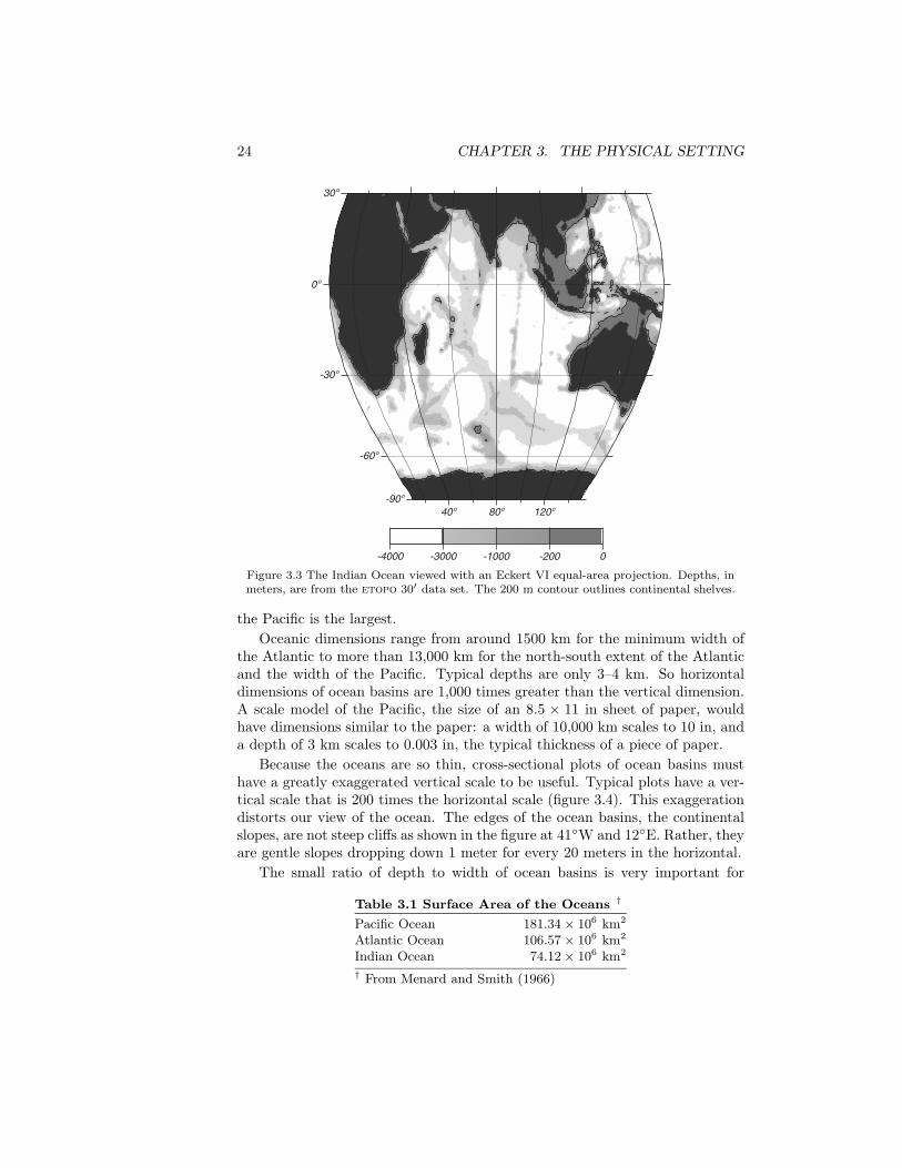
Figure 3.3 The Indian Ocean viewed with an Eckert VI equal-area projection. Depths, inmeters, are from the etopo 30′ data set. The 200 m contour outlines continental shelves.
the Pacific is the largest.Oceanic dimensions range from around 1500 km for the minimum width of
the Atlantic to more than 13,000 km for the north-south extent of the Atlanticand the width of the Pacific. Typical depths are only 3–4 km. So horizontaldimensions of ocean basins are 1,000 times greater than the vertical dimension.A scale model of the Pacific, the size of an 8.5 × 11 in sheet of paper, wouldhave dimensions similar to the paper: a width of 10,000 km scales to 10 in, anda depth of 3 km scales to 0.003 in, the typical thickness of a piece of paper.
Because the oceans are so thin, cross-sectional plots of ocean basins musthave a greatly exaggerated vertical scale to be useful. Typical plots have a ver-tical scale that is 200 times the horizontal scale (figure 3.4). This exaggerationdistorts our view of the ocean. The edges of the ocean basins, the continentalslopes, are not steep cliffs as shown in the figure at 41W and 12E. Rather, theyare gentle slopes dropping down 1 meter for every 20 meters in the horizontal.
The small ratio of depth to width of ocean basins is very important for
Table 3.1 Surface Area of the Oceans †
Pacific Ocean 181.34 × 10⁶ km2
Atlantic Ocean 106.57 × 10⁶ km2
Indian Ocean 74.12 × 10⁶ km2
† From Menard and Smith (1966)

3.3. SEA-FLOOR FEATURES 25D
epth
(km
)
-45o -30o -15o 0o 15o
-6
-4
-2
0
Longitude
6 km6 km
-45o -30o -15o 0o 15o
Figure 3.4 Cross-section of the South Atlantic along 25S showing the continental shelfoffshore of South America, a seamount near 35W, the mid-Atlantic Ridge near 14W, theWalvis Ridge near 6E, and the narrow continental shelf off South Africa. Upper Verticalexaggeration of 180:1. Lower Vertical exaggeration of 30:1. If shown with true aspect ratio,the plot would be the thickness of the line at the sea surface in the lower plot.
understanding ocean currents. Vertical velocities must be much smaller thanhorizontal velocities. Even over distances of a few hundred kilometers, thevertical velocity must be less than 1% of the horizontal velocity. We will usethis information later to simplify the equations of motion.
The relatively small vertical velocities have great influence on turbulence.Three dimensional turbulence is fundamentally different than two-dimensionalturbulence. In two dimensions, vortex lines must always be vertical, and therecan be little vortex stretching. In three dimensions, vortex stretching plays afundamental role in turbulence.
3.3 Sea-Floor FeaturesEarth’s rocky surface is divided into two types: oceanic, with a thin dense crustabout 10 km thick, and continental, with a thick light crust about 40 km thick.The deep, lighter continental crust floats higher on the denser mantle than doesthe oceanic crust, and the mean height of the crust relative to sea level has twodistinct values: continents have a mean elevation of 1100 m, oceans have a meandepth of -3400 m (figure 3.5).
The volume of the water in the oceans exceeds the volume of the oceanbasins, and some water spills over on to the low lying areas of the continents.These shallow seas are the continental shelves. Some, such as the South ChinaSea, are more than 1100 km wide. Most are relatively shallow, with typicaldepths of 50–100 m. A few of the more important shelves are: the East ChinaSea, the Bering Sea, the North Sea, the Grand Banks, the Patagonian Shelf, theArafura Sea and Gulf of Carpentaria, and the Siberian Shelf. The shallow seashelp dissipate tides, they are often areas of high biological productivity, and

26 CHAPTER 3. THE PHYSICAL SETTING
0.0 0.5 1.0 1.5 2.0 2.5 3.0-8
-6
-4
-2
0
2
4
Dep
th (
km)
0 20 40 60 80 100-8
-6
-4
-2
0
2
4
HistogramCumulative
Frequency Curve
Hei
ght (
km)
Figure 3.5 Left Histogram of elevations of land and depth of the sea floor as percentage ofarea of Earth, in 50 m intervals showing the clear distinction between continents and seafloor. Right Cumulative frequency curve of height, the hypsographic curve. The curves arecalculated from the etopo 30′ data set.
they are usually included in the exclusive economic zone of adjacent countries.The crust is broken into large plates that move relative to each other. New
crust is created at the mid-ocean ridges, and old crust is lost at trenches. The
Shore
High Water
Low Water
Sea Level
OCEANSHELF(Gravel,SandAv slope1 in 500)
SLO
PE
(Mudav slope1 in 20)
CO
NT
INE
NT
RISE
BASIN
MID-OCEANRIDGE
DEEP SEA
(Clay & Oozes)Mineral Organic
SE
AM
OU
NT
TR
EN
CH IS
LAN
D A
RC
Figure 3.6 Schematic section through the ocean showing principal features of the sea floor.Note that the slope of the sea floor is greatly exaggerated in the figure.

3.3. SEA-FLOOR FEATURES 27
relative motion of crust, due to plate tectonics, produces the distinctive featuresof the sea floor sketched in figure 3.6, including mid-ocean ridges, trenches,island arcs, and basins. The names of the subsea features have been definedby the International Hydrographic Bureau (1953), and the following definitionsare taken from Sverdrup, Johnson, and Fleming (1942), Shepard (1963), andDietrich et al. (1980).
Basins are deep depressions of the sea floor of more or less circular or ovalform.
Canyons are relatively narrow, deep furrows with steep slopes, cutting acrossthe continental shelf and slope, with bottoms sloping continuously downward.
Continental (or island) shelves are zones adjacent to a continent (or aroundan island) and extending from the low-water line to the depth, usually about120 m, where there is a marked or rather steep descent toward great depths.(figure 3.7)
Continental (or island) slopes are the declivities seaward from the shelf edgeinto greater depth.
Figure 3.7 An example of a continental shelf, the shelf offshore of Monterey Californiashowing the Monterey and other canyons. Canyons are common on shelves, often extendingacross the shelf and down the continental slope to deep water. Figure copyright MontereyBay Aquarium Research Institute (mbari).

28 CHAPTER 3. THE PHYSICAL SETTING
21.4o
21.3o
21.2o
21.1o
21.0o
20.9o
20.8o
163.0o 163.1o 163.2o 163.3o 163.4o 163.5o 163.6o
40
20
14
40
40
2040
48
30
30
Figure 3.8 An example of a seamount, the Wilde Guyot. A guyot is a seamount with a flattop created by wave action when the seamount extended above sea level. As the seamount iscarried by plate motion, it gradually sinks deeper below sea level. The depth was contouredfrom echo sounder data collected along the ship track (thin straight lines) supplementedwith side-scan sonar data. Depths are in units of 100 m. From William Sager, Texas A&MUniversity.
Plains are very flat surfaces found in many deep ocean basins.Ridges are long, narrow elevations of the sea floor with steep sides and rough
topography.Seamounts are isolated or comparatively isolated elevations rising 1000 m or
more from the sea floor and with small summit area (figure 3.8).Sills are the low parts of the ridges separating ocean basins from one another
or from the adjacent sea floor.Trenches are long, narrow, and deep depressions of the sea floor, with rela-
tively steep sides (figure 3.9).Subsea features strongly influences the ocean circulation. Ridges separate
deep waters of the oceans into distinct basins. Water deeper than the sill be-tween two basins cannot move from one to the other. Tens of thousands ofseamounts are scattered throughout the ocean basins. They interrupt oceancurrents, and produce turbulence leading to vertical mixing in the ocean.

3.4. MEASURING THE DEPTH OF THE OCEAN 29
Longitude (West)
Latit
ude
(Nor
th)
-5000
-5000
-5000
-5000
-4000
-4000
-3000
-3000
-2000
-2000
-1000
-1000
-500
-500
-200
-200
-50
-50
-200
0
0
-50
-200
-500
0
-6000
167o 165o 163o 161o 159o 157o 155o51o
52o
53o
54o
55o
56o
57o
51
o 52
o 53 o 54
o 55 o 56
o 57 o
Latitude (North)
-6000
-4000
-2000
0
Dep
th (
m)
Section A:B
A
B
Alaskan Peninsula
Bering Sea
Aleutian Trench
Pacific Ocean
Figure 3.9 An example of a trench, the Aleutian Trench; an island arc, the Alaskan Peninsula;and a continental shelf, the Bering Sea. The island arc is composed of volcanos producedwhen oceanic crust carried deep into a trench melts and rises to the surface. Top: Map ofthe Aleutian region of the North Pacific. Bottom: Cross-section through the region.
3.4 Measuring the Depth of the OceanThe depth of the ocean is usually measured two ways: 1) using acoustic echo-sounders on ships, or 2) using data from satellite altimeters.
Echo Sounders Most maps of the ocean are based on measurements madeby echo sounders. The instrument transmits a burst of 10–30 kHz sound andlistens for the echo from the sea floor. The time interval between transmissionof the pulse and reception of the echo, when multiplied by the velocity of sound,gives twice the depth of the ocean (figure 3.10).
The first transatlantic echo soundings were made by the U.S. Navy DestroyerStewart in 1922. This was quickly followed by the first systematic survey of anocean basin, made by the German research and survey ship Meteor during its

30 CHAPTER 3. THE PHYSICAL SETTING
Transmittertransducer
Receivertransducer
Oscillator
Electromechanicaldrive
Electronics
Bottom
Transmittertransducer
Receivertransducer
Amplifier Oscillator
Time-interval Measurment,
Display, Recording
Strip chart
Surface
Contact bank
Zero-contactswitch
Slidingcontact
Endlessribbon
33 kHzsound pulse
Figure 3.10 Left: Echo sounders measure depth of the ocean by transmitting pulses of soundand observing the time required to receive the echo from the bottom. Right: The time isrecorded by a spark burning a mark on a slowly moving roll of paper. After Dietrich et al.(1980: 124).
expedition to the South Atlantic from 1925 to 1927. Since then, oceanographicand naval ships have operated echo sounders almost continuously while at sea.Millions of miles of ship-track data recorded on paper have been digitized toproduce data bases used to make maps. The tracks are not well distributed.Tracks tend to be far apart in the southern hemisphere, even near Australia(figure 3.11) and closer together in well mapped areas such as the North Atlantic.
Echo sounders make the most accurate measurements of ocean depth. Theiraccuracy is ±1%.
Satellite Altimetry Gaps in our knowledge of ocean depths between shiptracks have now been filled by satellite-altimeter data. Altimeters profile theshape of the sea surface, and it’s shape is very similar to the shape of the seafloor (Tapley and Kim, 2001; Cazenave and Royer, 2001; Sandwell and Smith,2001). To see this, we must first consider how gravity influences sea level.
The Relationship Between Sea Level and the Ocean’s Depth Excess mass atthe sea floor, for example the mass of a seamount, increases local gravity becausethe mass of the seamount is larger than the mass of water it displaces, rocksbeing more than three times denser than water. The excess mass increases localgravity, which attracts water toward the seamount. This changes the shape ofthe sea surface (figure 3.12).
Let’s make the concept more exact. To a very good approximation, the seasurface is a particular level surface called the geoid (see box). By definition alevel surface is everywhere perpendicular to gravity. In particular, it must be

3.4. MEASURING THE DEPTH OF THE OCEAN 31
90o 100o 110o 120o 130o 140o 150o 160o 170o 180o
-40o
-30o
-20o
-10o
0o
Walter H. F. Smith and David T. Sandwell, Ship Tracks, Version 4.0, SIO, September 26, 1996 Copyright 1996, Walter H. F. Smith and David T. Sandwell
Figure 3.11 Locations of echo-sounder data used for mapping the ocean floor near Australia.Note the large areas where depths have not been measured from ships. From David Sandwell,Scripps Institution of Oceanography.
perpendicular to the local vertical determined by a plumb line, which is a linefrom which a weight is suspended. Thus the plumb line is perpendicular tothe local level surface, and it is used to determine the orientation of the levelsurface, especially by surveyors on land.
The excess mass of the seamount attracts the plumb line’s weight, causingthe plumb line to point a little toward the seamount instead of toward Earth’scenter of mass. Because the sea surface must be perpendicular to gravity, it musthave a slight bulge above a seamount as shown in the figure. If there were nobulge, the sea surface would not be perpendicular to gravity. Typical seamountsproduce a bulge that is 1–20 m high over distances of 100–200 kilometers. Ofcourse, this bulge is too small to be seen from a ship, but it is easily measuredby an altimeter. Oceanic trenches have a deficit of mass, and they produce adepression of the sea surface.
The correspondence between the shape of the sea surface and the depth ofthe water is not exact. It depends on the strength of the sea floor and the age ofthe sea-floor feature. If a seamount floats on the sea floor like ice on water, thegravitational signal is much weaker than it would be if the seamount rested onthe sea floor like ice resting on a table top. As a result, the relationship betweengravity and sea-floor topography varies from region to region.
Depths measured by acoustic echo sounders are used to determine the re-gional relationships. Hence, altimetry is used to interpolate between acousticecho sounder measurements. Smith and Sandwell (1994) have used this tech-nique to map the ocean’s depth globally with an accuracy of ±100 m.

32 CHAPTER 3. THE PHYSICAL SETTING
The GeoidThe level surface corresponding to the surface of an ocean at rest is a
special surface, the geoid. To a first approximation, the geoid is an ellipsoidthat corresponds to the surface of a rotating, homogeneous fluid in solid-body rotation, which means that the fluid has no internal flow. To a secondapproximation, the geoid differs from the ellipsoid because of local variationsin gravity. The deviations are called geoid undulations. The maximumamplitude of the undulations is roughly ±60 m. To a third approximation,the geoid deviates from the sea surface because the ocean is not at rest. Thedeviation of sea level from the geoid is defined to be the topography. Thedefinition is identical to the definition for land topography, for example theheights given on a topographic map.
The ocean’s topography is caused by tides and ocean surface currents,and we will return to their influence in chapters 10 and 18. The maximumamplitude of the topography is roughly ±1 m, so it is small compared tothe geoid undulations.
Geoid undulations are caused by local variations in gravity, which aredue to the uneven distribution of mass at the sea floor. Seamounts have anexcess of mass due to their density and they produce an upward bulge inthe geoid (see below). Trenches have a deficiency of mass, and they producea downward deflection of the geoid. Thus the geoid is closely related to sea-floor topography. Maps of the oceanic geoid have a remarkable resemblanceto the sea-floor topography.
sea surface
sea floor
10 m
2 km
200 km
Figure 3.12 Seamounts are more dense than sea water, and they increase local gravitycausing a plumb line at the sea surface (arrows) to be deflected toward the seamount.Because the surface of an ocean at rest must be perpendicular to gravity, the sea surfaceand the local geoid must have a slight bulge as shown. Such bulges are easily measuredby satellite altimeters. As a result, satellite altimeter data can be used to map the seafloor. Note, the bulge at the sea surface is greatly exaggerated, a two-kilometer highseamount would produce a bulge of approximately 10 m.
Satellite-altimeter systems Now let’s see how altimeters can measure theshape of the sea surface. Satellite altimeter systems include a radar to measurethe height of the satellite above the sea surface and a tracking system to deter-

3.5. SEA FLOOR CHARTS AND DATA SETS 33
Satellite's Orbit
Geoid
Geoid Undulation
SeaSurface
Topography(not to scale)Ref
eren
ce
Ellipso
id
Center ofMass
r
h
Figure 3.13 A satellite altimeter measures the height of the satellite above the sea surface.When this is subtracted from the height r of the satellite’s orbit, the difference is sea levelrelative to the center of Earth. The shape of the surface is due to variations in gravity, whichproduce the geoid undulations, and to ocean currents which produce the oceanic topography,the departure of the sea surface from the geoid. The reference ellipsoid is the best smoothapproximation to the geoid. The variations in the geoid, geoid undulations, and topographyare greatly exaggerated in the figure. From Stewart (1985).
mine the height of the satellite in geocentric coordinates. The system measuresthe height of the sea surface relative to the center of mass of Earth (figure 3.13).This gives the shape of the sea surface.
Many altimetric satellites have flown in space. All have had sufficient accu-racy to observe the marine geoid and the influence of sea-floor features on thegeoid. Typical accuracy for the very accurate Topex/Poseidon and Jason satel-lites is ±0.05 m. The most useful satellites include geosat (1985–1988), ers–1(1991–1996), ers–2 (1995– ), Topex/Poseidon (1992–) and Jason (2002–).
Satellite Altimeter Maps of the Sea-floor Topography Seasat, geosat, ers–1, and ers–2 were operated in orbits with ground tracks spaced 3–10 km apart,which was sufficient to map the geoid. The first measurements, which weremade by geosat, were classified by the US Navy, and they were not released toscientists outside the Navy. By 1996 however, the geoid had been mapped bythe Europeans and the Navy released all the geosat data. By combining datafrom all altimetric satellites, Smith and Sandwell reduced the small errors dueto ocean currents and tides, and then produced maps of the geoid and sea floor.
3.5 Sea Floor Charts and Data SetsMost echo-sounder data have been digitized and plotted to make sea-floor charts.Data have been further processed and edited to produce digital data sets whichare widely distributed in cd-rom format. These data have been supplementedwith data from altimetric satellites to produce maps of the sea floor with hori-zontal resolution around 30 km.
The British Oceanographic Data Centre publishes the General BathymetricChart of the Oceans (gebco) Digital Atlas on behalf of the Intergovernmental

34 CHAPTER 3. THE PHYSICAL SETTING
60o
0o
30o
-30o
-60o
180o120o60o -120o -60o 0o Walter H. F. Smith and David T. Sandwell Seafloor Topography Version 4.0 SIO September 26, 1996 © 1996 Walter H. F. Smith and David T. Sandwell
0o
Figure 3.14 The sea-floor topography of the ocean with 3 km resolution produced fromsatellite altimeter observations of the shape of the sea surface. From Smith and Sandwell.
Oceanographic Commission of unesco and the International Hydrographic Bu-reau. The atlas consists primarily of the location of depth contours, coastlines,and tracklines from the gebco 5th Edition published at a scale of 1:10 million.The original contours were drawn by hand based on digitized echo-sounder dataplotted on base maps.
The U.S. National Geophysical Data Center publishes the etopo-5 cd-romcontaining values of digital oceanic depths from echo sounders and land heightsfrom surveys interpolated to a 5-minute (5 nautical mile) grid. Much of thedata were originally compiled by the U.S. Defense Mapping Agency, the U.S.Navy Oceanographic Office, and the U.S. National Ocean Service. Althoughthe map has values on a 5-minute grid, data used to make the map are muchmore sparse, especially in the southern ocean, where distances between shiptracks can exceed 500 km in some regions (figure 3.11). The same data set andcd-rom contains values smoothed and interpolated to a 30-minute grid.
Sandwell and Smith of the Scripps Institution of Oceanography distribute adigital sea-floor atlas of the oceans based on measurements of the height of thesea surface made from geosat and ers–1 altimeters and echo-sounder data.This map has a horizontal resolution of 30 km and a vertical accuracy of ±100m (Smith and Sandwell, 1997). The US National Geophysical Data Centercombined the Sandwell and Smith data with land elevations to produce a globalmap with 2-minute horizontal resolution. These maps show much more detailthan the etopo-5 map because the satellite data fill in the regions between shiptracks (figure 3.14).
National governments publish coastal and harbor maps. In the USA, thenoaa National Ocean Service publishes nautical charts useful for navigation ofships in harbors and offshore waters.

3.6. SOUND IN THE OCEAN 35
3.6 Sound in the OceanSound provides the only convenient means for transmitting information overgreat distances in the ocean, and it is the only signal that can be used for theremotely sensing of the ocean below a depth of a few tens of meters. Sound isused to measure the properties of the sea floor, the depth of the ocean, tem-perature, and currents. Whales and other ocean animals use sound to navigate,communicate over great distances, and find food.
Sound Speed The sound speed in the ocean varies with temperature, salinity,and pressure (MacKenzie, 1981; Munk et al. 1995: 33):
C = 1448.96 + 4.591 t − 0.05304 t2 + 0.0002374 t3 + 0.0160 Z (3.1)
+ (1.340 − 0.01025 t)(S − 35) + 1.675 × 10⁻⁷ Z − 7.139 × 10⁻¹³ t Z3
where C is speed in m/s, t is temperature in Celsius, S is salinity in practicalsalinity units (see Chapter 6 for a definition of salinity), and Z is depth in meters.The equation has an accuracy of about 0.1 m/s (Dushaw et al. 1993). Othersound-speed equations have been widely used, especially an equation proposedby Wilson (1960) which has been widely used by the U.S. Navy.
For typical oceanic conditions, C is usually between 1450 m/s and 1550 m/s(figure 3.15). Using (3.1), we can calculate the sensitivity of C to changes oftemperature, depth, and salinity typical of the ocean. The approximate valuesare: 40 m/s per 10C rise of temperature, 16 m/s per 1000 m increase in depth,and 1.5 m/s per 1 psu increase in salinity. Thus the primary causes of variabilityof sound speed is temperature and depth (pressure). Variations of salinity aretoo small to have much influence.
If we plot sound speed as a function of depth, we find that the speed usuallyhas a minimum at a depth around 1000 m (figure 3.16). The depth of minimumspeed is called the sound channel . It occurs in all oceans, and it usually reachesthe surface at very high latitudes.
The sound channel is really important because sound in the channel cantravel very far, sometimes half way around the earth. Here is how the channelworks. Sound rays that begin to travel out of the channel are refracted backtoward the center of the channel. Rays propagating upward at small anglesto the horizontal are bent downward, and rays propagating downward at smallangles to the horizontal are bent upward (figure 3.16). Typical depths of thechannel vary from 10 m to 1200 m depending on geographical area.
Absorption of Sound Absorption of sound per unit distance depends on theintensity I of the sound:
dI = −kI0 dx (3.2)
where I0 is the intensity before absorption and k is an absorption coefficientwhich depends on frequency of the sound. The equation has the solution:
I = I0 exp(−kx) (3.3)

36 CHAPTER 3. THE PHYSICAL SETTING
S (psu)
0 o 5
o 10 o 15
o 20 o
-6
-5
-4
-3
-2
-1
0
Dep
th (
km)
33.0 33.5 34.0 34.5 35.0
Speed Corrections (m/s)
0 20 40 60 80 100
0 20 40 60 80 100
Sound Speed (m/s)
1500 1520 1540 1560
1500 1520 1540 1560
-6
-5
-4
-3
-2
-1
-0
t S
C
T oC
∆Ct ∆CP ∆CS
Figure 3.15 Processes producing the sound channel in the ocean. Left: Temperature T andsalinity S measured as a function of depth during the R.V. Hakuho Maru cruise KH-87-1,station JT, on 28 January 1987 at Latitude 3352.90′ N, Long 14155.80′ E in the NorthPacific. Center: Variations in sound speed due to variations in temperature, salinity, anddepth. Right: Sound speed as a function of depth showing the velocity minimum near 1km depth which defines the sound channel in the ocean. (Data from jpots Editorial Panel,1991).
Typical values of k (in decibels dB per kilometer) are: 0.08 dB/km at 1000 Hz,and 50 dB/km at 100,000 Hz. Decibels are calculated from: dB = 10 log(I/I0).where I0 is the original acoustic power, I is the acoustic power after absorption.
For example, at a range of 1 km a 1000 Hz signal is attenuated by only 1.8%:I = 0.982I0. At a range of 1 km a 100,000 Hz signal is reduced to I = 10−5I0.In particular the 30,000 Hz signal used by typical echo sounders to map theocean’s depth are little attenuated going from the surface to the bottom andback.
Very low frequency sounds in the sound channel, those with frequenciesbelow 500 Hz have been detected at distances of megameters. In 1960 15-Hzsounds from explosions set off in the sound channel off Perth Australia wereheard in the sound channel near Bermuda, nearly halfway around the world.Later experiment showed that 57-Hz signals transmitted in the sound channelnear Heard Island (75E, 53S) could be heard at Bermuda in the Atlantic andat Monterey, California in the Pacific (Munk et al. 1994).
Use of Sound Because low frequency sound can be heard at great distances,the US Navy, in the 1950s, placed arrays of microphones on the sea floor indeep and shallow water and connected them to shore stations. The Sound

3.7. IMPORTANT CONCEPTS 37
+9+10
-9
ray +8
Range (km)
0 100 2001.50 1.55
-0
-1
-2
-3
-4
Dep
th (
km
)
C (km/s)
axis
Figure 3.16 Ray paths of sound in the ocean for a source nearthe axis of the sound channel. After Munk et al. (1995).
Surveillance System sosus, although designed to track submarines, has foundmany other uses. It has been used to listen to and track whales up to 1,700 kmaway, and to find the location of subsea volcanic eruptions.
3.7 Important Concepts1. If the oceans were scaled down to a width of 8 inches they would have
depths about the same as the thickness of a piece of paper. As a result,the velocity field in the ocean is nearly 2-dimensional. Vertical velocitiesare much smaller than horizontal velocities.
2. There are only three official oceans.
3. The volume of ocean water exceeds the capacity of the ocean basins, andthe oceans overflow on to the continents creating continental shelves.
4. The depths of the ocean are mapped by echo sounders which measure thetime required for a sound pulse to travel from the surface to the bottomand back. Depths measured by ship-based echo sounders have been used toproduce maps of the sea floor. The maps have poor horizontal resolutionin some regions because the regions were seldom visited by ships and shiptracks are far apart.
5. The depths of the ocean are also measured by satellite altimeter systemswhich profile the shape of the sea surface. The local shape of the surfaceis influenced by changes in gravity due to subsea features. Recent mapsbased on satellite altimeter measurements of the shape of the sea surfacecombined with ship data have depth accuracy of ±100 m and horizontalresolutions of ±3 km.
6. Typical sound speed in the ocean is 1480 m/s. Speed depends primarilyon temperature, less on pressure, and very little on salinity. The variabil-ity of sound speed as a function of pressure and temperature produces a

38 CHAPTER 3. THE PHYSICAL SETTING
horizontal sound channel in the ocean. Sound in the channel can travelgreat distances. Low-frequency sounds below 500 Hz can travel halfwayaround the world provided the path is not interrupted by land.

Chapter 4
Atmospheric Influences
The sun and the atmosphere drive directly or indirectly almost all dynamicalprocesses in the ocean. The dominant external sources and sinks of energyare sunlight, evaporation, infrared emissions from the sea surface, and sensibleheating of the sea by warm or cold winds. Winds drive the ocean’s surfacecirculation down to depths of around a kilometer. Wind and tidal mixing drivethe deeper currents in the ocean.
The oceans, in turn, help drive the atmospheric circulation. The unevendistribution of heat loss and gain by the ocean leads to winds in the atmosphere.Sunlight warms the tropical oceans, which evaporate, transferring heat in theform of moisture to the atmosphere. Winds and ocean currents carry heatpoleward, where it is lost to space.
Because the atmosphere helps drive the ocean, and the ocean helps drivethe atmosphere, we must consider the ocean and the atmosphere as a coupleddynamic system. In this chapter we will look at the exchange of heat and waterbetween the atmosphere and the ocean. Later, we will explore the influence ofthe wind on the ocean and the exchange of momentum leading to wind-drivenocean currents. Then we will look at how the ocean and the atmosphere interactin the Pacific to produce El Nino.
4.1 The Earth in SpaceThe Earth’s orbit about the sun is nearly circular at a mean distance of 1.5×10⁸
km. The eccentricity of the orbit is small, 0.0168. Thus Earth is 103.4% furtherfrom the Sun at aphelion than at perihelion, the time of closest approach to thesun. Perihelion occurs every year in January, and the exact time changes byabout 20 minutes per year. In 1995, it occurred on 3 January. Earth’s axis ofrotation is inclined 23.45 to the plane of earth’s orbit around the sun (figure4.1). The orientation is such that the sun is directly overhead at the Equatoron the vernal and autumnal equinoxes, which occur on or about 21 March and21 September each year.
The latitudes of 23.45 North and South are the Tropics of Cancer andCapricorn respectively. The tropics lie equatorward of these latitudes. As a
39

40 CHAPTER 4. ATMOSPHERIC INFLUENCES
Sun
Tropic ofCapricorn
Wintersolstice
Arctic CircleAutumnalequinox
Antarctic Circle
Vernal equinox
Tropic ofCancer
Summersolstice
23 12o
Figure 4.1 The Earth in space. The ellipticity of Earth’s orbit around the sun and the tilt ofEarth’s axis of rotation relative to the plane of Earth orbit leads to an unequal distributionof heating and to the seasons.
result of the eccentricity of earth’s orbit, maximum solar insolation averagedover the surface of the earth occurs in early January each year. As a resultof the inclination of earth’s axis of rotation, the maximum insolation at anylocation outside the tropics occurs around 21 June in the northern hemisphere,and around 21 December in the southern hemisphere.
Annual Wind Speed and Sea Level Pressure (hPa) For 1989
1012 1012 10141014
1014 1014 10
14
1012
1014
1014
1014
1014
1014
1014 1014
1012
1012
1012
1012
1012
1018
1018
1018
1012
1018
1018
1018
10121014
1018
1018
1000
990990
10001000
1010 1010
1010
1010
1010
1010
1010
1020
980
1010
1020
1010
1020
980
1010
1020
1020
1010
1012
1014
1012
1010
990 990
990
20o 60o 100o 140o 180o -140o -100o -60o -20o 20o-90o
-60o
-30o
0o
30o
60o
90o
0o
Figure 4.2 Map of mean annual wind velocity calculated from Trenberth et al. (1990) andsea-level pressure for 1989 from the nasa Goddard Space Flight Center’s Data AssimilationOffice (Schubert et al. 1993). The winds near 140W in the equatorial Pacific are about 8m/s.

4.2. ATMOSPHERIC WIND SYSTEMS 41
If solar heat was rapidly redistributed over Earth, maximum temperaturewould occur in January. Conversely, if heat were poorly redistributed, maximumtemperature in the northern hemisphere would occur in summer. So it is clearthat heat is not rapidly redistributed by winds and currents.
4.2 Atmospheric Wind SystemsFigure 4.2 shows the distribution of sea-level winds and pressure averaged overthe year 1989. The map shows strong winds from the west between 40 to 60
latitude, the roaring forties, weak winds in the subtropics near 30 latitude,trade winds from the east in the tropics, and weaker winds from the east alongthe Equator. The strength and direction of winds in the atmosphere is theresult of uneven distribution of solar heating and continental land masses andthe circulation of winds in a vertical plane in the atmosphere.
A simple cartoon of the distribution of winds in the atmosphere (figure 4.3)
Equatorial Low or Doldrums
Subtropical High or Horse latitudes
Subpolar Low
Polar High
Subpolar Low
Subtropical High or Horse latitudes
Polar High
easterlies
westerlies
North-East Trades
South-East Trades
westerlies
easterlies
60o
-60o -60o
-30o-30o
30o30o
0o0o
-90o
90o
heavy precipitation
variable winds and calms
large evaporation
variable winds and calms
very heavy precipitation variable winds and calms
large evaporation
sinking air
risingairupper westerlies
sinking air
rising air
Had
ley
c
ells
upper westerlies
sinking air
risingair
sinking air
heavy precipitation
60o
moist air
10
20
0Pole easterlies 60o westerlies 30o Trade Winds
PolarHigh
SubpolarLow
SubpolarHigh
IntertropicalConvergence Zone
EquatorialLow
troposphere
polar
front
tropopause
temperature inversioncumulonimbus
activityPOLARPOLAR
SUBSUBTROPICALTROPICAL
Hei
ght (
km)
Figure 4.3 Sketch of Earth’s atmospheric circulation driven by solar heating in the tropicsand cooling at high latitudes. Upper: The meridional cells in the atmosphere and theinfluence of Earth’s rotation on the winds. Bottom: Cross-section through the atmosphereshowing the two major cells of meridional circulation. After The Open University (1989a:14).

42 CHAPTER 4. ATMOSPHERIC INFLUENCES
shows that the surface winds are influenced by equatorial convection and otherprocesses higher in the atmosphere. The mean value of winds over the ocean is(Wentz et al. 1984):
U10 = 7.4 m/s (4.1)
Maps of surface winds change somewhat with the seasons. The largestchanges are in the Indian Ocean and the western Pacific Ocean (figure 4.4).Both regions are strongly influenced by the Asian monsoon. In winter, the coldair mass over Siberia creates a region of high pressure at the surface, and cold
July Wind Speed
January Wind Speed
20o 60o 100o 140o 180o -140o -100o -60o -20o 20o-90o
-60o
-30o
0o
30o
60o
90o
0o
20o 60o 100o 140o 180o -140o -100o -60o -20o 20o-90o
-60o
-30o
0o
30o
60o
90o
0o
Figure 4.4 Mean, sea-surface winds for July and January calculated from the Trenberth et al.(1990) data set, which is based on the ecmwf reanalyses of weather data from 1980 to 1989.The winds near 140W in the equatorial Pacific are about 8 m/s.
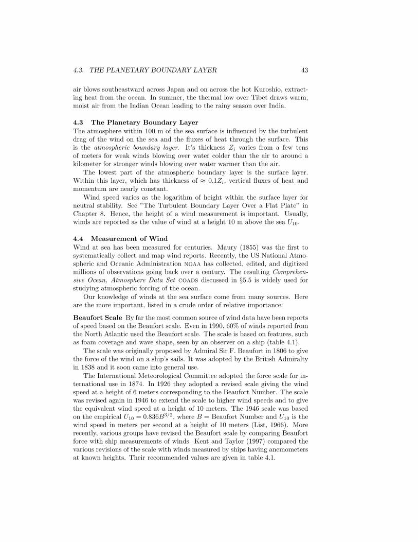
4.3. THE PLANETARY BOUNDARY LAYER 43
air blows southeastward across Japan and on across the hot Kuroshio, extract-ing heat from the ocean. In summer, the thermal low over Tibet draws warm,moist air from the Indian Ocean leading to the rainy season over India.
4.3 The Planetary Boundary LayerThe atmosphere within 100 m of the sea surface is influenced by the turbulentdrag of the wind on the sea and the fluxes of heat through the surface. Thisis the atmospheric boundary layer. It’s thickness Zi varies from a few tensof meters for weak winds blowing over water colder than the air to around akilometer for stronger winds blowing over water warmer than the air.
The lowest part of the atmospheric boundary layer is the surface layer.Within this layer, which has thickness of ≈ 0.1Zi, vertical fluxes of heat andmomentum are nearly constant.
Wind speed varies as the logarithm of height within the surface layer forneutral stability. See ”The Turbulent Boundary Layer Over a Flat Plate” inChapter 8. Hence, the height of a wind measurement is important. Usually,winds are reported as the value of wind at a height 10 m above the sea U10.
4.4 Measurement of WindWind at sea has been measured for centuries. Maury (1855) was the first tosystematically collect and map wind reports. Recently, the US National Atmo-spheric and Oceanic Administration noaa has collected, edited, and digitizedmillions of observations going back over a century. The resulting Comprehen-sive Ocean, Atmosphere Data Set coads discussed in §5.5 is widely used forstudying atmospheric forcing of the ocean.
Our knowledge of winds at the sea surface come from many sources. Hereare the more important, listed in a crude order of relative importance:
Beaufort Scale By far the most common source of wind data have been reportsof speed based on the Beaufort scale. Even in 1990, 60% of winds reported fromthe North Atlantic used the Beaufort scale. The scale is based on features, suchas foam coverage and wave shape, seen by an observer on a ship (table 4.1).
The scale was originally proposed by Admiral Sir F. Beaufort in 1806 to givethe force of the wind on a ship’s sails. It was adopted by the British Admiraltyin 1838 and it soon came into general use.
The International Meteorological Committee adopted the force scale for in-ternational use in 1874. In 1926 they adopted a revised scale giving the windspeed at a height of 6 meters corresponding to the Beaufort Number. The scalewas revised again in 1946 to extend the scale to higher wind speeds and to givethe equivalent wind speed at a height of 10 meters. The 1946 scale was basedon the empirical U10 = 0.836B3/2, where B = Beaufort Number and U10 is thewind speed in meters per second at a height of 10 meters (List, 1966). Morerecently, various groups have revised the Beaufort scale by comparing Beaufortforce with ship measurements of winds. Kent and Taylor (1997) compared thevarious revisions of the scale with winds measured by ships having anemometersat known heights. Their recommended values are given in table 4.1.

44 CHAPTER 4. ATMOSPHERIC INFLUENCES
Table 4.1 Beaufort Wind Scale and State of the Sea
Beaufort Descriptive m/s Appearance of the SeaNumber term
0 Calm 0 Sea like a mirror.1 Light Air 1.2 Ripples with appearance of scales; no foam crests.2 Light Breeze 2.8 Small wavelets; crests of glassy appearance,
not breaking.3 Gentle breeze 4.9 Large wavelets; crests begin to break; scattered
whitecaps.4 Moderate breeze 7.7 Small waves, becoming longer; numerous whitecaps.5 Fresh breeze 10.5 Moderate waves, taking longer to form; many
whitecaps; some spray.6 Strong breeze 13.1 Large waves forming; whitecaps everywhere;
more spray.7 Near gale 15.8 Sea heaps up; white foam from breaking waves begins
to be blown into streaks.8 Gale 18.8 Moderately high waves of greater length; edges of
crests begin to break into spindrift; foam is blownin well-marked streaks.
9 Strong gale 22.1 High waves; sea begins to roll; dense streaks of foam;spray may reduce visibility.
10 Storm 25.9 Very high waves with overhanging crests; sea takeswhite appearance as foam is blown in very densestreaks; rolling is heavy and visibility reduced.
11 Violent storm 30.2 Exceptionally high waves; sea covered with whitefoam patches; visibility still more reduced.
12 Hurricane 35.2 Air is filled with foam; sea completely whitewith driving spray; visibility greatly reduced.
From Kent and Taylor (1997)
Observers on ships everywhere in the world usually report weather observa-tions, including Beaufort force, at the same four times every day. The times areat 0000Z, 0600Z, 1200Z and 1800Z, where Z indicates Greenwich Mean Time.The reports are coded and reported by radio to national meteorological agen-cies. The biggest error in the reports is the sampling error. Ships are unevenlydistributed over the ocean. They tend to avoid high latitudes in winter andhurricanes in summer, and few ships cross the southern hemisphere (figure 4.5).Overall, the accuracy is around 10%.
Scatterometers Observations of winds at sea now come mostly from scat-terometers on satellites (Liu, 2002). The scatterometer is a instrument verymuch like a radar that measures the scatter of centimeter-wavelength radiowaves from small, centimeter-wavelength waves on the sea surface. The area ofthe sea covered by small waves, and their amplitude depends on wind speed anddirection. The scatterometer measures scatter from 2–4 directions, from whichwind speed and direction are calculated.
The scatterometers on ers-1 and 2 have made global measurements of windsfrom space since 1991. The nasa scatterometer on adeos measured winds for asix-month period beginning November 1996 and ending with the premature fail-ure of the satellite. It was replaced by the Seawinds scatterometers on Quikscat,launched in 1999, and on Midori-2, launched in early 2003. Seawinds views 93%
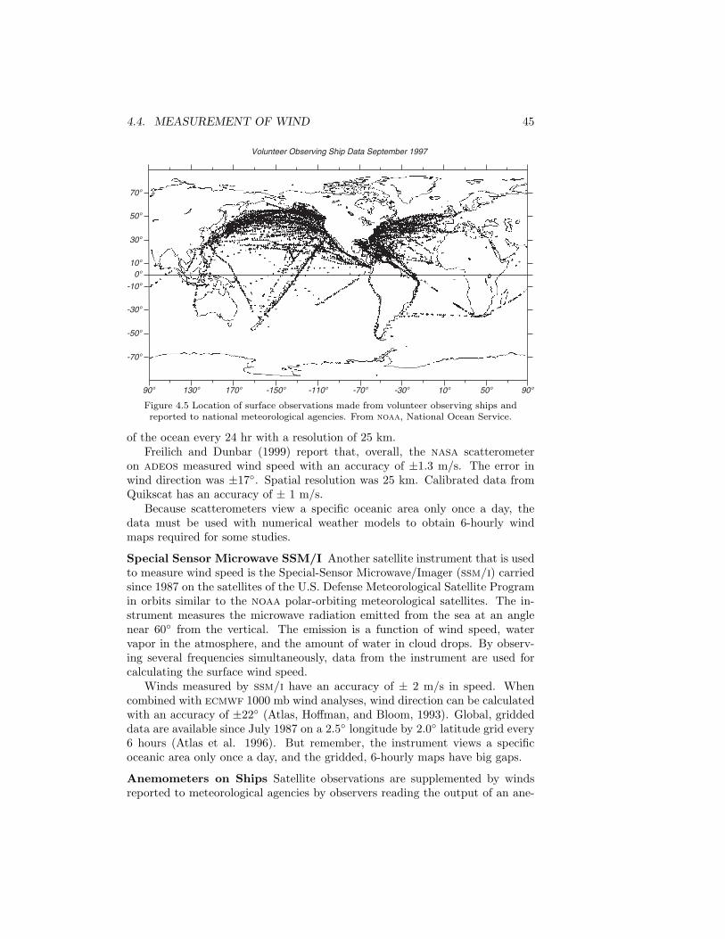
4.4. MEASUREMENT OF WIND 45
Volunteer Observing Ship Data September 1997
90o 130o 170o -150o -110o -70o -30o 10o 50o
10o
-10o
-30o
-50o
-70o
30o
50o
70o
90o
0o
Figure 4.5 Location of surface observations made from volunteer observing ships andreported to national meteorological agencies. From noaa, National Ocean Service.
of the ocean every 24 hr with a resolution of 25 km.Freilich and Dunbar (1999) report that, overall, the nasa scatterometer
on adeos measured wind speed with an accuracy of ±1.3 m/s. The error inwind direction was ±17. Spatial resolution was 25 km. Calibrated data fromQuikscat has an accuracy of ± 1 m/s.
Because scatterometers view a specific oceanic area only once a day, thedata must be used with numerical weather models to obtain 6-hourly windmaps required for some studies.
Special Sensor Microwave SSM/I Another satellite instrument that is usedto measure wind speed is the Special-Sensor Microwave/Imager (ssm/i) carriedsince 1987 on the satellites of the U.S. Defense Meteorological Satellite Programin orbits similar to the noaa polar-orbiting meteorological satellites. The in-strument measures the microwave radiation emitted from the sea at an anglenear 60 from the vertical. The emission is a function of wind speed, watervapor in the atmosphere, and the amount of water in cloud drops. By observ-ing several frequencies simultaneously, data from the instrument are used forcalculating the surface wind speed.
Winds measured by ssm/i have an accuracy of ± 2 m/s in speed. Whencombined with ecmwf 1000 mb wind analyses, wind direction can be calculatedwith an accuracy of ±22 (Atlas, Hoffman, and Bloom, 1993). Global, griddeddata are available since July 1987 on a 2.5 longitude by 2.0 latitude grid every6 hours (Atlas et al. 1996). But remember, the instrument views a specificoceanic area only once a day, and the gridded, 6-hourly maps have big gaps.
Anemometers on Ships Satellite observations are supplemented by windsreported to meteorological agencies by observers reading the output of an ane-

46 CHAPTER 4. ATMOSPHERIC INFLUENCES
mometers on ships. The output of the anemometer is read four times a day atthe standard Greenwich times and reported via radio to meteorological agencies.
Again, the biggest error is the sampling error. Very few ships carry calibratedanemometers. Those that do tend to be commercial ships participating in theVolunteer Observing Ship program. These ships are met in port by scientistswho check the instruments and replace them if necessary, and who collect thedata measured at sea. The accuracy of wind measurements from these ships isabout ±2 m/s.
Calibrated Anemometers on Weather Buoys The most accurate measure-ments of winds at sea are made by calibrated anemometers on moored weatherbuoys. Unfortunately there are few such buoys, perhaps only a hundred scat-tered around the world. Some, such as Tropical Atmosphere Ocean tao arrayin the tropical Pacific (figure 14.14) provide data from remote areas rarely vis-ited by ships, but most tend to be located just offshore of coastal areas. noaaoperates buoys offshore of the United States and the tao array in the Pacific.Data from the coastal buoys are averaged for eight minutes before the hour, andthe observations are transmitted to shore via satellite links.
The best accuracy of anemometers on buoys operated by the us NationalData Buoy Center is the greater of ±1 m/s or 10% for wind speed and ±10 forwind direction (Beardsley et al. 1997).
4.5 Calculations of WindSatellites, ships, and buoys measure winds at various locations and times of theday. If you wish to use the observations to calculate monthly averaged windsover the sea, then the observations can be averaged and gridded. If you wish touse wind data in numerical models of the ocean’s currents, then the data willbe less useful. You are faced with a very common problem: How to take allobservations made in a six-hour period and determine the winds over the oceanon say a fixed grid?
One source of gridded winds over the ocean is the output from numericalweather models. The strategy used to produce the six-hourly gridded winds iscalled sequential estimation techniques or data assimilation. “Measurements areused to prepare initial conditions for the model, which is then integrated forwardin time until further measurements are available. The model is thereupon re-initialized” (Bennett, 1992: 67).
Usually, all available measurements are used, including observations fromweather stations on land, pressure and temperature reported by ships and buoys,winds from scatterometers in space, and data from meteorological satellites. Themodel interpolates the measurements to produce the initial conditions consistentwith previous and present observations. Daley (1991) describes the techniquesin considerable detail.
Surface Analysis from Numerical Weather Models Perhaps the mostwidely used weather model is that run by the European Centre for Medium-range Weather Forecasts ecmwf. It calculates surface winds and heat fluxes

4.5. CALCULATIONS OF WIND 47
(see Chapter 5) every six hours on a 1 × 1 grid from an explicit boundary-layermodel. Calculated values are archived on a 2.5grid. Thus the wind maps fromthe numerical weather models lack the detail seen in maps from scatterometerdata, which have a 1/4/degrees grid.
ecmwf calculations of winds have relatively good accuracy. Freilich andDunbar (1999) estimated that the accuracy for wind speed at 10 meters is ±1.5m/s, and ±18 for direction.
Accuracy in the southern hemisphere is probably as good as in the northernhemisphere because continents do not disrupt the flow as much as in the northernhemisphere, and because scatterometers give accurate positions of storms andfronts over the ocean.
Other surface-analysis values used in oceanography include: 1) output fromthe numerical weather model run by the noaa National Centers for Environ-mental Prediction, 2) the Planetary Boundary-Layer Data set produced by theU.S. Navy’s Fleet Numerical Oceanography Center fnoc, and 3) surface windmaps for the tropics produced at Florida State University (Goldenberg andO’Brien, 1981).
Reanalyzed Output from Numerical Weather Models The output fromnumerical models of the atmospheric circulation has been available for decades.Throughout this period, the models have been constantly changed as meteorol-ogists strive to make ever more accurate forecasts. Fluxes calculated from themodels are therefore not consistent in time. The changes can be larger than theinterannual variability of the fluxes (White, 1996). To minimize this problem,meteorological agencies have taken all archived weather data and reanalyzedthem using the best numerical models now available to produce a uniform,internally-consistent, surface analysis.
The reanalyzed data sets are now being used to study oceanic and atmo-spheric dynamics. The surface analysis data sets are used only for problems thatrequire up-to-date information. For example, if you are designing an offshorestructure, you will probably use decades of reanalyzed data. If you are operat-ing an offshore structure, you will watch the surface analysis and forecasts putout every six hours by meteorological agencies.
Sources of Reanalyzed Data Reanalyzed surface flux data are available fromnational meteorological centers operating numerical weather prediction models.
1. The U.S. National Centers for Environmental Predictions, working withthe National Center for Atmospheric Research have produced the ncep/ncar reanalysis based on 51 years of weather data from 1948 to 1998 usingthe 25 January 1995 version of their forecast model. The reanalysis periodwill be extended forward to include all date up to the present with abouta three-day delay in producing data sets. The reanalysis uses surface andship observations plus sounder data from satellites. Reanalyzed productsare available every six hours on a T62 grid having 192 × 94 grid pointswith a spatial resolution of 209 km and with 28 vertical levels. Importantsubsets of the reanalyzed data, including surface fluxes, are available oncd–rom (Kalnay et al. 1996; Kistler et al. 2000).

48 CHAPTER 4. ATMOSPHERIC INFLUENCES
2. The European Centre for Medium-range Weather Forecasts ecmwf hasreanalyzed 17 years of weather data from 1979 to 1993. The reanalysis usesmostly the same surface, ship and satellite data used by the ncep/ncarreanalysis. The European Centre is extending the reanalysis to cover a40-year period from 1957–1997. Spatial resolution will be 83 km, temporalresolution will be 6 hours. The reanalysis will use most available satellitedata sets, including data from the ers-1 and ers-2 satellites and ssm/i.The analysis will include an ocean-wave model and it will calculate oceanwave heights.
3. The Data Assimilation Office at nasa’s Goddard Earth Observing Systemhas completed a reanalysis for the period 1 March 1980 to 13 December1993 later extended to February 1995. The analyzed data are availableevery six hours on a 2×2.5(91 × 144 point) grid with 20 vertical levels.The analysis uses the ncep real-time in-situ observations plus tovs datafrom the noaa meteorological satellites and cloud-drift winds (Schubert,Rood, and Pfaendtner, 1993). The analysis places special emphasis on theassimilation of satellite data using the Goddard Earth Observing Systemnumerical weather model.
4.6 Wind StressThe wind, by itself, is usually not very interesting. Often we are much moreinterested in the force of the wind, or the work done by the wind. The horizontalforce of the wind on the sea surface is called the wind stress. Put another way, itis the vertical transfer of horizontal momentum. Thus momentum is transferredfrom the atmosphere to the ocean by wind stress.
Wind stress T is calculated from:
T = ρ CDU210 (4.2)
where ρ = 1.3 kg/m3 is the density of air, U10 is wind speed at 10 meters, andCD is the drag coefficient . CD is measured using the techniques described in§5.6. Fast response instruments measure wind fluctuations within 10–20 m ofthe sea surface, from which T is directly calculated. The correlation of T withU2
10 gives CD (figure 4.6).Various measurements of CD have been published based on careful measure-
ments of turbulence in the marine boundary layer. Trenberth et al. (1989)and Harrison (1989) discuss the accuracy of an effective drag coefficient relatingwind stress to wind velocity on a global scale. Perhaps the most recently pub-lished values are those of Yelland and Taylor (1996) and Yelland et al. (1998)who give:
1000 CD = 0.29 +3.1U10
+7.7U2
10
(3 ≤ U10 ≤ 6 m/s) (4.3a)
1000 CD = 0.50 + 0.071 U10 (6 ≤ U10 ≤ 26 m/s) (4.3b)

4.7. IMPORTANT CONCEPTS 49
0
0.001
0.002
0.003
CD
U10 (m/s)
5 10 15 200 30 35 40 4525 5550
Figure 4.6 The drag coefficient as a function of wind speed U10 ten meters above the sea.Circles: Measured values from Smith (1980). Triangles: Measured values from Powell,Vickery, and Reinhold (2003). The solid line is from eq (4.3) proposed by Yelland and Taylor(1996).
for neutrally stable boundary layer. Other values are listed in their table 1 andin figure 4.6.
Useful monthly maps of oceanic wind stress suitable for studies of the oceancirculation have been published by Trenberth et al. (1990) who used analyzedwind fields from ecmwf to produce maps with 2.5 resolution.
4.7 Important Concepts1. Sunlight is the primary energy source driving the atmosphere and oceans.
2. There is a boundary layer at the bottom of the atmosphere where windspeed decreases with as the boundary is approached, and in which fluxesof heat and momentum are constant in the lower 10–20 meters.
3. Wind is measured many different ways. The most common until 1995 wasfrom observations made at sea of the Beaufort force of the wind.
4. Since 1995, the most important source of wind measurements is fromscatterometers on satellites. They produce daily global maps with 25km resolution.
5. The output from numerical models of the atmosphere is the most usefulsource of global, gridded maps of wind velocity for dates before 1995. Italso is a useful source for 6-hourly maps. Resolution is 100-250 km.
6. The flux of momentum from the atmosphere to the ocean, the wind stress,is calculated from wind speed using a drag coefficient.

50 CHAPTER 4. ATMOSPHERIC INFLUENCES

Chapter 5
The Oceanic Heat Budget
About half the sunlight reaching Earth is absorbed by the oceans and land,where it is temporarily stored near the surface. Only about a fifth of the avail-able sunlight is directly absorbed by the atmosphere. Of the heat stored by theocean, part is released locally to the atmosphere, mostly by evaporation andinfrared radiation. The remainder is transported by currents to other areas es-pecially mid latitudes. Solar radiation stored in the ocean is therefore availableto ameliorate Earth’s climate. The transport of heat is not steady, and sig-nificant changes in heat transport, particularly in the Atlantic, may have beenimportant for the development of the ice ages. For these reasons, oceanic heatbudgets and transports are important for understanding Earth’s climate and itsshort and long term variability.
5.1 The Oceanic Heat BudgetChanges in heat stored in the upper layers of the ocean result from a localimbalance between input and output of heat through the sea surface. Thistransfer of heat across or through a surface is called a heat flux . The flux ofheat to deeper layers is usually much smaller than the flux through the surface.Heat carried out of the area by currents, called advection, will be describedlater. Globally, the sum of all the heat fluxes into and out of the ocean must bezero, otherwise the oceans as a whole would heat up or cool down.
The sum of the heat fluxes into or out of a volume of water is the heat budget.The major terms in the budget at the sea surface are:
1. Insolation QSW , the flux of sunlight into the sea;2. Net Infrared Radiation QLW , net flux of infrared radiation from the sea;3. Sensible Heat Flux QS , the flux of heat out of the sea due to conduction;4. Latent Heat Flux QL, the flux of heat carried by evaporated water; and5. Advection QV , heat carried away by currents.
Conservation of heat requires:
Q = QSW + QLW + QS + QL + QV (5.1)
51

52 CHAPTER 5. THE OCEANIC HEAT BUDGET
4.004.054.104.15
4.20
0o
10o
20o
30o
Tem
pera
ture
(C
elsi
us)
0 10 20 30 40
Salinity
Figure 5.1 Specific heat of sea water at atmospheric pressure Cp in joules per gram per degreeCelsius as a function of temperature in Celsius and salinity, calculated from the empiricalformula given by Millero et al. (1973) using algorithms in Fofonoff and Millard (1983). Thelower line is the freezing point of salt water.
where Q is the resultant heat gain or loss. Units for heat fluxes are watts/m2.The product of flux times surface area times time is energy in joules. The changein temperature ∆t of the water is related to change in energy ∆E through:
∆E = Cp m ∆t (5.2)
where m is the mass of water being warmed or cooled, and Cp is the specificheat of sea water at constant pressure.
Cp ≈ 4.0 × 10³ J · kg−1 · C−1 (5.3)
Thus, 4,000 joules of energy are required to heat 1.0 kilogram of sea water by1.0C (figure 5.1).
Importance of the Ocean in Earth’s Heat Budget To understand theimportance of the ocean in Earth’s heat budget, let’s make a simple comparisonof the heat stored in the ocean with heat stored on land during an annual cycle.During the cycle, heat is stored in summer and released in the winter. The pointis to show that the oceans store and release much more heat than the land.
To begin, we use (5.3) and the heat capacity of soil and rocks
Cp(rock) = 800 J · kg−1 · C−1 (5.4)
to obtain Cp(rock) ≈ 0.2 Cp(water).The volume of water which exchanges heat with the atmosphere on a seasonal
cycle is 100 m3 per square meter of surface, i.e. that mass from the surface toa depth of 100 meters. The density of water is 1000 kg/m3, and the mass in

5.2. HEAT-BUDGET TERMS 53
contact with the atmosphere is density × volume = mwater = 100, 000 kg. Thevolume of land which exchanges heat with the atmosphere on a seasonal cycleis 1 m3. Because the density of rock is 3,000 kg/m3, the mass of the soil androck in contact with the atmosphere is 3,000 kg.
The seasonal heat storage values for the ocean and land are therefore:
∆Eoceans = Cp(water) mwater ∆t ∆t = 10C
= (4000)(105)(10) Joules
= 4.0 × 10⁹ Joules∆Eland = Cp(rock) mrock ∆t ∆t = 20C
= (800)(3000)(20) Joules
= 4.8 × 10⁷ Joules∆Eoceans
∆Eland= 100
where ∆t is the typical change in temperature from summer to winter.The large storage of heat in the ocean compared with the land has important
consequences. The seasonal range of air temperatures on land increases withdistance from the ocean, and it can exceed 40C in the center of continents,reaching 60C in Siberia. Typical range of temperature over the ocean andalong coasts is less than 10C. The variability of water temperatures is stillsmaller (see figure 6.5).
5.2 Heat-Budget TermsLet’s look at the factors influencing each term in the heat budget.
Factors Influencing Insolation Incoming solar radiation is primarily deter-mined by latitude, season, time of day, and cloudiness. The polar regions areheated less than the tropics, areas in winter are heated less than the same areain summer, areas in early morning are heated less than the same area at noon,and cloudy days have less sun than sunny days.
The following factors are important:
1. The height of the sun above the horizon, which depends on latitude, sea-son, and time of day. Don’t forget, there is no insolation at night!
2. The length of day, which depends on latitude and season.
3. The cross-sectional area of the surface absorbing sunlight, which dependson height of the sun above the horizon.
4. Attenuation, which depends on:
• Clouds, which absorb and scatter radiation.• Path length through the atmosphere, which varies as cscϕ, where ϕ
is angle of the sun above the horizon.• Gas molecules which absorb radiation in some bands (figure 5.2).
H2O, O3, and CO2 are all important.

54 CHAPTER 5. THE OCEANIC HEAT BUDGET
Solar Radiationat Surface (m=2)
Blackbody Radiation(5900 K)
Solar Radiationabove Atmosphere(m=0)
0.5 1.0 1.5
2.0
1.5
1.0
0.5
Wavelength (µm)
Spe
ctra
l Irr
adia
nce
Eλ
(kW
m-2
⋅µm
-1)
00
Figure 5.2 Insolation (spectral irradiance) of sunlight at top of the atmosphere and at thesea surface on a clear day. The dashed line is the best-fitting curve of blackbody radiationthe size and distance of the sun. The number of standard atmospheric masses is designatedby m. Thus m = 2 is applicable for sunlight when the sun is 30above the horizon. AfterStewart (1985: 43).
• Aerosols which scatter and absorb radiation. Both volcanic and ma-rine aerosols are important.
• Dust, which scatters radiation, especially Saharan dust over the At-lantic.
5. Reflectivity of the surface, which depends on solar elevation angle androughness of sea surface.
Solar inclination and cloudiness dominate. Absorption by ozone, water va-por, aerosols, and dust are much weaker.
The average annual value for insolation (figure 5.3) is in the range:
30 W/m2 < QSW < 260 W/m2 (5.5)
Factors Influencing Infrared Flux The sea surface radiates as a blackbodyhaving the same temperature as the water, which is roughly 290 K. The distri-bution of radiation as a function of wavelength is given by Planck’s equation.Sea water at 290 K radiates most strongly at wavelengths near 10 µm. Thesewavelengths are strongly absorbed by clouds, and somewhat by water vapor.

5.2. HEAT-BUDGET TERMS 55
150150 30
0
300
300300
300
300
150 150
15035
0
350
0
0
50
350
Clear-Sky Downward Insolation (W/m2)
Mar Apr May June July Aug Sep Oct Nov Dec Jan Feb-90o
-60o
-30o
0o
30o
60o
90o
Figure 5.3 Monthly average of downward flux of sunlight through a cloud-free sky and intothe ocean in W/m2 during 1989 calculated by the Satellite Data Analysis Center at the nasaLangley Research Center (Darnell et al. 1992) using data from the International SatelliteCloud Climatology Project.
A plot of atmospheric transmittance as a function of wavelength for a clearatmosphere but with varying amounts of water vapor (figure 5.4) shows theatmosphere is nearly transparent in some wavelength bands called windows.
The transmittance on a cloud-free day through the window from 8 µm to 13µm is determined mostly by water vapor. Absorption in other bands, such asthose at 3.5 µm to 4.0 µm depends on CO2 concentration in the atmosphere.As the concentration of CO2 increases, these windows close and more radiationis trapped by the atmosphere.
Because the atmosphere is mostly transparent to incoming sunlight, andsomewhat opaque to outgoing infrared radiation, the atmosphere traps radia-tion, keeping Earth’s surface 33 warmer than it would be in the absence of anatmosphere but in thermal equilibrium with space. The atmosphere acts likethe panes of glass on a greenhouse, and the effect is known as the greenhouseeffect . See Hartmann (1994: 24–26) for a simple discussion of the radiativebalance of a planet. CO2, water vapor, methane, and ozone are all importantgreenhouse gasses.
The net infrared flux depends on:1. Clouds thickness. The thicker the cloud deck, the less heat escapes to
space.2. Cloud height, which determines the temperature at which the cloud ra-
diates heat back to the ocean. The rate is proportional to t4, where t isthe temperature of the radiating body in Kelvins. High clouds are colderthan low clouds.
3. Atmospheric water-vapor content. The more humid the atmosphere theless heat escapes to space.

56 CHAPTER 5. THE OCEANIC HEAT BUDGET
Wavlength (µm)
Tra
nsm
ittan
ce
0
1
01 2 3 4 5
Wavlength (µm)
6 8 10 12 14 16 18 20 22 24 2826
Tra
nsm
ittan
ce
1
0
Subarctic Winter'62 U.S. Standard
Tropical
Subarctic Winter Midlatitude Winter 1962 U.S. StandardSubarctic SummerMidlatitude SummerTropical
Figure 5.4 Atmospheric transmittance for a vertical path to space from sea level for sixmodel atmospheres with very clear, 23 km, visibility, including the influence of molecularand aerosol scattering. Notice how water vapor modulates the transparency of the 10-14 µmatmospheric window, hence it modulates QLW , which is a maximum at these wavelengths.After Selby and McClatchey (1975).
4. Water Temperature. The hotter the water the more heat is radiated.Again, radiation depends of t4.
5. Ice and snow cover. Ice emits as a black body, but it cools much fasterthan open water. Ice-covered seas are insulated from the atmosphere.
Water vapor and clouds influence the net loss of infrared radiation morethan surface temperature. Hot tropical regions lose less heat than cold polarregions. The temperature range from poles to equator is 0C < t < 25C or273K < t < 298K, and the ratio of maximum to minimum temperature inKelvins is 298/273 = 1.092. Raised to the fourth power this is 1.42. Thus thereis a 42% increase in emitted radiation from pole to equator. Over the samedistance water vapor can change the net emitted radiance by 200%.
The average annual value for net infrared flux is in the narrow range:
−60 W/m2 < QLW < −30 W/m2 (5.6)
Factors Influencing Latent-Heat Flux Latent heat flux is influenced pri-marily by wind speed and relative humidity. High winds and dry air evaporatemuch more water than weak winds with relative humidity near 100%. In polarregions, evaporation from ice covered oceans is much less than from open water.In the arctic, most of the heat lost from the sea is through leads (ice-free areas).Hence the percent open water is very important for the arctic heat budget.

5.3. DIRECT CALCULATION OF FLUXES 57
The average annual value for latent-heat flux is in the range:
−130 W/m2 < QL < −10 W/m2 (5.7)
Factors Influencing Sensible-Heat Flux Sensible heat flux is influenced bywind speed and air-sea temperature difference. High winds and large temper-ature differences cause high fluxes. Think of this as a wind-chill factor for theoceans.
The average annual value for sensible-heat flux is in the range:
−42 W/m2 < QS < −2 W/m2 (5.8)
5.3 Direct Calculation of FluxesBefore we can describe the geographical distribution of fluxes into and out ofthe ocean, we need to know how they are measured or calculated.
Gust-Probe Measurements of Turbulent Fluxes There is only one accu-rate method for calculating fluxes of sensible and latent heat and momentum atthe sea surface: from direct measurement of turbulent quantities in the atmo-spheric boundary layer made by gust probes on low-flying aircraft or offshoreplatforms. Very few such measurements have been made. They are expen-sive, and they cannot be used to calculate heat fluxes averaged over many daysor large areas. The gust-probe measurements are used only to calibrate othermethods of calculating fluxes.
1. Measurements must be made in the surface layer of the atmosphericboundary layer (See §4.3), usually within 30 m of the sea surface, becausefluxes are independent of height in this layer.
2. Measurements must be made by fast-response instruments (gust probes)able to make several observations per second on a tower, or every meterfrom a plane.
3. Measurements include the horizontal and vertical components of the wind,the humidity, and the air temperature.
Fluxes are calculated from the correlation of vertical wind and horizontalwind, humidity, or temperature: Each type of flux is calculated from differentmeasured variables, u′, w′, t′, and q′:
T = 〈ρ u′w′〉 = ρ 〈u′w′〉 ≡ ρ u2∗ (5.9a)
QS = Cp 〈ρ w′t′〉 = ρ Cp 〈w′t′〉 (5.9b)QL = LE 〈w′q′〉 (5.9c)
where the brackets denotes time or space averages, and the notation is givenin table 5.1. Note that specific humidity mentioned in the table is the mass ofwater vapor per unit mass of air.

58 CHAPTER 5. THE OCEANIC HEAT BUDGET
Table 5.1 Notation Describing Fluxes
Symbol Variable Value and Units
Cp Specific heat capacity of air 1030 J·kg−1·K−1
CD Drag coefficient (see 4.3) (0.50 + 0.071 U10) × 10−3
CL Latent heat transfer coefficient 1.2 × 10⁻³
CS Sensible heat transfer coefficient 1.0 × 10⁻³
LE Latent heat of evaporation 2.5 × 10⁶ J/kgq Specific humidity of air kg (water vapor)/kg (air)qa Specific humidity of air 10 m above the sea kg (water vapor)/kg (air)qs Specific humidity of air at the sea surface kg (water vapor)/kg (air)QS Sensible heat flux W/m2
QL Latent heat flux W/m2
T Wind stress Pascalsta Temperature of the air 10 m above the sea K or Cts Sea-surface temperature K or Ct′ Temperature fluctuation Cu′ Horizontal component of fluctuation of wind m/su∗ Friction velocity m/sU10 Wind speed at 10 m above the sea m/sw′ Vertical component of wind fluctuation m/sρ Density of air 1.3 kg/m3
T Vector wind stress Pa
CS and CL from Smith (1988).
Radiometer Measurements of Radiative Fluxes Radiometers on ships,offshore platforms, and even small islands are used to make direct measurementsof radiative fluxes. Wideband radiometers sensitive to radiation from 0.3 µm to50 µm can measure incoming solar and infrared radiation with an accuracy ofaround 3% provided they are well calibrated and maintained. Other, specializedradiometers can measure the incoming solar radiation, the downward infraredradiation, and the upward infrared radiation.
5.4 Indirect Calculation of Fluxes: Bulk FormulasThe use of gust-probes is very expensive, and radiometers must be carefullymaintained. Neither can be used to obtain long-term, global values of fluxes. Tocalculate these fluxes from practical measurements, we use observed correlationsbetween fluxes and variables that can be measured globally.
For fluxes of sensible and latent heat and momentum, the correlations arecalled bulk formulas. They are:
T = ρ CD U210 (5.10a)
QS = ρ Cp CS U10 (ts − ta) (5.10b)QL = ρ LE CL U10 (qs − qa) (5.10c)
Air temperature ta is measured using thermometers on ships. It cannot bemeasured from space using satellite instruments. ts is measured using ther-mometers on ships or from space using infrared radiometers such as the avhrr.

5.4. INDIRECT CALCULATION OF FLUXES: BULK FORMULAS 59
Table 5.2 Accuracy of Wind and Fluxes Observed Globally From Space
Variable Accuracy Comments
Wind Speed ±1.5 m/s Instrument Error±1.5 m/s Sampling Error (Monthly Average)
Wind Stress ±10 % Drag Coefficient Error±14 Pa Assuming 10 m/s Wind Speed
Insolation ±5 % Monthly Average±15 W/m2 Monthly Average±10 % Daily Average
Rain Rate ±50 %
Rainfall ±10 % 5 × 5 area for trmm
Net Long Wave Radiation ±4–8 % Daily Average±15–27 W/m2
Latent Heat Flux ±35 W/m2 Daily Average±15 W/m2 Monthly Average
The specific humidity of air at 10 m above the sea surface qa is calculatedfrom measurements of relative humidity made from ships. Gill (1982: pp: 39–41, 43–44, & 605–607) describes equations relating water vapor pressure, vapordensity, and specific heat capacity of wet air. The specific humidity at the seasurface qs is calculated from ts assuming the air at the surface is saturated withwater vapor. U10 is measured or calculated using the instruments or techniquesdescribed in Chapter 4. Note that wind stress is a vector with magnitude anddirection. It is parallel to the surface in the direction of the wind.
The problem now becomes: How to calculate the fluxes across the sea sur-face required for studies of ocean dynamics? The fluxes include: 1) stress; 2)solar heating; 3) evaporation; 4) net infrared radiation; 5) rain; 5) sensible heat;and 6) others such as CO2 and particles (which produce marine aerosols). Fur-thermore, the fluxes must be accurate. We need an accuracy of approximately±15 W/m2. This is equivalent to the flux of heat which would warm or cool acolumn of water 100 m deep by roughly 1C in one year. Table 5.2 lists typi-cal accuracies of fluxes measured globally from space. Now, let’s look at eachvariable.
Wind Speed and Stress Stress is calculated from wind observations madefrom ships at sea and from scatterometers in space as described in the lastchapter.
Insolation is calculated from cloud observations made from ships and fromvisible-light radiometers on meteorological satellites. Satellite measurementsare far more accurate than the ship data because it’s very hard to measurecloudiness from below the clouds. Satellite measurements processed by theInternational Satellite Cloud Climatology Project isccp are the basis for mapsof insolation and its variability from month to month (Darnell et al. 1988;Rossow and Schiffer 1991).
The basic idea behind the calculation of insolation is very simple. Sunlight at

60 CHAPTER 5. THE OCEANIC HEAT BUDGET
the top of the atmosphere is accurately known from the solar constant, latitude,longitude, and time. Sunlight is either reflected back to space by clouds, or iteventually reaches the sea surface. Only a small and nearly constant fractionis absorbed in the atmosphere. But, recent work by Cess et al. (1995) andRamanathan et al. (1995) suggest that the simple idea may be incomplete,and that atmospheric absorption may be a function of cloudiness. Assumingatmospheric absorption is constant, insolation is calculated from:
Insolation = S(1 − A) − C
where S = 1365 W/m2 is the solar constant, A is albedo, the ratio of incidentto reflected sunlight, and C is a constant which includes absorption by ozoneand other atmospheric gases and by cloud droplets. Insolation is calculatedfrom cloud data (which also includes reflection from aerosols) collected frominstruments such as the avhrr on meteorological satellites. Ozone and gasabsorption are calculated from from known distributions of the gases in theatmosphere. QSW is calculated from satellite data with an accuracy of 5–7%.
Water Flux (Rainfall) Rain rate is another variable that is very difficult tomeasure from ships. Rain collected from gauges at different locations on shipsand from gauges on nearby docks all differ by more than a factor of two. Rainat sea falls mostly horizontally because of wind, and the ship’s superstructuredistorts the paths of raindrops. Rain in many areas falls mostly as drizzle, andit is difficult to detect and measure.
The most accurate measurements of rain rate in the tropics (±35) are cal-culated from microwave radiometers and radar observations of rain at severalfrequencies using instruments on the Tropical Rain Measuring Mission trmmlaunched in 1997. Rain for other times and latitudes can be calculated accu-rately by combining microwave data with infrared observations of the height ofcloud tops and with rain gauge data (figure 5.5). Rain is also calculated fromthe reanalyses of the output from numerical weather forecast models (Schubert,Rood, and Pfaendtner, 1993), and by combining ship and satellite observationswith output from numerical weather-prediction models (Xie and Arkin, 1997).
The largest source of error is due to conversion of rain rate to cumulativerainfall, a sampling error. Rain is very rare, it is log-normally distributed, andmost rain comes from a few storms. Satellites tend to miss storms, and datamust be averaged over areas up to 5 on a side to obtain useful values of rainfall.
Net Long-Wave Radiation Net Long-wave radiation is not easily calculatedbecause it depends on the height and thickness of clouds, and the verticaldistribution of water vapor in the atmosphere. It is calculated by numericalweather-prediction models or from observations of the vertical structure of theatmosphere from atmospheric sounders.
Latent Heat Flux Latent heat flux is calculated from ship observations of rel-ative humidity, water temperature, and wind speed using bulk formulas (5.10c)and ship data accumulated in the coads described below. The fluxes are notcalculated from satellite data because satellite instruments are not very sensitive

5.5. GLOBAL DATA SETS FOR FLUXES 61
Global Precipitation for 1995
0.50.
5
0.5
0.5
0.5
0.50.5
0.5
0.50.51.0
1.5
1.0
1.0
1.0
1.0
1.0
1.0
1.0
1.0
1.0
1.0
1.0 1.0
1.0
1.5
1.5
1.5 1.5
1.5
1.5
2.5
0.5
2.5
2.51.
5
0.5
0.5
0.5
0.5
1.5
2.5
1.51.5
20o 60o 100o 140o 180o -140o -100o -60o -20o 20o-90o
-60o
-30o
0o
30o
60o
90o
0o
Figure 5.5 Rainfall in m/year calculated from data compiled by the Global PrecipitationClimatology Project at nasa’s Goddard Space Flight Center using data from rain gauges,infrared radiometers on geosynchronous meteorological satellites, and the ssm/i. Contourinterval is 0.5 m/yr, light shaded areas exceed 2 m/yr, heavy shaded areas exceed 3 m/yr.
to water vapor close to the sea. Perhaps the best fluxes are those calculatedfrom numerical weather models.
Sensible Heat Flux Sensible heat flux is calculated from observations of air-sea temperature difference and wind speed made from ships, or from the outputof numerical weather models. Sensible fluxes are small almost everywhere exceptoffshore of the east coasts of continents in winter when cold, Arctic air massesextract heat from warm, western, boundary currents. In these areas, numericalmodels give perhaps the best values of the fluxes. Historical ship report givethe long-term mean values of the fluxes.
5.5 Global Data Sets for FluxesShip and satellite data have been processed to produce global maps of fluxes.Observations from ship measurements made over the past 150 years yield mapsof the long-term mean values of the fluxes, especially in the northern hemisphere.Ship data, however, are sparse in time and space, and they are being replacedmore and more by output from numerical weather models and satellite data.
The most useful maps are those made by combining level 3 and 4 satellitedata sets with observations from ships, using numerical weather models. Let’slook first at the sources of data, then at a few of the more widely used data sets.
Comprehensive Ocean-Atmosphere Data Set Data collected from ob-servers on ships are the richest source of marine information. Slutz et al. (1985)describing their efforts to collect, edit, summarize, and publish all marine ob-servations write:
Since 1854, ships of many countries have been taking regular observa-

62 CHAPTER 5. THE OCEANIC HEAT BUDGET
tions of local weather, sea surface temperature, and many other charac-teristics near the boundary between the ocean and the atmosphere. Theobservations by one such ship-of-opportunity at one time and place, usu-ally incidental to its voyage, make up a marine report. In later yearsfixed research vessels, buoys, and other devices have contributed data.Marine reports have been collected, often in machine-readable form, byvarious agencies and countries. That vast collection of data, spanning theglobal oceans from the mid-nineteenth century to date, is the historicalocean-atmosphere record.
These marine reports have been edited and published as the ComprehensiveOcean-Atmosphere Data Set coads (Woodruff et al. 1987) available throughthe National Oceanic and Atmospheric Administration.
The first coads release includes 70 million reports of marine surface condi-tions collected by observers on merchant ships from 1854–1979. A second releaseof data is based on reports from 1980–1986. The data set include fully quality-controlled (trimmed) reports and summaries. Each of the 70 million uniquereports contains 28 elements of weather, position, etc., as well as flags indicat-ing which observations were statistically trimmed. Here, statistically trimmedmeans outliers were removed from the data set. The summaries included inthe data set give 14 statistics, such as the median and mean, for each of eightobserved variables: air and sea surface temperatures, wind velocity, sea-levelpressure, humidity, and cloudiness, plus 11 derived variables.
The data set consists of an easily-used data base at three principal resolu-tions: 1) individual reports, 2) year-month summaries of the individual reportsin 2 latitude by 2 longitude boxes, and 3) decade-month summaries.
Duplicate reports judged inferior by a first quality control process designedby the National Climatic Data Center ncdc were eliminated or flagged, and“untrimmed” monthly and decadal summaries were computed for acceptabledata within each 2 latitude by 2 longitude grid. Tighter, median-smoothedlimits were used as criteria for statistical rejection of apparent outliers fromthe data used for separate sets of trimmed monthly and decadal summaries.Individual observations were retained in report form but flagged during thissecond quality control process if they fell outside 2.8 or 3.5 estimated standard-deviations about the smoothed median applicable to their 2 latitude by 2
longitude box, month, and 56–, 40–, or 30–year period (i.e., 1854–1990, 1910–1949, or 1950–1979).
The data are most useful in the northern hemisphere, especially the NorthAtlantic. Data are sparse in the southern hemisphere and they are not reliablesouth of 30 S. Gleckler and Weare (1997) analyzed the accuracy of the coadsdata for calculating global maps and zonal averages of the fluxes from 55Nto 40S. They found that systematic errors dominated the zonal means. Zonalaverages of insolation were uncertain by about 10%, ranging from ±10 W/m2
in high latitudes to ±25 W/m2 in the tropics. Long wave fluxes were uncertainby about ±7 W/m2. Latent heat flux uncertainties ranged from ±10 W/m2 insome areas of the northern oceans to ±30 W/m2 in the western tropical oceansto ±50 W/m2 in western boundary currents. Sensible heat flux uncertainties

5.5. GLOBAL DATA SETS FOR FLUXES 63
tend to be around ±5 − 10 W/m2.Josey et al (1999) compared averaged fluxes calculated from coads with
fluxes calculated from observations made by carefully calibrated instrumentson some ships and buoys. They found that mean flux into the oceans, whenaveraged over all the seas surface had errors of ±30 W/m2. Errors vary season-ally and by region, and global maps of fluxes require corrections such as thoseproposed by DaSilva, Young, and Levitus (1995) shown in figure 5.7.
Satellite Data Raw data are available from satellite projects, but we needprocessed data. Various levels of processed data from satellite projects areproduced (table 5.3):
Table 5.3 Levels of Processed Satellite Data
Level Level of Processing
Level 1 Unprocessed data from the satellite in engineering units (volts)Level 2 Data processed into geophysical units (wind speed) at the time and place
the satellite instrument made the observationLevel 3 Level 2 data interpolated to fixed coordinates in time and spaceLevel 4 Level 3 data averaged in time and space or further processed
The operational meteorological satellites that observe the ocean include:1. noaa series of polar-orbiting, meteorological satellites;2. Defense Meteorological Satellite Program dmsp polar-orbiting satellites,
which carry the Special Sensor Microwave/ Imager (ssm/i);3. Geostationary meteorological satellites operated by noaa (goes), Japan
(gms) and the European Space Agency (meteosats).
Data are also available from instruments on experimental satellites such as:1. Nimbus-7, Earth Radiation Budget Instruments;2. Earth Radiation Budget Satellite, Earth Radiation Budget Experiment;3. The European Space Agency’s ers–1 & 2;4. The Japanese ADvanced Earth Observing System (adeos) and Midori;5. Quikscat;6. The Earth-Observing System satellites Terra, Aqua, and Envisat;7. The Tropical Rainfall Measuring Mission (trmm); and,8. Topex/Poseidon and its replacement Jason-1.
Satellite data are collected, processed, and archived by government organi-zations. Archived data are further processed to produce useful flux data sets.
International Satellite Cloud Climatology Project The International Sat-ellite Cloud Climatology Project is an ambitious project to collect observationsof clouds made by dozens of meteorological satellites from 1983 to 2000, tocalibrate the the satellite data, to calculate cloud cover using carefully verifiedtechniques, and to calculate surface insolation and net surface infrared fluxes(Rossow and Schiffer, 1991). The clouds were observed with visible-light instru-ments on polar-orbiting and geostationary satellites.

64 CHAPTER 5. THE OCEANIC HEAT BUDGET
Global Precipitation Climatology Project This project uses three sourcesof data to calculate rain rate (Huffman, et al. 1995, 1997):
1. Infrared observations of the height of cumulus clouds from goes satellites.The basic idea is that the more rain produced by cumulus clouds, thehigher the cloud top, and the colder the top appears in the infrared. Thusrain rate at the base of the clouds is related to infrared temperature.
2. Measurements by rain gauges on islands and land.3. Radio emissions from water drops in the atmosphere observed by ssm–i.
Accuracy is about 1 mm/day. Data from the project are available on a 2.5
latitude by 2.5 longitude grid from July 1987 to December 1995 from the GlobalLand Ocean Precipitation Analysis at the nasa Goddard Space Flight Center.
Xie and Arkin (1997) produced a 17-year data set based on seven types ofsatellite and rain-gauge data combined with the output from the ncep/ncarreanalyzed data from numerical weather models. The data set has the samespatial and temporal resolution as the Huffman data set.
Reanalyzed Data From Numerical Weather Models Surface heat fluxeshave been calculated from weather data using numerical weather models byvarious reanalysis projects described in §4.5. The fluxes are consistent withatmospheric dynamics, they are global, they are calculated every six hours,and they are available for many years on a uniform grid. For example, thencar/ncep reanalyzed data, available on a cd-rom, include daily averages ofwind stress, sensible and latent heat fluxes, net long and short wave fluxes,near-surface temperature, and precipitation.
Recent studies of the accuracy of fluxes computed by the models suggest:1. Heat fluxes from the ncep and ecmwf reanalyses have similar global aver-
age values, but the fluxes have important regional differences. Fluxes fromthe Goddard Earth Observing System reanalysis are much less accurate(Taylor, 2000: 258).
2. The fluxes are biased because they were calculated using numerical modelsoptimized to produce accurate weather forecasts. The time-mean valuesof the fluxes may not be as accurate as the time-mean values calculateddirectly from ship observations.
3. The simulation of boundary-layer clouds is a significant source of error incalculated fluxes. The poor vertical resolution of the numerical modelsdoes not adequately resolve the low-level cloud structure (Taylor, 2001).
4. The fluxes have zonal means that differ significantly from the same zonalmeans calculated from coads data. The differences can exceed 40 W/m2.
5. The atmospheric models do not require that the net heat flux averagedover time and Earth’s surface be zero. The ecmwf data set averagedover fifteen years gives a net flux of 3.7 W/m2 into the ocean. The ncepreanalysis gives a net flux of 5.8 W/m2 out of the ocean (Taylor, 2000:206). Coads data give a net flux of 16 W/m2 into the oceans (see figure5.7).

5.6. GEOGRAPHIC DISTRIBUTION OF TERMS 65
Reflected by CloudsAerosol andAtmosphere
77
Reflected SolarRadiation107 W m-2
IncomingSolar
Radiation342 W m-2
107342
77
67
Absorbed byAtmosphere
30
40AtmosphericWindow
GreenhouseGases
SurfaceRadiation
Evapo-transpiration
Thermals24 78
350 40 324Back
Radiation
168
Absorbed by Surface 324Absorbed by Surface
OutgoingLongwaveRadiation
235 W m-2
235
Reflected bySurface
30
24LatentHeat78
Emitted byAtmosphere 165
390
Figure 5.6 The mean annual radiation and heat balance of the earth.After Houghton et al. (1996: 58), which used data from Kiehl and Trenberth (1996).
Thus reanalyzed fluxes are most useful for forcing ocean, general-circulationmodels needing actual heat fluxes and wind stress. coads data are most usefulfor calculating time-mean fluxes except perhaps in the southern hemisphere.Overall, Taylor (2000) notes that there are no ideal data sets, all have significantand unknown errors.
Data From Numerical Weather Models Some projects require flux dataa few hours after after observations are collected. The surface analysis fromnumerical weather models is a good source for this type of data.
5.6 Geographic Distribution of Terms in the Heat BudgetVarious groups have used ship and satellite data in numerical weather modelsto calculate globally averaged values of the terms for Earth’s heat budget. Thevalues give an overall view of the importance of the various terms (figure 5.6).Notice that insolation balances infrared radiation at the top of the atmosphere.At the surface, latent heat flux and net infrared radiation tend to balance inso-lation, and sensible heat flux is small.
Note that only 20% of insolation reaching Earth is absorbed directly bythe atmosphere while 49% is absorbed by the ocean and land. What thenwarms the atmosphere and drives the atmospheric circulation shown in figure4.3? The answer is rain and infrared radiation from the ocean absorbed by themoist tropical atmosphere. Here’s what happens. Sunlight warms the tropicaloceans which must evaporate water to keep from warming up. The ocean alsoradiates heat to the atmosphere, but the net radiation term is smaller than theevaporative term. Trade winds carry the heat in the form of water vapor to thetropical convergence zone where it falls as rain. Rain releases the latent heat

66 CHAPTER 5. THE OCEANIC HEAT BUDGET
90o60o30o0o-30o-60o-90o
250
200
150
100
50
0
–50
–100
–150
100
50
0
–50
QSW
QL
QS
QLW
Total Heat Flux
Heat Flux Components
W/m
2W
/m2
Figure 5.7 Upper: Zonal averages of heat transfer to the ocean by insolation QSW , and lossby infrared radiation QLW , sensible heat flux QS , and latent heat flux QL, calculated byDaSilva, Young, and Levitus (1995) using the coads data set. Lower: Net heat flux throughthe sea surface calculated from the data above (solid line) and net heat flux constrained togive heat and fresh-water transports by the ocean that match independent calculations ofthese transports. The area under the lower curves ought to be zero, but it is 16 W/m2 forthe unconstrained case and -3 W/m2 for the constrained case.
evaporated from the sea, and it heats the air in cumulus rain clouds by as muchas 125 W/m2 averaged over a year (See figure 14.1).
At first it may seem strange that rain heats the air. After all, we are familiarwith summertime thunderstorms cooling the air at ground level. The cool airfrom thunderstorms is due to downdrafts. Higher in the cumulus cloud, heatreleased by rain warms the mid-levels of the atmosphere causing air to riserapidly in the storm. Thunderstorms are large heat engines converting theenergy of latent heat into kinetic energy of winds.
The zonal average of the oceanic heat-budget terms (figure 5.7) shows thatinsolation is greatest in the tropics, that evaporation balances insolation, andthat sensible heat flux is small. Zonal average is an average along lines ofconstant latitude. Note that the terms in figure 5.7 don’t sum to zero. Theareal-weighted integral of the curve for total heat flux is not zero. Because thenet heat flux into the oceans averaged over several years must be less than a fewwatts per square meter, the non-zero value must be due to errors in the variousterms in the heat budget.
Errors in the heat budget terms can be reduced by using additional infor-mation. For example, we know roughly how much heat and fresh water aretransported by the oceans and atmosphere, and the known values for the trans-ports can be used to constrain the calculations of net heat fluxes (figure 5.7).The constrained fluxes show that the heat gained by the ocean in the tropics is

5.6. GEOGRAPHIC DISTRIBUTION OF TERMS 67
Total Sky Net Insolation (W/m2)
100100100
150
150
100 100
200 200
200
200
200
250
200
250
20o 60o 100o 140o 180o -140o -100o -60o -20o 20o-90o
-60o
-30o
0o
30o
60o
90o
0o
Net Infrared Flux (W/m2)
-40-40
-40
-40
-30
-40
-40
-40-5
0
-50
-50
-50
-50
-50
-70
-40
-40
-40
-40
-40
-40-40
-30
-30
-50
-50
-60
-40
-50
-50 -60
-30
-50
-40
20o 60o 100o 140o 180o -140o -100o -60o -20o 20o-90o
-60o
-30o
0o
30o
60o
90o
0o
Figure 5.8 Annual-mean insolation QSW (top) and infrared radiation QLW (bottom)through the sea surface during 1989 calculated by the Satellite Data Analysis Center atthe nasa Langley Research Center (Darnell et al., 1992) using data from the InternationalSatellite Cloud Climatology Project. Units are W/m2, contour interval is 10 W/m2.
balanced by heat lost by the ocean at high latitudes.Maps of the regional distribution of fluxes give clues to the processes produc-
ing the fluxes. Clouds regulate the amount of sunlight reaching the sea surface(figure 5.8 top), and solar heating is everywhere positive. The net infrared heatflux (figure 5.8 bottom) is largest in regions with the least clouds, such as thecenter of the oceans and the eastern central Pacific. The net infrared flux iseverywhere negative. Latent heat fluxes (figure 5.9) are dominated by evapora-tion in the trade wind regions and the offshore flow of cold air masses behindcold fronts in winter offshore of Japan and North America. Sensible heat fluxes

68 CHAPTER 5. THE OCEANIC HEAT BUDGET
Surface Evaporation For 1989 (W/m2)
50 50 50 50
50
50
100
100100100
100
50
20o 60o 100o 140o 180o -140o -100o -60o -20o 20o-90o
-60o
-30o
0o
30o
60o
90o
0o
Figure 5.9 Annual-mean latent heat flux from the sea surface QL in W/m2 during 1989calculated from data compiled by the Data Assimilation Office of nasa’s Goddard SpaceFlight Center using reanalyzed output from the ecmwf numerical weather prediction model.Contour interval is 10 W/m2.
(figure 5.10 top) are dominated by cold air blowing off continents. The netheating gain (figure 5.10 bottom) is largest in equatorial regions and net heatloss is largest downwind on Asia and North America.
5.7 Meridional Heat TransportOverall, earth gains heat at the top of the tropical atmosphere, and it loses heatat the top of the polar atmosphere. The atmospheric and oceanic circulationtogether must transport heat from low to high latitudes to balance the gainsand losses. This north-south transport is called the meridional heat transport .
The sum of the meridional heat transport in the ocean and atmosphere iscalculated from the zonal average of the net heat flux through the top of theatmosphere measured by satellites. In making the calculation, we assume thattransports averaged over a few years are steady. Thus any long-term, net heatgain or loss through the top of the atmosphere must be balanced by a meridionaltransport and not by heat storage in the ocean or atmosphere.
Net Heat Flux at the Top of the Atmosphere Heat flux through the topof the atmosphere is measured very accurately by radiometers on satellites.
1. Insolation is calculated from the solar constant and observations of re-flected sunlight made by meteorological satellites and by special satellitessuch as the Earth Radiation Budget Experiment Satellite.
2. Infrared radiation is measured by infrared radiometers on the satellites.
3. The difference between insolation and net infrared radiation is the netheat flux across the top of the atmosphere.

5.7. MERIDIONAL HEAT TRANSPORT 69
Corrected Sensible Heat Flux (W/m2)
00
0
100
10
1010
020
20
20
20
30
0
0
10
20
10
0
0
40
1030
10
10
1010
10
10
30
20
20
20 40
30
30
0
20o 60o 100o 140o 180o -140o -100o -60o -20o 20o-90o
-60o
-30o
0o
30o
60o
90o
0o
Constrained Net Heat Flux Annual Mean (W/m2)
20
2020
-20
20
2080
-20
20 80
80
-20
20
20
-20
-20
20
-20
80
20
80
20o 60o 100o 140o 180o -140o -100o -60o -20o 20o-90o
-60o
-30o
0o
30o
60o
90o
0o
Figure 5.10 Annual-mean upward sensible heat flux QS (top) and constrained, net, downwardheat flux (bottom) through the sea surface in W/m2 calculated by DaSilva, Young, andLevitus (1995) using the coads data set from 1945 to 1989. Contour interval is 2 W/m2
(top) and 20 W/m2 (bottom).
Net Meridional Heat Transport To calculate the meridional heat transportin the atmosphere and the ocean, we first average the net heat flux through thetop of the atmosphere in a zonal band. Because the meridional derivative of thetransport is the zonal-mean flux, we calculate the transport from the meridionalintegral of the zonal-mean flux. The integral must be balanced by the heattransported by the atmosphere and the ocean across each latitude band.
Calculations by Trenberth and Caron (2001) show that the total, annual-mean, meridional heat transport by the oceans and atmosphere peaks at 6 PWtoward each pole at 35 latitude.

70 CHAPTER 5. THE OCEANIC HEAT BUDGET
Pacific
Atlantic
Indian
Total
Global Heat TransportN
orth
war
d H
eat T
rans
port
(P
W)
2.5
2.0
1.5
1.0
0.5
0
-0.5
-1.0
-1.5
-2.0
-2.5
Latitude
-80o -60o -40o -20o 0o 20o 40o 60o 80o
Figure 5.11 Northward heat transport for 1988 in each ocean and the total transport summedover all oceans calculated by the residual method using atmospheric heat transport fromecmwf and top of the atmosphere heat fluxes from the Earth Radiation Budget Experimentsatellite. After Houghton et al. (1996: 212), which used data from Trenberth and Solomon(1994).
Oceanic Heat Transport The meridional heat transport in the ocean can becalculated three ways:
1. Surface Flux Method calculates the heat flux through the sea surface frommeasurements of wind, insolation, air, and sea temperature, and cloudi-ness. The fluxes are integrated to obtain the zonal average of the heatflux (figure 5.7). Finally, we calculate the transport from the meridionalintegral of the zonal-mean flux just as we did at the top of the atmosphere.
2. Direct Method calculates the heat transport from values of current veloc-ity and temperature measured from top to bottom along a zonal sectionspanning an ocean basin. The flux is the product of northward velocityand heat content derived from the temperature measurement.
3. Residual Method first calculates the atmospheric heat transport from at-mospheric measurements or the output of numerical weather models. Thisis the direct method applied to the atmosphere. The atmospheric trans-port is subtracted from the total meridional transport calculated from thetop-of-the-atmosphere heat flux to obtain the oceanic contribution as aresidual (figure 5.11).
Various calculations of oceanic heat transports, such as those shown in figure5.11, tend to be in agreement, and the error bars shown in the figure are realistic.The total meridional transport of heat by the ocean is small compared with the

5.8. MERIDIONAL FRESH WATER TRANSPORT 71
0.5
-0.5 -0.5
-0.5
-1.0
0.5 0.5
1.0
1.5
-1.0
1.52.5
0.5
-0.52.02.5
3.0
0.50.5
0.5
-0.5
-1.0
-0.5
0.51.5
2.0
2.0
-0.5-1.0
-0.5
0.5
-1.0
0.5 1.0
0.5
1.01.5
0.50.5
Evaporation – Precipitation (m/yr)
20o 60o 100o 140o 180o -140o -100o -60o -20o 20o-90o
-60o
-30o
0o
30o
60o
90o
0o
Figure 5.12 Precipitation minus evaporation in meters per year calculated from global rainfallby the Global Precipitation Climatology Project and latent heat flux calculated by the DataAssimilation Office, both at nasa’s Goddard Space Flight Center. Precipitation exceedsevaporation in the shaded regions, contour interval is 0.5 m.
total meridional heat transport by the atmosphere except in the tropics. At35, where the total meridional heat transport is greatest, the oceans carry only22% of the heat in the northern hemisphere, and 8% in the southern (Trenberthand Caron, 2001).
5.8 Meridional Fresh Water TransportThe Earth’s water budget is dominated by evaporation and precipitation overthe ocean. Baumgartner and Reichel (1975) report that 86% of global evapo-ration and 78% of global precipitation occur over the ocean. A map of the netevaporation (figure 5.12) shows that evaporation exceeds a meter per year inthe trade wind regimes in the eastern parts of the oceans.
The transport of fresh water by the ocean can be calculated in the sameways heat transports are calculated, with similar uncertainties (figure 5.13).Knowledge of water fluxes and transports is important for understanding theglobal hydrological cycle, ocean dynamics, and global climate. For example, thevariability of fresh water fluxes may have played an important role in the iceages as discussed in §13.3.
5.9 Variations in Solar ConstantWe have assumed so far that the solar constant, the output of light and heatfrom the sun, is steady. Recent evidence based on variability of sunspots andfaculae (bright spots) shows that the output varied by ±0.2% over centuries(Lean, Beer, and Bradley, 1995), and that this variability is correlated withchanges in global mean temperature of Earth’s surface of ±0.4C. (figure 5.14).In addition, White and Cayan (1998) found a small 12 yr, 22 yr, and longer-

72 CHAPTER 5. THE OCEANIC HEAT BUDGET
Hall & Bryden(1982)
Fredrichs & Hall(1993)
Freshwater TransportAtlantic Ocean
IH
SBD
BR
70o 60o 50o 40o 30o 20o 10o 0o -10o
-1.2
-1.0
-0.8
-0.6
-0.4
-0.2
0.0
Nor
thw
ard
Wat
er T
rans
port
(Sv)
Figure 5.13 Meridional transport of fresh water by the Atlantic from three surface-fluxcalculations: BR—Baumgartner and Reichel (1975); SBD—Schmitt et al. (1989); and IH—Isemer and Hasse’s (1987) evaporation estimates combined with Dorman and Bourke’s (1981)precipitation values. Also shown are direct measurements at 24N by Hall and Bryden (1982)and 11N by Friedrichs and Hall (1993). All are summed relative to an estimated Arcticsouthward export due to the Bering Strait through flow and the water budget of the Arcticitself. After Schmitt (1994).
period variations of sea-surface temperature measured by bathythermographsand ship-board thermometers over the past century. The observed response ofEarth to solar variability is about that calculated from numerical models of the
Surface Temperature
solar plus manmadeforcing
mostlyvolcanicforcing
mostly solar forcing
Paleo reconstruction
NH instrumental
Reconstructed solartotal irradiance
Year
1600 1700 1800 1900 2000
Sur
face
Tem
pera
ture
Ano
mal
ies
(Cel
sius
) 0.2o
0.0o
-0.2o
-0.4o
-0.6o
Sol
ar T
otal
Irra
dian
ce (
W/m
2)
1369
1368
1367
1366
1365
1364
Figure 5.14 Changes in solar constant (total solar irradiance) and global mean temperatureof Earth’s surface over the past 400 years. Except for a period of enhanced volcanic activityin the early 19th century, surface temperature is well correlated with solar variability. AfterLean, personal communication.

5.10. IMPORTANT CONCEPTS 73
coupled ocean-atmosphere climate system. Many other changes in climate andweather have been attributed to solar variability. The correlations are somewhatcontroversial, and much more information can be found in Hoyt and Schatten’s(1997) book on the subject.
5.10 Important Concepts1. Sunlight is absorbed primarily in the tropical ocean. The amount of sun-
light changes with season, latitude, time of day, and cloud cover.
2. Most of the heat absorbed by the oceans in the tropics is released as watervapor which heats the atmosphere when water is condenses as rain. Mostof the rain falls in the tropical convergence zones, lesser amounts fall inmid-latitudes near the polar front.
3. Heat released by rain and absorbed infrared radiation from the ocean arethe primary drivers for the atmospheric circulation.
4. The net heat flux from the oceans is largest in mid-latitudes and offshoreof Japan and New England.
5. Heat fluxes can be measured directly using fast response instruments onlow-flying aircraft, but this is not useful for measuring heat fluxes overlarge oceanic regions.
6. Heat fluxes through large regions of the sea surface can be calculated frombulk formula. Seasonal, regional, and global maps of fluxes are availablebased on ship and satellite observations.
7. The most widely used data sets for studying heat fluxes are the Compre-hensive Ocean-Atmosphere Data Set and the reanalysis of meteorologicaldata by numerical weather prediction models.
8. The atmosphere transports most of the heat needed to warm latitudeshigher than 35. The oceanic meridional transport is comparable to theatmospheric meridional transport only in the tropics.
9. Solar output is not constant, and the observed small variations in outputof heat and light from the sun seem to produce the changes in globaltemperature observed over the past 400 years.

74 CHAPTER 5. THE OCEANIC HEAT BUDGET

Chapter 6
Temperature, Salinity, andDensity
Heat fluxes, evaporation, rain, river inflow, and freezing and melting of sea iceall influence the distribution of temperature and salinity at the ocean’s surface.Changes in temperature and salinity can increase or decrease the density of wa-ter at the surface, which can lead to convection. If water from the surface sinksinto the deeper ocean, it retains a distinctive relationship between temperatureand salinity which helps oceanographers track the movement of deep water. Inaddition, temperature, salinity, and pressure are used to calculate density. Thedistribution of density inside the ocean is directly related to the distribution ofhorizontal pressure gradients and ocean currents. For all these reasons, we needto know the distribution of temperature, salinity, and density in the ocean.
Before discussing the distribution of temperature and salinity, let’s first de-fine what we mean by the terms, especially salinity.
6.1 Definition of SalinityAt the simplest level, salinity is the total amount of dissolved material in gramsin one kilogram of sea water. Thus salinity is a dimensionless quantity. It hasno units. The variability of dissolved salt is very small, and we must be verycareful to define salinity in ways that are accurate and practical. To betterunderstand the need for accuracy, look at figure 6.1. Notice that the range ofsalinity for most of the ocean’s water is from 34.60 to 34.80 parts per thousand,which is 200 parts per million. The variability in the deep North Pacific is evensmaller, about 20 parts per million. If we want to classify water with differentsalinity, we need definitions and instruments accurate to about one part permillion. Notice that the range of temperature is much larger, about 1C, andtemperature is easier to measure.
Writing a practical definition of salinity that has useful accuracy is difficult(see Lewis, 1980, for the details), and various definitions have been used.
75

76 CHAPTER 6. TEMPERATURE, SALINITY, AND DENSITY
34.4034.50
34.70 34.80 34.90
34.60
35.00
Pot
entia
l Tem
pera
ture
(Cel
sius
)
Salinity
4 o
3 o
2 o
1 o
0 o
World Ocean
Figure 6.1 Histogram of temperature and salinity of ocean water colder than 4C. Height isproportional to volume. Height of highest peak corresponds to a volume of 26 million cubickilometers per bivariate class of 0.1C and 0.01 psu. After Worthington (1981: 47).
A Simple Definition Originally salinity was defined to be the “Total amountof dissolved material in grams in one kilogram of sea water.” This is not usefulbecause the dissolved material is almost impossible to measure in practice. Forexample, how do we measure volatile material like gasses? Nor can we evapo-rate sea-water to dryness because chlorides are lost in the last stages of drying(Sverdrup, Johnson, and Fleming, 1942: 50).
A More Complete Definition To avoid these difficulties, the InternationalCouncil for the Exploration of the Sea set up a commission in 1889 which rec-ommended that salinity be defined as the “Total amount of solid materials ingrams dissolved in one kilogram of sea water when all the carbonate has beenconverted to oxide, the bromine and iodine replaced by chlorine and all organicmatter completely oxidized.” The definition was published in 1902. This isuseful but difficult to use routinely.
Salinity Based on Chlorinity Because the above definition was difficult toimplement in practice, because salinity is directly proportional to the amountof chlorine in sea water, and because chlorine can be measured accurately by asimple chemical analysis, salinity S was redefined using chlorinity:
S = 0.03 + 1.805 Cl (6.1)
where chlorinity Cl is defined as “the mass of silver required to precipitatecompletely the halogens in 0.328 523 4 kg of the sea-water sample.”
As more and more accurate measurements were made, (6.1) turned out tobe too inaccurate. In 1964 unesco and other international organizations ap-pointed a Joint Panel on Oceanographic Tables and Standards to produce a

6.1. DEFINITION OF SALINITY 77
more accurate definition. The Joint Panel recommended in 1966 (Wooster, Lee,and Dietrich, 1969) that salinity and chlorinity be related using:
S = 1.806 55 Cl (6.2)
This is the same as (6.1) for S = 35.
Salinity Based on Conductivity At the same time (6.2) was adopted, ocean-ographers had began using conductivity meters to measure salinity. The meterswere very precise and relatively easy to use compared with the chemical tech-niques used to measure chlorinity. As a result, the Joint Panel also recommendedthat salinity be related to conductivity of sea water using:
S = − 0.089 96 + 28.297 29 R15 + 12.808 32 R215
− 10.678 69 R315 + 5.986 24 R4
15 − 1.323 11 R515 (6.3a)
R15 = C(S, 15, 0)/C(35, 15, 0) (6.3b)
where C(S, 15, 0) is the conductivity of the sea-water sample at 15C and at-mospheric pressure, having a salinity S derived from (6.4), and C(35, 15, 0) isthe conductivity of standard “Copenhagen” sea water. Millero (1996) pointsout that (6.3) is not a new definition of salinity, it merely gives chlorinity as afunction of conductivity of seawater relative to standard seawater.
Practical Salinity Scale of 1978 By the early 1970s, accurate conductivitymeters could be deployed from ships to measure conductivity at depth. Theneed to re-evaluate the salinity scale led the Joint Panel to recommend in 1981(jpots, 1981; Lewis, 1980) that salinity be defined using only conductivity,breaking the link with chlorinity. All water samples with the same conductivityratio have the same salinity.
The Practical Salinity Scale of 1978 is now the official definition:
S = 0.0080 − 0.1692 R1/2t + 25.3851 Rt + 14.0941 R
3/2t
− 7.0261 R2t + 2.7081 R
5/2t + ∆S (6.4a)
RT = C(S, t, 0)/C(KCl, t, 0) (6.4b)
∆S =[
(t − 15)1 + 0.0162 (t − 15)
]+ 0.0005 − 0.0056 R
1/2t − 0.0066 Rt
− 0.0375 R3/2t + 0.636 R2
t − 0.0144 R5/2t (6.4c)
2 ≤ S ≤ 42
where C(S, t, 0) is the conductivity of the sea-water sample at temperaturet and standard atmospheric pressure, and C(KCl, t, 0) is the conductivity ofthe standard potassium chloride (KCl) solution at temperature t and standardatmospheric pressure. The standard KCl solution contains a mass of 32.435 6grams of KCl in a mass of 1.000 000 kg of solution. An extension of (6.4) givessalinity at any pressure (see Millero 1996: 72).
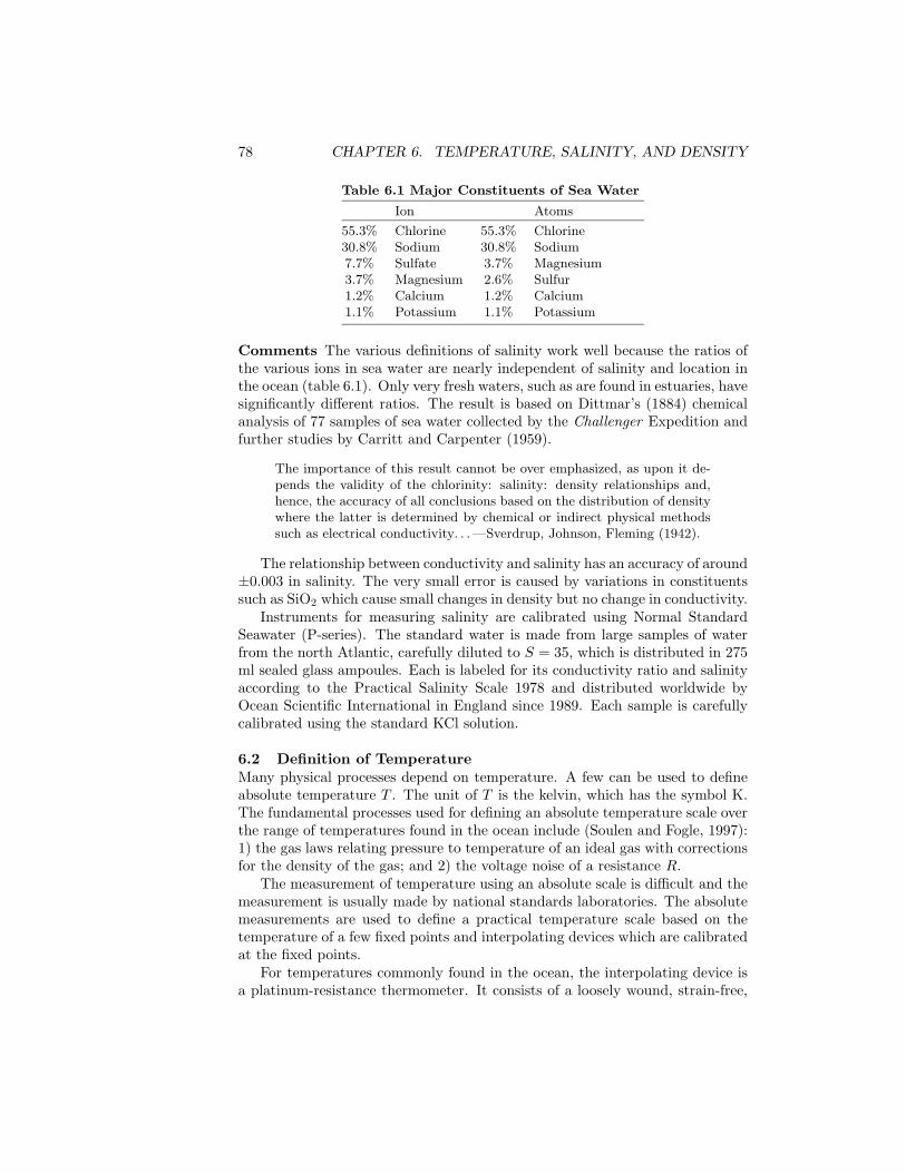
78 CHAPTER 6. TEMPERATURE, SALINITY, AND DENSITY
Table 6.1 Major Constituents of Sea Water
Ion Atoms
55.3% Chlorine 55.3% Chlorine30.8% Sodium 30.8% Sodium7.7% Sulfate 3.7% Magnesium3.7% Magnesium 2.6% Sulfur1.2% Calcium 1.2% Calcium1.1% Potassium 1.1% Potassium
Comments The various definitions of salinity work well because the ratios ofthe various ions in sea water are nearly independent of salinity and location inthe ocean (table 6.1). Only very fresh waters, such as are found in estuaries, havesignificantly different ratios. The result is based on Dittmar’s (1884) chemicalanalysis of 77 samples of sea water collected by the Challenger Expedition andfurther studies by Carritt and Carpenter (1959).
The importance of this result cannot be over emphasized, as upon it de-pends the validity of the chlorinity: salinity: density relationships and,hence, the accuracy of all conclusions based on the distribution of densitywhere the latter is determined by chemical or indirect physical methodssuch as electrical conductivity. . . —Sverdrup, Johnson, Fleming (1942).
The relationship between conductivity and salinity has an accuracy of around±0.003 in salinity. The very small error is caused by variations in constituentssuch as SiO2 which cause small changes in density but no change in conductivity.
Instruments for measuring salinity are calibrated using Normal StandardSeawater (P-series). The standard water is made from large samples of waterfrom the north Atlantic, carefully diluted to S = 35, which is distributed in 275ml sealed glass ampoules. Each is labeled for its conductivity ratio and salinityaccording to the Practical Salinity Scale 1978 and distributed worldwide byOcean Scientific International in England since 1989. Each sample is carefullycalibrated using the standard KCl solution.
6.2 Definition of TemperatureMany physical processes depend on temperature. A few can be used to defineabsolute temperature T . The unit of T is the kelvin, which has the symbol K.The fundamental processes used for defining an absolute temperature scale overthe range of temperatures found in the ocean include (Soulen and Fogle, 1997):1) the gas laws relating pressure to temperature of an ideal gas with correctionsfor the density of the gas; and 2) the voltage noise of a resistance R.
The measurement of temperature using an absolute scale is difficult and themeasurement is usually made by national standards laboratories. The absolutemeasurements are used to define a practical temperature scale based on thetemperature of a few fixed points and interpolating devices which are calibratedat the fixed points.
For temperatures commonly found in the ocean, the interpolating device isa platinum-resistance thermometer. It consists of a loosely wound, strain-free,

6.3. GEOGRAPHICAL DISTRIBUTION 79
pure platinum wire whose resistance is a function of temperature. It is calibratedat fixed points between the triple point of equilibrium hydrogen at 13.8033 Kand the freezing point of silver at 961.78 K, including the triple point of waterat 0.060C, the melting point of Gallium at 29.7646C, and the freezing pointof Indium at 156.5985C (Preston-Thomas, 1990). The triple point of water isthe temperature at which ice, water, and water vapor are in equilibrium. Thetemperature scale in kelvin T is related to the temperature scale in degreesCelsius t/C by:
t [C] = T [K] − 273.15 (6.5)
The practical temperature scale was revised in 1887, 1927, 1948, 1968, and1990 as more accurate determinations of absolute temperature became accepted.The most recent scale is the International Temperature Scale of 1990 (its-90).It differs slightly from the International Practical Temperature Scale of 1968ipts-68. At 0C they are the same, and above 0C its-90 is slightly cooler.t90 − t68 = −0.002 at 10C, −0.005 at 20C, −0.007 at 30C and −0.010 at40C.
Notice that while oceanographers use thermometers calibrated with an ac-curacy of a millidegree, which is 0.001C, the temperature scale itself has un-certainties of a few millidegrees.
6.3 Geographical Distribution of Surface Temperature and SalinityThe distribution of temperature at the sea surface tends to be zonal, that is, it isindependent of longitude (figure 6.2). Warmest water is near the equator, coldestwater is near the poles. The deviations from zonal are small. Equatorward of40, cooler waters tend to be on the eastern side of the basin. North of thislatitude, cooler waters tend to be on the western side.
The anomalies of sea-surface temperature, the deviation from a long termaverage, are small, less than 1.5C (Harrison and Larkin, 1998) except in theequatorial Pacific where the deviations can be 3C (figure 6.3: top).
The annual range of surface temperature is highest at mid-latitudes, espe-cially on the western side of the ocean (figure 6.3: bottom). In the west, cold airblows off the continents in winter and cools the ocean. The cooling dominatesthe heat budget. In the tropics the temperature range is mostly less than 2C.
The distribution of sea-surface salinity also tends to be zonal. The saltiestwaters are at mid-latitudes where evaporation is high. Less salty waters are nearthe equator where rain freshens the surface water, and at high latitudes wheremelted sea ice freshens the surface waters (figure 6.4). The zonal (east-west)average of salinity shows a close correlation between salinity and evaporationminus precipitation plus river input (figure 6.5).
Because many large rivers drain into the Atlantic and the Arctic Sea, whyis the Atlantic saltier than the Pacific? Broecker (1997) showed that 0.32 Sv ofthe water evaporated from the Atlantic does not fall as rain on land. Instead,it is carried by winds into the Pacific (figure 6.6). Broecker points out that thequantity is small, equivalent to a little more than the flow in the Amazon River,

80 CHAPTER 6. TEMPERATURE, SALINITY, AND DENSITY
Average Sea-Surface Temperature for January
0 0
55
1010
1515
2020
25
25
2525
28
28
28
25 2520
2015 15
1010
5 5
5 5
00
00
20o 60o 100o 140o 180o -140o -100o -60o -20o 20o-90o
-60o
-30o
0o
30o
60o
90o
0o
Average Sea-Surface Temperature for July
00
55
10 101515
20
20
20
25252525
2525
25
20
20
15
15
10
10
55
50
00
28
28
2828
20o 60o 100o 140o 180o -140o -100o -60o -20o 20o-90o
-60o
-30o
0o
30o
60o
90o
0o
Figure 6.2 Mean sea-surface temperature calculated from the optimal interpolation technique(Reynolds and Smith, 1995) using ship reports and avhrr measurements of temperature.Contour interval is 1C with heavy contours every 5C. Shaded areas exceed 29C.
but “were this flux not compensated by an exchange of more salty Atlanticwaters for less salty Pacific waters, the salinity of the entire Atlantic would riseabout 1 gram per liter per millennium.”
Mean Temperature and Salinity of the Ocean The mean temperature of theocean’s waters is: t = 3.5C. The mean salinity is S = 34.7. The distributionabout the mean is small: 50% of the water is in the range:
1.3C < t < 3.8C34.6 < S < 34.8

6.4. THE OCEANIC MIXED LAYER AND THERMOCLINE 81
1 1222
3 33 3
4
4
44
4 46
5
33
33
33 2
44
44
5
544 4 4
11
112 2 2 2 33
339
10
8
6
67
3
24
44
3 3
5
15
12
4
5
5
55
555 6
6
6
6
67
11
12
14
9864
78
91011121314
14151617
22
2 2
5
5
5 5
5
62 1
7 896
32
1
22
56
2
7
7
8
8
8
9
9
10111213141516
17
1819207
10
11
5
6
16
17
Annual Range of Sea-Surface Temperature
20o 60o 100o 140o 180o -140o -100o -60o -20o 20o-90o
-60o
-30o
0o
30o
60o
90o
0o
0
0
0
0 1
1
0
0
0
0
0
0
0
00
1
00
0
1
0
0
1
10
1
1
1
000
1
00
0
11
Optimal Interpolation Monthly SST Anomalies for Jan. 1996
20o 60o 100o 140o 180o -140o -100o -60o -20o 20o-90o
-60o
-30o
0o
30o
60o
90o
0o
Figure 6.3 Top: Sea-surface temperature anomaly for January 1996 relative to meantemperature shown in figure 6.2 using data published by Reynolds and Smith (1995) in theClimate Diagnostics Bulletin for February 1995. Contour interval is 1C. Shaded areasare positive. Bottom:Annual range of sea-surface temperature in C calculated from theReynolds and Smith (1995) mean sea-surface temperature data set. Contour interval is 1Cwith heavy contours at 4C and 8C. Shaded areas exceed 8C.
6.4 The Oceanic Mixed Layer and Thermocline
Wind blowing on the ocean stirs the upper layers leading to a thin mixed layer atthe sea surface having constant temperature and salinity from the surface downto a depth where the values differ from those at the surface. The magnitude ofthe difference is arbitrary, but typically the temperature at the bottom of thelayer must be no more than 0.02–0.1 colder than at the surface. Note that theboth temperature and salinity must be constant in the mixed layer. We will see

82 CHAPTER 6. TEMPERATURE, SALINITY, AND DENSITY
Annual Mean Sea Surface Salinity
34
34
35 35
35
35
35
35
3637
34
34
34
34
34
33
33
33
33
33
32
32
32 32
32
36
3735
35 34
34
31
30
30
30 30
3031
37
3332
36
34
34
34 36
34 35
34 33
3231
35
29
39
20o 60o 100o 140o 180o -140o -100o -60o -20o 20o-90o
-60o
-30o
0o
30o
60o
90o
0o
Figure 6.4 Mean sea-surface salinity. Contour interval is 0.25 psu.Shaded areas exceed 36 psu. From Levitus (1982).
later that mean velocity is not constant. The mixed layer is roughly 10–200 mthick over most of the tropical and mid-latitude belts.
The depth and temperature of the mixed layer varies from day to day andfrom season to season in response to two processes:
1. Heat fluxes through the surface heat and cool the surface waters. Changesin temperature change the density contrast between the mixed layer anddeeper waters. The greater the contrast, the more work is needed to mixthe layer downward and visa versa.
2. Turbulence in the mixed layer mixes heat downward. The turbulence
evaporation - precipitation
salinity
Eva
pora
tion
- pr
ecip
itatio
n (m
/yr)
0.5
1.0
-1.5
-1.0
-0.5
0.0
-90o -60o -30o 0o 30o 60o 90o
30
32
34
36S
alin
ity (
psu
)
Figure 6.5 Zonal average of sea-surface salinity calculated for all oceans from Levitus (1982)and the difference between evaporation and precipitation (E−P ) calculated from data shownin figure 5.14.

6.4. THE OCEANIC MIXED LAYER AND THERMOCLINE 83
0.23 +0.03
-0.32 Sv
0.36
0.07
0.20
0.19-0.17
-0.18 0.25
Desert
Desert
0o 30o 60o 90o 120o 150o 180o-30o-60o-90o-120o-150o180o
75o
60o
45o
30o
15o
0o
-15o
-30o
-45o
-60o
Figure 6.6 Water transported by the atmosphere into and out of the Atlantic. Basinsdraining into the Atlantic are black, deserts are white, and other drainage basins are shaded.Arrows give direction of water transport by the atmosphere, and values are in Sverdrups.Bold numbers give the net transport for the Atlantic. Overall, the Atlantic loses 0.32 Sv, anamount approximately equal to the flow in the Amazon River. After Broecker (1997).
Sept 90
Aug 90
Nov 89
Jan 90
April 90
30o28o26o24o22o20o18o
0
50
100
150
200
Temperature (Celsius)
Pre
ssur
e (d
ecib
ars)
Figure 6.7 Growth and decay of the mixed layer and seasonal thermocline from November1989 to September 1990 at the Bermuda Atlantic Time-series Station (bats) at 31.8N64.1W. Data were collected by the Bermuda Biological Station for Research, Inc. Notethat pressure in decibars is nearly the same as depth in meters (see §6.8 for a definition ofdecibars).

84 CHAPTER 6. TEMPERATURE, SALINITY, AND DENSITY
depends on the wind speed and on the intensity of breaking waves. Tur-bulence mixes water in the layer, and it mixes the water in the layer withwater in the thermocline.
The mid-latitude mixed layer is thinnest in late summer when winds areweak, and sunlight warms the surface layer (figure 6.7). At times, the heatingis so strong, and the winds so weak, that the layer is only a few meters thick. Infall, the first storms of the season mix the heat down into the ocean thickeningthe mixed layer, but little heat is lost. In winter, heat is lost, and the mixedlayer continues to thicken, becoming thickest in late winter. In spring, windsweaken, sunlight increases, and a new mixed layer forms.
Below the mixed layer, water temperature decreases rapidly with depth ex-cept at high latitudes. The range of depths where the rate of change, thegradient of temperature, is large is called the thermocline. Because density isclosely related to temperature, the thermocline also tends to be the layer wheredensity gradient is greatest, the pycnocline.
The top of the thermocline varies slightly with the seasons as seen in theregion between 20 and 200 decibars in figure 6.7. This is the seasonal thermo-cline. The permanent thermocline extends from below the seasonal thermoclineto depths of 1500–2000 meters (figure 6.8). At high latitudes, such as at the aac
AAC
Winter
Summer
WarmPool
BATS
AAC
WarmPool
BATS
SalinityTemperature (Celsius)
34 35 36 370o 10o 20o 30o
0
500
1000
1500
Pre
ssur
e (d
ecib
ars)
Figure 6.8 Typical temperature and salinity profiles in the open ocean. AAC: At 62.0 S,170.0 E in the Antarctic Circumpolar Current on 16 January 1969 as measured by the R/VHakuho Maru. Warm Pool: At 9.5 N 176.3 E in the tropical west Pacific warm pool on 12March 1989 as measured by Bryden and Hall on the R/V Moana Wave. bats: At 31.8 N64.1 W near Bermuda on 17 April and 10 September 1990 as measured by the BermudaBiological Station for Research, Inc. Data are included with Java OceanAtlas.

6.5. DENSITY 85
station in the figure, there may be a cooler, fresher layer above the permanentthermocline.
The mixed layer tends to be saltier than the thermocline between 10 and40 latitude, where evaporation exceeds precipitation. At high latitudes themixed layer is fresher because rain and melting ice reduce salinity. In sometropical regions, such as the warm pool in the western tropical Pacific, rain alsoproduces a thin fresher mixed layer.
6.5 Density, Potential Temperature, and Neutral DensityDuring winter, cold water formed at the surface sinks to a depth determined byits density relative to the density of the deeper water. Currents then carry thewater to other parts of the ocean. At all times, the water parcel moves to staybelow less dense water and above more dense water. The distribution of currentswithin the ocean depends on the distribution of pressure, which depends on thevariations of density inside the ocean as outlined in §10.4. So, if we want tofollow water movement within the ocean, we need to know the distribution ofdensity within the ocean.
Density and sigma-t The calculation of water movement requires measure-ments of density with an accuracy of a few parts per million. This is not easy.
Absolute Density of water can only be measured in spacial laboratories, andonly with difficulty. The best accuracy is 1 : 2.5 × 105 = 4 parts per million.
To avoid the difficulty of working with absolute density, oceanographers usedensity relative to density of pure water. Density ρ(S, t, p) is now defined usingStandard Mean Ocean Water of known isotopic composition, assuming satura-tion of dissolved atmospheric gasses. Here S, t, p refers to salinity, temperature,and pressure.
In practice, density is not measured, it is calculated from in situ measure-ments of pressure, temperature, and conductivity using the equation of statefor sea water. This can be done with an accuracy of two parts per million.
Density of water at the sea surface is typically 1027 kg/m3. For simplifica-tion, physical oceanographers often quote only the last 2 digits of the density,a quantity they call density anomaly or Sigma (s,t,p):
σ(S, t, p) = ρ(S, t, p) − 1000 kg/m3 (6.6)
σ(S, t, p) is typically 27.00 kg/m3. The Working Group on Symbols in Oceanog-raphy recommends that σ be replaced by γ because σ was originally definedrelative to pure water and it was dimensionless. Here, however, we will followcommon practice and use σ.
If we are studying surface layers of the ocean, we can ignore compressibility,and we use a new quantity sigma-t (written σt):
σt = σ(S, t, 0) (6.7)
This is the density anomaly of a water sample when the total pressure on ithas been reduced to atmospheric pressure (i.e. zero water pressure), but thetemperature and salinity are in situ values.

86 CHAPTER 6. TEMPERATURE, SALINITY, AND DENSITY
σt
t
θ
σθ
Density
2827.5 27.6 27.7 27.927.8
-8000
-7000
-6000
-5000
-3000
-2000
-10005o0o
Temperature (Celsius)
1o 2o 3o 4o
-4000
Dep
th (
m)
Figure 6.9 Profiles of Left in situ t and potential θ temperature and Right sigma-t andsigma-theta in the Kermadec Trench in the Pacific measured by the R/V Eltanin during theScorpio Expedition on 13 July 1967 at 175.825 E and 28.258 S. Data from Warren (1973).
Potential Temperature As a water parcel moves within the ocean below themixed layer, its salt and heat content can change only by mixing with otherwater. Thus we can use measurements of temperature and salinity to trace thepath of the water. This is best done if we remove the effect of compressibility.
As water sinks, pressure increases, the water is compressed, and the com-pression does work on the water. This causes the water to warm. To understandthe warming, consider a cube containing a fixed mass of water. As the cubesinks, its sides move inward as the cube is compressed. Recalling that work isforce times distance, the work is the distance the side moves times the forceexerted on the side by pressure. The heating is small but noticeable comparedwith the small changes of the temperature of the adjacent water (figure 6.9).At a depth of 8km, the increase in temperature is almost 0.9 C.
To remove the influence of compressibility from measurements of temper-ature, oceanographers (and meteorologists who have the same problem in theatmosphere) use the concept of potential temperature. Potential temperatureΘ is defined as the temperature of a parcel of water at the sea surface after ithas been raised adiabatically from some depth in the ocean. Raising the parceladiabatically means that it is raised in an insulated container so it does not ex-

6.5. DENSITY 87
change heat with its surroundings. Of course, the parcel is not actually broughtto the surface. Potential temperature is calculated from the temperature in thewater at depth, the in situ temperature.
Potential Density If we are studying intermediate layers of the ocean, sayat depths near a kilometer, we cannot ignore compressibility. Because changesin pressure primarily influence the temperature of the water, the influence ofpressure can be removed, to a first approximation, by using the potential density.
Potential density ρΘ is the density a parcel of water would have if it wereraised adiabatically to the surface without change in salinity. Written as sigma,
σΘ = σ(s,Θ, 0) (6.8)
σΘ is especially useful because it is a conserved thermodynamic property.Potential density is not useful for comparing density of water at great depths.
If we bring water parcels to the surface and compare their densities, the calcu-lation of potential density ignores the effect of pressure on the coefficients forthermal and salt expansion. As a result, two water samples having the samedensity but different temperature and salinity at a depth of four kilometers canhave noticeably different potential density. In some regions the use of ρ(Θ) canlead to an apparent decrease of density with depth (figure 6.10) although weknow that this is not possible because such a column of water would be unstable.
To compare samples from great depths, it is better to bring both samples toa nearby depth instead of to the surface p = 0. For example, we can bring bothparcels to a pressure of 4,000 decibars, which is near a depth of 4 km:
σ4 = σ(s,Θ, 4000) (6.9)
where σ4 is the density of a parcel of water brought adiabatically to a pressureof 4,000 decibars. More generally, oceanographers sometimes use ρr
σr = σ(s,Θ, p, pr) (6.10)
where where p is pressure, and pr is pressure at some reference level. In (6.8)the level is pr = 0 decibars, and in (6.9) pr = 4000 decibars.
The use of σr leads to problems. If we wish to follow parcels of water deepin the ocean, we might use σ3 in some areas, and σ4 in others. But whathappens when a parcel moves from a depth of 3 km in one area to a depthof 4 km in another? There is a small discontinuity between the density of theparcel expressed as σ3 compared with density expressed as σ4. To avoid thisdifficulty, Jackett and McDougall (1997) proposed a new variable they calledneutral density.
Neutral Surfaces and Density A parcel of water moves locally along a pathof constant density keeping below less dense water and above more dense water.More precisely, it moves along a path of constant potential density σr referencedto the local depth r. Such a path is called a neutral path (Eden and Willebrand,1999). A neutral surface element is the surface tangent to the neutral paths

88 CHAPTER 6. TEMPERATURE, SALINITY, AND DENSITY
7000
6000
5000
4000
3000
2000
1000
0m
-80o
ANTARCTICA
GREENLAND-ICELANDRIDGE
-60o -40o -20o 0o 20o 40o 60o 80o
28.08
28.027.727.927.7
27.8
26.025.0
26.024.026.0
27.0
27.427.6
27.727.8
27.2 27.0
27.88 27.85
27.88 27.88
27.9
27.92
27.8527.9
27.94
46.046.1
45.645.4
45.043.0
41.0
45.2
45.645.6
45.7
45.445.044.0
45.7
45.6 45.645.545.4
45.445.2
46.0
46.4
>46.4
46.4
46.246.1
45.945.8
46.0 45.95
45.945.8
45.9346.0
43.042.0
40.0
7000
6000
5000
4000
3000
2000
1000
0m
-80o
ANTARCTICA
GREENLAND-ICELANDRIDGE
-60o -40o -20o 0o 20o 40o 60o 80o
Pre
ssur
e (d
ecib
ars)
σ4000
σtheta
Figure 6.10 Vertical sections of density in the western Atlantic. Note that the depth scalechanges at 1000 m depth. Upper: σΘ, showing an apparent density inversion below 3,000 m.Lower: σ4 showing continuous increase in density with depth. After Lynn and Reid (1968).
through a point in the water. No work is required to move a parcel on thissurface because there is no buoyancy force acting on the parcel as it moves (ifwe ignore friction).
Now let’s follow the parcel as it moves away from a local region. This can bedone approximately but not exactly. At first we might think that because weknow the tangents to the surface everywhere, we can define a surface that is theenvelope of the tangents. But an exact surface is not mathematically possiblein the real ocean, although we can come very close.
Jackett and McDougall (1997) developed a practical neutral density variableγn and surface that stays within a few tens meters of an ideal surface anywherein the world. They constructed their variables using data in the Levitus (1982)atlas. The neutral density values were then used to label the data in the Levitusatlas. This prelabeled data set is used to calculate γn at new locations where t, Sare measured as a function of depth by interpolation to the four closest pointsin the Levitus atlas. Through this practice, neutral density γn is a function ofsalinity S, in situ temperature t, pressure p, longitude, and latitude.
The neutral surface defined above differs only slightly from an ideal neutralsurface. If a parcel moves around a gyre on the neutral surface and returns toits starting location, its depth at the end will differ by around 10 meters fromthe depth at the start. If potential density surfaces are used, the difference can

6.6. MEASUREMENT OF TEMPERATURE 89
be hundreds of meters, a far larger error.
Equation of state of sea water Density of sea water is rarely measured.Density is calculated from measurements of temperature, conductivity, or salin-ity, and pressure using the equation of state of sea water. The equation of stateis an equation relating density to temperature, salinity, and pressure.
The equation is derived by fitting curves through laboratory measurementsof density as a function of temperature, pressure, and salinity, chlorinity, orconductivity. The International Equation of State (1980) published by the JointPanel on Oceanographic Tables and Standards (1981) is now used. See alsoMillero and Poisson (1981) and Millero et al (1980). The equation has anaccuracy of 10 parts per million, which is 0.01 units of σ(Θ).
I have not actually written out the equation of state because it consists ofthree polynomials with 41 constants (jpots, 1991).
Accuracy of Temperature, Salinity, and Density If we want to distin-guish between different water masses in the ocean, and if the total range oftemperature and salinity is as small as the range in figure 6.1, then we mustmeasure temperature, salinity, and pressure very carefully. We will need anaccuracy of a few parts per million.
Such accuracy can be achieved only if all quantities are carefully defined, ifall measurements are made with great care, if all instruments are carefully cali-brated, and if all work is done according to internationally accepted standards.The standards are laid out in Processing of Oceanographic Station Data (jpots,1991) published by unesco. The book contains internationally accepted defini-tions of primary variables such as temperature and salinity and methods for themeasuring the primary variables. It also describes accepted methods for calcu-lating quantities derived from primary variables, such as potential temperature,density, and stability.
6.6 Measurement of TemperatureTemperature in the ocean has been measured many ways. Thermistors and mer-cury thermometers are commonly used on ships and buoys. These are calibratedin the laboratory before being used, and after use if possible, using mercury orplatinum thermometers with accuracy traceable to national standards laborato-ries. Infrared radiometers on satellites measure the ocean’s surface temperature.
Mercury Thermometer This is the most widely used, non-electronic ther-mometer. It was widely used in buckets dropped over the side of a ship to mea-sure the temperature of surface waters, on Nansen bottles to measure subseatemperatures, and in the laboratory to calibrate other thermometers. Accuracyis about ±0.001C with careful calibration.
One very important mercury thermometer is the reversing thermometer (fig-ure 6.11) carried on Nansen bottles, which are described in the next section. Itis a thermometer that has a constriction in the mercury capillary that causesthe thread of mercury to break at a precisely determined point when the ther-mometer is turned upside down. The thermometer is lowered deep into the

90 CHAPTER 6. TEMPERATURE, SALINITY, AND DENSITY
ocean in the normal position, and it is allowed to come to equilibrium withthe water. Mercury expands into the capillary, and the amount of mercury inthe capillary is proportional to temperature. The thermometer is then flippedupside down, the thread of mercury breaks trapping the mercury in the capil-lary, and the thermometer is brought back. The mercury in the capillary of thereversed thermometer is read on deck along with the temperature of a normalthermometer, which gives the temperature at which the reversed thermometeris read. The two readings give the temperature of the water at the depth wherethe thermometer was reversed.
2
1
0
1
2
3
4
5
6
7
8
9
1 1
10
4 1
12
13
15
0 6
0 5
0 4
0 3
0
0 2
0 1
102
1
0
1
2
3
4
5
6
7
8
9
1 1
10
4 1
12
13
15
0 6
0 5
0 4
0 3
0
0 2
0 1
10
Figure 6.11 Left: Protected and unprotected reversing thermometers is set position, beforereversal. Right: The constricted part of the capillary in set and reversed positions. Aftervon Arx (1962: 259).

6.6. MEASUREMENT OF TEMPERATURE 91
The reversing thermometer is carried inside a glass tube which protectsthe thermometer from the ocean’s pressure because high pressure can squeezeadditional mercury into the capillary. If the thermometer is unprotected, theapparent temperature read on deck is proportional to temperature and pressureat the depth where the thermometer was flipped. A pair of protected andunprotected thermometers gives temperature and pressure of the water at thedepth the thermometer was reversed.
Pairs of reversing thermometers carried on Nansen bottles were the primarysource of subsea measurements of temperature as a function of pressure fromaround 1900 to 1970.
Platinum Resistance Thermometer This is the standard for temperature.It is used by national standards laboratories to interpolate between definedpoints on the practical temperature scale. It is used primarily to calibrate othertemperature sensors.
Thermistor A thermistor is a semiconductor having resistance that variesrapidly and predictably with temperature. It has been widely used on mooredinstruments and on instruments deployed from ships since about 1970. It hashigh resolution and an accuracy of about ±0.001C when carefully calibrated.
Bucket temperatures The temperature of surface waters has been routinelymeasured at sea by putting a mercury thermometer into a bucket which islowered into the water, letting it sit at a depth of about a meter for a fewminutes until the thermometer comes to equilibrium, then bringing it aboardand reading the temperature before water in the bucket has time to changetemperature. The accuracy is around 0.1C. This is a very common source ofdirect surface temperature measurements.
Ship Injection Temperature The temperature of the water drawn into theship to cool the engines has been recorded routinely for decades. These recordedvalues of temperature are called injection temperatures. Errors are due to ship’sstructure warming water before it is recorded. This happens when the tempera-ture recorder is not placed close to the point on the hull where water is broughtin. Accuracy is 0.5–1C.
Advanced Very High Resolution Radiometer The most commonly usedinstrument to measure sea-surface temperature from space is the Advanced VeryHigh Resolution Radiometer avhrr. The instrument has been carried on allpolar-orbiting meteorological satellites operated by noaa since Tiros-N waslaunched in 1978.
The instrument was originally designed to measure cloud temperatures andhence cloud height. The instrument had, however, sufficient accuracy and preci-sion that it was soon used to measure regional and global temperature patternsat the sea surface.
The instrument is a radiometer that converts infrared radiation into electricalsignals. It includes a mirror that scans from side to side across the subsatellitetrack and reflects radiance from the ground into a telescope, a telescope that fo-

92 CHAPTER 6. TEMPERATURE, SALINITY, AND DENSITY
cuses the radiance on detectors, detectors sensitive to different wavelengths thatconvert the radiance at those wavelengths into electrical signals, and electroniccircuitry to digitize and store the radiance values. The instruments observes a2700-km wide swath centered on the subsatellite track. Each observation alongthe scan is from a pixel that is roughly one kilometer in diameter near the centerof the scan and that increases in size with distance from the subsatellite track.
The radiometers measures infrared radiation emitted from the surface infive wavelength bands: three infrared bands: 3.55–3.99 µm, 10.3–11.3 µm, and11.5–12.5 µm; a near-infrared band at 0.725–1.10 µm; and a visible-light bandat 0.55–0.90 µm. All infrared bands include radiation emitted from the sea andfrom water vapor in the air along the path from the satellite to the ground. The3.7 µm band is least sensitive to water vapor and other errors, but it works onlyat night because sunlight has radiance in this band. The two longest wavelengthbands at 10.8 µm and 12.0 µm are used to observe sea-surface temperature andwater vapor along the path in daylight.
Data with 1-km resolution are transmitted directly to ground stations thatview the satellite as it passes the station. This is the Local Area Coveragemode. Data are also averaged to produce observations from 4 × 4 km pixels.These data are stored on tape recorders and later transmitted to noaa receivingstations. This is the Global Area Coverage mode.
The swath width is sufficiently wide that the satellite views the entire earthtwice per day, at approximately 09:00 AM and 9:00 PM local time. Areas athigh latitudes may be observed as often as eight or more times per day.
The most important errors are due to:
1. Unresolved or undetected clouds: Large, thick clouds are obvious in theimages of water temperature Thin clouds such as low stratus and highcirrus produce much small errors that are difficult or almost impossible todetect. Clouds smaller in diameter than 1 km, such as trade-wind cumuli,are also difficult to detect. Special techniques have been developed fordetecting small clouds (figure 6.12).
2. Water vapor, which absorbs part of the energy radiated from the seasurface: Water vapor reduces the apparent temperature of the sea surface.The influence is different in the 10.8 µm and 12.0 µm channels, allowingthe difference in the two signals to be used to reduce the error.
3. Aerosols, which absorb infrared radiation. They radiate at temperaturesfound high in the atmosphere. Stratospheric aerosols generated by vol-canic eruptions can lower the observed temperatures by up to a few de-grees Celsius. Dust particles carried over the Atlantic from Saharan duststorms can also cause errors.
4. Skin temperature errors. The infrared radiation seen by the instrumentcomes from a layer at the sea surface that is only a few micrometers thick.The temperature in this layer is not quite the same as temperature a meterbelow the sea surface. They can differ by several degrees when winds arelight (Emery and Schussel, 1989). This error is greatly reduced when

6.6. MEASUREMENT OF TEMPERATURE 93
4
T11 - T3.7T116
5
4
3
2
1
00
Local Mean Temperature Difference (K)
321
Loca
l M
axim
um D
iffer
ence
10
5
0270 275 280 285 290 295
Loca
l S
tand
ard
Dev
iatio
n
Local Mean Temperature (K)
Figure 6.12 The influence of clouds on infrared observations. Left: The standard deviationof the radiance from small, partly cloudy areas each containing 64 pixels. The feet of thearch-like distribution of points are the sea-surface and cloud-top temperatures. After Coakleyand Bretherton (1982). Right: The maximum difference between local values of T11 − T3.7
and the local mean values of the same quantity. Values inside the dashed box indicatecloud-free pixels. T11 and T3.7 are the apparent temperatures at 11.0 and 3.7 µm (data fromK. Kelly). After Stewart (1985: 137).
avhrr data are used to interpolate between ship measurements of surfacetemperature.
Maps of temperature processed from Local Area Coverage of cloud-free re-gions show variations of temperature with a precision of 0.1C. These mapsare useful for observing local phenomena including patterns produced by localcurrents. Figure 10.16 shows such patterns off the California coast.
Global maps are made by the U.S. Naval Oceanographic Office, which re-ceives the global avhrr data directly from noaa’s National EnvironmentalSatellite, Data and Information Service in near-real time each day. The dataare carefully processed to remove the influence of clouds, water vapor, aerosols,and other sources of error. Data are then used to produce global maps between±70 with an accuracy of ±0.6C (May et al 1998). The maps of sea-surfacetemperature are sent to the U.S. Navy and to noaa’s National Centers for En-vironmental Prediction. In addition, the office produces daily 100-km globaland 14-km regional maps of temperature.
Global Maps of Sea-Surface Temperature Global, monthly maps of sur-face temperature are produced by the National Centers for Environmental Pre-diction using Reynolds’ (1988, 1993, 1994) optimal-interpolation method. Thetechnique blends ship and buoy measurements of sea-surface temperature withavhrr data processed by the Naval Oceanographic Office in 1 areas for amonth. Essentially, avhrr data are interpolated between buoy and ship re-ports using previous information about the temperature field. Overall accuracyranges from approximately ±0.3 C in the tropics to ±0.5 C near westernboundary currents in the northern hemisphere where temperature gradients arelarge. Maps are available from November 1981. Figures 6.2–6.4 were made bynoaa using Reynolds’ technique.

94 CHAPTER 6. TEMPERATURE, SALINITY, AND DENSITY
Maps of mean temperature have also been made from coads data. Thedata are poorly distributed in time and space except for some areas of thenorthern hemisphere. In addition, Reynolds and Smith (1994) found that shiptemperature data had errors twice as large as temperature errors in data frombuoys and avhrr. Thus, space data processed by Reynolds are more accurate,and better distributed than coads.
Anomalies of sea-surface temperature are calculated using mean sea-surfacetemperature from the period 1950–1979 calculated from coads supplementedwith four years of satellite data 1982–1985 (Reynolds and Smith, 1995).
6.7 Measurement of Conductivity or SalinityConductivity is measured by placing platinum electrodes in seawater and mea-suring the current that flows when there is a known voltage between the elec-trodes. The current depends on conductivity, voltage, and volume of sea waterin the path between electrodes. If the electrodes are in a tube of non-conductingglass, the volume of water is accurately known, and the current is independentof other objects near the conductivity cell (figure 6.13). The best measurementsof salinity from conductivity give salinity with an accuracy of ±0.005 psu.
Before conductivity measurements were widely used, salinity was measuredusing chemical titration of the water sample with silver salts. The best mea-surements of salinity from titration give salinity with an accuracy of ±0.02 psu.
Individual salinity measurements are calibrated using standard seawater.Long-term studies of accuracy use data from measurements of deep water massesof known, stable, salinity. For example, Saunders (1986) noted that temperatureis very accurately related to salinity for a large volume of water contained in thedeep basin of the northwest Atlantic under the Mediterranean outflow. He usedthe consistency of measurements of temperature and salinity made at many hy-drographic stations in the area to estimate the accuracy of temperature, salinityand oxygen measurements. He concluded that the most careful measurementsmade since 1970 have an accuracy of 0.005 psu for salinity and 0.005C for tem-perature. The largest source of salinity error was the error in determination ofthe standard water used for calibrating the salinity measurements.
Cell Terminals
SeawaterFlow Out
Current Field between Electrodes
BorosilicateGlass Cell
Platinum Electrodes (3 places)
SeawaterFlow In
Figure 6.13 A conductivity cell. Current flows through the seawater between platinumelectrodes in a cylinder of borosilicate glass 191 mm long with an inside diameter between theelectrodes of 4 mm. The electric field lines (solid lines) are confined to the interior of the cellin this design making the measured conductivity (and instrument calibration) independentof objects near the cell. This is the cell used to measure conductivity and salinity shown infigure 6.15. From Sea-Bird Electronics.

6.8. MEASUREMENT OF PRESSURE 95
Year
0.000
0.005
0.010
0.015
0.020
0.025
1920 1930 1940 1950 1960 1970 1980 1990 2000
Sal
inity
Acc
urac
y (p
su)
Figure 6.14. Standard deviation of salinity measurements at depths below 1500 m in theSouth Atlantic from 1920 to 1993. Each point is the average of data collected for thedecade centered on the point. The value for 1995 is an estimate of the accuracy of recentmeasurements. From table 1 of Gouretski and Jancke (1995).
Gouretski and Jancke (1995) estimated accuracyof salinity measurements asa function of time. Using high quality measurements from 16,000 hydrographicstations in the south Atlantic from 1912 to 1991, they estimated accuracy byplotting salinity as a function of temperature using all data collected below 1500m in twelve regions for each decade from 1920 to 1990. A plot of accuracy asa function of time since 1920 shows consistent improvement in accuracy since1950 (figure 6.14). Recent measurements of salinity are the most accurate.The standard deviation of modern salinity data collected from all areas in theSouth Atlantic from 1970 to 1993 adjusted as described by Gouretski and Jancke(1995) was 0.0033 psu. More recent instruments such as the Sea-Bird ElectronicsModel 911 Plus have an accuracy of better than 0.005 psu without adjustments.A careful comparison of salinity measured at 43 10’N 14 4.5’W by the 911Plus with historic data collected by Saunders (1986) gives an accuracy of 0.002psu (figure 6.15).
6.8 Measurement of PressurePressure is routinely measured by many different types of instruments. The SIunit of pressure is the pascal (Pa), but oceanographers normally report pressurein decibars (dbar), where:
1 dbar = 104 Pa (6.11)
because the pressure in decibars is almost exactly equal to the depth in meters.Thus 1000 dbar is the pressure at a depth of about 1000 m.
Strain Gage This is the simplest and cheapest instrument, and it is widelyused. Accuracy is about ±1%.

96 CHAPTER 6. TEMPERATURE, SALINITY, AND DENSITY
5262 m
5000 m
depth(dbar)
3000400050005262
911 CTD(PSU)
34.9503 34.9125 34.8997 34.8986
Autosal(PSU)
34.9501 34.9134 34.8995 34.8996
911-Autosal(PSU)
+0.0002 -0.0009 +0.0002 -0.0010
No. Bottles,(sample range)
3 (.0012)4 (.0013)4 (.0011)3 (.0004)
Saunders, P. (1986)
S = 34.698 + 0.098 θ PSU Valid: θ < 2.5o C.
4000 m
3000 m
Salinity, PSS-7834.89 34.96
2.0o
2.5o
Pot
entia
l Tem
pera
ture
(C
elsi
us)
2.7o
2.6o
2.1o
2.2o
2.3o
2.4o
Figure 6.15. Results from a test of the Sea-Bird Electronics 911 Plus CTD in the NorthAtlantic Deep Water in 1992. Data were collected at 43.17 N and 14.08 W from the R/VPoseidon. From Sea-Bird Electronics (1992).
Vibratron Much more accurate measurements of pressure can be made bymeasuring the natural frequency of a vibrating tungsten wire stretched in amagnetic field between diaphragms closing the ends of a cylinder. Pressure dis-torts the diaphragm, which changes the tension on the wire and its frequency.The frequency can be measured from the changing voltage induced as the wirevibrates in the magnetic field. Accuracy is about ±0.1%, or better when tem-perature controlled. Precision is 100–1000 times better than accuracy. Theinstrument is used to detect small changes in pressure at great depths. Snod-grass (1964) obtained a precision equivalent to a change in depth of ±0.8 mmat a depth of 3 km.
Quartz crystal Very accurate measurements of pressure can also be made bymeasuring the natural frequency of a quartz crystal cut for minimum temper-ature dependence. The best accuracy is obtained when the temperature of thecrystal is held constant. The accuracy is ±0.015%, and precision is ±0.001% offull-scale values.
Quartz Bourdon Gage has accuracy and stability comparable to quartz crys-tals. It too is used for long-term measurements of pressure in the deep sea.
6.9 Measurement of Temperature and Salinity with DepthTemperature, salinity, and pressure are measured as a function of depth usingvarious instruments or techniques, and density is calculated from the measure-ments.

6.9. TEMPERATURE AND SALINITY WITH DEPTH 97
Before turning
While itturns
Afterturning
Figure 6.16 Left A CTD ready to be lowered over the side of a ship. From Davis (1987). RightNansen water bottles before (I), during (II), and after (III) reversing. Both instruments areshown at close to the same scale. After Defant (1961: 33).
Bathythermograph (BT) was a mechanical device that measured tempera-ture vs depth on a smoked glass slide. The device was widely used to map thethermal structure of the upper ocean, including the depth of the mixed layerbefore being replaced by the expendable bathythermograph in the 1970s.
Expendable Bathythermograph (XBT) is an electronic device that mea-sures temperature vs depth using a thermistor on a free-falling streamlinedweight. The thermistor is connected to an ohm-meter on the ship by a thincopper wire that is spooled out from the sinking weight and from the mov-ing ship. The xbt is now the most widely used instrument for measuring thethermal structure of the upper ocean. Approximately 65,000 are used each year.
The streamlined weight falls through the water at a constant velocity. Sodepth can be calculated from fall time with an accuracy of ±2%. Temperatureaccuracy is ±0.1C. And, vertical resolution is typically 65 cm. Probes reach todepths of 200 m to 1830 m depending on model.
Nansen Bottles (figure 6.16) were deployed from ships stopped at hydro-graphic stations. Hydrographic stations are places where oceanographers mea-sure water properties from the surface to some depth, or to the bottom, using

98 CHAPTER 6. TEMPERATURE, SALINITY, AND DENSITY
instruments lowered from a ship. Usually 20 bottles were attached at intervalsof a few tens to hundreds of meters to a wire lowered over the side of the ship.The distribution with depth was selected so that most bottles are in the upperlayers of the water column where the rate of change of temperature in the ver-tical is greatest. A protected reversing thermometer for measuring temperaturewas attached to each bottle along with an unprotected reversing thermometerfor measuring depth. The bottle contains a tube with valves on each end tocollect sea water at depth. Salinity was determined by laboratory analysis ofwater sample collected at depth.
After bottles had been attached to the wire and all had been lowered totheir selected depths, a lead weight was dropped down the wire. The weighttripped a mechanism on each bottle, and the bottle flipped over, reversing thethermometers, shutting the valves and trapping water in the tube, and releasinganother weight. When all bottles had been tripped, the string of bottles wasrecovered. The deployment and retrieval typically took several hours.
CTD Mechanical instruments on Nansen bottles were replaced beginning in the1960s by an electronic instrument, called a ctd, that measured conductivity,temperature, and depth (figure 6.16). The measurements are recorded in digitalform either within the instrument as it is lowered from a ship or on the ship.Temperature is usually measured by a thermistor. Conductivity is measured byinduction. Pressure is measured by a quartz crystal. Modern instruments haveaccuracy summarized in table 6.2.
Table 6.2 Summary of Measurement Accuracy
Variable Range Best Accuracy
Temperature 42 C ± 0.001 CSalinity 1 psu ± 0.02 psu by titration
± 0.005 psu by conductivityPressure 10,00 dbar ± 0.65 dbarDensity 2 kg/m3 ± 0.005 kg/m3
Equation of State ± 0.005 kg/m3
6.10 Light in the Ocean and Absorption of LightSunlight in the ocean is important for many reasons: It heats sea water, warmingthe surface layers; it provides energy required by phytoplankton; it is used fornavigation by animals near the surface; and reflected subsurface light is usedfor mapping chlorophyll concentration from space.
Light in the ocean travels at a velocity equal to the velocity of light ina vacuum divided by the index of refraction (n), which is typically n = 1.33.Hence the velocity in water is about 2.25×10⁸ m/s. Because light travels slowerin water than in air, some light is reflected at the sea surface. For light shiningstraight down on the sea, the reflectivity is (n − 1)2/(n + 1)2. For seawater,the reflectivity is 0.02 = 2%. Hence most sunlight reaching the sea surface istransmitted into the sea, little is reflected. This means that sunlight incidenton the ocean in the tropics is mostly absorbed below the sea surface.
6.10. LIGHT IN THE OCEAN AND ABSORPTION OF LIGHT 99
200 500 1000 1500 2000 2500
λ nm
10-2
104
103
102
101
100
10-1
10-3
Abs
orbt
ion
coef
ficie
nt (
m-1
)
Lenoble-Saint Guily (1955), path length: 400 cm;Hulburt (1934)(1945), path length: 364 cm;Sullivan (1963), path length: 132 cm;Clarke-James (1939), path length: 97 cm (Ceresin lined tube);James-Birge (1938), path length: 97 cm (Silver lined tube).
Infra-red
VisibleUV
viol
etbl
uegr
een
yello
wor
ange
red
Figure 6.17 Absorption coefficient for pure water as a function of wavelength λ of theradiation. Redrawn from Morel (1974: 18, 19). See Morel (1974) for references.
The rate at which sunlight is attenuated determines the depth which islighted and heated by the sun. Attenuation is due to absorption by pigmentsand scattering by molecules and particles. Attenuation depends on wavelength.Blue light is absorbed least, red light is absorbed most strongly. Attenuationper unit distance is proportional to the radiance or the irradiance of light:
dI
dx= −c I (6.12)
where x is the distance along beam, c is an attenuation coefficient (figure 6.17),and I is irradiance or irradiance.
Radiance is the power per unit area per solid angle. It is useful for describingthe energy in a beam of light coming from a particular direction. Sometimeswe want to know how much light reaches some depth in the ocean regardless ofwhich direction it is going. In this case we use irradiance, which is the powerper unit area of surface.
If the absorption coefficient is constant, the light intensity decreases expo-nentially with distance.
I2 = I1 exp(−cx) (6.13)

100 CHAPTER 6. TEMPERATURE, SALINITY, AND DENSITY
100
80
60
40
20
0300 400 500 600 700 0.5 2 5 10 20 50 100
-0
-40
-80
-120
-1601
Depth (m
)
Wavelength (µm) Percentage
Tra
nsm
ittan
ce (
%/m
)
I
II
III1
3
5
7
9
1
III
II
IB
I
IA
5
9
Figure 6.18 Left: Transmittance of daylight in the ocean in % per meter as a functionof wavelength. I: extremely pure ocean water; II: turbid tropical-subtropical water; III:mid-latitude water; 1-9: coastal waters of increasing turbidity. Incidence angle is 90forthe first three cases, 45for the other cases. Right: Percentage of 465 nm light reachingindicated depths for the same types of water. After Jerlov (1976).
where I1 is the original radiance or irradiance of light, and I2 is the radiance orirradiance of light after absorption.
Clarity of Ocean Water Sea water in the middle of the ocean is very clear—clearer than distilled water. These waters are a very deep, cobalt, blue—almostblack. Thus the strong current which flows northward offshore of Japan carryingvery clear water from the central Pacific into higher latitudes is known as theBlack Current, or Kuroshio in Japanese. The clearest ocean water is calledType I waters by Jerlov (figure 6.18). The water is so clear that 10% of thelight transmitted below the sea surface reaches a depth of 90 m.
In the subtropics and mid-latitudes closer to the coast, sea water containsmore phytoplankton than the very clear central-ocean waters. Chlorophyll pig-ments in phytoplankton absorb light, and the plants themselves scatter light.Together, the processes change the color of the ocean as seen by observer lookingdownward into the sea. Very productive waters, those with high concentrationsof phytoplankton, appear blue-green or green (figure 6.19). On clear days thecolor can be observed from space. This allows ocean-color scanners, such asthose on SeaWiFS, to map the distribution of phytoplankton over large areas.
As the concentration of phytoplankton increases, the depth where sunlightis absorbed in the ocean decreases. The more turbid tropical and mid-latitudewaters are classified as type II and III waters by Jerlov (figure 6.18). Thusthe depth where sunlight warms the water depends on the productivity of thewaters. This complicates the calculation of solar heating of the mixed layer.
Coastal waters are much less clear than waters offshore. These are the type1–9 waters shown in figure 6.18. They contain pigments from land, sometimescalled gelbstoffe, which just means yellow stuff, muddy water from rivers, andmud stirred up by waves in shallow water. Very little light penetrates morethan a few meters into these waters.

6.10. LIGHT IN THE OCEAN AND ABSORPTION OF LIGHT 101
( < 0.1)0.3
1.3
0.6
3.0
4
3
2
1
00.400 0.500 0.600 0.700
Wavelength (µm)
Ref
lect
ance
(%
)
Figure 6.19 Spectral reflectance of sea water observed from an aircraft flying at 305 m overwaters of different colors in the Northwest Atlantic. The numerical values are the averagechlorophyll concentration in the euphotic (sunlit) zone in units of mg/m3. The reflectanceis for vertically polarized light observed at Brewster’s angle of 53. This angle minimizesreflected skylight and emphasizes the light from below the sea surface. After Clarke, Ewing,and Lorenzen (1970).
Measurement of Chlorophyll from Space The color of the ocean, andhence the chlorophyll concentration in the upper layers of the ocean has beenmeasured by the Coastal Zone Color Scanner carried on the Nimbus-7 satellitelaunched in 1978 and by the Sea-viewing Wide Field-of-view Sensor (SeaWiFS)carried on SeaStar, launched in 1997. The latter instrument measures upwellingradiance in eight wavelength bands between 412 nm and 856 nm.
Most of the upwelling radiance seen by the satellite comes from the atmo-sphere. Only about 10% comes from the sea surface. Both air molecules andaerosols scatter light, and very accurate techniques have been developed to re-move the influence of the atmosphere.
The total radiance Lt received by an instrument in space is:
Lt(λi) = t(λi)LW (λi) + Lr(λi) + La(λi) (6.14)
where λi is the wavelength of the radiation in the band measured by the instru-ment, LW is the radiance leaving the sea surface, Lr is radiance scattered bymolecules, called the Rayleigh radiance, La is radiance scattered from aerosols,
102 CHAPTER 6. TEMPERATURE, SALINITY, AND DENSITY
and t is the transmittance of the atmosphere. Lr can be calculated from theory,and La can be calculated from the amount of red light received at the instru-ment because very little red light is reflected from the water. Therefore LW canbe calculated from the radiance measured at the spacecraft.
Chlorophyll concentration in the water column is calculated from the ratioof LW at two frequencies. Using data from the Coastal Zone Color Scanner,Gordon et al. (1983) proposed
C13 =1.1298[LW (443)LW (550)
]−1.71
(6.15a)
C23 =3.3266[LW (520)LW (550)
]−2.40
(6.15b)
where C is the chlorophyll concentration in the surface layers in mg pigment/m3,and LW (443), LW (520), andLW (550) is the radiance at wavelengths of 443, 520,and 550 nm. C13 is used when C13 ≤ 1.5 mg/m3, otherwise C23 is used.
The technique is used to calculate chlorophyll concentration within a factorof 50% over a wide range of concentrations from 0.01 to 10 mg/m3.
6.11 Important Concepts1. Density in the ocean is determined by temperature, salinity, and pressure.
2. Density changes in the ocean are very small, and studies of water massesand currents require density with an accuracy of 10 parts per million.
3. Density is not measured, it is calculated from measurements of tempera-ture, salinity, and pressure using the equation of state of sea water.
4. Accurate calculations of density require accurate definitions of tempera-ture and salinity and an accurate equation of state.
5. Salinity is difficult to define and to measure. To avoid the difficulty,oceanographers use conductivity instead of salinity. They measure conduc-tivity and calculate density from temperature, conductivity, and pressure.
6. A mixed layer of constant temperature and salinity is usually found in thetop 1–100 meters of the ocean. The depth is determined by wind speedand the flux of heat through the sea surface.
7. To compare temperature and density of water masses at different depths inthe ocean, oceanographers use potential temperature and potential densitywhich remove most of the influence of pressure on density.
8. Water parcels below the mixed layer move along neutral surfaces.
9. Surface temperature of the ocean was usually measured at sea using bucketor injection temperatures. Global maps of temperature combine theseobservations with observations of infrared radiance from the sea surfacemeasured by an avhrr in space.

6.11. IMPORTANT CONCEPTS 103
10. Temperature and conductivity are usually measured digitally as a functionof pressure using a ctd. Before 1960–1970 the salinity and temperaturewere measured at roughly 20 depths using Nansen bottles lowered on a linefrom a ship. The bottles carried reversing thermometers which recordedtemperature and depth and they returned a water sample from that depthwhich was used to determine salinity on board the ship.
11. Light is rapidly absorbed in the ocean. 95% of sunlight is absorbed in theupper 100 m of the clearest sea water. Sunlight rarely penetrates deeperthan a few meters in turbid coastal waters.
12. Phytoplankton change the color of sea water, and the change in color canbe observed from space. Water color is used to measure phytoplanktonconcentration from space.

104 CHAPTER 6. TEMPERATURE, SALINITY, AND DENSITY

Chapter 7
Some Mathematics: TheEquations of Motion
In this chapter we consider the response of a fluid to internal and externalforces. This leads to a derivation of some of the basic equations describingocean dynamics. In the next chapter, we will consider the influence of viscosity,and in chapter 12 we will consider the consequences of vorticity.
Fluid mechanics used in oceanography is based on Newtonian mechanicsmodified by our evolving understanding of turbulence. Conservation of mass,momentum, angular momentum, and energy lead to particular equations havingnames that hide their origins (table 7.1).
Table 7.1 Conservation Laws Leading to Basic Equations of Fluid Motion
Conservation of Mass: Leads to Continuity Equation.Conservation of Energy: Conservation of heat leads to Heat Budgets.
Conservation of mechanical energy leads toWave Equation.
Conservation of Momentum: Leads to Momentum (Navier-Stokes) Eq.Conservation of Angular Momentum: Leads to Conservation of Vorticity.
7.1 Dominant Forces for Ocean DynamicsOnly a few forces are important in physical oceanography: gravity, buoyancydue to difference in density of sea water, and wind stress (table 7.2). Rememberthat forces are vectors. They have magnitude and direction.
1. Gravity is the dominant force. The weight of the water in the oceanproduces pressure, and the varying weight of water in different regionsof the ocean produces horizontal pressure gradients. Changes in gravity,due to the motion of sun and moon relative to earth produces tides, tidalcurrents, and tidal mixing in the interior of the ocean.
2. Buoyancy is the upward or downward force acting on a parcel of waterthat is more or less dense than other water at its level. For example, cold
105

106 CHAPTER 7. THE EQUATIONS OF MOTION
air blowing over the sea cools surface waters causing them to be moredense than the water beneath. The difference in density results in a forcethat causes the water to sink.
3. Wind blowing across the sea surface transfers horizontal momentum tothe sea. The wind drags the water in the direction of the wind, and itcreates turbulence that stirs the upper layers of the sea producing theoceanic mixed layer. In addition, wind blowing over ripples on the surfaceleads to an uneven distribution of pressure over the ripples causing themto grow into waves.
4. Pseudo-forces are apparent forces that arise from motion in curvilinearor rotating coordinate systems. Thus, writing the equations for inertialmotion in a rotating coordinate system leads to additional force termscalled pseudo forces. For example, Newton’s first law states that there isno change in motion of a body unless a resultant force acts on it. Yet abody moving at constant velocity seems to change direction when viewedfrom a rotating coordinate system. The change in direction is attributedto a pseudo-force, the Coriolis force.
5. Coriolis Force is the dominant pseudo-force influencing currents movingin a coordinate system fixed to the earth.
Table 7.2 Forces in Geophysical Fluid Dynamics
Dominant ForcesGravity Gives rise to pressure forces and tides.Wind Stress Forces motion at the sea surface.Buoyancy Result from changes in density, leads to convection.
Other ForcesAtmospheric Pressure Results in inverted barometer effect.Seismic Results in tsunamis driven by earthquakes.
Note that the last two forces are much less important than the first three.
7.2 Coordinate SystemCoordinate systems allow us to find locations in theory and practice. Vari-ous systems are used depending on the size of the features to be described ormapped. I will refer to the simplest systems; descriptions of other systems canbe found in geography and geodesy books.
1. Cartesian Coordinate System is the one I will use most commonly in thefollowing chapters to keep the discussion as simple as possible. We can de-scribe most processes in Cartesian coordinates without the mathematicalcomplexity of spherical coordinates. The standard convention in geophys-ical fluid mechanics is x is to the east, y is to the north, and z is up.
2. f-Plane is a Cartesian coordinate system in which the Coriolis force isassumed constant. It is useful for describing flow in regions small comparedwith the radius of the earth and larger than a few tens of kilometers.

7.3. TYPES OF FLOW IN THE OCEAN 107
3. β-plane is a Cartesian coordinate system in which the Coriolis force isassumed to vary linearly with latitude. It is useful for describing flow overareas as large as ocean basins.
4. Spherical coordinates are used to describe flows that extend over largedistances and in numerical calculations of basin and global scale flows.
7.3 Types of Flow in the oceanMany terms are used for describing the oceans circulation. Here are a few ofthe more commonly used terms for describing currents and waves.
1. General Circulation is the permanent, time-averaged circulation.2. Abyssal also called the Deep Circulation is the circulation of mass, in the
meridional plane, in the deep ocean, driven by mixing.3. Wind-Driven Circulation is the circulation in the upper kilometer of the
ocean forced by the wind. The circulation can be caused by local windsor by winds in other regions.
4. Gyres are wind-driven cyclonic or anticyclonic currents with dimensionsnearly that of ocean basins.
5. Boundary Currents are currents flowing parallel to coasts. Two types ofboundary currents are important:
• Western boundary currents on the western edge of the oceans tendto be fast, narrow jets such as the Gulf Stream and Kuroshio.
• Eastern boundary currents are weak, e.g. the California Current.6. Squirts or Jets are long narrow currents, with dimensions of a few hundred
kilometers, that are nearly perpendicular to west coasts.7. Mesoscale Eddies are turbulent or spinning flows on scales of a few hundred
kilometers.In addition to flow due to currents, there are many types of oscillatory flows
due to waves. Normally, when we think of waves in the ocean, we visualizewaves breaking on the beach or the surface waves influencing ships at sea. Butmany other types of waves occur in the ocean.
1. Planetary Waves depend on the rotation of the earth for a restoring force,and they including Rossby, Kelvin, Equatorial, and Yanai waves.
2. Surface Waves sometimes called gravity waves, are the waves that even-tually break on the beach. The restoring force is due to the large densitycontrast between air and water at the sea surface.
3. Internal Waves are subsea wave similar in some respects to surface waves.The restoring force is due to change in density with depth.
4. Tsunamis are surface waves with periods near 15 minutes generated byearthquakes.
5. Tidal Currents are horizontal currents and currents associated with inter-nal waves driven by the tidal potential.
6. Edge Waves are surface waves with periods of a few minutes confined toshallow regions near shore. The amplitude of the waves drops off expo-nentially with distance from shore.

108 CHAPTER 7. THE EQUATIONS OF MOTION
7.4 Conservation of Mass and SaltConservation of mass and salt can be used to obtain very useful informationabout flows in the ocean. For example, suppose we wish to know the net lossof fresh water, evaporation minus precipitation, from the Mediterranean Sea.We could carefully calculate the latent heat flux over the surface, but there areprobably too few ship reports for an accurate application of the bulk formula.Or we could carefully measure the mass of water flowing in and out of thesea through the Strait of Gibraltar, but the difference is small and perhapsimpossible to measure accurately.
We can, however, calculate the net evaporation knowing the salinity of theflow in Si and out So, together with a rough estimate of the volume of water Vi
flowing in, where Vi is a volume flow in units of m3/s (figure 7.1).
PrecipitationIn
EvaporationOut
P E
Mediterranean
Vo
Sill330 m
River FlowInR
Atlantic Ocean
ViSi = 36.3
So = 37.8
1.75 Sv
Figure 7.1 Schematic diagram of flow into and out of a basin.After Pickard and Emery (1990: 65).
The mass flowing in is, by definition, ρi Vi. If the volume of the sea does notchange, conservation of mass requires:
ρi Vi = ρo Vo (7.1)
where, ρi, ρo are the densities of the water flowing in and out. We can usuallyassume, with little error, that ρi = ρo.
If there is precipitation P and evaporation E at the surface of the basin andriver inflow R, conservation of mass becomes:
Vi + R + P = Vo + E (7.2)
Solving for (Vo - Vi):
Vo − Vi = (R + P ) − E (7.3)
which states that the net flow of water into the basin must balance precipitationplus river inflow minus evaporation when averaged over a sufficiently long time.
Because salt is not deposited or removed from the sea, conservation of saltrequires :
ρi Vi Si = ρo Vo So (7.4)
Where ρi, Si are the density and salinity of the incoming water, and ρo, So aredensity and salinity of the outflow. With little error, we can again assume thatρi = ρo.

7.5. THE TOTAL DERIVATIVE (D/DT) 109
An Example of Conservation of Mass and Salt Pickard and Emery (1990)in Descriptive Physical oceanography applied the theory to flow into the Mediter-ranean Sea using values for salinity given in figure 7.1. The incoming volumeof water has been estimated to be 1.75 × 10⁶ m3/s = 1.75 Sv, where Sv =Sverdrup = 106 m3/s is the unit of volume transport used in oceanography.Solving Eq. 7.4 for Vo assuming that ρi = ρo, and using the estimated value ofVi and the measured salinity gives Vo = 1.68 × 10⁶ m3/s. Eq. (7.3) then gives(R + P − E) = −7 × 10⁴ m3/s.
Knowing Vi, we can also calculate a minimum flushing time for replacingwater in the sea by incoming water. The minimum flushing time Tm is thevolume of the sea divided by the volume of incoming water. The Mediterraneanhas a volume of around 4 × 10⁶ km3. Converting 1.75 × 10⁶ m3/s to km3/yrwe obtain −5.5 × 10⁴ km3/yr. Then, Tm = 4 × 10⁶ km3/−5.5 × 104 km3/yr= 70 yr. The actual time depends on mixing within the sea. If the waters arewell mixed, the flushing time is close to the minimum time, if they are not wellmixed, the flushing time is longer.
Our example of flow into and out of the Mediterranean Sea is an exampleof a box model . A box model replaces large systems, such as the MediterraneanSea, with boxes. Fluids or chemicals or organisms can move between boxes, andconservation equations are used to constrain the interactions within systems.
qin
Particle path
qout δt + ∂t
=∂x
∂qδx + qin
y,v
x,u
z,w
∂q
Figure 7.2 Sketch of flow used for deriving the total derivative.
7.5 The Total Derivative (D/Dt)If the number of boxes in a system increases to a very large number as the sizeof each box shrinks, we eventually approach limits used in differential calculus.For example, if we subdivide the flow of water into boxes a few meters on a side,and if we use conservation of mass, momentum, or other properties within eachbox, we can derive the differential equations governing fluid flow.
Consider the simple example of acceleration of flow in a small box of fluid.The resulting equation is called the total derivative. It relates the accelerationof a particle Du/Dt to derivatives of the velocity field at a fixed point in thefluid. We will use the equation to derive the equations for fluid motion fromNewton’s Second Law which requires calculating the acceleration of a particlespassing a fixed point in the fluid.
We begin by considering the flow of a quantity qin into and qout out of thesmall box sketched in figure 7.2. If q can change continuously in time and space,the relationship between qin and qout is:

110 CHAPTER 7. THE EQUATIONS OF MOTION
qout = qin +∂q
∂tδt +
∂q
∂xδx (7.5)
The rate of change of the quantity q within the volume is:
Dq
Dt=
qout − qin
δt=
∂q
∂t+
∂q
∂x
δx
δt(7.6)
But δx/δt is the velocity u, and therefore:
Dq
Dt=
∂q
∂t+ u
∂q
∂x
In three dimensions, the total derivative becomes:
D
Dt=
∂
dt+ u
∂
∂x+ v
∂
∂y+ w
∂
∂z(7.7a)
D
Dt=
∂
dt+ u · ∇( ) (7.7b)
where u is the vector velocity and ∇ is the operator del of vector field theory(See Feynman, Leighton, and Sands 1964: 2–6).
This is an amazing result. The simple transformation of coordinates fromone following a particle to one fixed in space converts a simple linear derivativeinto a non-linear partial derivative. Now let’s use the equation to calculate thechange of momentum of a parcel of fluid.
7.6 Momentum EquationNewton’s Second Law relates the change of the momentum of a fluid mass dueto an applied force. The change is:
D(mv)Dt
= F (7.8)
where F is force, m is mass, and v is velocity. We have emphasized the need touse the total derivative because we are calculating the force on a particle. Wecan assume that the mass is constant, and (7.8) can be written:
DvDt
=Fm
= fm (7.9)
where fm is force per unit mass.Four forces are important: pressure gradients, Coriolis force, gravity, and
friction. Without deriving the form of these forces (the derivations are given inthe next section), we can write (7.9) in the following form.
DvDt
= − 1ρ∇ p − 2Ω × v + g + Fr (7.10)

7.6. MOMENTUM EQUATION 111
Acceleration equals the negative pressure gradient minus the Coriolis force plusgravity plus other forces. Here g is acceleration of gravity, Fr is friction, andthe magnitude Ω of Ω is the Rotation Rate of earth, 2π radians per sidereal dayor
Ω = 7.292 × 10⁻⁵ radians/s (7.11)
Momentum Equation in Cartesian coordinates: Expanding the derivativein (7.10) and writing the components in a Cartesian coordinate system gives theMomentum Equation:
∂u
∂t+ u
∂u
∂x+ v
∂u
∂y+ w
∂u
∂z= − 1
ρ
∂p
∂x+ 2 Ω v sinϕ + Fx (7.12a)
∂v
∂t+ u
∂v
∂x+ v
∂v
∂y+ w
∂v
∂z= − 1
ρ
∂p
∂y− 2 Ω u sinϕ + Fy (7.12b)
∂w
∂t+ u
∂w
∂x+ v
∂w
∂y+ w
∂w
∂z= − 1
ρ
∂p
∂z+ 2 Ω u cos ϕ − g + Fz (7.12c)
where Fi are the components of any frictional force per unit mass, and ϕ islatitude. In addition, we have assumed that w << v, so the 2 Ω w cos ϕ hasbeen dropped from equation in (7.12a).
Equation (7.12) appears under various names. Leonhard Euler (1707–1783)first wrote out the general form for fluid flow with external forces, and theequation is sometimes called the Euler equation or the acceleration equation.Louis Marie Henri Navier (1785–1836) added the frictional terms, and so theequation is sometimes called the Navier-Stokes equation.
The term 2 Ω u cos ϕ in (7.12c) is small compared with g, and it can beignored in ocean dynamics. It cannot be ignored, however, for gravity surveysmade with gravimeters on moving ships.
p + δp
z
δxy
δy
x
δz
p
Figure 7.3 Sketch of flow used for deriving the pressure term in the momentum equation.
Derivation of Pressure Term Consider the forces acting on the sides of asmall cube of fluid (figure 7.3). The net force δFx in the x direction is
δFx = p δy δz − (p + δp) δy δz
δFx = −δp δy δz

112 CHAPTER 7. THE EQUATIONS OF MOTION
But
δp =∂p
∂xδx
and therefore
δFx = −∂p
∂xδx δy δz
δFx = − ∂p
∂xδV
Dividing by the mass of the fluid δm in the box, the acceleration of the fluid inthe x direction is:
ax =δFx
δm= −∂p
∂x
δV
δm
ax = −1ρ
∂p
∂x(7.13)
The pressure forces and the acceleration due to the pressure forces in the y andz directions are derived in the same way.
The Coriolis Term in the Momentum Equation The Coriolis term existsbecause we describe currents in a reference frame fixed on earth. The derivationof the Coriolis terms is not simple. Henry Stommel, the noted oceanographerat the Woods Hole Oceanographic Institution even wrote a book on the subjectwith Dennis Moore (Stommel & Moore, 1989).
Usually, we just state that the force per unit mass, the acceleration of aparcel of fluid in a rotating system, can be written:
afixed =(
DvDt
)fixed
=(
DvDt
)rotating
+ (2Ω × v) + Ω × (Ω × R) (7.14)
where R is the vector distance from the center of earth, Ω is the angular velocityvector of earth, and v is the velocity of the fluid parcel in coordinates fixed toearth. The term 2Ω× v is the Coriolis force, and the term Ω× (Ω × R) is thecentrifugal acceleration. The latter term is included in gravity (figure 7.4).
The Gravity Term in the Momentum Equation The gravitational attrac-tion of two masses M1 and m is:
Fg =G M1 m
R2
where R is the distance between the masses, and G is the gravitational constant.The vector force Fg is along the line connecting the two masses.
The force per unit mass due to gravity is:
Fg
m= gf =
G ME
R2(7.15)

7.7. CONSERVATION OF MASS: THE CONTINUITY EQUATION 113
gf
g
( x R)- x
Figure 7.4 Downward acceleration g of a body at rest on earth’s surface is the sum ofgravitational acceleration between the body and earth’s mass gf and the centrifugalacceleration due to earth’s rotation Ω × (Ω × R). The surface of an ocean at rest must beperpendicular to g, and such a surface is close to an ellipsoid of rotation. earth’s ellipticity isgreatly exaggerated here.
where ME is the mass of earth. Adding the centrifugal acceleration to (7.15)gives gravity g (figure 7.4):
g = gf − Ω × (Ω × R) (7.16)
Note that gravity does not point toward earth’s center of mass. The cen-trifugal acceleration causes a plumb bob to point at a small angle to the linedirected to earth’s center of mass. As a result, earth’s surface including theocean’s surface is not spherical but it is a prolate ellipsoid. A rotating fluidplanet has an equatorial bulge.
u + δu
z
δxy
δy
x
δz
u, ρρ + δρ
Figure 7.5 Sketch of flow used for deriving the continuity equation.
7.7 Conservation of Mass: The Continuity EquationNow lets derive the equation for the conservation of mass in a fluid. We beginby writing down the flow of mass into and out of a small box (figure 7.5).
Mass flow in = ρ u δz δy
Mass flow out =(
ρ +∂ρ
∂xδx
) (u +
∂u
∂xδx
)δz δy
=(
ρ u + ρ∂u
∂xδx + u
∂ρ
∂xδx +
∂ρ
∂x
∂u
∂xδx2
)δy δz
114 CHAPTER 7. THE EQUATIONS OF MOTION
The mass flux into the volume must be (mass flow in) − (mass flow out)
Mass flux =(
ρ∂u
∂x+ u
∂ρ
∂x+
∂ρ
∂x
∂u
∂xδx
)δx δy δz
The third term inside the parentheses becomes much smaller than the first twoterms as δx → 0, and
Mass flux =∂(ρu)∂x
δx δy δz
In three dimensions:
Mass flux =(
∂(ρu)∂x
+∂(ρv)∂y
+∂(ρw)
∂x
)δx δy δz
The mass flux must be balanced by a change of mass inside the volume, whichis:
∂ρ
∂tδx δy δz
and conservation of mass requires:
∂ρ
∂t+
∂(ρu)∂x
+d(ρv)∂y
+∂(ρw)
∂z= 0 (7.17)
This is the continuity equation for compressible flow, first derived by LeonhardEuler (1707–1783).
The equation can be put in an alternate form by expanding the derivativesof products and rearranging terms to obtain:
∂ρ
∂t+ u
∂ρ
∂x+ v
∂ρ
∂y+ w
∂ρ
∂z+ ρ
∂u
∂x+ ρ
∂v
∂y+ ρ
∂w
∂z= 0
The first four terms constitute the total derivative of density Dρ/Dt from (7.7),and we can write (7.17) as:
1ρ
Dρ
Dt+
∂u
∂x+
∂v
∂y+
∂w
∂z= 0 (7.18)
This is the alternate form for the continuity equation for a compressible fluid.
The Boussinesq Approximation Density is nearly constant in the ocean,and Joseph Boussinesq (1842–1929) noted that we can safely assume densityis constant except when it is multiplied by g in calculations of pressure in theocean. The assumption greatly simplifies the equations of motion.
Boussinesq’s assumption requires that:1. Velocities in the ocean must be small compared to the speed of sound c.
This ensures that velocity does not change the density. As velocity ap-proaches the speed of sound, the velocity field can produces large changesof density such as shock waves.

7.8. SOLUTIONS TO THE EQUATIONS OF MOTION 115
2. The phase speed of waves or disturbances must be small compared withc. Sound speed in incompressible flows is infinite, and we must assumethe fluid is compressible when discussing sound in the ocean. Thus theapproximation is not true for sound. All other waves in the ocean havespeeds small compared to sound.
3. The vertical scale of the motion must be small compared with c2/g, whereg is gravity. This ensures that as pressure increases with depth in theocean, the increase in pressure produces only small changes in density.
The approximations are true for oceanic flows, and they ensure that oceanicflows are incompressible. See Kundu (1990: 79 and 112), Gill (1982: 85), Batch-elor (1967: 167), or other texts on fluid dynamics for a more complete descriptionof the approximation.
Compressibility The Boussinesq approximationBoussinesq Approximation isequivalent to assuming sea water is incompressible. Now let’s see how the as-sumption simplifies the continuity equation. We define the coefficient of com-pressibility
β ≡ − 1V
∂V
∂p= − 1
V
dV
dt
/dp
dt
where V is volume, and p is pressure. For incompressible flows, β = 0, and:
1V
dV
dt= 0
because dp/dt = 0. Remembering that density is mass m per unit volume V ,and that mass is constant:
1V
dV
dt= −V
d
dt
(1V
)= −V
m
d
dt
(m
V
)= − 1
ρ
dρ
dt= − 1
ρ
Dρ
Dt= 0
If the flow is incompressible, (7.18) becomes:
∂u
∂x+
∂v
∂y+
∂w
∂z= 0 (7.19)
This is the Continuity Equation for Incompressible Flows.
7.8 Solutions to the Equations of MotionEquations (7.12) and (7.19) are four equations, the three components of themomentum equation plus the continuity equation, with four unknowns: u, v,w, p. In principle, we ought to be able to solve the equations with appropriateboundary conditions.
Note, however, that these are non-linear partial differential equations. Con-servation of momentum, when applied to a fluid, converted a simple, first-order,ordinary, differential equation for velocity (Newton’s Second Law), which is usu-ally easy to solve, into a non-linear partial differential equation, which is almostimpossible to solve.

116 CHAPTER 7. THE EQUATIONS OF MOTION
Boundary Conditions: In fluid mechanics, we generally assume:
1. No velocity normal to a boundary, which means there is no flow throughthe boundary; and
2. No flow parallel to a solid boundary, which means no slip at the solidboundary.
Solutions We expect that four equations in four unknowns plus boundary con-ditions give a system of equations that can be solved in principle. In practice,solutions are difficult to find even for the simplest flows. First, as far as I know,there are no exact solutions for the equations with friction. There are very fewexact solutions for the equations without friction. Those who are interested inocean waves might note that one such exact solution is Gerstner’s solution forwater waves (Lamb, 1945: 251). Because the equations are almost impossibleto solve, we will look for ways to greatly simplify the equations. Later, we willfind that even numerical calculations are difficult.
Analytical solutions can be obtained for much simplified forms of the equa-tions of motion. Such solutions are used to study processes in the ocean, in-cluding waves. Solutions for oceanic flows with realistic coasts and bathymetricfeatures must be obtained from numerical solutions. In the next few chapterswe seek solutions to simplified forms of the equations. In Chapter 15 we willconsider numerical solutions.
7.9 Important Concepts1. Gravity, buoyancy, and wind are the dominant forces acting on the ocean.
2. Earth’s rotation produces a pseudo force, the Coriolis force.
3. Conservation laws applied to flow in the ocean lead to equations of motion.Conservation of salt, volume and other quantities can lead to deep insightsinto oceanic flow.
4. The transformation from equations of motion applied to fluid parcels toequations applied at a fixed point in space greatly complicates the equa-tions of motion. The linear, first-order, ordinary differential equationsdescribing Newtonian dynamics of a mass accelerated by a force becomenonlinear, partial differential equations of fluid mechanics.
5. Flow in the ocean can be assumed to be incompressible except when de-scribing sound. Density can be assumed to be constant except when den-sity is multiplied by gravity g. The assumption is called the Boussinesqapproximation.
6. Conservation of mass leads to the continuity equation, which has an espe-cially simple form for an incompressible fluid.

Chapter 8
Equations of Motion WithViscosity
Throughout most of the interior of the ocean and atmosphere friction is rel-atively small, and we can safely assume that the flow is frictionless. At theboundaries, friction, in the form of viscosity, becomes important. This thin,viscous layer is called a boundary layer . Within the layer, the velocity slowsfrom values typical of the interior to zero at a solid boundary. If the boundaryis not solid, then the boundary layer is a thin layer of rapidly changing velocitywhereby velocity on one side of the boundary changes to match the velocity onthe other side of the boundary. For example, there is a boundary layer at thebottom of the atmosphere, the planetary boundary layer we described in Chap-ter 3. In the planetary boundary layer, velocity goes from many meters persecond in the free atmosphere to tens of centimeters per second at the sea sur-face. Below the sea surface, another boundary layer, the Ekman layer describedin Chapter 9, matches the flow at the sea surface to the deeper flow.
In this chapter we consider the role of friction in fluid flows, and the stabilityof the flows to small changes in velocity or density.
8.1 The Influence of ViscosityIn the last chapter we wrote the x–component of the momentum equation for afluid in the form (7:12a):
∂u
∂t+ u
∂u
∂x+ v
∂u
∂y+ w
∂u
∂z= − 1
ρ
∂p
∂x+ 2 Ω v sinϑ + Fx (8.1)
where Fx was a frictional force per unit mass. Now we can consider the form ofthis term if it is due to viscosity.
Molecules in a fluid close to a solid boundary sometime strike the boundaryand transfer momentum to it (figure 8.1). Molecules further from the boundarycollide with molecules that have struck the boundary, further transferring thechange in momentum into the interior of the fluid. This transfer of momentum
117

118 CHAPTER 8. EQUATIONS OF MOTION WITH VISCOSITY
z
x
Molecules carry horizontalmomentum perpendicular towall through perpendicular velocity and collisions with other molecules
Velocity
Wall
Figure 8.1 Molecules colliding with the wall and with each other transfermomentum from the fluid to the wall, slowing the fluid velocity.
is molecular viscosity . Molecules, however, travel only micrometers betweencollisions, and the process is very inefficient for transferring momentum even afew centimeters. Molecular viscosity is important only within a few millimetersof a boundary.
Molecular viscosity ρν is the ratio of the stress T tangential to the boundaryof a fluid and the velocity shear at the boundary. So the stress has the form:
Txz = ρν∂u
∂z(8.2)
for flow in the (x, z) plane within a few millimetres of the surface, where ν isthe kinematic molecular viscosity. Typically ν = 10−6 m2/s for water at 20C.
Generalizing (8.2) to three dimensions leads to a stress tensor giving thenine components of stress at a point in the fluid, including pressure, which isa normal stress, and shear stresses. A derivation of the stress tensor is beyondthe scope of this book, but you can find the details in Lamb (1945: §328) orKundu (1990: p. 93). For an incompressible fluid, the frictional force per unitmass in (8.1) takes the from:
Fx =∂
∂x
[ν
∂u
∂x
]+
∂
∂y
[ν
∂u
∂y
]+
∂
∂z
[ν
∂u
∂z
]=
1ρ
[∂Txx
∂x+
∂Txy
∂y+
∂Txz
∂z
](8.3)
8.2 TurbulenceIf molecular viscosity is important only over distances of a few millimeters, and ifit is not important for most oceanic flows, unless of course you are a zooplanktertrying to swim in the ocean, how then is the influence of a boundary transferredinto the interior of the flow? The answer is: through turbulence.
Turbulence arises from the non-linear terms in the momentum equation(u ∂u/∂x, etc.). The importance of these terms is given by a non-dimensionalnumber, the Reynolds Number Re, which is the ratio of the non-linear terms tothe viscous terms:
Re =Non-linear TermsViscous Terms
=
(u
∂u
∂x
)(
ν∂2u
∂x2
) ≈U
U
L
νU
L2
=UL
ν(8.4)

8.2. TURBULENCE 119
WaterValve
Glass Tube
Dye
Figure 8.2 Reynolds apparatus for investigating the transition to turbulence in pipe flow,with photographs of near-laminar flow (left) and turbulent flow (right) in a clear pipe muchlike the one used by Reynolds. After Binder (1949: 88-89).
where, U is a typical velocity of the flow and L is a typical length describingthe flow. You are free to pick whatever U, L might be typical of the flow. Forexample L can be either a typical cross-stream distance, or an along-stream dis-tance. Typical values in the open ocean are U = 0.1 m/s and L = 1 megameter,so Re = 1011. Because non-linear terms are important if Re > 10 – 1000, theyare certainly important in the ocean. The ocean is turbulent.
The Reynolds number is named after Osborne Reynolds (1842–1912) whoconducted experiments in the late 19th century to understand turbulence. Inone famous experiment (Reynolds 1883), he injected dye into water flowing atvarious speeds through a tube (figure 8.2). If the speed was small, the flowwas smooth. This is called laminar flow. At higher speeds, the flow becameirregular and turbulent. The transition occurred at Re = V D/ν ≈ 2000, whereV is the average speed in the pipe, and D is the diameter of the pipe.
As Reynolds number increases above some critical value, the flow becomesmore and more turbulent. Note that flow pattern is a function of Reynold’snumber. All flows with the same geometry and the same Reynolds number havethe same flow pattern. Thus flow around all circular cylinders, whether 1 mmor 1 m in diameter, look the same as the flow at the top of figure 8.3 if theReynolds number is 20. Furthermore, the boundary layer is confined to a verythin layer close to the cylinder, in a layer too thin to show in the figure.
Turbulent Stresses: The Reynolds Stress Prandtl, Karmen and otherswho studied fluid mechanics in the early 20th century, hypothesized that parcelsof fluid in a turbulent flow played the same role in transferring momentumwithin the flow that molecules played in laminar flow. The work led to the ideaof turbulent stresses.
To see how these stresses might arise, consider the momentum equation for

120 CHAPTER 8. EQUATIONS OF MOTION WITH VISCOSITY
S
A B<1 20
S
SS
80,000 1,000,000
E F
Total Head
-2 -1 0
C174
A'
A0.5
0
1 Width
Y
D
A'
5,000 14,480
1
00.5 1
DX/D
Width
D
0
Figure 8.3 Flow past a circular cylinder as a function of Reynolds number between one anda million. From Richardson (1961). The appropriate flows are: A—a toothpick moving at 1mm/s; B—finger moving at 2 cm/s; F—hand out a car window at 60 mph. All flow at thesame Reynolds number has the same streamlines. Flow past a 10 cm diameter cylinder at 1cm/s looks the same as 10 cm/s flow past a cylinder 1 cm in diameter because in both casesRe = 1000.
a flow with mean and a turbulent components of flow:
u = U + u′ ; v = V + v′ ; w = W + w′ ; p = P + p′ (8.5)
where the mean value U is calculated from a time or space average:
U = 〈u〉 =1T
∫ T
0
u(t) dt or U = 〈u〉 =1X
∫ X
0
u(x) dx (8.6)
The non-linear terms in the momentum equation can be written:⟨(U + u′)
∂(U + u′)∂x
⟩=
⟨U
∂U
∂x
⟩+
⟨U
∂u′
∂x
⟩+
⟨u′ ∂U
∂x
⟩+
⟨u′ ∂u′
∂x
⟩⟨
(U + u′)∂(U + u′)
∂x
⟩=
⟨U
∂U
∂x
⟩+
⟨u′ ∂u′
∂x
⟩(8.7)

8.3. CALCULATION OF REYNOLDS STRESS: 121
The second equation follows from the first since 〈U ∂u′/∂x〉 = 0 and 〈u′ ∂U/∂x〉= 0, which follow from the definition of U : 〈U∂u′/∂x〉 = U∂〈u′〉/∂x = 0.
Using (8.7), the continuity equation splits into two equations:
∂U
∂x+
∂V
∂x+
∂W
∂x= 0 (8.8a)
∂u′
∂x+
∂v′
∂x+
∂w′
∂x= 0 (8.8b)
The x-component of the momentum equation becomes:DU
Dt= −1
ρ
∂P
∂x+ 2ΩV sin ϕ
+∂
∂x
[ν
∂U
∂x− 〈u′u′〉
]+
∂
∂y
[ν
∂U
∂y− 〈u′v′〉
]+
∂
∂z
[ν
∂U
∂z− 〈u′w′〉
] (8.9)
Thus the additional force per unit mass due to the turbulence is:
Fx = − ∂
∂x〈u′u′〉 − ∂
∂y〈u′v′〉 − ∂
∂z〈u′w′〉 (8.10)
The terms ρ〈u′u′〉, ρ〈u′v′〉, and ρ〈u′w′〉 transfer eastward momentum (ρu′)in the x, y, and z directions. For example, the term ρ〈u′w′〉 gives the down-ward transport of eastward momentum across a horizontal plane. Because theytransfer momentum, and because they were first derived by Osborne Reynolds,they are called Reynolds Stresses.
8.3 Calculation of Reynolds Stress:The Reynolds stresses such as ∂〈u′w′〉/∂z are called virtual stresses (cf. Gold-stein, 1965: §69 & §81) because we assume that they play the same role as theviscous terms in the equation of motion. To proceed further, we need values orfunctional form for the Reynolds stress. Several approaches are used.
From Experiments We can calculate Reynolds stresses from direct measure-ments of (u′, v′, w′) made in the laboratory or ocean. This is accurate, but hardto generalize to other flows. So we seek more general approaches.
By Analogy with Molecular Viscosity Let’s return to the simple exampleshown in figure 8.1, which shows a boundary layer above a flat plate in the x,y plane. Now let’s assume that the flow above the plate is turbulent. Thisis a very common type of boundary layer flow, and it a type of flow that wewill describe various times in later chapters. It can be wind flow above the seasurface or flow at the bottom boundary layer in the ocean or flow in the mixedlayer at the sea surface.
For flow above a boundary, we assume that flow is constant in the x, ydirection, that the statistical properties of the flow vary only in the z direction,and that the mean flow is steady. Therefore ∂/∂t = ∂/∂x = ∂/∂y = 0, and(8.9) can be written:
2ΩV sinϕ +∂
∂z
[ν
∂U
∂z− 〈u′w′〉
]= 0 (8.11)

122 CHAPTER 8. EQUATIONS OF MOTION WITH VISCOSITY
We now assume, in analogy with (8.2)
−ρ〈u′w′〉 = Txz = ρAz∂U
∂z(8.12)
where Az is an eddy viscosity or eddy diffusivity which replaces the molecularviscosity ν in (8.2). With this assumption,
∂Txz
∂z=
∂
∂z
(Az
∂U
∂z
)≈ Az
∂2U
∂z2(8.13)
where we have assumed that Az is either constant or that it varies more slowlyin the z direction than ∂U/∂z. Later, we will assume that Az ≈ z.
Because eddies can mix heat, salt, or other properties as well as momentum,I will use the term eddy diffusivity. It is more general than eddy viscosity, whichis the mixing of momentum.
The x and y momentum equations for a homogeneous, steady-state, turbu-lent boundary layer above or below a horizontal surface are:
ρfV +∂Txz
∂z= 0 (8.14a)
ρfU − ∂Tyz
∂z= 0 (8.14b)
where f = 2ω sinϕ is the Coriolis parameter, and we have dropped the molecu-lar viscosity term because it is much smaller than the turbulent eddy viscosity.Note, (8.14b) follows from a similar derivation from the y-component of the mo-mentum equation. We will need (8.14) when we describe flow near the surface.
The assumption that an eddy viscosity Az can be used to relate the Reynoldsstress to the mean flow works well for describing the flow near a horizontal sur-face where U is a function of distance z from the surface, and W , the meanvelocity perpendicular to the surface is zero (See the box Turbulent Bound-ary Layer Over a Flat Plate). This is the approach first described in 1925 byPrandtl, who introduced the concept of a boundary layer, and by others. Pleasenotice that a value for Az cannot be obtained from theory. Instead, it mustbe calculated from data collected in wind tunnels or measured in the surfaceboundary layer at sea. See Hinze (1975, §5–2 and§7–5) and Goldstein (1965:§80) for more on the theory of turbulence flow near a flat plate.
Prandtl’s theory based on assumption (8.12) works well only where frictionis much larger than the Coriolis force. This is true for air flow within tens ofmeters of the sea surface and for water flow within a few meters of the surface.The application of the technique to other flows in the ocean is less clear. Forexample, the flow in the mixed layer at depths below about ten meters is lesswell described by the classical turbulent theory. Tennekes and Lumley (1990:57) write:
Mixing-length and eddy viscosity models should be used only to gen-erate analytical expressions for the Reynolds stress and mean-velocity

8.3. CALCULATION OF REYNOLDS STRESS: 123
The Turbulent Boundary Layer Over a Flat Plate
The theory for the mean velocity distribution in a turbulent boundary layerover a flat plate was worked out independently by G.I. Taylor (1886–1975), L.Prandtl (1875–1953), and T. von Karman (1881–1963) from 1915 to 1935. Theirempirical theory, sometimes called the mixing-length theory predicts well the meanvelocity profile close to the boundary. Of interest to us, it predicts the mean flowof air above the sea. Here’s a simplified version of the theory applied to a smoothsurface.
We begin by assuming that the mean flow in the boundary layer is steady andthat it varies only in the z direction. Within a few millimeters of the boundary,friction is important and (8.2) has the solution
U =Tx
ρνz (8.15)
and the mean velocity varies linearly with distance above the boundary. Usually(8.16) is written in dimensionless form:
U
u∗ =u∗z
ν(8.16)
where u∗2 ≡ Tx/ρ is the friction velocity .Further from the boundary, the flow is turbulent, and molecular friction is not
important. In this regime, we can use (8.12), and
Az∂U
∂z= u∗2 (8.17)
Prandtl and Taylor assumed that large eddies are more effective in mixingmomentum than small eddies, and therefore Az ought to vary with distance fromthe wall. Karman assumed that it had the particular functional form Az = κzu∗,where κ is a dimensionless constant. With this assumption, the equation for themean velocity profile becomes
κzu∗ ∂U
∂z= u∗2 (8.18)
Because U is a function only of z, we can write dU = u∗/(κz) dz, which has thesolution
U =u∗
κln
(z
z0
)(8.19)
where z0 is distance from the boundary at which velocity goes to zero.For airflow over the sea, κ = 0.4 and zo is given by Charnock’s (1955) relation
z0 = 0.0156 u∗2/g. The mean velocity in the atmospheric boundary layer justabove the sea surface described in §4.3 fits well the logarithmic profile of (8.20),as does the mean velocity in the upper few meters of the sea just below the seasurface. Furthermore, using (4.1) in the definition of the friction velocity, thenusing (8.20) gives Charnock’s form of the drag coefficient as a function of windspeed in figure 4.6.
124 CHAPTER 8. EQUATIONS OF MOTION WITH VISCOSITY
profile if those are desired for curve fitting purposes in turbulent flowscharacterized by a single length scale and a single velocity scale. Theuse of mixing-length theory in turbulent flows whose scaling laws are notknown beforehand should be avoided.
Problems with the eddy-viscosity approach:1. Except in boundary layers a few meters thick, geophysical flows may be
influenced by several characteristic scales. For example, in the atmosphericboundary layer above the sea, at least three scales may be important: i)the height above the sea z, ii) the Monin-Obukhov scale L discussed in§4.3, and iii) the typical velocity U divided by the Coriolis parameter U/f .
2. The velocities u′, w′ are a property of the fluid, while Az is a property ofthe flow ;
3. Eddy viscosity terms are not symmetric:
〈u′v′〉 = 〈v′u′〉 ; but
Ax∂V
∂x= Ay
∂U
∂y
From a Statistical Theory of Turbulence The Reynolds stresses can becalculated from various theories which relate 〈u′u′〉 to higher order correlationsof the form 〈u′u′u′〉. The problem then becomes: How to calculate the higherorder terms? This is the closure problem in turbulence. There is no generalsolution, but the approach leads to useful understanding of some forms of tur-bulence such as isotropic turbulence downstream of a grid in a wind tunnel(Batchelor 1967). Isotropic turbulence is turbulence with statistical propertiesthat are independent of direction.
The approach can be modified somewhat for flow in the ocean. In the ide-alized case of high Reynolds flow, we can calculate the statistical properties ofa flow in thermodynamic equilibrium. Because the actual flow in the ocean isfar from equilibrium, we assume it will evolve towards equilibrium. Holloway(1986) provides a good review of this approach, showing how it can be used toderive the influence of turbulence on mixing and heat transports. One interest-ing result of the work is that zonal mixing ought to be larger than meridionalmixing.
From Experiment Reynolds stresses can also be determined experimentally.Usually u′, v′, w′ are measured in the laboratory or in the ocean, and the stressescomputed. This works well for simple flows provided the Reynolds numbers ofthe flow are sufficiently large.
Summary The turbulent eddy viscosities Ax, Ay, and Az cannot be calculatedaccurately for most oceanic flows.
1. They can be estimated from measurements of turbulent flows. Measure-ments in the ocean, however, are difficult. Measurements in the lab, al-though accurate, cannot reach Reynolds numbers of 1011 typical of theocean.

8.4. MIXING IN THE OCEAN 125
2. The statistical theory of turbulence gives useful insight into the role ofturbulence in the ocean, and this is an area of active research.
Table 8.1 Some Values for Viscosity
νwater = 10−6 m2/s
νtar at 15C = 106 m2/s
νglacier ice = 1010 m2/s
Ay = 104 m2/s
8.4 Mixing in the OceanTurbulence in the ocean leads to mixing. Because the ocean has stable strati-fication, vertical displacement must work against the buoyancy force. Verticalmixing requires more energy than horizontal mixing. As a result, horizontalmixing along surfaces of constant density is much larger than vertical mixingacross surfaces of constant density. The latter, however, usually called diapycnalmixing , is very important because it changes the vertical structure of the ocean,and it controls to a large extent the rate at which deep water eventually reachesthe surface in mid and low latitudes.
The equation for vertical mixing by eddies of a tracer Θ such as salt ortemperature is:
∂Θ∂t
+ W∂Θ∂z
=∂
∂z
(Az
∂Θ∂z
)+ S (8.20)
where Az is the vertical eddy diffusivity, W is a mean vertical velocity, and Sis a source term.
Average Vertical Mixing Walter Munk (1966) used a very simple observa-tion to calculate vertical mixing in the ocean. He observed that the ocean hasa thermocline almost everywhere, and the deeper part of the thermocline doesnot change even over decades (figure 8.4). This was a remarkable observationbecause we expect downward mixing would continuously deepen the thermo-cline. But it doesn’t. Therefore, a steady-state thermocline requires that thedownward mixing of heat by turbulence must be balanced by an upward trans-port of heat by a mean vertical current W . This follows from (8.20) for steadystate with no sources or sinks of heat:
W∂T
∂z= Az
∂2T
∂z2(8.21)
where T is temperature as a function of depth in the thermocline.The equation has the solution:
T ≈ T0 exp(z/H) (8.22)
where H = Az/W is the scale depth of the thermocline, and T0 is the temper-ature near the top of the thermocline. Observations of the shape of the deep

126 CHAPTER 8. EQUATIONS OF MOTION WITH VISCOSITY
1966
1985
-5000
-4000
-3000
-2000
-1000
1o 2o 3o 4o 5o 6o
Pre
ssur
e (d
ecib
ars)
Potential Temperature (Celsius)
Figure 8.4 Potential temperature measured as a function of depth (pressure) near 24.7N,161.4W in the central North Pacific by the Yaquina in 1966 (•), and by the Thompson in1985 (). Data from Atlas of Ocean Sections produced by Swift, Rhines, and Schlitzer.
thermocline are indeed very close to a exponential function. Munk used anexponential function fit through the observations of T (z) to get H.
Munk calculated W from the observed vertical distribution of 14C, a ra-dioactive isotope of carbon, to obtain a vertical time scale. In this case, S =−1.24 × 10⁻⁴ years−1. The length and time scales gave W = 1.2 cm/day and
〈Az〉 = 1.3 × 10⁻⁴ m2/s Average Vertical Eddy Diffusivity (8.23)
where the brackets denote average eddy diffusivity in the thermocline.Munk also used W to calculate the average vertical flux of water through the
thermocline in the Pacific, and the flux agreed well with the rate of formationof bottom water assuming that bottom water upwells almost everywhere at aconstant rate in the Pacific. Globally, his theory requires upward mixing of 25to 30 Sverdrups of water, where one Sverdrup is 106 cubic meters per second.
Measured Vertical Mixing Direct observations of vertical mixing requiredthe development of techniques for measuring: i) the fine structure of turbulence,including probes able to measure temperature and salinity with a spatial reso-lution of a few centimeters (Gregg 1991), and ii) the distribution of tracers suchas sulphur hexafluoride (SF6) which can be easily detected at concentrations assmall as one gram in a cubic kilometer of seawater.
Direct measurements of open-ocean turbulence and the diffusion of SF6 yieldan eddy diffusivity:
Az ≈ 1 × 10⁻⁵ m2/s Open-Ocean Vertical Eddy Diffusivity (8.24)

8.4. MIXING IN THE OCEAN 127
For example, Ledwell, Watson, and Law (1998) injected 139 kg of SF6 in theAtlantic near 26N, 29W 1200 km west of the Canary Islands at a depth of310 m. They then measured the concentration for five months as it mixedover hundreds of kilometers to obtain a diapycnal eddy diffusivity of Az =1.2 ± 0.2 × 10⁻⁵ m2/s. These and other open-ocean experiments indicate thatturbulent mixing is driven by breaking internal waves and shear instability atboundaries.
The large discrepancy between Munk’s calculation of the the mean eddydiffusivity for vertical mixing and the observed values in the open ocean ledto further experiments to resolve the difference. Two recent experiments areespecially interesting because they indicate that over seamounts and ridges
Az ≈ 10−3 m2/s Rough Bottom Vertical Eddy Diffusivity (8.25)
Polzin et al. (1997) measured the vertical structure of temperature in theBrazil Basin in the South Atlantic. They found Az > 10−3 m2/s close to thebottom when the water flowed over the western flank of the mid-Atlantic ridge atthe eastern edge of the basin. Kunze and Toole (1997) calculated enhanced eddydiffusivity as large as A = 10−3 m2/s above Fieberling Guyot in the NorthwestPacific and smaller diffusivity along the flank of the seamount.
The results of these and other experiments show that mixing occurs mostly atoceanic boundaries: along continental slopes, above seamounts and mid-oceanridges, at fronts, and in the mixed layer at the sea surface.
Still, the observed mixing in the open ocean away from boundaries is toosmall to account for the mixing calculated by Munk. Recent work reportedat the World Ocean Circulation Experiment Conference on Circulation andClimate 1998 and work by Munk and Wunsch (1998) and Webb and Suginohara(2001) indicate that the dilemma may be resolved several ways:
1. First, separate studies by Gargett, Salmon, and Marotzke show that wemust separate the concept of deep convection from that of the meridionaloverturning circulation (see chapter 13). Deep convection may mix prop-erties not mass. Thus the mass of upwelled water is smaller than thevalued by Munk, and the vertical mixing needed to balance the upwellingis smaller than he calculated. Webb and Suginohara (2001) note that theupwelled water may be as small as 8 Sv.
2. Second, mixing probably takes place along boundaries or in the sourceregions for thermocline waters (Gnadadesikan, 1999). For example, waterat 1200 m in the central North Atlantic could move horizontally to theGulf Stream, where it mixes with water from 1000 m. The mixed watermay then move horizontally back into the central North Atlantic at adepth of 1100 m. Thus water at 1200 m and at 1100 m may reach theirposition along entirely different paths.
Measured Horizontal Mixing Eddies mix fluid in the horizontal, and largeeddies mix more fluid than small eddies. Eddies range in size from a few me-ters due to turbulence in the thermocline up to several hundred kilometers forgeostrophic eddies discussed in Chapter 10.

128 CHAPTER 8. EQUATIONS OF MOTION WITH VISCOSITY
In general, mixing depends on Reynolds number R (Tennekes 1990: p. 11)
A
γ≈ A
ν∼ UL
ν= R (8.26)
where γ is the molecular diffusivity of heat, U is a typical velocity in an eddy,and L is the typical size of an eddy. Furthermore, horizontal eddy diffusivityare ten thousand to ten million times larger than the average vertical eddydiffusivity.
Equation (8.26) implies Ax ∼ UL. This functional form agrees well withJoseph and Sender’s (1958) analysis, as reported in (Bowden 1962) of spreadingof radioactive tracers, optical turbidity, and Mediterranean Sea water in theNorth Atlantic. They report
Ax = PL (8.27)10 km < L < 1500 kmP = 0.01 ± 0.005 m/s
where L is the distance from the source, and P is a constant.The horizontal eddy diffusivity (8.26) also agrees well with more recent re-
ports of horizontal diffusivity. Work by Holloway (1986) who used satellitealtimeter observations of geostrophic currents, Freeland who tracked sofar un-derwater floats, and Ledwell Watson, and Law (1998) who used observations ofcurrents and tracers to find
Ax ≈ 8 × 10² m2/s Geostrophic Horizontal Eddy Diffusivity (8.28)
Using (8.36) and the measured Ax implies eddies with typical scales of 80 km,a value near the size of geostrophic eddies responsible for the mixing.
Ledwell, Watson, and Law (1998) also measured a horizontal eddy diffusivity.They found
Ax ≈ 1 – 3 m2/s Open-Ocean Horizontal Eddy Diffusivity (8.29)
over scales of meters due to turbulence in the thermocline probably driven bybreaking internal waves. This value, when used in (8.27) implies typical lengthsof 100 m for the small eddies responsible for mixing in this experiment.
Comments on horizontal mixing
1. Water in the interior of the ocean seems to move along sloping surfaces ofconstant density with little local mixing until it reaches a boundary whereit is mixed vertically. The mixed water then moves back into the openocean again along surfaces of constant density (Gregg 1987).
One particular case is particularly noteworthy. When water mixed down-ward through the base of the mixed layer flows out into the thermoclinealong surfaces of constant density, the mixing leads to the ventilated ther-mocline model of oceanic density distributions.

8.5. STABILITY 129
2. The observations of mixing in the ocean imply that numerical modelsof the oceanic circulation should use mixing schemes that have differenteddy diffusivity parallel and perpendicular to surfaces of constant density,not parallel and perpendicular to level surfaces of constant z as we usedabove. Horizontal mixing along surfaces of constant z leads to mixingacross layers of constant density because layers of constant density areinclined to the horizontal by about 10−3 radians (see §10.7 and figure10.13). Studies by Danabasoglu, McWilliams, and Gent (1994) show thatnumerical models using isopycnal and diapycnal mixing leads to muchmore realistic simulations of the oceanic circulation.
3. Mixing is horizontal and two dimensional for horizontal scales greater thanNH/(2f) where H is the water depth, N is the stability frequency (8.35),and f is the Coriolis parameter (Dritschel, Juarez, and Ambaum (1999).
8.5 StabilityWe saw in section 8.2 that fluid flow with a sufficiently large Reynolds numberis turbulent. This is one form of instability. Many other types of instabilityoccur in the in the ocean. Here, let’s consider three of the more important ones:i) static stability associated with change of density with depth, ii) dynamicstability associated with velocity shear, and iii) double-diffusion associated withsalinity and temperature gradients in the ocean.
Static Stability and the Stability Frequency Consider first static stability.If more dense water lies above less dense water, the fluid is unstable. The moredense water will sink beneath the less dense. Conversely, if less dense waterlies above more dense water, the interface between the two is stable. But howstable? We might guess that the larger the density contrast across the interface,the more stable the interface. This is an example of static stability. Staticstability is important in any stratified flow where density increases with depth,and we need some criterion for determining the importance of the stability.
Consider a parcel of water that is displaced vertically and adiabatically in astratified fluid (figure 8.5). The buoyancy force F acting on the displaced parcelis the difference between its weight V gρ′ and the weight of the surrounding waterV gρ2, where V is the volume of the parcel:
F = V g (ρ2 − ρ′)
The acceleration of the displaced parcel is:
a =F
m=
g (ρ2 − ρ′)ρ′
(8.30)
but
ρ2 = ρ +(
dρ
dz
)water
δz (8.31)
ρ′ = ρ +(
dρ
dz
)parcel
δz (8.32)
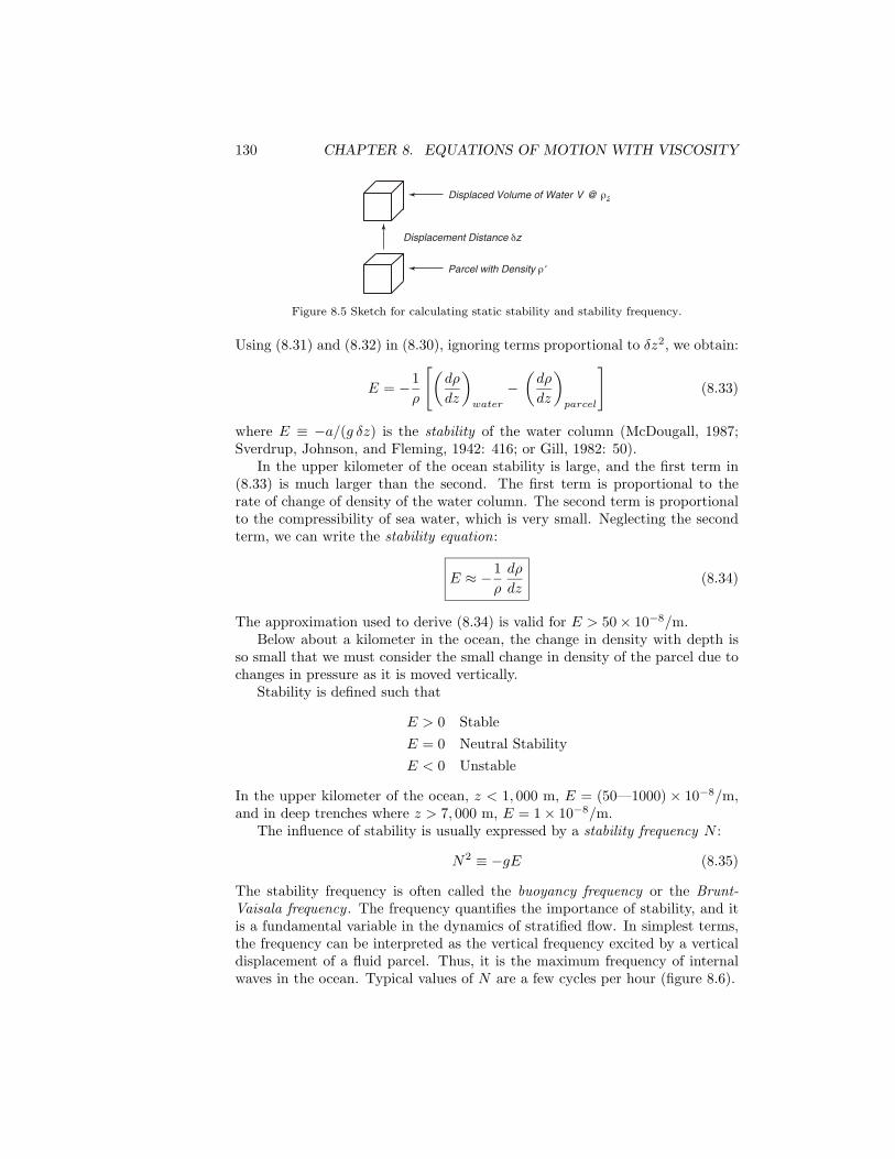
130 CHAPTER 8. EQUATIONS OF MOTION WITH VISCOSITY
Displaced Volume of Water V @ ρ2
Displacement Distance δz
Parcel with Density ρ'
Figure 8.5 Sketch for calculating static stability and stability frequency.
Using (8.31) and (8.32) in (8.30), ignoring terms proportional to δz2, we obtain:
E = −1ρ
[(dρ
dz
)water
−(
dρ
dz
)parcel
](8.33)
where E ≡ −a/(g δz) is the stability of the water column (McDougall, 1987;Sverdrup, Johnson, and Fleming, 1942: 416; or Gill, 1982: 50).
In the upper kilometer of the ocean stability is large, and the first term in(8.33) is much larger than the second. The first term is proportional to therate of change of density of the water column. The second term is proportionalto the compressibility of sea water, which is very small. Neglecting the secondterm, we can write the stability equation:
E ≈ −1ρ
dρ
dz(8.34)
The approximation used to derive (8.34) is valid for E > 50 × 10−8/m.Below about a kilometer in the ocean, the change in density with depth is
so small that we must consider the small change in density of the parcel due tochanges in pressure as it is moved vertically.
Stability is defined such that
E > 0 StableE = 0 Neutral StabilityE < 0 Unstable
In the upper kilometer of the ocean, z < 1, 000 m, E = (50—1000) × 10−8/m,and in deep trenches where z > 7, 000 m, E = 1 × 10⁻⁸/m.
The influence of stability is usually expressed by a stability frequency N :
N2 ≡ −gE (8.35)
The stability frequency is often called the buoyancy frequency or the Brunt-Vaisala frequency . The frequency quantifies the importance of stability, and itis a fundamental variable in the dynamics of stratified flow. In simplest terms,the frequency can be interpreted as the vertical frequency excited by a verticaldisplacement of a fluid parcel. Thus, it is the maximum frequency of internalwaves in the ocean. Typical values of N are a few cycles per hour (figure 8.6).

8.5. STABILITY 131
7.5° N, 137.0° E16 June 1974
35.0° N, 151.9° E24 April 1976
0
1000
2000
3000
40000 1 2 3
Dep
th (
deci
bars
)
-0
-100
-200
-300
-4000 5 10 15
Stability Frequency (cycles per hour)
Figure 8.6. Observed stability frequency in the Pacific. Left: Stability of the deepthermocline east of the Kuroshio. Right: Stability of a shallow thermocline typical of thetropics. Note the change of scales.
Dynamic Stability and Richardson’s Number If velocity changes withdepth in a stable, stratified flow, then the flow may become unstable if thechange in velocity with depth, the current shear , is large enough. The simplestexample is wind blowing over the ocean. In this case, stability is very large acrossthe sea surface. We might say it is infinite because there is a step discontinuityin ρ, and (8.35) is infinite. Yet, wind blowing on the ocean creates waves, and ifthe wind is strong enough, the surface becomes unstable and the waves break.
This is an example of dynamic instability in which a stable fluid is madeunstable by velocity shear. Another example of dynamic instability, the Kelvin-Helmholtz instability, occurs when the density contrast in a sheared flow is muchless than at the sea surface, such as in the thermocline or at the top of a stable,atmospheric boundary layer (figure 8.7).
The relative importance of static stability and dynamic instability is ex-pressed by the Richardson Number :
Ri ≡g E
(∂U/∂z)2(8.36)
where the numerator is the strength of the static stability, and the denominatoris the strength of the velocity shear.
Ri > 0.25 StableRi < 0.25 Velocity Shear Enhances Turbulence
Note that a small Richardson number is not the only criterion for instability.The Reynolds number must be large and the Richardson number must be lessthan 0.25 for turbulence. These criteria are met in some oceanic flows. Theturbulence mixes fluid in the vertical, leading to a vertical eddy viscosity andeddy diffusivity. Because the ocean tends to be strongly stratified and currentstend to be weak, turbulent mixing is intermittent and rare. Measurements of

132 CHAPTER 8. EQUATIONS OF MOTION WITH VISCOSITY
Figure 8.7 Billow clouds showing a Kelvin-Helmholtz instability at the top of a stableatmospheric layer. Some billows can become large enough that more dense air overlies lessdense air, and then the billows collapse into turbulence. Photography copyright BrooksMartner, noaa Environmental Technology Laboratory.
density as a function of depth rarely show more dense fluid over less dense fluidas seen in the breaking waves in figure 8.7 (Moum and Caldwell 1985).
Double Diffusion and Salt Fingers In some regions of the ocean, less densewater overlies more dense water, yet the water column is unstable even if thereare no currents. The instability occurs because the molecular diffusion of heatis about 100 times faster than the molecular diffusion of salt. The instabilitywas first discovered by Melvin Stern in 1960 who quickly realized its importancein oceanography.
Warm, Salty ρ1
Cold, Less Salty ρ2
Warm, Salty ρ1
Cold, Salty ρ > ρ2
Cold, Less Salty ρ2
Initial Density Density after a few minutes
Figure 8.8 Left: Initial distribution of density in the vertical. Right: After some time, thediffusion of heat leads to a thin unstable layer between the two initially stable layers. Thethin unstable layer sinks into the lower layer as salty fingers. The vertical scale in the figuresis a few centimeters.
Consider two thin layers a few meters thick separated by a sharp interface(figure 8.8). If the upper layer is warm and salty, and if the lower is colder andless salty than the upper layer, the interface becomes unstable even if the upperlayer is less dense than the lower.
Here’s what happens. Heat diffuses across the interface faster than salt,leading to a thin, cold, salty layer between the two initial layers. The coldsalty layer is more dense than the cold, less-salty layer below, and the water inthe layer sinks. Because the layer is thin, the fluid sinks in fingers 1–5 cm in

8.6. IMPORTANT CONCEPTS 133
diameter and 10s of centimeters long, not much different in size and shape fromour fingers. This is salt fingering . Because two constituents diffuse across theinterface, the process is called double diffusion.
There are four variations on this theme. Two variables taken two at a timeleads to four possible combinations:
1. Warm salty over colder less salty. This process is called salt fingering. Itoccurs in central waters of sub-tropical gyres, western tropical North At-lantic, and the North-east Atlantic beneath the outflow from the Mediter-ranean Sea. Salt fingering eventually leads to density increasing withdepth in a series of steps. Layers of constant-density are separated bythin layers with large changes in density, and the profile of density as afunction of depth looks like stair steps. Schmitt et al (1987) observed 5–30m thick steps in the western, tropical North Atlantic that were coherentover 200–400 km and that lasted for at least eight months. Kerr (2002)reports a recent experiment by Raymond Schmitt, James Leswell, JohnToole, and Kurt Polzin showed salt fingering off Barbados mixed water 10times faster than turbulence.
2. Colder less salty over warm salty. This process is called diffusive convec-tion. It is much less common than salt fingering, and it us mostly foundat high latitudes. Diffusive convection also leads to a stair step of densityas a function of depth. Here’s what happens in this case. Double diffusionleads to a thin, warm, less-salty layer at the base of the upper, colder,less-salty layer. The thin layer of water rises and mixes with water in theupper layer. A similar processes occurs in the lower layer where a colder,salty layer forms at the interface. As a result of the convection in theupper and lower layers, the interface is sharpened. Any small gradientsof density in either layer are reduced. Neal et al (1969) observed 2–10 mthick layers in the sea beneath the Arctic ice.
3. Cold salty over warmer less salty. Always statically unstable.
4. Warmer less salty over cold salty. Always stable and double diffusiondiffuses the interface between the two layers.
Double diffusion mixes ocean water, and it cannot be ignored. Merryfieldet al (1999), using a numerical model of the ocean circulation that includeddouble diffusion, found that double-diffusive mixing changed the regional distri-butions of temperature and salinity although it had little influence on large-scalecirculation of the ocean.
8.6 Important Concepts1. Friction in the ocean is important only over distances of a few millimeters.
For most flows, friction can be ignored.
2. The ocean is turbulent for all flows whose typical dimension exceeds afew centimeters, yet the theory for turbulent flow in the ocean is poorlyunderstood.

134 CHAPTER 8. EQUATIONS OF MOTION WITH VISCOSITY
3. The influence of turbulence is a function of the Reynolds number of theflow. Flows with the same geometry and Reynolds number have the samestreamlines.
4. Oceanographers assume that turbulence influences flows over distancesgreater than a few centimeters in the same way that molecular viscosityinfluences flow over much smaller distances.
5. The influence of turbulence leads to Reynolds stress terms in the momen-tum equation.
6. The influence of static stability in the ocean is expressed as a frequency,the stability frequency. The larger the frequency, the more stable thewater column.
7. The influence of shear stability is expressed through the Richardson num-ber. The greater the velocity shear, and the weaker the static stability,the more likely the flow will become turbulent.
8. Molecular diffusion of heat is much faster than the diffusion of salt. Thisleads to a double-diffusion instability which modifies the density distribu-tion in the water column in many regions of the ocean.
9. Instability in the ocean leads to mixing. Mixing across surfaces of constantdensity is much smaller than mixing along such surfaces.
10. Horizontal eddy diffusivity in the ocean is much greater than vertical eddydiffusivity.
11. Measurements of eddy diffusivity indicate water is mixed vertically nearoceanic boundaries such as above seamounts and mid-ocean ridges.

Chapter 9
Response of the UpperOcean to Winds
If you have had a chance to travel around the United States, you may havenoticed that the climate of the east coast differs considerably from that on thewest coast. Why? Why is the climate of Charleston, South Carolina so differentfrom that of San Diego, although both are near 32N, and both are on or nearthe ocean? Charleston has 125–150 cm of rain a year, San Diego has 25–50cm, Charleston has hot summers, San Diego has cool summers. Or why is theclimate of San Francisco so different from that of Norfolk, Virginia?
If we look closely at the characteristics of the atmosphere along the twocoasts near 32N, we find more differences that may explain the climate. Forexample, when the wind blows onshore toward San Diego, it brings a cool,moist, marine, boundary layer a few hundred meters thick capped by muchwarmer, dry air. On the east coast, when the wind blows onshore, it brings awarm, moist, marine, boundary layer that is much thicker. Convection, whichproduces rain, is much easier on the east coast than on the west coast. Whythen is the atmospheric boundary layer over the water so different on the twocoasts? The answer can be found in part by studying the ocean’s response tolocal winds, the subject of this chapter.
9.1 Inertial MotionTo begin our study of currents near the sea surface, let’s consider first a verysimple solution to the equations of motion, the response of the ocean to animpulse that sets the water in motion. For example, the impulse can be astrong wind blowing for a few hours. The water then moves only under theinfluence of coriolis force. No other force acts on the water.
Such motion is said to be inertial. The mass of water continues to movedue to its inertia. If the water were in space, it would move in a straight lineaccording to Newton’s second law. But on a rotating earth, the motion is muchdifferent.
135

136 CHAPTER 9. RESPONSE OF THE UPPER OCEAN TO WINDS
From (7.12) the equations of motion for a frictionless ocean are:
du
dt= −1
ρ
∂p
∂x+ 2Ωv sinϕ (9.1a)
dv
dt= −1
ρ
∂p
∂y− 2Ωu sinϕ (9.1b)
dw
dt= −1
ρ
∂p
∂z+ 2Ωu cos ϕ − g (9.1c)
where p is pressure, Ω = 2 π/(sidereal day) = 7.292× 10⁻⁵ rad/s is the rotationof the Earth in fixed coordinates, and ϕ is latitude. We have also used Fi = 0because the fluid is frictionless.
Let’s now look for simple solutions to these equations. To do this we mustsimplify the momentum equations. First, if only the coriolis force acts on thewater, there must be no horizontal pressure gradient:
∂p
∂x=
∂p
∂y= 0
Furthermore, we can assume that the vertical velocity is small, w u, v, so2 Ω cos ϕ g, and (9.1) becomes:
du
dt= 2Ω v sinϕ = fv (9.2a)
dv
dt= −2Ω u sinϕ = −fu (9.2b)
where:
f = 2 Ω sinϕ (9.3)
is the Coriolis Parameter and Ω = 7.292× 10⁻⁵/s is the rotation rate of earth.Equations (9.2) are two coupled, first-order, linear, differential equations
which can be solved with standard techniques. If we solve the second equationfor u, and insert it into the first equation we obtain:
du
dt= − 1
f
d2v
dt2= fv
Rearranging the equation puts it into a standard form we should recognize, theequation for the harmonic oscillator:
d2v
dt2+ f2v = 0 (9.4)
which has the solution (9.5). This current is called an inertial current or inertialoscillation:
u = V sin ftv = V cos ftV 2 = u2 + v2
(9.5)

9.2. EKMAN LAYER AT THE SEA SURFACE 137
100500
km
Inertial Currents
142o 140o 138o 136o
46o
47o
Longitude (West)
Latit
ude
(Nor
th)
Figure 9.1 Inertial currents in the North Pacific in October 1987 (days 275–300) measuredby holey-sock drifting buoys drogued at a depth of 15 meters. Positions were observed 10–12times per day by the Argos system on noaa polar-orbiting weather satellites and interpolatedto positions every three hours. The largest currents were generated by a storm on day277. Note these are not individual eddies. The entire surface is rotating. A drogue placedanywhere in the region would have the same circular motion. After van Meurs (1998).
Note that (9.5) are the parametric equations for a circle with diameter Di =2V/f and period Ti = (2π)/f = Tsd/(2 sinϕ) where Tsd is a sidereal day.
Ti is the inertial period . It is one half the time required for the rotationof a local plane on Earth’s surface (Table 9.1). The rotation is anti-cyclonic:clockwise in the northern hemisphere, counterclockwise in the southern. Inertialcurrents are the free motion of parcels of water on a rotating plane.
Table 9.1 Inertial Oscillations
Latitude (ϕ) Ti (hr) D (km)for V = 20 cm/s
90 11.97 2.735 20.87 4.810 68.93 15.8
Inertial currents are the most common currents in the ocean (figure 9.1).Webster (1968) reviewed many published reports of inertial currents and foundthat currents have been observed at all depths in the ocean and at all latitudes.The motions are transient and decay in a few days. Oscillations at differentdepths or at different nearby sites are usually incoherent.
Inertial currents are caused by rapid changes of wind at the sea surface, withrapid changes of strong winds producing the largest oscillations. Although wehave derived the equations for the oscillation assuming frictionless flow, frictioncannot be completely neglected. With time, the oscillations decay into othersurface currents. (See, for example, Apel, 1987: §6.3 for more information.)
9.2 Ekman Layer at the Sea SurfaceSteady winds blowing on (the sea surface produce a thin, horizontal boundarylayer, the Ekman layer . By thin, I mean a layer that is at most a few-hundredmeters thick, which is thin compared with the depth of the water in the deep

138 CHAPTER 9. RESPONSE OF THE UPPER OCEAN TO WINDS
Table 9.2 Contributions to the Theory of the Wind-Driven Circulation
Fridtjof Nansen (1898) Qualitative theory, currents transport water at anangle to the wind.
Vagn Walfrid Ekman (1902) Quantitative theory for wind-driven transport atthe sea surface.
Harald Sverdrup (1947) Theory for wind-driven circulation in the easternPacific.
Henry Stommel (1948) Theory for westward intensification of wind-drivencirculation (western boundary currents).
Walter Munk (1950) Quantitative theory for main features of the wind-driven circulation.
Kirk Bryan (1963) Numerical models of the oceanic circulation.Bert Semtner (1988) Global, eddy-resolving, realistic model of theand Robert Chervin ocean’s circulation.
ocean. A similar boundary layer exists at the bottom of the ocean, the bottomEkman layer , and at the bottom of the atmosphere just above the sea surface,the planetary boundary layer or frictional layer described in §4.3. The Ekmanlayer is named after Professor Walfrid Ekman, who worked out its dynamics forhis doctoral thesis.
Ekman’s work was the first of a remarkable series of studies conducted duringthe first half of the twentieth century that led to an understanding of how windsdrive the ocean’s circulation (Table 9.1). In this chapter we consider Nansenand Ekman’s work. The rest of the story is given in chapters 11 and 13.
Nansen’s Qualitative Arguments Fridtjof Nansen noticed that wind tendedto blow ice at an angle of 20–40 to the right of the wind in the Arctic, bywhich he meant that the track of the iceberg was to the right of the wind lookingdownwind (See figure 9.2). He later worked out the balance of forces that mustexist when wind tried to push icebergs downwind on a rotating earth.
Nansen argued that three forces must be important:
1. Wind Stress, W;
2. Friction F (otherwise the iceberg would move as fast as the wind);
3. Coriolis Force, C.
Nansen argued further that the forces must have the following attributes:
1. Drag must be opposite the direction of the ice’s velocity;
2. Coriolis force must be perpendicular to the velocity;
3. The forces must balance for steady flow.
W + F + C = 0
Ekman’s Solution Nansen asked Vilhelm Bjerknes to let one of Bjerknes’students make a theoretical study of the influence of Earth’s rotation on wind-driven currents. Walfrid Ekman was chosen, and he presented the results inhis thesis at Uppsala. Ekman later expanded the study to include the influence
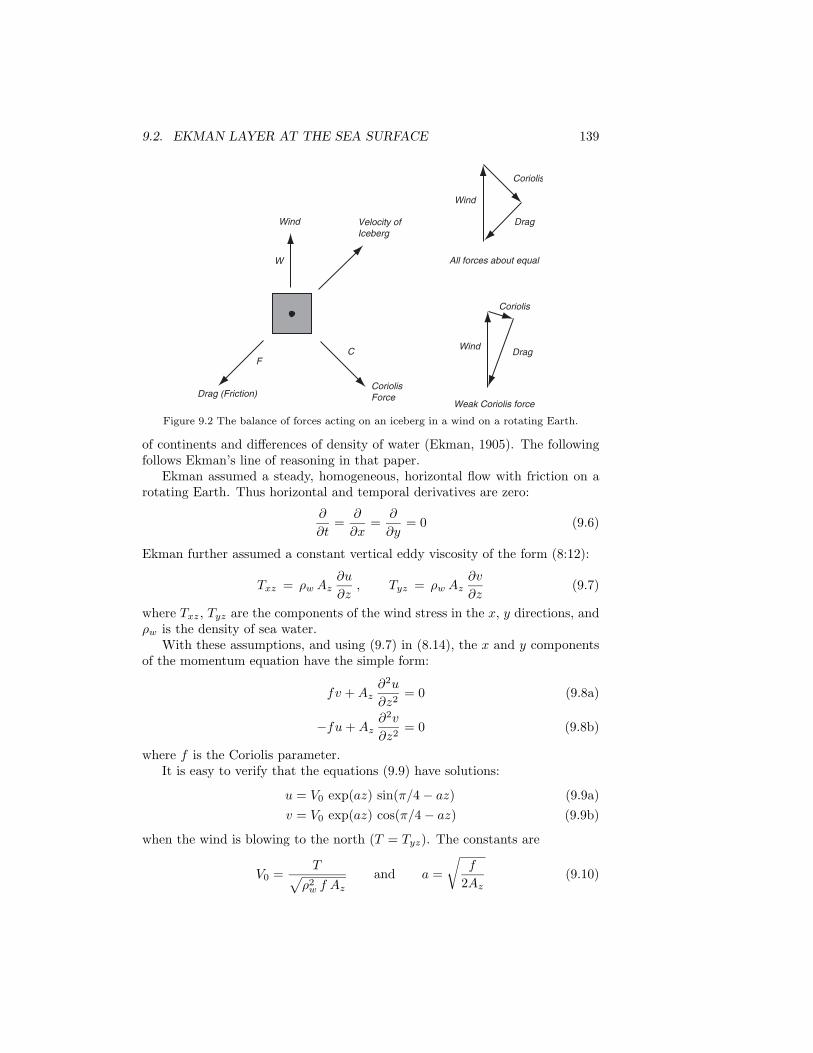
9.2. EKMAN LAYER AT THE SEA SURFACE 139
Wind
W
Velocity ofIceberg
CoriolisForceDrag (Friction)
FC
Coriolis
Drag
Wind
Coriolis
DragWind
All forces about equal
Weak Coriolis force
Figure 9.2 The balance of forces acting on an iceberg in a wind on a rotating Earth.
of continents and differences of density of water (Ekman, 1905). The followingfollows Ekman’s line of reasoning in that paper.
Ekman assumed a steady, homogeneous, horizontal flow with friction on arotating Earth. Thus horizontal and temporal derivatives are zero:
∂
∂t=
∂
∂x=
∂
∂y= 0 (9.6)
Ekman further assumed a constant vertical eddy viscosity of the form (8:12):
Txz = ρw Az∂u
∂z, Tyz = ρw Az
∂v
∂z(9.7)
where Txz, Tyz are the components of the wind stress in the x, y directions, andρw is the density of sea water.
With these assumptions, and using (9.7) in (8.14), the x and y componentsof the momentum equation have the simple form:
fv + Az∂2u
∂z2= 0 (9.8a)
−fu + Az∂2v
∂z2= 0 (9.8b)
where f is the Coriolis parameter.It is easy to verify that the equations (9.9) have solutions:
u = V0 exp(az) sin(π/4 − az) (9.9a)v = V0 exp(az) cos(π/4 − az) (9.9b)
when the wind is blowing to the north (T = Tyz). The constants are
V0 =T√
ρ2w f Az
and a =√
f
2Az(9.10)

140 CHAPTER 9. RESPONSE OF THE UPPER OCEAN TO WINDS
and V0 is the velocity of the current at the sea surface.Now let’s look at the form of the solutions. At the sea surface z = 0,
exp(z = 0) = 1, and
u(0) = V0 cos(π/4) (9.11a)v(0) = V0 sin(π/4) (9.11b)
The current has a speed of V0 to the northeast. In general, the surface current is45 to the right of the wind when looking downwind in the northern hemisphere.The current is 45 to the left of the wind in the southern hemisphere. Belowthe surface, the velocity decays exponentially with depth (figure 9.3):
[u2(z) + v2(z)
]1/2= V0 exp(az) (9.12)
0
-20
-40
-60
-80
-100
-120
-140
Dep
th (
m)
Wind Direction
45o
Vo = 6.4 cm/s
Figure 9.3. Ekman current generated by a 10 m/s wind at 35 N.
Values for Ekman’s Constants To proceed further, we need values for anytwo of the free parameters: the velocity at the surface, V0; the coefficient ofeddy viscosity; Az; or the wind stress T .
The wind stress is well known, and Ekman used the bulk formula (4.2):
Tyz = T = ρair CD U210 (9.13)
where ρair is the density of air, CD is the drag coefficient, and U10 is the windspeed at 10 m above the sea. Ekman turned to the literature to obtain values

9.2. EKMAN LAYER AT THE SEA SURFACE 141
for V0 as a function of wind speed. He found:
V0 =0.0127√sin |ϕ|
U10, |ϕ| ≥ 10 (9.14)
With this information, he could then calculate the velocity as a function ofdepth knowing the wind speed U10 and wind direction.
Ekman Layer Depth The thickness of the Ekman layer is arbitrary becausethe Ekman currents decrease exponentially with depth. Ekman proposed thatthe thickness be the depth DE at which the current velocity is opposite thevelocity at the surface, which occurs at a depth DE = π/a, and the Ekmanlayer depth is:
DE =
√2π2 Az
f(9.15)
Using (9.13) in (9.10), dividing by U10, and using (9.14) and (9.15) gives:
DE =7.6√sin |ϕ|
U10 (9.16)
in SI units. Wind in meters per second gives depth in meters. The constant in(9.16) is based on ρw = 1027 kg/m3, ρair = 1.25 kg/m3, and Ekman’s value ofCD = 2.6 × 10⁻³ for the drag coefficient.
Using (9.16) with typical winds, the depth of the Ekman layer varies fromabout 45 to 300 meters (Table 9.3), and the velocity of the surface current variesfrom 2.5% to 1.1% of the wind speed depending on latitude.
Table 9.3 Typical Ekman Depths
LatitudeU10 [m/s] 15 45
5 75 m 45 m10 150 m 90 m20 300 m 180 m
The Ekman Number: Coriolis and Frictional Forces The depth of theEkman layer is closely related to the depth at which frictional force is equal tothe Coriolis force in the momentum equation (9.9). The Coriolis force is fu,and the frictional force is Az∂
2U/∂z2. The ratio of the forces, which is nondimensional, is called the Ekman Number Ez:
Ez =Friction ForceCoriolis Force
=Az
∂2u
∂z2
fu=
Azu
d2
fu
Ez =Az
f d2(9.17)

142 CHAPTER 9. RESPONSE OF THE UPPER OCEAN TO WINDS
where we have approximated the terms using typical velocities u, and typicaldepths d. The subscript z is needed because the ocean is stratified and mixingin the vertical is much less than mixing in the horizontal. Note that as depthincreases, friction becomes small, and eventually, only the Coriolis force remains.
Solving (9.17) for d gives
d =
√Az
fEz(9.18)
which agrees with the functional form (9.15) proposed by Ekman. Equating(9.18) and (9.15) requires Ez = 1/(2π2) = 0.05 at the Ekman depth. Thus Ek-man chose a depth at which frictional forces are much smaller than the Coriolisforce.
Bottom Ekman Layer The Ekman layer at the bottom of the ocean andthe atmosphere differs from the layer at the ocean surface. The solution for abottom layer below a fluid with velocity U in the x-direction is:
u = U [1 − exp(−az) cos az] (9.19a)v = U exp(−az) sin az (9.19b)
The velocity goes to zero at the boundary, u = v = 0 at z = 0. The directionof the flow close to the boundary is 45 to the left of the flow U outside theboundary layer in the northern hemisphere, and the direction of the flow rotateswith distance above the boundary (figure 9.4). The direction of rotation is anti-cyclonic with distance above the bottom.
Winds above the planetary boundary layer are perpendicular to the pressuregradient in the atmosphere and parallel to lines of constant surface pressure.Winds at the surface are 45 to the left of the winds aloft, and surface currentsare 45 to the right of the wind at the surface. Therefore we expect currentsat the sea surface to be nearly in the direction of winds above the planetaryboundary layer and parallel to lines of constant pressure. Observations of surfacedrifters in the Pacific tend to confirm the hypothesis (figure 9.5).
4
04 8 12
u (m/s)
v (m
/s)
200 300
600
1000
30 305
610
910
100
0 16
Figure 9.4 Ekman layer in the lowest kilometer of the atmosphere (solid line), with windvelocity measured by Dobson (1914) - - - . The numbers give height above the surface inmeters. The Ekman layer at the sea floor has a similar shape. After Houghton (1977: 107).

9.2. EKMAN LAYER AT THE SEA SURFACE 143
60o
50o
40o
30o
20o
10o
0o
-10o
120o 140o 160o 180o -160o -140o -120o -100o
Mean Sea Level Pressure in April 1978 (mb)
1010
1010
1010
55
5
5
5
4
4
4
44
4
4
3
33
3
3
3
6
6
6
6
35
46 5
45
6 6
4 65
55 5
543 6
3
54
3 45 6
34
3 56
6
5
4
43 5
6
543
5 54
6
3
6
6
1015
1015
1012.5
1012.5
1012.5
1017.5
1012.5
Figure 9.5 Trajectories of surface drifters in April 1978 together with surface pressure inthe atmosphere averaged for the month. Note that drifters tend to follow lines of constantpressure except in the Kuroshio where ocean currents are fast compared with velocities inthe Ekman layer in the ocean. After McNally et al. (1983).
Examining Ekman’s Assumptions Before considering the validity of Ek-man’s theory for describing flow in the surface boundary layer of the ocean,let’s first examine the validity of Ekman’s assumptions. He assumed:
1. No boundaries. This is valid away from coasts.
2. Deep water. This is valid if depth 200 m.
3. f -plane. This is valid.
4. Steady state. This is valid if wind blows for longer than a pendulum day.Note however that Ekman also calculated a time-dependent solution, asdid Hasselmann (1970).
5. Az is a function of U210 only. It is assumed to be independent of depth.
This is not a good assumption. The mixed layer may be thinner than theEkman depth, and Az will change rapidly at the bottom of the mixed layerbecause mixing is a function of stability. Mixing across a stable layer ismuch less than mixing through a layer of a neutral stability. More realisticprofiles for the coefficient of eddy viscosity as a function of depth changethe shape of the calculated velocity profile. We reconsider this problembelow.
6. Homogeneous density. This is probably good, except as it effects stability.

144 CHAPTER 9. RESPONSE OF THE UPPER OCEAN TO WINDS
Observations of Flow Near the Sea Surface Does the flow close to thesea surface agree with Ekman’s theory? Measurements of currents made duringseveral, very careful experiments indicate that Ekman’s theory is remarkablygood. The theory accurately describes the flow averaged over many days.
Weller and Plueddmann (1996) measured currents from 2 m to 132 m us-ing 14 vector-measuring current meters deployed from the Floating InstrumentPlatform flip in February and March 1990 500 km west of point Conception,California. This was the last of a remarkable series of experiments coordinatedby Weller using instruments on flip.
Davis, DeSzoeke, and Niiler (1981) measured currents from 2 m to 175 musing 19 vector-measuring current meters deployed from a mooring for 19 daysin August and September 1977 at 50N, 145W in the northeast Pacific.
Ralph and Niiler (2000) tracked 1503 drifters drogued to 15 m depth in thePacific from March 1987 to December 1994. Wind velocity was obtained every 6hours from the European Centre for Medium-Range Weather Forecasts ecmwf.
The results of the experiments indicate that:1. Inertial currents are the largest component of the flow.
2. The flow is nearly independent of depth within the mixed layer for pe-riods near the inertial period. Thus the mixed layer moves like a slabat the inertial period. Current shear is concentrated at the top of thethermocline.
3. The flow averaged over many inertial periods is almost exactly that cal-culated from Ekman’s theory. The shear of the Ekman currents extendsthrough the averaged mixed layer and into the thermocline. Ralph andNiiler found:
DE =7.12√sin |ϕ|
U10 (9.20)
V0 =0.0068√sin |ϕ|
U10 (9.21)
The Ekman-layer depth DE is almost exactly that proposed by Ekman(9.16), but the surface current V0 is half his value (9.14).
4. The transport is 90 to the right of the wind in the northern hemisphere.The transport direction agrees well with Ekman’s theory.
Influence of Stability in the Ekman Layer Ralph and Niiler (2000) pointout that Ekman’s choice of an equation for surface currents (9.14), which leadsto (9.16), is consistent with theories that include the influence of stability in theupper ocean. Currents with periods near the inertial period produce shear in thethermocline. The shear mixes the surface layers when the Richardson numberfalls below the critical value (Pollard et al. 1973). This idea, when included inmixed-layer theories, leads to a surface current V0 that is proportional to
√N/f
V0 ∼ U10
√N/f (9.22)

9.3. EKMAN MASS TRANSPORTS 145
furthermore
Az ∼ U210/N and DE ∼ U10/
√Nf (9.23)
Notice that (9.22) and (9.23) are now dimensionally correct. The equations usedearlier, (9.14), (9.16), (9.20), and (9.21) all required a dimensional coefficient.
9.3 Ekman Mass TransportsFlow in the Ekman layer at the sea surface carries mass. For many reasons wemay want to know the total mass transported in the layer. The Ekman transportME is defined as the integral of the Ekman velocity UE , VE from the surface toa depth d below the Ekman layer. The two components of the transport areMEx, MEy :
MEx =∫ 0
−d
ρUE dz, MEy =∫ 0
−d
ρVE dz (9.24)
The transport has units kg/(m·s). It is the mass of water passing througha vertical plane one meter wide that is perpendicular to the transport andextending from the surface to depth −d (figure 9.6).
U U
z
y
QX =
Y MX
r
Y1m
x
Sea Surface
Figure 9.6 Sketch for defining Left: mass transports, and Right: volume transports.
We calculate the Ekman mass transports by integrating (8.14) in (9.24):
f
∫ 0
−d
ρ VE dz = f MEy = −∫ 0
−d
dTxz
f MEy = −Txz
∣∣z=0
+ Txz
∣∣z=−d
(9.25)
A few hundred meters below the surface the Ekman velocities approach zero,and the last term of (9.25) is zero. Thus mass transport is due only to windstress at the sea surface (z = 0). In a similar way, we can calculate the transportin the x direction to obtain the two components of the Ekman transport :
f MEy = −Txz(0) (9.26a)f MEx = Tyz(0) (9.26b)
where Txz(0), Tyz(0) are the two components of the stress at the sea surface.

146 CHAPTER 9. RESPONSE OF THE UPPER OCEAN TO WINDS
Notice that the transport is perpendicular to the wind stress, and to the rightof the wind in the northern hemisphere. If the wind is to the north in the positivey direction (a south wind), then Txz(0) = 0, MEy = 0, and MEx = Tyz(0)/f .In the northern hemisphere, f is positive, and the mass transport is in the xdirection, to the east.
It may seem strange that the drag of the wind on the water leads to a currentat right angles to the drag. The result follows from the assumption that frictionis confined to a thin surface boundary layer, that it is zero in the interior ofthe ocean, and that the current is in equilibrium with the wind so that it is nolonger accelerating.
Volume transport Q is the mass transport divided by the density of waterand multiplied by the width perpendicular to the transport.
Qx =Y Mx
ρ, Qy =
XMy
ρ(9.27)
where Y is the north-south distance across which the eastward transport Qx iscalculated, and X in the east-west distance across which the northward trans-port Qy is calculated. Volume transport has dimensions of cubic meters persecond. A convenient unit for volume transport in the ocean is a million cubicmeters per second. This unit is called a Sverdrup, and it is abbreviated Sv.
Recent observations of Ekman transport in the ocean agree with the the-oretical values (9.26). Chereskin and Roemmich (1991) measured the Ekmanvolume transport across 11N in the Atlantic using an acoustic Doppler cur-rent profiler described in Chapter 10. They calculated a southward transportQy = 12.0±5.5 Sv from direct measurements of current, Qy = 8.8±1.9 Sv frommeasured winds using (9.26) and (9.27), and Qy = 13.5 ± 0.3 Sv from meanwinds averaged over many years at 11N.
Use of Transports Mass transports are widely used for two important rea-sons. First, the calculation is much more robust than calculations of velocitiesin the Ekman layer. By robust, I mean that the calculation is based on fewerassumptions, and that the results are more likely to be correct. Thus the cal-culated mass transport does not depend on knowing the distribution of velocityin the Ekman layer or the eddy viscosity.
Second, the variability of transport in space has important consequences.Let’s look at a few applications.
9.4 Application of Ekman TheoryBecause steady winds blowing on the sea surface produce an Ekman layer thattransports water at right angles to the wind direction, any spatial variabilityof the wind, or winds blowing along some coasts, can lead to upwelling. Andupwelling is important:
1. Upwelling enhances biological productivity, which feeds fisheries.2. Cold upwelled water alters local weather. Weather onshore of regions of
upwelling tend to have fog, low stratus clouds, a stable stratified atmo-sphere, little convection, and little rain.

9.4. APPLICATION OF EKMAN THEORY 147
Upwelling Water
ME
ME 100 - 300 m
Col
dU
pwel
led
Wat
er
Win
dLand
(California)
Ekman Transport
100 km
Figure 9.7 Sketch of Ekman transport along a coast leading to upwelling of cold water alongthe coast. Left: Cross section. The water transported offshore must be replaced by waterupwelling from below the mixed layer. Right: Plan view. North winds along a west coast inthe northern hemisphere cause Ekman transports away from the shore.
3. Spatial variability of transports in the open ocean leads to upwelling anddownwelling, which leads to redistribution of mass in the ocean, whichleads to wind-driven geostrophic currents via Ekman pumping.
Coastal Upwelling To see how winds lead to upwelling, consider north windsblowing parallel to the California Coast (figure 9.7 left). The winds producea mass transport away from the shore everywhere along the shore. The waterpushed offshore can be replaced only by water from below the Ekman layer.This is upwelling (figure 9.7 right). Because the upwelled water is cold, theupwelling leads to a region of cold water at the surface along the coast. Figure10.16 shows the distribution of cold water off the coast of California.
Upwelled water is colder than water normally found on the surface, andit is richer in nutrients. The nutrients fertilize phytoplankton in the mixedlayer, which are eaten by zooplankton, which are eaten by small fish, whichare eaten by larger fish and so on to infinity. As a result, upwelling regionsare productive waters supporting the world’s major fisheries. The importantregions are offshore of Peru, California, Somalia, Morocco, and Namibia.
Now we can answer the question we asked at the beginning of the chapter:Why is the climate of San Francisco so different from that of Norfolk, Virginia?Figures 4.2 or 9.7 show that wind along the California and Oregon coasts has astrong southward component. The wind causes upwelling along the coast, whichleads to cold water close to shore. The shoreward component of the wind bringswarmer air from far offshore over the colder water, which cools the incomingair close to the sea, leading to a thin, cool atmospheric boundary layer. As theair cools, fog forms along the coast. Finally, the cool layer of air is blown overSan Francisco, cooling the city. The warmer air above the boundary layer, dueto downward velocity of the Hadley circulation in the atmosphere (see figure4.3), inhibits vertical convection, and rain is rare. Rain forms only when winterstorms coming ashore bring strong convection higher up in the atmosphere.
In addition to upwelling, other processes influence weather in California andVirginia.

148 CHAPTER 9. RESPONSE OF THE UPPER OCEAN TO WINDS
1. The oceanic mixed layer tends to be thin on the eastern side of oceans,and upwelling can easily bring up cold water.
2. Currents along the eastern side of oceans at mid-latitudes tend to bringcolder water from higher latitudes.
All these processes are reversed offshore of east coasts, leading to warm waterclose to shore, thick atmospheric boundary layers, and frequent convective rain.Thus Norfolk is much different that San Francisco due to upwelling and thedirection of the coastal currents.
Ekman Pumping The horizontal variability of the wind blowing on the seasurface leads to horizontal variability of the Ekman transports. Because massmust be conserved, the spatial variability of the transports must lead to verticalvelocities at the top of the Ekman layer. To calculate this velocity, we firstintegrate the continuity equation (7.19) in the vertical:
ρ
∫ 0
−d
(∂u
∂x+
∂v
∂y+
∂w
∂z
)dz = 0
∂
∂x
∫ 0
−d
ρ u dz +∂
∂y
∫ 0
−d
ρ v dz = −ρ
∫ 0
−d
∂w
∂zdz
∂MEx
∂x+
∂MEy
∂y= −ρ [w(0) − w(−d)] (9.28)
By definition, the Ekman velocities approach zero at the base of the Ekmanlayer, and the vertical velocity at the base of the layer wE(−d) due to divergenceof the Ekman flow must be zero. Therefore:
∂MEx
∂x+
∂MEy
∂y= −ρ wE(0) (9.29a)
∇H · ME = −ρ wE(0) (9.29b)
Where ME is the vector mass transport due to Ekman flow in the upper bound-ary layer of the ocean, and ∇H is the horizontal divergence operator. (9.29)states that the horizontal divergence of the Ekman transports leads to a verti-cal velocity in the upper boundary layer of the ocean, a process called EkmanPumping .
If we use the Ekman mass transports (9.26) in (9.29) we can relate Ekmanpumping to the wind stress.
wE(0) = −1ρ
[∂
∂x
(Tyz(0)
f
)− ∂
∂y
(Txz(0)
f
)](9.30a)
wE(0) = −curl(
Tρ f
)(9.30b)
where T is the vector wind stress.

9.5. LANGMUIR CIRCULATION 149
The vertical velocity at the sea surface w(0) must be zero because the surfacecannot rise into the air, so wE(0) must be balanced by another vertical velocity.We will see in Chapter 12 that it is balanced by a geostrophic velocity wG(0)at the top of the interior flow in the ocean.
Note that the derivation above follows Pedlosky (1996: 13), and it differsfrom the traditional approach that leads to a vertical velocity at the base of theEkman layer. Pedlosky points out that if the Ekman layer is very thin comparedwith the depth of the ocean, it makes no difference whether the velocity iscalculated at the top or bottom of the Ekman layer, but this is usually not truefor the ocean. Hence, we must compute vertical velocity at the top of the layer.
9.5 Langmuir CirculationMeasurements of surface currents show that winds generate more than Ekmanand inertial currents at the sea surface. They also generate a Langmuir circula-tion (Langmuir, 1938), a current that spiral around an axis parallel to the winddirection. Weller et al. (1985) observed such a flow during an experiment tomeasure the wind-driven circulation in the upper 50 meters of the sea. Theyfound that during a period when the wind speed was 14 m/s, surface currentswere organized into Langmuir cells spaced 20 m apart, the cells were aligned atan angle of 15 to the right of the wind, and vertical velocity at 23 m depth wasconcentrated in narrow jets under the areas of surface convergence (figure 9.8).
-10
-20
10
V
10
10
20
0
WU
T
Figure 9.8 A three-dimensional view of the Langmuir circulation at the surface of the Pacificobserved from the Floating Instrument Platform flip. The heavy dashed line on the seasurface indicate lines of convergence marked by cards on the surface. Vertical arrows areindividual values of vertical velocity measured every 14 seconds at 23 m depth as the platformdrifted through the Langmuir currents. Horizontal arrows, which are drawn on the surfacefor clarity, are values of horizontal velocity at 23 m. The broad arrow gives the direction ofthe wind. After Weller et al. (1985).

150 CHAPTER 9. RESPONSE OF THE UPPER OCEAN TO WINDS
Maximum vertical velocity was −0.18 m/s. The seasonal thermocline was at 50m, and no downward velocity was observed in or below the thermocline.
9.6 Important Concepts1. Changes in wind stress produce transient oscillations in the ocean called
inertial currents
(a) Inertial currents are very common in the ocean.(b) The period of the current is (2π)/f .
2. Steady winds produce a thin boundary layer, the Ekman layer, at the topof the ocean. Ekman boundary layers also exist at the bottom of the oceanand the atmosphere. The Ekman layer in the atmosphere above the seasurface is called the planetary boundary layer.
3. The Ekman layer at the sea surface has the following characteristics:
(a) Direction: 45to the right of the wind looking downwind in theNorthern Hemisphere.
(b) Surface Speed : 1–2.5% of wind speed depending on latitude.(c) Depth: approximately 40–300 m depending on latitude and wind
velocity.
4. Careful measurements of currents near the sea surface show that:
(a) Inertial oscillations are the largest component of the current in themixed layer.
(b) The flow is nearly independent of depth within the mixed layer forperiods near the inertial period. Thus the mixed layer moves like aslab at the inertial period.
(c) An Ekman layer exists in the atmosphere just above the sea (andland) surface.
(d) Surface drifters tend to drift parallel to lines of constant atmosphericpressure at the sea surface. This is consistent with Ekman’s theory.
(e) The flow averaged over many inertial periods is almost exactly thatcalculated from Ekman’s theory.
5. Transport is 90 to the right of the wind in the northern hemisphere.
6. Spatial variability of Ekman transport, due to spatial variability of windsover distances of hundreds of kilometers and days, leads to convergenceand divergence of the transport.
(a) Winds blowing toward the equator along west coasts of continentsproduces upwelling along the coast. This leads to cold, productivewaters within about 100 km of the shore.
(b) Upwelled water along west coasts of continents modifies the weatheralong the west coasts.
7. Ekman pumping, which is driven by spatial variability of winds, drivesa vertical current, which drives the interior geostrophic circulation of theocean.

Chapter 10
Geostrophic Currents
Within the ocean’s interior away from the top and bottom Ekman layers, forhorizontal distances exceeding a few tens of kilometers, and for times exceedinga few days, horizontal pressure gradients in the ocean almost exactly balancethe Coriolis force resulting from horizontal currents. This balance is known asthe geostrophic balance.
The dominant forces acting in the vertical are the vertical pressure gradientand the weight of the water. The two balance within a few parts per million.Thus pressure at any point in the water column is due almost entirely to theweight of the water in the column above the point. The dominant forces in thehorizontal are the pressure gradient and the Coriolis force. They balance withina few parts per thousand over large distances and times (See Box).
Both balances require that viscosity and nonlinear terms in the equationsof motion be negligible. Is this reasonable? Consider viscosity. We know thata rowboat weighing a hundred kilograms will coast for maybe ten meters afterthe rower stops. A super tanker moving at the speed of a rowboat may coastfor kilometers. It seems reasonable, therefore that a cubic kilometer of waterweighing 1015 kg would coast for perhaps a day before slowing to a stop. Andoceanic mesoscale eddies contain perhaps 1000 cubic kilometers of water. Hence,our intuition may lead us to conclude that neglect of viscosity is reasonable. Ofcourse, intuition can be wrong, and we need to refer back to scaling arguments.
10.1 Hydrostatic EquilibriumBefore describing the geostrophic balance, let’s first consider the simplest solu-tion of the momentum equation, the solution for an ocean at rest. It gives thehydrostatic pressure within the ocean. To obtain the solution, we assume thefluid is stationary:
u = v = w = 0; (10.1)
the fluid remains stationary:du
dt=
dv
dt=
dw
dt= 0; (10.2)
151

152 CHAPTER 10. GEOSTROPHIC CURRENTS
Scaling the Equations: The Geostrophic Approximation
We wish to simplify the equations of motion to obtain solutions that describe thedeep-sea conditions well away from coasts and below the Ekman boundary layer atthe surface. To begin, let’s examine the typical size of each term in the equationsin the expectation that some will be so small that they can be dropped withoutchanging the dominant characteristics of the solutions. For interior, deep-seaconditions, typical values for distance L, horizontal velocity U , depth H, Coriolisparameter f , gravity g, and density ρ are:
L ≈ 106 m f ≈ 10−4 s−1
U ≈ 10−1 m/s g ≈ 10 m/s2
H ≈ 103 m ρ ≈ 103 kg/m3
From these variables we can calculate typical values for vertical velocity W ,pressure P , and time T :
∂W
∂z= −
(∂U
∂x+
∂v
∂y
)W
H=
U
L; W =
UH
L=
10−1 103
106m/s = 10−4m/s
P = ρgz = 103 101 103 = 107 Pa
T = L/U = 107 s
The momentum equation for vertical velocity is therefore:
∂w
∂t+ u
∂w
∂x+ v
∂w
∂y+ w
∂w
∂z= −1
ρ
∂p
∂z+ 2Ω u cos ϕ − g
W
T+
UW
L+
UW
L+
W 2
L=
P
ρ H+ f U − g
10−11 + 10−11 + 10−11 + 10−14 = 10 + 10−5 − 10
and the only important balance in the vertical is hydrostatic:
∂p
∂z= −ρg Correct to 1 : 106.
The momentum equation for horizontal velocity in the x direction is:
∂u
∂t+ u
∂u
∂x+ v
∂u
∂y+ w
∂u
∂z= −1
ρ
∂P
∂x+ fv
10−8 + 10−8 + 10−8 + 10−8 = 10−5 + 10−5
Thus the Coriolis force balances the pressure gradient within one part per thou-sand. This is called the geostrophic balance, and the geostrophic equations are:
1
ρ
∂p
∂x= fv;
1
ρ
∂p
∂y= −fu;
1
ρ
∂p
∂z= −g
This balance applies to oceanic flows with horizontal dimensions larger thanroughly 50 km and times greater than a few days.

10.2. GEOSTROPHIC EQUATIONS 153
and, there is no friction:
fx = fy = fz = 0. (10.3)
With these assumptions the momentum equation (7.12) becomes:
1ρ
∂p
∂x= 0;
1ρ
∂p
∂y= 0;
1ρ
∂p
∂z= − g(ϕ, z) (10.4)
where we have explicitly noted that gravity g is a function of latitude ϕ andheight z. We will show later why we have kept this explicit.
Equations (10.4a) require surfaces of constant pressure to be level surface.A surface of constant pressure is an isobaric surface. The last equation can beintegrated to obtain the pressure at any depth h. Recalling that ρ is a functionof depth for an ocean at rest.
p =∫ 0
−h
g(ϕ, z) ρ(z) dz (10.5)
For many purposes, g and ρ are constant, and p = ρ g h. Later, we will showthat (10.5) applies with an accuracy of about one part per million even if theocean is not at rest.
The SI unit for pressure is the pascal (Pa). A bar is another unit of pressure.One bar is exactly 105 Pa (table 10.1). Because the depth in meters and pressurein decibars are almost the same numerically, oceanographers prefer to statepressure in decibars.
Table 10.1 Units of Pressure
1 pascal (Pa) = 1 N/m2 = 1 kg·s−2·m−1
1 bar = 105 Pa1 decibar = 104 Pa1 millibar = 100 Pa
10.2 Geostrophic EquationsThe geostrophic balance requires that the Coriolis force balance the horizontalpressure gradient. The equations for geostrophic balance are derived from theequations of motion assuming the flow has no acceleration, du/dt = dv/dt =dw/dt = 0; that horizontal velocities are much larger than vertical, w u, v;that the only external force is gravity; and that friction is small. With theseassumptions (7.12) become
∂p
∂x= ρfv;
∂p
∂y= −ρfu;
∂p
∂z= −ρg (10.6)
where f = 2Ω sinϕ is the Coriolis parameter. These are the geostrophic equa-tions.
The equations can be written:
u = − 1fρ
∂p
∂y; v =
1fρ
∂p
∂x(10.7a)

154 CHAPTER 10. GEOSTROPHIC CURRENTS
p = p0 +∫ ζ
−h
g(ϕ, z)ρ(z)dz (10.7b)
where p0 is atmospheric pressure at z = 0, and ζ is the height of the sea surface.Note that we have allowed for the sea surface to be above or below the surfacez = 0; and the pressure gradient at the sea surface is balanced by a surfacecurrent us.
Substituting (10.7b) into (10.7a) gives:
u = − 1fρ
∂
∂y
∫ 0
−h
g(ϕ, z) ρ(z) dz − g
f
∂ζ
∂y
u = − 1fρ
∂
∂y
∫ 0
−h
g(ϕ, z) ρ(z) dz − us (10.8a)
where we have used the Boussinesq approximation, retaining full accuracy forρ only when calculating pressure.
In a similar way, we can derive the equation for v.
v =1fρ
∂
∂x
∫ 0
−h
g(ϕ, z) ρ(z) dz +g
f
∂ζ
∂x
v =1fρ
∂
∂x
∫ 0
−h
g(ϕ, z) ρ(z) dz + vs (10.8b)
If the ocean is homogeneous and density and gravity are constant, the firstterm on the right-hand side of (10.8) is equal to zero; and the horizontal pressuregradients within the ocean are the same as the gradient at z = 0. This isbarotropic flow described in §10.4.
If the ocean is stratified, the horizontal pressure gradient has two terms, onedue to the slope at the sea surface, and an additional term due to horizontaldensity differences. These equations include baroclinic flow also discussed in§10.4. The first term on the right-hand side of (10.8) is due to variations indensity ρ(z), and it is called the relative velocity. Thus calculation of geostrophiccurrents from the density distribution requires the velocity (u0, v0) at the seasurface or at some other depth.
1m
100km
z
x
-r
z=-r
0
Sea Surface (z=ζ )
ζ
Figure 10.1 Sketch defining ζ and r, used for calculating pressure just below the sea surface.

10.3. SURFACE GEOSTROPHIC CURRENTS FROM ALTIMETRY 155
10.3 Surface Geostrophic Currents From AltimetryThe geostrophic approximation applied at z = 0 leads to a very simple relation:surface geostrophic currents are proportional to surface slope. Consider a levelsurface slightly below the sea surface, say two meters below the sea surface, atz = −r. A level surface is a surface of constant gravitational potential, and nowork is required to move along a frictionless, level surface (figure 10.1).
The pressure on the level surface is:
p = ρ g (ζ + r) (10.9)
assuming ρ and g are essentially constant in the upper few meters of the ocean.Substituting this into (10.7a, b), gives the two components (us, vs) of the
surface geostrophic current:
us = − g
f
∂ζ
∂y; vs =
g
f
∂ζ
∂x(10.10)
where g is gravity, f is the Coriolis parameter, and ζ is the height of the seasurface above a level surface.
The Oceanic Topography In §3.4 we define the topography of the sea surfaceζ to be the height of the sea surface relative to a particular level surface, thegeoid; and we defined the geoid to be the level surface that coincided with thesurface of the ocean at rest. Thus, according to (10.10) the surface geostrophiccurrents are proportional to the slope of the topography (figure 10.2), a quantitythat can be measured by satellite altimeters if the geoid is known.
z=ζ
Vs =g
f
dζ
dx
Sea Surface
Geoid
Vs 1m
100km
⊗
x
Figure 10.2 The slope of the sea surface relative to the geoid (∂ζ/∂x) is directly related tosurface geostrophic currents vs. The slope of 1 meter per 100 kilometers (10 µrad) is typicalof strong currents. Vs is into the paper in the northern hemisphere.
Because the geoid is a level surface, it is a surface of constant geopoten-tial. To see this, consider the work done in moving a mass m by a distanceh perpendicular to a level surface. The work is W = mgh, and the change ofpotential energy per unit mass is gh. Thus level surfaces are surfaces of constantgeopotential, where the geopotential Φ = gh.
Topography is due to processes that cause the ocean to move: tides, oceancurrents, and the changes in barometric pressure that produce the invertedbarometer effect. Because the ocean’s topography is due to dynamical processes,it is usually called dynamic topography . The topography is approximately onehundredth of the geoid undulations. This means that the shape of the sea surface

156 CHAPTER 10. GEOSTROPHIC CURRENTS
mean sea surface
mean geoid
Gulf Stream
Geoid ErrorCold Core Rings
Warm Core Rings
40o 38o 36o 34o 32o 30o 28o 26o 24o 22o 20o
-0.5
0.0
0.5
1.0
-60
-55
-50
-45
-40
-35
SS
T (
m)
Hei
ght (
m)
North Latitude
Figure 10.3 Topex/Poseidon altimeter observations of the Gulf Stream. When the altimeterobservations are subtracted from the local geoid, they yield the oceanic topography, which isdue primarily to ocean currents in this example. The gravimetric geoid was determined bythe Ohio State University from ship and other surveys of gravity in the region. From Centerfor Space Research, University of Texas.
is dominated by local variations of gravity. The influence of currents is muchsmaller. Typically, sea-surface topography has amplitude of ±1 m. Typicalslopes are ∂ζ/∂x ≈ 1–10 microradians for v = 0.1–1.0 m/s at mid latitude.
Errors in knowing the height of the geoid are larger than the topographyfor features with horizontal extent less than roughly 1600 km (Nerem et al.1994). The height of the geoid, smoothed over horizontal distances greater thanroughly 1,600 km, is known with an accuracy of ±15 cm (Tapley et al. 1994a).The height of the unsmoothed, local geoid is known with an accuracygeoid ofonly around ±50 cm (figure 10.3).
Satellite Altimetry Very accurate, satellite-altimeter systems are needed formeasuring the oceanic topography. The first systems, carried on Seasat, Geosat,ers–1, and ers–2 were designed to measure week-to-week variability of currents.Topex/Poseidon, launched in 1992, was the first satellite designed to make themuch more accurate measurements necessary for observing the permanent (time-averaged) surface circulation of the oceans, tides, and the variability of gyre-scalecurrents. It was replaced in 2001 by Jason.
Because the geoid is not well known locally, altimeters are usually flown inorbits that have an exactly repeating ground track. Thus Topex/Poseidon andJason fly over the same ground track every 9.9156 days. By subtracting sea-surface height from one traverse of the ground track from height measured ona later traverse, changes in topography can be observed without knowing the

10.3. SURFACE GEOSTROPHIC CURRENTS FROM ALTIMETRY 157
15
15
10
8
8
6
6
15
15
1515
Topography Variability (cm)
20o 60o 100o 140o 180o -140o -100o -60o -20o 20o-64o
-32o
0o
32o
64o
15
0o
15
15
Figure 10.4 Global distribution of variance of topography from Topex/Poseidon altimeterdata from 10/3/92 to 10/6/94. The height variance is an indicator of variability of surfacegeostrophic currents. From Center for Space Research, University of Texas.
geoid. The geoid is constant in time, and the subtraction removes the geoid,revealing changes due to changing currents, such as mesoscale eddies, assumingtides have been removed from the data (figure 10.4). Mesoscale variabilityincludes eddies with diameters between roughly 20 and 500 km.
The great accuracy and precision of the Topex/Poseidon and Jason altimetersystems allow them to measure the oceanic topography over ocean basins withan accuracy of ±5 cm. This allows them to measure:
1. Changes in the mean volume of the ocean (Born et al. 1986, Nerem, 1995);2. Seasonal heating and cooling of the ocean (Chambers et al 1998);3. Tides (Andersen, Woodworth, and Flather, 1995);4. The permanent surface geostrophic current system (figure 10.5);5. Changes in surface geostrophic currents on all scales (figure 10.4); and6. Variations in topography of equatorial current systems such as those as-
sociated with El Nino (figure 10.6).
Altimeter Errors (Topex/Poseidon) The most accurate observations of thesea-surface topography are from Topex/Poseidon and Jason. Errors for thesesatellite altimeter system are due to:
1. Instrument noise, ocean waves, water vapor, free electrons in the iono-sphere, and mass of the atmosphere. Topex/Poseidon carries a precisealtimeter system able to observed the height of the satellite above the seasurface between ±66latitude with a precision of ±2 cm and an accuracyof ±3.2 cm (Fu et al. 1994). The system consists of a two-frequency radaraltimeter to measure height above the sea, the influence of the ionosphere,and wave height. The system also included a three-frequency microwaveradiometer able to measure water vapor in the troposphere.

158 CHAPTER 10. GEOSTROPHIC CURRENTS
Four-Year Mean Sea-Surface Topography (cm)
-100-100
-100-150
-150-150
120
0
2040
40404040
0 0
20
202020
-50
120
60
60 60
60
60
80
80
80
80
80
80
100
60
80
40
60
0
60
40
60
404020
40
40
80
-50-100
-150
20o 60o 100o 140o 180o -140o -100o -60o -20o 20o 0o
-66o
-44o
-22o
0o
22o
44o
66o
Figure 10.5 Global distribution of time-averaged topography of the ocean from Topex/Pos-eidon altimeter data from 10/3/92 to 10/6/99 relative to the jgm–3 geoid. Geostrophiccurrents at the ocean surface are parallel to the contours. Compare with figure 2.8 calculatedfrom hydrographic data. From Center for Space Research, University of Texas.
2. Tracking errors. The satellite carries three tracking systems that enableits position in space, its ephemeris, to be determined with an accuracy of±3.5 cm (Tapley et al. 1994b).
3. Sampling error. The satellite measures height along a ground track thatrepeats within ±1 km every 9.9156 days. Each repeat is a cycle. Becausecurrents are measured only along the subsatellite track, there is a samplingerror. The satellite cannot map the topography between ground tracks,nor can it observe changes with periods less than 2× 9.9156 d (see §16.3).
4. Geoid error. The permanent topography is not well known over distancesshorter than 1,600 km because geoid errors dominate for shorter distances.Maps of the topography smoothed over 1,600 km are used to study thedominant features of the permanent geostrophic currents at the sea sur-face (figure 10.5).New satellite systems grace and champ are measuringearth’s gravity with enough accuracy that the geoid error will soon besmall enough to ignore over distances as short as 100 km.
Taken together, the measurements of height above the sea and the satellite po-sition give sea-surface height in geocentric coordinates with an ±4.7 cm. Thegeoid error adds further errors that depend on the size of the area being mea-sured.
10.4 Geostrophic Currents From HydrographyThe geostrophic equations are widely used in oceanography to calculate currentsat depth. The basic idea is to use hydrographic measurements of temperature,salinity or conductivity, and pressure to calculate the density field of the oceanusing the equation of state of sea water. Density is used in (10.7b) to calculate

10.4. GEOSTROPHIC CURRENTS FROM HYDROGRAPHY 159
150
155
160
165
170
175
180
185
190
195
200
205
210
215
220
225
230
235
240
245
250
255
260
265
270
275
280
285
290
295
300
305
310
315
320
140 160 180 200 220 240 260 280
10/9/96
11/28/96
1/16/97
3/7/97
4/25/97
6/14/97
8/3/97
9/21/97
11/10/97
12/29/97
2/17/98
4/7/98
5/27/98
7/16/98
9/3/98
10/23/98
12/11/98
1/30/99
3/20/99
5/9/99
6/28/99
8/4/99
10/5/99
11/23/99
1/22/00
3/2/00
4/20/00
6/9/00
7/28/00
9/16/00
11/4/00
12/24/00
2/12/01
4/2/01
5/22/01
-25 -20 -15 -10 -5 0 5 10 15 20 25 30cm
Figure 10.6 Time-longitude plot of sea-level anomalies in the Equatorial Pacific observedby Topex/Poseidon. Warm anomalies are light gray, cold anomalies are dark gray. Theanomalies are computed from 10-day deviations from a three-year mean surface from 3Oct 1992 to 8 Oct 1995. The data are smoothed with a Gaussian weighted filter with alongitudinal span of 5and a latitudinal span of 2. The annotations on the left are cycles ofsatellite data. From Center for Space Research, University of Texas.

160 CHAPTER 10. GEOSTROPHIC CURRENTS
the internal pressure field, from which the geostrophic currents are calculatedusing (10.8a, b). Usually, however, the constant of integration in (10.8) is notknown, and only the relative velocity field can be calculated.
At this point, you may ask, why not just measure pressure directly as is donein meteorology, where direct measurements of pressure are used to calculatewinds. And, aren’t pressure measurements needed to calculate density fromthe equation of state? The answer is that very small changes in depth makelarge changes in pressure because water is so heavy. Errors in pressure causedby errors in determining the depth of a pressure gauge are much larger thanthe pressure due to currents. For example, using (10.7a), we calculate that thepressure gradient due to a 10 cm/s current at 30latitude is 7.5 × 10⁻³ Pa/m,which is 750 Pa in 100 km. From the hydrostatic equation (10.5), 750 Pa isequivalent to a change of depth of 7.4 cm. Therefore, for this example, we mustknow the depth of a pressure gauge with an accuracy of much better than 7.4cm. This is not possible.
Geopotential Surfaces Within the Ocean Calculation of pressure gradientswithin the ocean must be done along surfaces of constant geopotential just as wecalculated surface pressure gradients relative to the geoid when we calculatedsurface geostrophic currents. As long ago as 1910, Vilhelm Bjerknes (Bjerknesand Sandstrom, 1910) realized that such surfaces are not at fixed heights in theatmosphere because g is not constant, and (10.4) must include the variabilityof gravity in both the horizontal and vertical directions (Saunders and Fofonoff,1976) when calculating pressure in the ocean.
The geopotential Φ is:
Φ =∫ z
0
gdz (10.11)
Because Φ/9.8 in SI units has almost the same numerical value as height in me-ters, the meteorological community accepted Bjerknes’ proposal that height bereplaced by dynamic meters D = Φ/10 to obtain a natural vertical coordinate.Later, this was replaced by the geopotential meter (gpm) Z = Φ/9.80. Thegeopotential meter is a measure of the work required to lift a unit mass fromsea level to a height z against the force of gravity. Harald Sverdrup, Bjerknes’student, carried the concept to oceanography, and depths in the ocean are oftenquoted in geopotential meters. The difference between depths of constant ver-tical distance and constant potential can be relatively large. For example, thegeometric depth of the 1000 dynamic meter surface is 1017.40 m at the northpole and 1022.78 m at the equator, a difference of 5.38 m.
Note that depth in geopotential meters, depth in meters, and pressure indecibars are almost the same numerically. At a depth of 1 meter the pressureis approximately 1.007 decibars and the depth is 1.00 geopotential meters.
Equations for Geostrophic Currents Within the Ocean To calculate geo-strophic currents, we need to calculate the horizontal pressure gradient withinthe ocean. This can be done using either of two approaches:

10.4. GEOSTROPHIC CURRENTS FROM HYDROGRAPHY 161
1. Calculate the slope of a constant pressure surface relative to a surface ofconstant geopotential. We used this approach when we used sea-surfaceslope from altimetry to calculate surface geostrophic currents. The seasurface is a constant-pressure surface. The constant geopotential surfacewas the geoid.
2. Calculate the change in pressure on a surface of constant geopotential.Such a surface is called a geopotential surface.
ΦB-ΦA
ΦA = Φ(P1A) − Φ (P2A) ΦB = Φ (P1B) − Φ (P2B)
P2
P1
A BL
β
Figure 10.7. Sketch of geometry used for calculating geostrophic current from hydrography.
Oceanographers usually calculate the slope of constant-pressure surfaces.The important steps are:
1. Calculate differences in geopotential (ΦA − ΦB) between two constant-pressure surfaces (P1, P2) at hydrographic stations A and B (figure 10.7).This is similar to the calculation of ζ of the surface layer.
2. Calculate the slope of the upper pressure surface relative to the lower.
3. Calculate the geostrophic current at the upper surface relative to the cur-rent at the lower. This is the current shear.
4. Integrate the current shear from some depth where currents are knownto obtain currents as a function of depth. For example, from the sur-face downward, using surface geostrophic currents observed by satellitealtimetry, or upward from an assumed level of no motion.
To calculate geostrophic currents oceanographers use a modified form of thehydrostatic equation. The vertical pressure gradient (10.6) is written
δp
ρ= α δp = −g δz (10.12a)
α δp = δΦ (10.12b)
where α = α(S, t, p) is the specific volume, and (10.12b) follows from (10.11).Differentiating (10.12b) with respect to horizontal distance x allows the geo-strophic balance to be written in terms of the slope of the constant-pressure

162 CHAPTER 10. GEOSTROPHIC CURRENTS
surface:
α∂p
∂x=
1ρ
∂p
∂x= −2 Ω v sinϕ (10.13a)
∂Φ (p = p0)∂x
= −2 Ω v sinϕ (10.13b)
where Φ is the geopotential at the constant-pressure surface.Now let’s see how hydrographic data are used for evaluating ∂Φ/∂x. Using
two constant-pressure surfaces (P1, P2) in the ocean as shown in figure 10.7.The geopotential difference between two constant-pressure surfaces at station Ais:
Φ (P1A) − Φ (P2A) =∫ P2A
P1A
α (S, t, p) dp (10.14)
The specific volume anomaly is written as the sum of two parts:
α(S, t, p) = α(35, 0, p) + δ (10.15)
where α(35, 0, p) is the specific volume of sea water with salinity of 35 psu,temperature of 0C, and pressure p. The second term δ is the specific volumeanomaly . Using (10.11) in (10.10) gives:
Φ(P1A) − Φ(P2A) =∫ P2A
P1A
α(35, 0, p) +∫ P2A
P1A
δ dp
Φ(P1A) − Φ(P2A) = (Φ1 − Φ2)std + ∆ΦA
where (Φ1 −Φ2)std is the standard geopotential distance between two constant-pressure surfaces P1 and P2, and
∆ΦA =∫ P2A
P1A
δ dp (10.16)
is the anomaly of the geopotential distance between the surfaces. It is called thegeopotential anomaly . The geometric distance between Φ2 and Φ1 is numericallyapproximately (Φ2 − Φ1)/g where g = 9.8m/s2 is the approximate value ofgravity. The geopotential anomaly is much smaller, being approximately 0.1%of the standard geopotential distance.
Consider now the geopotential anomaly between two pressure surfaces P1
and P2 calculated at two hydrographic stations A and B a distance L metersapart (figure 10.7). For simplicity we assume the lower constant-pressure sur-face is a level surface. Hence the constant-pressure and geopotential surfacescoincide, and there is no geostrophic velocity at this depth. The slope of theupper surface is
∆ΦB − ∆ΦA
L= slope of constant-pressure surface P2

10.4. GEOSTROPHIC CURRENTS FROM HYDROGRAPHY 163
because the standard geopotential distance is the same at stations A and B.The geostrophic velocity at the upper surface calculated from (10.14b) is:
V =(∆ΦB − ∆ΦA)
2Ω L sinϕ(10.17)
where V is the velocity at the upper geopotential surface. The velocity V isperpendicular to the plane of the two hydrographic stations and directed intothe plane of figure 10.7 if the flow is in the northern hemisphere. A useful rule ofthumb is that the flow is such that warmer, lighter water is to the right lookingdownstream in the northern hemisphere.
Note that we could have calculated the slope of the constant-pressure sur-faces using density ρ instead of specific volume α. We used α because it is thecommon practice in oceanography, and tables of specific volume anomalies andcomputer code to calculate the anomalies are widely available. The commonpractice follows from numerical methods developed before calculators and com-puters were available, when all calculations were done by hand or by mechanicalcalculators with the help of tables and nomograms. Because the computationmust be done with an accuracy of a few parts per million, and because all sci-entific fields tend to be conservative, the common practice has continued to usespecific volume anomalies rather than density anomalies.
Barotropic and Baroclinic Flow: If the ocean were homogeneous with con-stant density, then constant-pressure surfaces would always be parallel to thesea surface, and the geostrophic velocity would be independent of depth. Inthis case the relative velocity is zero, and hydrographic data cannot be usedto measure the geostrophic current. If density varies with depth, but not withhorizontal distance, the constant-pressure surfaces are always parallel to the seasurface and the levels of constant density, the isopycnal surfaces. In this case,the relative flow is also zero. Both cases are examples of barotropic flow.
Barotropic flow occurs when levels of constant pressure in the ocean arealways parallel to the surfaces of constant density. Note, some authors call thevertically averaged flow the barotropic component of the flow. Wunsch (1996:74) points out that barotropic is used in so many different ways that the termis meaningless and should not be used.
Baroclinic flow occurs when levels of constant pressure are inclined to sur-faces of constant density. In this case, density varies with depth and horizontalposition. A good example is seen in figure 10.8 which shows levels of constantdensity changing depth by more than 1 km over horizontal distances of 100 kmat the Gulf Stream. Baroclinic flow varies with depth, and the relative cur-rent can be calculated from hydrographic data. Note, constant-density surfacescannot be inclined to constant-pressure surfaces for a fluid at rest.
In general, the variation of flow in the vertical can be decomposed into abarotropic component which is independent of depth, and a baroclinic compo-nent which varies with depth.

164 CHAPTER 10. GEOSTROPHIC CURRENTS
10.5 An Example Using Hydrographic DataLet’s now consider a specific numerical calculation of geostrophic velocity us-ing generally accepted procedures from Processing of Oceanographic StationData (jpots Editorial Panel, 1991). The book has worked examples using hy-drographic data collected by the r/v Endeavor in the North Atlantic. Datawere collected on Cruise 88 along 71W across the Gulf Stream south of CapeCod, Massachusetts at stations 61 and 64. Station 61 is on the Sargasso Seaside of the Gulf Stream in water 4260 m deep. Station 64 is north of the GulfStream in water 3892 m deep. The measurements were made by a Conductivity-Temperature-Depth-Oxygen Profiler, Mark III CTD/02, made by Neil BrownInstruments Systems.
The ctd sampled temperature, salinity, and pressure 22 times per second,and the digital data were averaged over 2 dbar intervals as the ctd was loweredin the water. Data were tabulated at 2 dbar pressure intervals centered onodd values of pressure because the first observation is at the surface, and thefirst averaging interval extends to 2 dbar, and the center of the first intervalis at 1 dbar. Data were further smoothed with a binomial filter and linearlyinterpolated to standard levels reported in the first three columns of tables 10.2and 10.3. All processing was done electronically.
δ(S, t, p) in the fifth column of tables 10.2 and 10.3 is calculated from thevalues of t, S, p in the layer. < δ > is the average value of specific volumeanomaly for the layer between standard pressure levels. It is the average ofthe values of δ(S, t, p) at the top and bottom of the layer. The last column(10−5∆Φ) is the product of the average specific volume anomaly of the layertimes the thickness of the layer in decibars. Therefore, the last column is thegeopotential anomaly ∆Φ calculated by integrating (10.17) between P1 at thebottom of each layer and P2 at the top of each layer.
The distance between the stations is L = 110, 935 m; the average Coriolisparameter is f = 0.88104 × 10⁻⁴; and the denominator in (10.17) is 0.10231s/m. This was used to calculate the relative geostrophic currents reported intable 10.4 and plotted in figure 10.8. The currents are calculated relative to thecurrent at 2000 decibars.
Notice that there is no indication of Ekman currents in figure 10.8. Ekmancurrents are not geostrophic, and they do not contribute to the topography.
10.6 Comments on Geostrophic CurrentsNow that we know how to calculate geostrophic currents from hydrographicdata, let’s consider some of the limitations of the theory and techniques.
Converting Relative Velocity to Velocity Hydrographic data give geostro-phic currents relative to geostrophic currents at some reference level. How canwe convert the relative geostrophic velocities to velocities relative to the earth?
1. Assume a Level of no Motion: Traditionally, oceanographers assume thereis a level of no motion, sometimes called a reference surface, roughly 2,000m below the surface. This is the assumption used to derive the currentsin table 10.4. Currents are assumed to be zero at this depth, and relativecurrents are integrated up to the surface and down to the bottom to

10.6. COMMENTS ON GEOSTROPHIC CURRENTS 165
Table 10.2 Computation of Relative Geostrophic Currents.
Data from Endeavor Cruise 88, Station 61
(3640.03’N, 7059.59’W; 23 August 1982; 1102Z)
Pressure t S σ(θ) δ(S, t, p) < δ > 10−5∆Φ
decibar C psu kg/m3 10−8m3/kg 10−8m3/kg m2/s2
0 25.698 35.221 23.296 457.24457.26 0.046
1 25.698 35.221 23.296 457.28440.22 0.396
10 26.763 36.106 23.658 423.15423.41 0.423
20 26.678 36.106 23.658 423.66423.82 0.424
30 26.676 36.107 23.659 423.98376.23 0.752
50 24.528 36.561 24.670 328.48302.07 0.755
75 22.753 36.614 25.236 275.66257.41 0.644
100 21.427 36.637 25.630 239.15229.61 0.574
125 20.633 36.627 25.841 220.06208.84 0.522
150 19.522 36.558 26.086 197.62189.65 0.948
200 18.798 36.555 26.273 181.67178.72 0.894
250 18.431 36.537 26.354 175.77174.12 0.871
300 18.189 36.526 26.408 172.46170.38 1.704
400 17.726 36.477 26.489 168.30166.76 1.668
500 17.165 36.381 26.557 165.22158.78 1.588
600 15.952 36.105 26.714 152.33143.18 1.432
700 13.458 35.776 26.914 134.03124.20 1.242
800 11.109 35.437 27.115 114.36104.48 1.045
900 8.798 35.178 27.306 94.6080.84 0.808
1000 6.292 35.044 27.562 67.0761.89 0.619
1100 5.249 35.004 27.660 56.7054.64 0.546
1200 4.813 34.995 27.705 52.5851.74 0.517
1300 4.554 34.986 27.727 50.9050.40 0.504
1400 4.357 34.977 27.743 49.8949.73 0.497
1500 4.245 34.975 27.753 49.5649.30 1.232
1750 4.028 34.973 27.777 49.0348.83 1.221
2000 3.852 34.975 27.799 48.6247.77 2.389
2500 3.424 34.968 27.839 46.9245.94 2.297
3000 2.963 34.946 27.868 44.9643.40 2.170
3500 2.462 34.920 27.894 41.8441.93 2.097
4000 2.259 34.904 27.901 42.02
obtain current velocity as a function of depth. There is some experimentalevidence that such a level exists on average for mean currents (see forexample, Defant, 1961: 492).
Defant recommends choosing a reference level where the current shear inthe vertical is smallest. This is usually near 2 km. This leads to usefulmaps of surface currents because surface currents tend to be faster thandeeper currents. Figure 10.9 shows the geopotential anomaly and surfacecurrents in the Pacific relative to the 1,000 dbar pressure level.
2. Use known currents: The known currents could be measured by current

166 CHAPTER 10. GEOSTROPHIC CURRENTS
Table 10.3 Computation of Relative Geostrophic Currents.
Data from Endeavor Cruise 88, Station 64
(3739.93’N, 710.00’W; 24 August 1982; 0203Z)
Pressure t S σ(θ) δ(S, t, p) < δ > 10−5∆Φ
decibar C psu kg/m3 10−8m3/kg 10−8m3/kg m2/s2
0 26.148 34.646 22.722 512.09512.15 0.051
1 26.148 34.646 22.722 512.21512.61 0.461
10 26.163 34.645 22.717 513.01512.89 0.513
20 26.167 34.655 22.724 512.76466.29 0.466
30 25.640 35.733 23.703 419.82322.38 0.645
50 18.967 35.944 25.755 224.93185.56 0.464
75 15.371 35.904 26.590 146.19136.18 0.340
100 14.356 35.897 26.809 126.16120.91 0.302
125 13.059 35.696 26.925 115.66111.93 0.280
150 12.134 35.567 27.008 108.20100.19 0.501
200 10.307 35.360 27.185 92.1787.41 0.437
250 8.783 35.168 27.290 82.6479.40 0.397
300 8.046 35.117 27.364 76.1666.68 0.667
400 6.235 35.052 27.568 57.1952.71 0.527
500 5.230 35.018 27.667 48.2346.76 0.468
600 5.005 35.044 27.710 45.2944.67 0.447
700 4.756 35.027 27.731 44.0443.69 0.437
800 4.399 34.992 27.744 43.3343.22 0.432
900 4.291 34.991 27.756 43.1143.12 0.431
1000 4.179 34.986 27.764 43.1243.10 0.431
1100 4.077 34.982 27.773 43.0743.12 0.431
1200 3.969 34.975 27.779 43.1743.28 0.433
1300 3.909 34.974 27.786 43.3943.38 0.434
1400 3.831 34.973 27.793 43.3643.31 0.433
1500 3.767 34.975 27.802 43.2643.20 1.080
1750 3.600 34.975 27.821 43.1343.00 1.075
2000 3.401 34.968 27.837 42.8642.13 2.106
2500 2.942 34.948 27.867 41.3940.33 2.016
3000 2.475 34.923 27.891 39.2639.22 1.961
3500 2.219 34.904 27.900 39.1740.08 2.004
4000 2.177 34.896 27.901 40.98
meters or by satellite altimetry. Problems arise if the currents are notmeasured at the same time as the hydrographic data. For example, thehydrographic data may have been collected over a period of months todecades, while the currents may have been measured over a period ofonly a few months. Hence, the hydrography may not be consistent withthe current measurements. Sometimes currents and hydrographic data aremeasured at nearly the same time (figure 10.10). In this example, currentswere measured continuously by moored current meters (points) in a deepwestern boundary current and from ctd data taken just after the currentmeters were deployed and just before they were recovered (smooth curves).

10.6. COMMENTS ON GEOSTROPHIC CURRENTS 167
Table 10.4 Computation of Relative Geostrophic Currents.
Data from Endeavor Cruise 88, Station 61 and 64
Pressure 10−5∆Φ61 Σ∆Φ 10−5∆Φ64 Σ∆Φ V
decibar m2/s2 at 61∗ m2/s2 at 64∗ (m/s)
0 2.1872 1.2583 0.950.046 0.051
1 2.1826 1.2532 0.950.396 0.461
10 2.1430 1.2070 0.960.423 0.513
20 2.1006 1.1557 0.970.424 0.0466
30 2.0583 1.1091 0.970.752 0.645
50 1.9830 1.0446 0.960.755 0.464
75 1.9075 0.9982 0.930.644 0.340
100 1.8431 0.9642 0.900.574 0.302
125 1.7857 0.9340 0.870.522 0.280
150 1.7335 0.9060 0.850.948 0.501
200 1.6387 0.8559 0.800.894 0.437
250 1.5493 0.8122 0.750.871 0.397
300 1.4623 0.7725 0.711.704 0.667
400 1.2919 0.7058 0.601.668 0.527
500 1.1252 0.6531 0.481.588 0.468
600 0.9664 0.6063 0.371.432 0.447
700 0.8232 0.5617 0.271.242 0.437
800 0.6990 0.5180 0.191.045 0.432
900 0.5945 0.4748 0.120.808 0.431
1000 0.5137 0.4317 0.080.619 0.431
1100 0.4518 0.3886 0.060.546 0.431
1200 0.3972 0.3454 0.050.517 0.433
1300 0.3454 0.3022 0.040.504 0.434
1400 0.2950 0.2588 0.040.497 0.433
1500 0.2453 0.2155 0.031.232 1.080
1750 0.1221 0.1075 0.011.221 1.075
2000 0.0000 0.0000 0.002.389 2.106
2500 -0.2389 -0.2106 -0.032.297 2.016
3000 -0.4686 -0.4123 -0.062.170 1.961
3500 -0.6856 -0.6083 -0.082.097 2.004
4000 -0.8952 -0.8087 -0.09
∗ Geopotential anomaly integrated from 2000 dbar level.
Velocity is calculated from (10.18)
The solid line is the current assuming a level of no motion at 2,000 m, thedotted line is the current adjusted using the current meter observationssmoothed for various intervals before or after the ctd casts.
3. Use Conservation Equations: Lines of hydrographic stations across a straitor an ocean basin may be used with conservation of mass and salt tocalculate currents. This is an example of an inverse problem (Wunsch,1996 describes the application of inverse methods in oceanography). SeeMercier et al. (2003) for a description of how they determined the cir-culation in the upper layers of the eastern basins of the South Atlantic
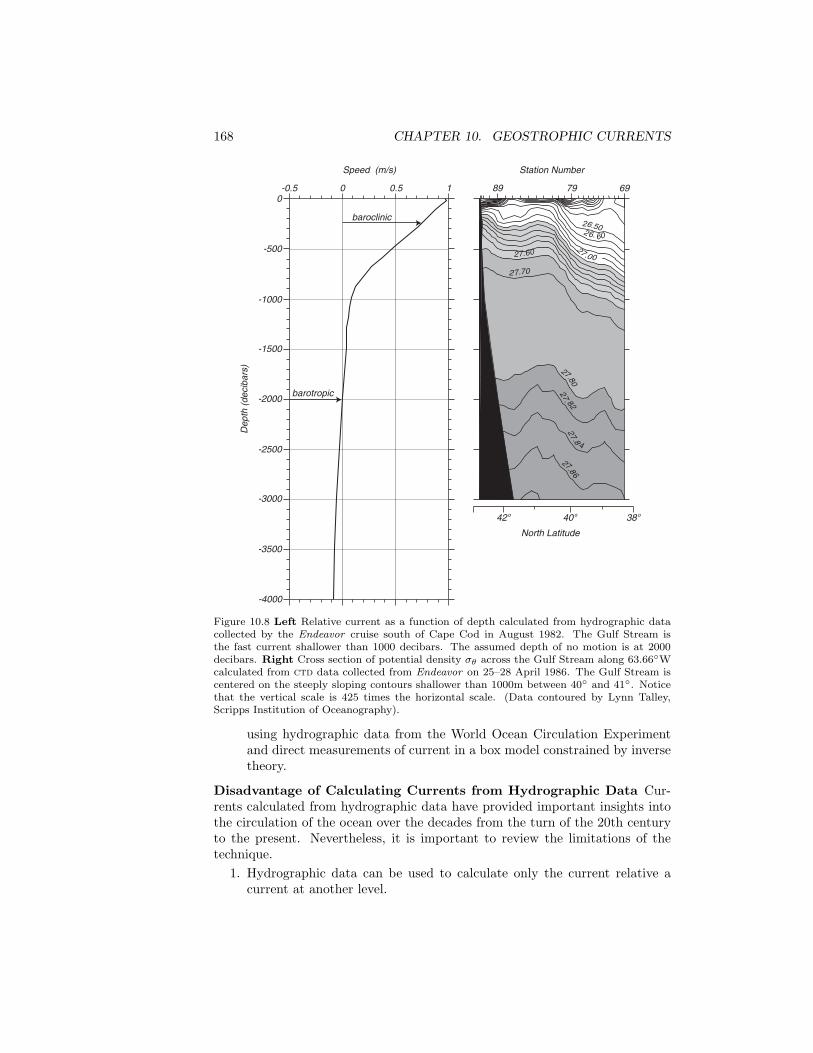
168 CHAPTER 10. GEOSTROPHIC CURRENTS
26.5026. 60
27.0027.60
2 7.70
27.8027. 82
27.8
4
27.86
79 6989
42o 40o 38o
North Latitude
Station Number
baroclinic
barotropic
-4000
-3500
-3000
-2500
-2000
-1500
-1000
-500
0-0.5 0 0.5 1
Dep
th (
deci
bars
)
Speed (m/s)
Figure 10.8 Left Relative current as a function of depth calculated from hydrographic datacollected by the Endeavor cruise south of Cape Cod in August 1982. The Gulf Stream isthe fast current shallower than 1000 decibars. The assumed depth of no motion is at 2000decibars. Right Cross section of potential density σθ across the Gulf Stream along 63.66Wcalculated from ctd data collected from Endeavor on 25–28 April 1986. The Gulf Stream iscentered on the steeply sloping contours shallower than 1000m between 40 and 41. Noticethat the vertical scale is 425 times the horizontal scale. (Data contoured by Lynn Talley,Scripps Institution of Oceanography).
using hydrographic data from the World Ocean Circulation Experimentand direct measurements of current in a box model constrained by inversetheory.
Disadvantage of Calculating Currents from Hydrographic Data Cur-rents calculated from hydrographic data have provided important insights intothe circulation of the ocean over the decades from the turn of the 20th centuryto the present. Nevertheless, it is important to review the limitations of thetechnique.
1. Hydrographic data can be used to calculate only the current relative acurrent at another level.

10.6. COMMENTS ON GEOSTROPHIC CURRENTS 169
110
110
130
150
180190
170
170
150
150
130
180
200
190
200190
210220
170
170
9070500o 0o
20o 20o
40o 40o
60o 60o
80o 80o
-20o -20o
-40o -40o
-60o -60o
-80o -80o
Figure 10.9. Mean geopotential anomaly relative to the 1,000 dbar surface in the Pacificbased on 36,356 observations. Height of the anomaly is in geopotential centimeters. If thevelocity at 1,000 dbar were zero, the map would be the surface topography of the Pacific.After Wyrtki (1979).
2. The assumption of a level of no motion may be suitable in the deep ocean,but it is usually not a useful assumption when the water is shallow suchas over the continental shelf.
3. Geostrophic currents cannot be calculated from hydrographic stations thatare close together. Stations must be tens of kilometers apart.
Limitations of the Geostrophic Equations We began this section by show-ing that the geostrophic balance applies with good accuracy to flows that exceeda few tens of kilometers in extent and with periods greater than a few days. Thebalance cannot, however, be perfect. If it were, the flow in the ocean would neverchange because the balance ignores any acceleration of the flow. The importantlimitations of the geostrophic assumption are:
1. Geostrophic currents cannot evolve with time.

170 CHAPTER 10. GEOSTROPHIC CURRENTS
-6.99
MOORING 6(206-207)recovery
18 XI 12001-day2-day3-day5-day *7-day
rel 2000best fit
Northward Speed (cm/s)
Dep
th (
m)
-6000
-5500
-5000
-4500
-4000
-3500
-3000
-2500
-2000
-15 -10 -5 0 5
Figure 10.10 Current meter measurements can be used with ctd measurements to determinecurrent as a function of depth avoiding the need for assuming a depth of no motion. Solidline: profile assuming a depth of no motion at 2000 decibars. Dashed line: profile adjustedto agree with currents measured by current meters 1–7 days before the ctd measurements.(Plots from Tom Whitworth, Texas A&M University)
2. The balance ignores acceleration of the flow, therefore it does not applyto oceanic flows with horizontal dimensions less than roughly 50 km andtimes less than a few days.
3. The geostrophic balance does not apply near the equator where the Cori-olis force goes to zero because sin ϕ → 0.
4. The geostrophic balance ignores the influence of friction.
Despite these problems, currents in the ocean are almost always very close tobeing in geostrophic balance even within a few degrees of the Equator. Strub etal. (1997) showed that currents calculated from satellite altimeter measurementsof sea-surface slope have an accuracy of ± 3–5 cm/s. Uchida, Imawaki, and Hu(1998) compared currents measured by drifters in the Kuroshio with currentscalculated from satellite altimeter measurements of sea-surface slope assuminggeostrophic balance. Using slopes over distances of 12.5 km, they found thedifference between the two measurements was ± 16 cm/s for currents up to 150cm/s, or about 10%. Johns, Watts, and Rossby (1989) measured the velocity ofthe Gulf Stream northeast of Cape Hatteras and compared the measurementswith velocity calculated from hydrographic data assuming geostrophic balance.They found that the measured velocity in the core of the stream, at depthsless than 500 m, was 10–25 cm/s faster than the velocity calculated from thegeostrophic equations using measured velocities at a depth of 2000 m. Themaximum velocity in the core was greater than 150 cm/s, so the error was≈ 10%. When they added the influence of the curvature of the Gulf Stream,

10.7. CURRENTS FROM HYDROGRAPHIC SECTIONS 171
NorthernHemisphere
p1
p2
p3
p4
v1v2
ρ1
ρ2
Level
Surface
Interface
β2 β1
γ
Figure 10.11 Slopes β of the sea surface and the slope γ of the interface between twohomogeneous, moving layers, with density ρ1 and ρ2 in the northern hemisphere. AfterNeumann and Pierson (1966: 166)
which adds an acceleration term to the geostrophic equations, the difference inthe calculated and observed velocity dropped to less than 5–10 cm/s (≈ 5%).
10.7 Currents From Hydrographic SectionsLines of hydrographic data along ship tracks are often used to produce contourplots of density in a vertical section along the track. Cross-sections of currentssometimes show sharply dipping density surfaces with a large contrast in densityon either side of the current. The baroclinic currents in the section can beestimated using a technique first proposed by Margules (1906) and describedby Defant (1961: 453). The technique allows oceanographers to estimate thespeed and direction of currents perpendicular to the section by a quick look atthe section.
To derive Margules’ equation, consider the slope ∂z/∂y of a stationaryboundary between two water masses with densities ρ1 and ρ2 (see figure 10.11).To calculate the change in velocity across the interface we assume homogeneouslayers of density ρ1 < ρ2 both of which are in geostrophic equilibrium. Althoughthe ocean does not have an idealized interface that we assumed, and the watermasses do not have uniform density, and the interface between the water massesis not sharp, the concept is still useful in practice.
The change in pressure on the interface is:
δp =∂p
∂xδx +
∂p
∂zδz, (10.18)
and the vertical and horizontal pressure gradients are obtained from (10.6):
∂p
∂z= −ρ1g + ρ1fv1 (10.19)
Therefore:
δp1 = −ρ1fv1 δx + ρ1g δz (10.20a)δp2 = −ρ2fv2 δx + ρ2g δz (10.20b)

172 CHAPTER 10. GEOSTROPHIC CURRENTS
The boundary conditions require δp1 = δp2 on the boundary if the boundary isnot moving. Equating (10.20a) with (10.20b), dividing by δx, and solving forδz/δx gives:
δz
δx≡ tan γ =
f
g
(ρ2 v2 − ρ1 v1
ρ2 − ρ1
)Because ρ1 ≈ ρ2
tan γ ≈ f
g
(ρ1
ρ1 − ρ2
)(v2 − v1) (10.21a)
tanβ1 = −f
gv1 (10.21b)
tanβ2 = −f
gv2 (10.21c)
where β is the slope of the sea surface, and γ is the slope of the boundarybetween the two water masses. Because the internal differences in density aresmall, the slope is approximately 1000 times larger than the slope of the constantpressure surfaces.
Consider the application of the technique to the Gulf Stream (figure 10.8).From the figure: ϕ = 36, ρ1 = 1026.7 kg/m3, and ρ2 = 1027.5 kg/m3 at adepth of 500 decibars. If we use the σt = 27.1 surface to estimate the slopebetween the two water masses, we see that the surface changes from a depthof 350 m to a depth of 650 m over a distance of 70 km. Therefore, tan γ =4300 × 10−6 = 0.0043, and ∆v = v2 − v1 = −0.38 m/s. Assuming v2 = 0, thenv1 = 0.38 m/s. This rough estimate of the velocity of the Gulf Stream compareswell with velocity at a depth of 500m calculated from hydrographic data (table10.4) assuming a level of no motion at 2,000 decibars.
The slope of the constant-density surfaces are clearly seen in figure 10.8.And plots of constant-density surfaces can be used to quickly estimate currentdirections and a rough value for the speed. In contrast, the slope of the seasurface is 8.4 × 10⁻⁶ or 0.84 m in 100 km if we use data from table 10.4.
Note that constant-density surfaces in the Gulf Stream slope downward tothe east, and that sea-surface topography slopes upward to the east. Constantpressure and constant density surfaces have opposite slope.
If the sharp interface between two water masses reaches the surface, it is anoceanic front, which has properties that are very similar to atmospheric fronts.
Eddies in the vicinity of the Gulf Stream can have warm or cold cores (fig-ure 10.12). Application of Margules’ method to these mesoscale eddies givesthe direction of the flow. Anticyclonic eddies (clockwise rotation in the north-ern hemisphere) have warm cores (ρ1 is deeper in the center of the eddy thanelsewhere) and the constant-pressure surfaces bow upward. In particular, thesea surface is higher at the center of the ring. Cyclonic eddies are the reverse.
10.8 Lagrangean Measurements of CurrentsOceanography and fluid mechanics distinguish between two techniques for mea-suring currents: Lagrangean and Eulerian. Lagrangean techniques follow a

10.8. LAGRANGEAN MEASUREMENTS OF CURRENTS 173
ρ1
p0
ρ2
ρ2
p4
p3
p2
p5
p1
p0
p1
p2
p3
p4
p5
ρ1
Warm-core ring Cold-core ring
Figure 10.12 Shape of constant-pressure surfaces pi and the interface between two watermasses of density ρ1, ρ2 if the upper is rotating faster than the lower. Left: Anticyclonicmotion, warm-core eddy. Right: Cyclonic, cold-core eddy. Note that the sea surface p0
slopes up toward the center of the warm-core ring, and the constant-density surfaces slopedown toward the center. Circle with dot is current toward the reader, circle with cross iscurrent away from the reader. After Defant (1961: 466).
water particle. Eulerian techniques measure the velocity of water at a fixedposition.
Basic Technique Lagrangean techniques track the position of a drifter thatfollows a water parcel either on the surface or deeper within the water column.The mean velocity over some period is calculated from the distance betweenpositions at the beginning and end of the period divided by the period. Errorsare due to:
1. Errors in determining the position of the drifter.
2. The failure of the drifter to follow a parcel of water. We assume thedrifter stays in a parcel of water, but external forces acting on the driftercan cause it to drift relative to the water.
3. Sampling errors. Drifters go only where drifters want to go. And drifterswant to go to convergent zones. Hence drifters tend to avoid areas ofdivergent flow.
Satellite Tracked Surface Drifters Surface drifters consist of a drogue plusa float that is usually tracked by the Argos system on meteorological satellites(Swenson and Shaw, 1990). The buoy carries a simple radio transmitter witha very stable frequency F0. A receiver on the satellite receives the signal anddetermines the Doppler shift F as a function of time t (figure 10.13). TheDoppler frequency is
F =dR
dt
F0
c+ F0
where R is the distance to the buoy, c is the velocity of light. The closer thebuoy to the satellite the more rapidly the frequency changes. When F = F0 therange is a minimum. This is the time of closest approach, and the satellite’svelocity vector is perpendicular to the line from the satellite to the buoy. Thetime of closest approach and the time rate of change of Doppler frequency atthat time gives the buoy’s position relative to the orbit with a 180ambiguity.

174 CHAPTER 10. GEOSTROPHIC CURRENTS
F0F
t
B
B
E
A2
A1
K
Figure 10.13 Satellite systems, especially System Argos, use radio signals transmitted fromsurface buoys to determine the position of the buoy. The satellite S receives a radio signalfrom the buoy B. The time rate of change of the signal, the Doppler shift F , is a functionof buoy position and distance from the satellite’s track. The recorded Doppler signal istransmitted to ground stations E, which relays the information to processing centers A viacontrol stations K. After Dietrich et al. (1980: 149).
Because the orbit is accurately known, and because the buoy can be observedmany times, its position can be determined without ambiguity.
The accuracy of the position depends on the stability of the frequency trans-mitted by the buoy. The Argos system tracks buoys with an accuracy of ±1–2km, collecting 1–8 positions per day depending on latitude. Because 1 cm/s ≈1 km/day, and because typical values of currents in the ocean range from oneto two hundred centimeters per second, this is an very useful accuracy.
Holey-Sock Drifters Many types of surface drifters have been developed, cul-minating with the holey-sock drifter now widely used to track surface currents.The drifter consists of a circular, cylindrical drogue of cloth 1 m in diameter by15 m long with 14 large holes cut in the sides. The weight of the drogue is sup-ported by a submerged float set 3 m below the surface. The submerged float istethered to a partially submerged surface float carrying the Argos transmitter.
Niiler et al. (1995) carefully measured the rate at which wind blowing onthe surface float pulls the drogue through the water, and they found that thebuoy moves 12 ± 9 to the right of the wind at a speed
Us = (4.32 ± 0.67×) 10−2 U10
DAR+ (11.04 ± 1.63)
D
DAR(10.22)
where DAR is the drag area ratio defined as the drogue’s drag area divided by

10.8. LAGRANGEAN MEASUREMENTS OF CURRENTS 175
the sum of the tether’s drag area and the surface float’s drag area, and D is thedifference in velocity of the water between the top of the cylindrical drogue andthe bottom. If DAR > 40, then the drift Us < 1 cm/s for U10 < 10 m/s.
Subsurface Drifters (Swallow and Richardson Floats) Subsurface drift-ers are widely used for measuring currents below the mixed layer. Subsurfacedrifters are neutrally buoyant chambers tracked by sonar using the sofar—Sound Fixing and Ranging—system for listening to sounds in the sound channel.The chamber can be a section of aluminum tubing containing electronics andcarefully weighed to have the same density as water at a predetermined depth.Aluminum is chosen because it has a compressibility less than water.
The drifter has errors due to the failure of the drifter to stay within the samewater mass. Often the errors are sufficiently small that the only important erroris due to tracking accuracy.
The primary disadvantage of the neutrally buoyant drifter is that trackingsystems are not available throughout the ocean.
Pop-Up Drifters (ALACE, PALACE, and ARGO Drifters) : Autono-mous Lagrangean Circulation Explorer (alace) drifters (figure 10.14) are de-signed to cycle between the surface and some predetermined depth. The drifterspends roughly 10 days at depth, and periodically returns to the surface to re-
From InternalReservoir
17cm
107 cm
Evacuation Port
Camping Disk
Internal Reservoir
Argos Transmitter
Controller andCircuit Boards
MicroprocessorBattery Packs
Pump Battery PacksMotorFilter
Hydraulic PumpLatching Valve
Pressure Case
Argos Antenna Port
External Bladder
One-WayCheck Valve
70 cm
Wobble Plate
Self-PrimingChannel
Piston
To InternalReservoir
Inlet Channel
Motor
Latching Valve
Descending State
Ascending StateArgos
Antenna
Figure 10.14 The Autonomous Lagrangean Circulation Explorer (ALACE) drifters are widelyused by the World Ocean Circulation Experiment to measure mid-depth currents. Left:Schematic of the drifter. To ascend, the hydraulic pump moves oil from an internal reservoirto an external bladder, reducing the drifter’s density. To descend, the latching valve is openedto allow oil to flow back into the internal reservoir. The antenna is mounted to the end cap.Right: Expanded schematic of the hydraulic system. The motor rotates the wobble plateactuating the piston which pumps hydraulic oil. After Davis et al. (1992).

176 CHAPTER 10. GEOSTROPHIC CURRENTS
port it’s position and other information using the Argos system (Davis et al.,1992). The drifter thus combines the best aspects of surface and neutrally-buoyant drifters. It is able to track deep currents, it is autonomous of acoustictracking systems, and it can be tracked anywhere in the ocean by satellite. Themaximum depth is near 2 km, and the drifter carries sufficient power to complete70 to 1,000 m or 50 cycles to 2,000 m.
palace drifters are profiling alace drifters. They measure the profile oftemperature and salinity between the drifting depth and the surface when thedrifter pops up to the surface. argo drifters are the latest version of the drifter.Thousands of argo drifters will be launched for the Global Ocean Data Assim-ilation Experiment godae.
Lagrangean Measurements Using Tracers Perhaps the best way for fol-lowing water parcels is to tag the parcel with molecules not normally found inthe ocean. Thanks to atomic bomb tests in the 1950s and the recent exponen-tial increase of chlorofluorocarbons in the atmosphere, such tracers have beenintroduced into the ocean in large quantities. See §13.3 for a list of tracers usedin oceanography. The distribution of trace molecules is used to infer the move-ment of the water. The technique is especially useful for calculating velocity ofdeep water masses averaged over decades and for calculating eddy diffusivities.
The distribution of trace molecules is calculated from the concentration ofthe molecules in water samples collected on hydrographic sections and surveys.Because the collection of data is expensive and slow, there are few repeatedsections. Figure 10.15 shows two maps of the distribution of tritium in theNorth Atlantic collected in 1972–1973 by the Geosecs Program and in 1981, adecade later. The sections show that tritium, introduced into the atmosphereduring the atomic bomb tests in the atmosphere in the 1950s to 1972, penetratedto depths below 4 km only north of 40N by 1971 and to 35N by 1981. Thisshows that deep currents are very slow, about 1.6 mm/s in this example.
Because the deep currents are so small, we can question what process areresponsible for the observed distribution of tracers. Both turbulent diffusionand advection by currents can fit the observations. Hence, does figure 10.15give mean currents in the deep Atlantic, or the turbulent diffusion of tritium?
Another useful tracer is the temperature and salinity of the water. Wewill consider these observations in §13.3 where we describe the core methodfor studying deep circulation. Here, we note that avhrr observations of surfacetemperature of the ocean are an additional source of information about currents.
Sequential infrared images of surface temperature are used to calculate thedisplacement of features in the images (figure 10.16). The technique is especiallyuseful for surveying the variability of currents near shore. Land provides ref-erence points from which displacement can be calculated accurately, and largetemperature contrasts can be found in many regions in some seasons.
There are two important limitations.1. Many regions have extensive cloud cover, and the ocean cannot be seen.2. Flow is primarily parallel to temperature fronts, and strong currents can
exist along fronts even though the front may not move. It is therefore

10.8. LAGRANGEAN MEASUREMENTS OF CURRENTS 177
0.6
5
0.8
0.2
0.6
0.4
0.6
0.8
0.8
0.8
0.8
0.8
3
2
1
2
1
1
2
2
34
5 65
H
H
L
L
42
2
4
1
0.2
L
0.2 0.4
0.8
2
2
22
444 5
1
H 33 3
3
3
Western North Atlantic (1981)
Western North Atlantic (1972)
80o70o60o50o40o30o20o10o0o10o
0
-6000
-5000
-4000
-3000
-2000
-1000
Dep
th (
m)
80o70o60o50o40o30o20o10o0o10o
0
-6000
-5000
-4000
-3000
-2000
-1000
Dep
th (
m)
Figure 10.15 Distribution of tritium along a section through the western basins in the NorthAtlantic, measured in 1972 (Top) and remeasured in 1981 (Bottom). Units are tritiumunits, where one tritium unit is 1018 (tritium atoms)/(hydrogen atoms) corrected to theactivity levels that would have been observed on 1 January 1981. Compare this figure to thedensity in the ocean shown in figure 13.10. After Toggweiler (1994).
essential to track the motion of small eddies embedded in the flow nearthe front and not the position of the front.
The Rubber Duckie Spill On January 10, 1992 a 12.2-m container with29,000 bathtub toys (including rubber ducks) washed overboard from a con-tainer ship at 44.7N, 178.1E. Ten months later the toys began washing ashorenear Sitka, Alaska. A similar accident on May 27, 1990 released 80,000 Nike-brand shoes at 48N, 161W when waves washed containers from the Hansa

178 CHAPTER 10. GEOSTROPHIC CURRENTS
Figure 10.16 Ocean temperature and current patterns are combined in this avhrr analysis.Surface currents were computed by tracking the displacement of small thermal or sedimentfeatures between a pair of images. A directional edge-enhancement filter was applied here todefine better the different water masses. Warm water is shaded darker. From Ocean Imaging,Solana Beach, California, with permission.
Carrier(figure 10.17). The spill and the eventual recovery of the toys provedto be a good test of a numerical model for calculating the trajectories of oilspills developed by Ebbesmeyer and Ingraham (1992, 1994). They calculatedthe possible trajectories of the spilled rubber ducks using the Ocean SurfaceCurrent Simulations oscurs numerical model driven by winds calculated fromthe Fleet Numerical Oceanography Center’s daily sea-level pressure data. Thecalculated trajectories agreed well with observed locations of drifters found onthe shore. Using a 50% increase in windage coefficient and a 5 decrease in the

10.9. EULERIAN MEASUREMENTS 179
170o -170o -150o -130o -110o
60o
50o
40o
30o
20o
North America
10o
Hawaii
Bering Sea
1992-94
1990-92
1961-63
1984-86
1959-64
North Pacific Ocean
Origin of
Toy Spill
Figure 10.17 Trajectories that spilled rubber duckies would have followed had they beenspilled on January 10 of different years. Five trajectories were selected from a set of 48simulations of the spill each year between 1946 and 1993. The trajectories begin on January10 and end two years later (solid symbols). Grey symbols indicate positions on November16 of the year of the spill. Hence the grey circle gives the location where rubber ducks firstcame ashore near Sitka. The code at lower left gives the dates of the trajectories. AfterEbbesmeyer and Ingraham (1994).
angle of deflection function, the toys arrived near Sitka, Alaska at the time ofthe first recoveries on November 16, 1992.
10.9 Eulerian MeasurementsEulerian measurements have been made by many different types of current me-ters attached to many types of moorings or ships.
Moorings are deployed by ships, and they may last for months to longer thana year (figure 10.18). Because the mooring must be deployed and recovered bydeep-sea research ships, the technique is expensive. Submerged moorings arepreferred for several reasons: the surface float is not forced by high frequency,strong, surface currents; the mooring is out of sight and it does not attract theattention of fishermen; and the floatation is usually deep enough to avoid beingcaught by fishing nets. Errors are due to:
1. Mooring motion. Subsurface moorings move least. Surface moorings instrong currents move most, and are seldom used.
2. Inadequate Sampling. Moorings tend not to last long enough to give ac-curate estimates of mean velocity or interannual variability of the velocity.
3. Fouling of the sensors by marine organisms, especially instruments de-ployed for more than a few weeks close to the surface.
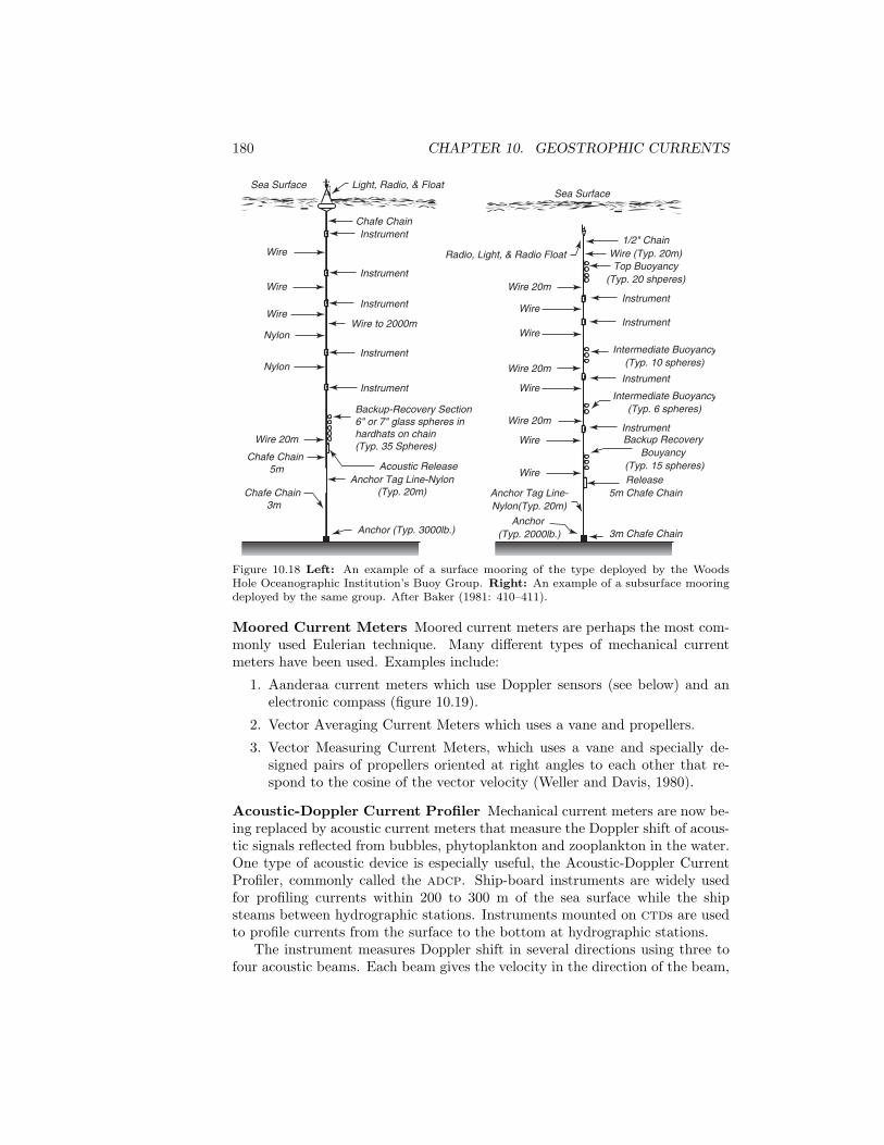
180 CHAPTER 10. GEOSTROPHIC CURRENTS
Wire 20m
Chafe Chain 5m
Chafe Chain 3m
Nylon
Nylon
Wire
Wire
Wire
Sea Surface
Chafe ChainInstrument
Instrument
Instrument
Instrument
Instrument
Wire to 2000m
Backup-Recovery Section 6" or 7" glass spheres inhardhats on chain(Typ. 35 Spheres)
Acoustic ReleaseAnchor Tag Line-Nylon
(Typ. 20m)
Anchor (Typ. 3000lb.)
Light, Radio, & Float
Wire 20m
Wire
Wire
Wire 20m
Wire
Wire 20m
Wire
Sea Surface
Wire
Anchor Tag Line-Nylon(Typ. 20m)
Instrument
Instrument
Instrument
Instrument
1/2" ChainWire (Typ. 20m)Radio, Light, & Radio FloatTop Buoyancy
(Typ. 20 shperes)
Intermediate Buoyancy(Typ. 10 spheres)
Intermediate Buoyancy(Typ. 6 spheres)
Backup Recovery Bouyancy
(Typ. 15 spheres)
3m Chafe Chain
Release 5m Chafe Chain
Anchor (Typ. 2000lb.)
Figure 10.18 Left: An example of a surface mooring of the type deployed by the WoodsHole Oceanographic Institution’s Buoy Group. Right: An example of a subsurface mooringdeployed by the same group. After Baker (1981: 410–411).
Moored Current Meters Moored current meters are perhaps the most com-monly used Eulerian technique. Many different types of mechanical currentmeters have been used. Examples include:
1. Aanderaa current meters which use Doppler sensors (see below) and anelectronic compass (figure 10.19).
2. Vector Averaging Current Meters which uses a vane and propellers.
3. Vector Measuring Current Meters, which uses a vane and specially de-signed pairs of propellers oriented at right angles to each other that re-spond to the cosine of the vector velocity (Weller and Davis, 1980).
Acoustic-Doppler Current Profiler Mechanical current meters are now be-ing replaced by acoustic current meters that measure the Doppler shift of acous-tic signals reflected from bubbles, phytoplankton and zooplankton in the water.One type of acoustic device is especially useful, the Acoustic-Doppler CurrentProfiler, commonly called the adcp. Ship-board instruments are widely usedfor profiling currents within 200 to 300 m of the sea surface while the shipsteams between hydrographic stations. Instruments mounted on ctds are usedto profile currents from the surface to the bottom at hydrographic stations.
The instrument measures Doppler shift in several directions using three tofour acoustic beams. Each beam gives the velocity in the direction of the beam,

10.10. IMPORTANT CONCEPTS 181
Mooring Line
RCM AcousticDoppler Current Sensor
Optional Sensors: -Oxygen -Pressure -Temperature -Turbidity
Electronics andData Storage
Mooring Line
Figure 10.19 An example of a moored current meter, the rcm 9 produced by AanderaaInstruments. Two components of horizontal velocity are measured by an acoustic currentmeter, and the directions are referenced to north using an internal Hall-effect compass. Theelectronics, data recorder, and battery are in the pressure-resistant housing. Accuracy is±0.15 cm/s and ±5. (Courtesy Aanderaa Instruments)
and the combination of several beams gives two or three components of thevelocity.
Acoustic Tomography Another acoustic technique uses acoustic signals trans-mitted through the sound channel to and from a few moorings spread out acrossoceanic regions. The technique is expensive because it requires many deep moor-ings and loud sound sources. It promises, however, to obtain information dif-ficult to obtain by other means. The number of acoustic paths across a regionrises as the square of the number of moorings. And, the signal propagatingalong the sound channel has many modes, some that stay near the axis of thechannel, others that propagate close to the sea surface and bottom (See figure3.16). The various modes give the vertical temperature structure in the ocean,and the many paths in the horizontal give the spatial distribution of tempera-ture. If one mooring retransmits the signal it receives from another mooring, thetime for the signal to propagate in one direction minus the time for the signalto propagate in the reverse direction, the reciprocal travel time, is proportionalto current component parallel to the acoustic path.
10.10 Important Concepts1. Pressure distribution is almost precisely the hydrostatic pressure obtained
by assuming the ocean is at rest. Pressure is therefore calculated veryaccurately from measurements of temperature and conductivity as a func-

182 CHAPTER 10. GEOSTROPHIC CURRENTS
tion of pressure using the equation of state of seawater. Hydrographicdata give the relative, internal pressure field of the ocean.
2. Flow in the ocean is in almost exact geostrophic balance except for flowin the upper and lower boundary layers. Coriolis force almost exactlybalances the horizontal pressure gradient.
3. Satellite altimetric observations of the oceanic topography give the surfacegeostrophic current. The calculation of topography requires an accurategeoid, which is known with sufficient accuracy only over distances exceed-ing a few thousand kilometers. If the geoid is not known, altimeters canmeasure the change in topography as a function of time, which gives thechange in surface geostrophic currents.
4. Topex/Poseidon and Jason are the most accurate altimeter systems, andthey can measure the topography or changes in topography with an accu-racy of ±4 cm.
5. Hydrographic data are used to calculate the internal geostrophic currentsin the ocean relative to known currents at some level. The level can besurface currents measured by altimetry or an assumed level of no motionat depths below 1–2 km.
6. Flow in the ocean that is independent of depth is called barotropic flow,flow that depends on depth is called baroclinic flow. Hydrographic datagive only the baroclinic flow.
7. Geostrophic flow cannot change with time, so the flow in the ocean is notexactly geostrophic. The geostrophic method does not apply to flows atthe equator where the Coriolis force vanishes.
8. Slopes of constant density or temperature surfaces seen in a cross-sectionof the ocean can be used to estimate the speed of flow through the section.
9. Lagrangean techniques measure the position of a parcel of water in theocean. The position can be determined using surface or subsurface drifters,or chemical tracers such as tritium.
10. Eulerian techniques measure the velocity of flow past a point in the ocean.The velocity of the flow can be measured using moored current meters oracoustic velocity profilers on ships, ctds or moorings.

Chapter 11
Wind Driven OceanCirculation
What drives the ocean currents? At first, we might answer, the winds drivethe circulation. But if we think more carefully about the question, we mightnot be so sure. We might notice, for example, that strong currents, such as theNorth Equatorial Countercurrents in the Atlantic and Pacific Oceans go upwind.Spanish navigators in the 16th century noticed strong northward currents alongthe Florida coast that seemed to be unrelated to the wind. How can this happen?And, why are strong currents found offshore of east coasts but not offshore ofwest coasts?
Answers to the questions can be found in a series of three remarkable paperspublished from 1947 to 1951. In the first, Harald Sverdrup (1947) showed thatthe circulation in the upper kilometer or so of the ocean is directly related tothe curl of the wind stress. Henry Stommel (1948) showed that the circulationin oceanic gyres is asymmetric because the Coriolis force varies with latitude.Finally, Walter Munk (1950) added eddy viscosity and calculated the circulationof the upper layers of the Pacific. Together the three oceanographers laid thefoundations for a modern theory of ocean circulation.
11.1 Sverdrup’s Theory of the Oceanic CirculationWhile Sverdrup was analyzing observations of equatorial currents, he came upon(11.7) below relating the curl of the wind stress to mass transport within theupper ocean. In deriving the relationship, Sverdrup assumed that the flow isstationary, that lateral friction and molecular viscosity are small, and that tur-bulence near the sea surface can be described using a vertical eddy viscosity.He also assumed that the flow is baroclinic and that the wind-driven circula-tion vanishes at some depth of no motion. From (8.9 and 8.12) the horizontalcomponents of the momentum equation are:
∂p
∂x= f ρ v +
∂
∂z
(Az
∂u
∂z
)(11.1a)
183

184 CHAPTER 11. WIND DRIVEN OCEAN CIRCULATION
∂p
∂y= −f ρ u +
∂
∂z
(Az
∂v
∂z
)(11.1b)
Sverdrup integrated these equations from the surface to a depth −D equalto or greater than the depth at which the horizontal pressure gradient becomeszero. He defined:
∂P
∂x=
0∫−D
∂p
∂xdz,
∂P
∂y=
0∫−D
∂p
∂ydz, (11.2a)
Mx ≡0∫
−D
ρ u(z) dz, My ≡0∫
−D
ρ v(z) dz, (11.2b)
where Mx, My are the mass transports in the wind-driven layer extending downto an assumed depth of no motion.
The horizontal boundary condition at the sea surface is the wind stress, andthe boundary at depth −D is zero stress because the currents go to zero:(
Az∂u
∂z
)0
= Tx
(Az
∂u
∂z
)−D
= 0(Az
∂v
∂z
)0
= Ty
(Az
∂v
∂z
)−D
= 0 (11.3)
where Tx and Ty are the components of the wind stress.Using these definitions and boundary conditions, (11.1) become:
∂P
∂x= f My + Tx (11.4a)
∂P
∂y= −f Mx + Ty (11.4b)
In a similar way, Sverdrup integrated the continuity equation (7.19) over thesame vertical depth, assuming the vertical velocity at the surface and at depth−D are zero, to obtain:
∂Mx
∂x+
∂My
∂y= 0 (11.5)
Differentiating (11.4a) with respect to y and (11.4b) with respect to x, sub-tracting, and using (11.5) gives:
β My =∂Ty
∂x− ∂Tx
∂y
β My = curlz(T ) (11.6)
where β ≡ ∂f/∂y is the rate of change of Coriolis parameter with latitude, andwhere curlz(T ) is the vertical component of the curl of the wind stress.

11.1. SVERDRUP’S THEORY OF THE OCEANIC CIRCULATION 185
Streamlines of MassTransport
Boundaries of CounterCurrent
Values of stream function, Ψ, given in units of 10 metric tons/sec
25 20 15 10 5
0
0
0
0
-10 -5
105
5100
15
-15
15
-15
-5
-5
-10
-10
-20
-160o -150o -140o -130o -120o -110o -100o -90o -80o
-10o
0o
10o
20o
30o
Figure 11.1 Streamlines of mass transport in the eastern Pacific calculatedfrom Sverdrup’s theory using mean annual wind stress. After Reid (1948).
This is an important and fundamental result—the northward mass transportof wind driven currents is equal to the curl of the wind stress. Note that Sverdrupallowed f to vary with latitude. We will see later that this is essential.
We calculate β from
β ≡ ∂f
∂y=
2 Ω cos ϕ
R(11.7)
where R is Earth’s radius and ϕ is latitude.Over much of the open ocean, especially in the tropics, the wind is zonal
and ∂Ty/∂x is sufficiently small that
My ≈ − 1β
∂Tx
∂y(11.8)
Substituting (11.8) into (11.5), Sverdrup obtained:
∂Mx
∂x= − 1
2 Ω cos ϕ
(∂Tx
∂ytanϕ +
∂2Tx
∂y2R
)(11.9)
Sverdrup integrated this equation from a north-south eastern boundary atx = 0, assuming no flow into the boundary. This requires Mx = 0 at x = 0.Then
Mx = − ∆x
2 Ω cos ϕ
[⟨∂Tx
∂y
⟩tanϕ +
⟨∂2Tx
∂y2
⟩R
](11.10)
where ∆x is the distance from the eastern boundary of the ocean basin, andbrackets indicate zonal averages of the wind stress (figure 11.1).

186 CHAPTER 11. WIND DRIVEN OCEAN CIRCULATION
-7 -5 -3 -1 1 3 5
-10
-5
5
10
15
20
25
Latitude
My
10 30 50 70-10-30-50
Latitude
Mx
North EquatorialCurrent
Westward EastwardSouthward Northward
-10
-5
5
10
15
20
25
North EquatorialCounter Current
South EquatorialCurrent
Figure 11.2 Mass transport in the eastern Pacific calculated from Sverdrup’s theory usingobserved winds with 11.8 and 11.10 (solid lines) and pressure calculated from hydrographicdata from ships with 11.4 (dots). Transport is in tons per second through a section one meterwide extending from the sea surface to a depth of one kilometer. Note the difference in scalebetween My and Mx. After Reid (1948).
To test his theory, Sverdrup compared transports calculated from knownwinds in the eastern tropical Pacific with transports calculated from hydro-graphic data collected by the Carnegie and Bushnell in October and November1928, 1929, and 1939 between 34N and 10S and between 80W and 160W.The hydrographic data were used to compute P by integrating from a depthof D = −1000 m. The comparison, figures 11.2, showed not only that thetransports can be accurately calculated from the wind, but also that the theorypredicts wind-driven currents going upwind.
Comments on Sverdrup’s Solutions1. Sverdrup assumed i) The internal flow in the ocean is geostrophic; ii) there
is a uniform depth of no motion; and iii) Ekman’s transport is correct. Weexamined Ekman’s theory in Chapter 9, and the geostrophic balance inChapter 10. We know little about the depth of no motion in the tropicalPacific.
2. The solutions are limited to the east side of the oceans because Mx growswith x. The result comes from neglecting friction which would eventuallybalance the wind-driven flow. Nevertheless, Sverdrup solutions have beenused for describing the global system of surface currents. The solutionsare applied throughout each basin all the way to the western limit of thebasin. There, conservation of mass is forced by including north-southcurrents confined to a thin, horizontal boundary layer (figure 11.3).
3. Only one boundary condition can be satisfied, no flow through the easternboundary. More complete descriptions of the flow require more completeequations.

11.1. SVERDRUP’S THEORY OF THE OCEANIC CIRCULATION 187
0
0
20
0
00
20
0
20
0
30
20
20
100
60
20
40
40o
20o
0o
-20o
-40o
30o 60o 90o 120o 150o 180o -150o -120o -90o -60o -30o 0o
Figure 11.3 Depth-integrated Sverdrup transport applied globally using the wind stress fromHellerman and Rosenstein (1983). Contour interval is 10 Sverdrups. After Tomczak andGodfrey (1994: 46).
4. The solutions do not give the vertical distribution of the current.
5. Results were based on data from two cruises plus average wind data as-suming a steady state. Later calculations by Leetmaa, McCreary, andMoore (1981) using more recent wind data produces solutions with sea-sonal variability that agrees well with observations provided the level ofno motion is at 500 m. If another depth were chosen, the results are notas good.
6. Wunsch (1996: §2.2.3) after carefully examining the evidence for a Sver-drup balance in the ocean concluded we do not have sufficient informationto test the theory. He writes
The purpose of this extended discussion has not been to disapprovethe validity of Sverdrup balance. Rather, it was to emphasize the gapcommonly existing in oceanography between a plausible and attrac-tive theoretical idea and the ability to demonstrate its quantitativeapplicability to actual oceanic flow fields.—Wunsch (1996).
Wunsch, however, notes
Sverdrup’s relationship is so central to theories of the ocean circu-lation that almost all discussions assume it to be valid without anycomment at all and proceed to calculate its consequences for higher-order dynamics . . . it is difficult to overestimate the importance ofSverdrup balance.—Wunsch (1996).
But the gap is shrinking. Measurements of mean stress in the equatorialPacific (Yu and McPhaden, 1999) show that the flow there is in Sverdrupbalance.
Stream Lines, Path Lines, and the Stream Function Before discussingmore about the ocean’s wind-driven circulation, we need to introduce the con-cept of stream lines and the stream function (see Kundu, 1990: 51 & 66).

188 CHAPTER 11. WIND DRIVEN OCEAN CIRCULATION
x
x + dx
-u dy
v dx
y
x
ψ+
dψ
ψ
Figure 11.4 Volume transport between stream lines in atwo-dimensional, steady flow. After Kundu (1990: 68).
At each instant in time, we can represent a flow field by a vector velocity ateach point in space. The instantaneous curves that are everywhere tangent tothe direction of the vectors are called the stream lines of the flow. If the flow isunsteady, the pattern of stream lines change with time.
The trajectory of a fluid particle, the path followed by a Lagrangean drifter,is called the path line in fluid mechanics. The path line is the same as the streamline for steady flow, and they are different for an unsteady flow.
We can simplify the description of two-dimensional, incompressible flows byusing the stream function ψ defined by:
u ≡ ∂ψ
∂y, v ≡ −∂ψ
∂x, (11.11)
The stream function is often used because it is a scalar from which the vectorvelocity field can be calculated. This leads to simpler equations for some flows.
Stream functions are also useful for visualizing the flow. At each instant,the flow is parallel to lines of constant ψ. Thus if the flow is steady, the lines ofconstant stream function are the paths followed by water parcels.
The volume rate of flow between any two stream lines of a steady flow isdψ, and the volume rate of flow between two stream lines ψ1 and ψ2 is equalto ψ1 − ψ2. To see this, consider an arbitrary line dx = (dx, dy) between twostream lines (figure 11.4). The volume rate of flow between the stream lines is:
v dx + (−u) dy = −∂ψ
∂xdx − ∂ψ
∂ydy = −dψ (11.12)
and the volume rate of flow between the two stream lines is numerically equalto the difference in their values of ψ.
Now, lets apply the concepts to satellite-altimeter maps of the oceanic to-pography. In §10.3 we wrote (10.10)
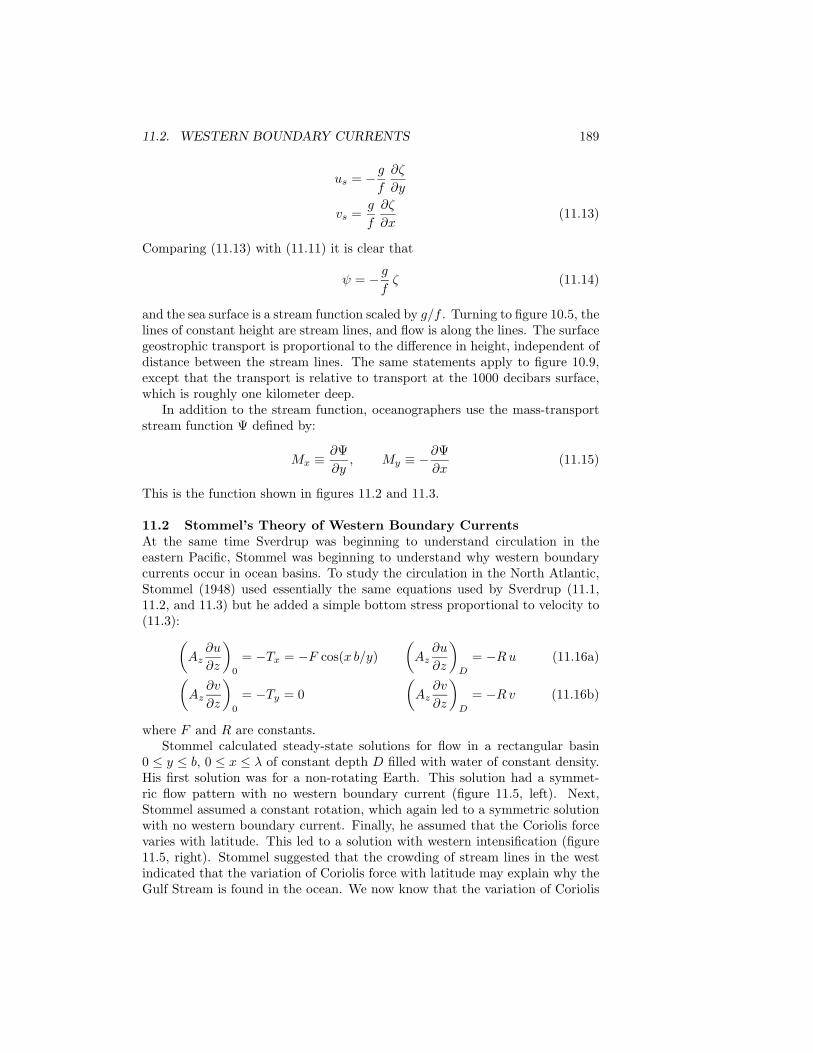
11.2. WESTERN BOUNDARY CURRENTS 189
us = − g
f
∂ζ
∂y
vs =g
f
∂ζ
∂x(11.13)
Comparing (11.13) with (11.11) it is clear that
ψ = − g
fζ (11.14)
and the sea surface is a stream function scaled by g/f . Turning to figure 10.5, thelines of constant height are stream lines, and flow is along the lines. The surfacegeostrophic transport is proportional to the difference in height, independent ofdistance between the stream lines. The same statements apply to figure 10.9,except that the transport is relative to transport at the 1000 decibars surface,which is roughly one kilometer deep.
In addition to the stream function, oceanographers use the mass-transportstream function Ψ defined by:
Mx ≡ ∂Ψ∂y
, My ≡ −∂Ψ∂x
(11.15)
This is the function shown in figures 11.2 and 11.3.
11.2 Stommel’s Theory of Western Boundary CurrentsAt the same time Sverdrup was beginning to understand circulation in theeastern Pacific, Stommel was beginning to understand why western boundarycurrents occur in ocean basins. To study the circulation in the North Atlantic,Stommel (1948) used essentially the same equations used by Sverdrup (11.1,11.2, and 11.3) but he added a simple bottom stress proportional to velocity to(11.3):(
Az∂u
∂z
)0
= −Tx = −F cos(x b/y)(
Az∂u
∂z
)D
= −R u (11.16a)(Az
∂v
∂z
)0
= −Ty = 0(
Az∂v
∂z
)D
= −R v (11.16b)
where F and R are constants.Stommel calculated steady-state solutions for flow in a rectangular basin
0 ≤ y ≤ b, 0 ≤ x ≤ λ of constant depth D filled with water of constant density.His first solution was for a non-rotating Earth. This solution had a symmet-ric flow pattern with no western boundary current (figure 11.5, left). Next,Stommel assumed a constant rotation, which again led to a symmetric solutionwith no western boundary current. Finally, he assumed that the Coriolis forcevaries with latitude. This led to a solution with western intensification (figure11.5, right). Stommel suggested that the crowding of stream lines in the westindicated that the variation of Coriolis force with latitude may explain why theGulf Stream is found in the ocean. We now know that the variation of Coriolis
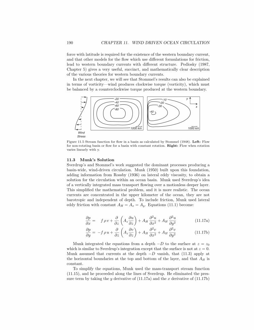
190 CHAPTER 11. WIND DRIVEN OCEAN CIRCULATION
force with latitude is required for the existence of the western boundary current,and that other models for the flow which use different formulations for friction,lead to western boundary currents with different structure. Pedlosky (1987,Chapter 5) gives a very useful, succinct, and mathematically clear descriptionof the various theories for western boundary currents.
In the next chapter, we will see that Stommel’s results can also be explainedin terms of vorticity—wind produces clockwise torque (vorticity), which mustbe balanced by a counterclockwise torque produced at the western boundary.
-80-60-40-20 -10
-20-30
-40
1000 km1000 km
WindStress
y
x
Figure 11.5 Stream function for flow in a basin as calculated by Stommel (1948). Left: Flowfor non-rotating basin or flow for a basin with constant rotation. Right: Flow when rotationvaries linearly with y.
11.3 Munk’s SolutionSverdrup’s and Stommel’s work suggested the dominant processes producing abasin-wide, wind-driven circulation. Munk (1950) built upon this foundation,adding information from Rossby (1936) on lateral eddy viscosity, to obtain asolution for the circulation within an ocean basin. Munk used Sverdrup’s ideaof a vertically integrated mass transport flowing over a motionless deeper layer.This simplified the mathematical problem, and it is more realistic. The oceancurrents are concentrated in the upper kilometer of the ocean, they are notbarotropic and independent of depth. To include friction, Munk used lateraleddy friction with constant AH = Ax = Ay. Equations (11.1) become:
∂p
∂x= f ρ v +
∂
∂z
(Az
∂u
∂z
)+ AH
∂2u
∂x2+ AH
∂2u
∂y2(11.17a)
∂p
∂y= −f ρ u +
∂
∂z
(Az
∂v
∂z
)+ AH
∂2v
∂x2+ AH
∂2v
∂y2(11.17b)
Munk integrated the equations from a depth −D to the surface at z = z0
which is similar to Sverdrup’s integration except that the surface is not at z = 0.Munk assumed that currents at the depth −D vanish, that (11.3) apply atthe horizontal boundaries at the top and bottom of the layer, and that AH isconstant.
To simplify the equations, Munk used the mass-transport stream function(11.15), and he proceeded along the lines of Sverdrup. He eliminated the pres-sure term by taking the y derivative of (11.17a) and the x derivative of (11.17b)

11.3. MUNK’S SOLUTION 191
10o
0o
20o
30o
40o
60o
50o
10o
0o
20o
30o
40o
60o
50o
-10o
10-1 1
01000 2000 3000 4000 5000 6000 7000 8000 9000 100000
1000 2000 3000 4000 5000 6000 7000 8000 9000 100000
dynes cm-2
anddynes cm-3
X
108dTx/dy
τx
ϕb
ϕa
ϕb
ϕa
ϕb
ϕb
ϕb
ϕa
ϕa
Figure 11.6 Left: Mean annual wind stress Tx(y) over the Pacific and the curl of the windstress. ϕb are the northern and southern boundaries of the gyres, where My = 0 and curlτ = 0. ϕ0 is the center of the gyre. Upper Right: The mass transport stream function fora rectangular basin calculated by Munk (1950) using observed wind stress for the Pacific.Contour interval is 10 Sverdrups. The total transport between the coast and any point x, yis ψ(x, y).The transport in the relatively narrow northern section is greatly exaggerated.Lower Right: North-South component of the mass transport. After Munk (1950).
to obtain the equation for mass transport:
AH∇4Ψ︸ ︷︷ ︸Friction
− β∂Ψ∂x
= − curlzT︸ ︷︷ ︸Sverdrup Balance
(11.18)
where
∇4 =∂4
∂x4+ 2
∂4
∂x2 ∂y2+
∂4
∂y4(11.19)
is the biharmonic operator. Equation (11.18) is the same as (11.6) with theaddition of the lateral friction term AH . The friction term is large close to alateral boundary where the horizontal derivatives of the velocity field are large,and it is small in the interior of the ocean basin. Thus in the interior, thebalance of forces is the same as that in Sverdrup’s solution.
Equation (11.18) is a fourth-order partial differential equation, and fourboundary conditions are needed. Munk assumed the flow at a boundary isparallel to a boundary and that there is no slip at the boundary:
Ψbdry = 0,
(∂Ψ∂n
)bdry
= 0 (11.20)

192 CHAPTER 11. WIND DRIVEN OCEAN CIRCULATION
where n is normal to the boundary. Munk then solved (11.18) with (11.20)assuming the flow was in a rectangular basin extending from x = 0 to x = r,and from y = −s to y = +s. He further assumed that the wind stress was zonaland in the form:
T = a cos ny + b sinny + c
n = j π/s, j = 1, 2, . . . (11.21)
Munk’s solution (figure 11.6) shows the dominant features of the gyre-scalecirculation in an ocean basin. It has a circulation similar to Sverdrup’s in theeastern parts of the ocean basin and a strong western boundary current in thewest. Using AH = 5× 10³ m2/s gives a boundary current roughly 225 km widewith a shape similar to the flow observed in the Gulf Stream and the Kuroshio.
The transport in western boundary currents is independent of AH , and itdepends only on (11.6) integrated across the width of the ocean basin. Hence,it depends on the width of the ocean, the curl of the wind stress, and β. Usingthe best available estimates of the wind stress, Munk calculated that the GulfStream should have a transport of 36 Sv and that the Kuroshio should have atransport of 39 Sv. The values are about one half of the measured values ofthe flow available to Munk. This is very good agreement considering the windstress was not well known.
Recent recalculations show good agreement except for the region offshore ofCape Hatteras where there is a strong recirculation. Munk’s solution was basedon wind stress averaged aver 5squares. This underestimated the curl of thestress. Leetmaa and Bunker (1978) used modern drag coefficient and 2× 5
averages of stress to obtain 32 Sv transport in the Gulf Stream, a value veryclose to that calculated by Munk.
11.4 Observed Circulation in the AtlanticThe theories by Sverdrup, Munk, and Stommel describe a very simple flow. Butthe ocean is much more complicated. To see just how complicated the flow is atthe surface, let’s look at a whole ocean basin, the North Atlantic. I have chosenthis region because it is the best observed, and because mid-latitude processes inthe Atlantic are similar to mid-latitude processes in the other oceans. Thus, forexample, we use the Gulf Stream as an example of a western boundary current.
Let’s begin with the Gulf Stream to see how our understanding of oceancurrents has evolved. Of course, we can’t look at all aspects of the flow. You canfind out much more by reading Tomczak and Godfrey (1994) book on RegionalOceanography: An Introduction.
North Atlantic Circulation The North Atlantic is the most thoroughly stud-ied ocean basin. There is an extensive body of theory to describe most aspects ofthe circulation, including flow at the surface, in the thermocline, and at depth,together with an extensive body of field observations. By looking at figuresshowing the circulation, we can learn more about the circulation, and by look-ing at the figures produced over the past few decades we can trace an ever morecomplete understanding of the circulation.

11.4. OBSERVED CIRCULATION IN THE ATLANTIC 193
0o
20o
40o
30o0o-30o-60o-90o0o
20o
40o
30o0o-30o-60o-90o
60o3
3 3
6
5
6
4
-4
14
10
161212
1626
55
10
2
Figure 11.7 Sketch of the major surface currents in the North Atlantic. Values are transportin units of 106 m3/s. After Sverdrup, Johnson, and Fleming (1942: fig. 187).
Let’s begin with the traditional view of the time-averaged flow in the NorthAtlantic based mostly on hydrographic observations of the density field (figure2.7). It is a contemporary view of the mean circulation of the entire ocean basedon a century of more of observations. Because the figure includes all the oceans,perhaps it is overly simplified. So, let’s look then at a similar view of the meancirculation of just the North Atlantic (figure 11.7).
The figure shows a broad, basin-wide, mid latitude gyre as we expect fromSverdrup’s theory described in §11.1. In the west, a western boundary current,the Gulf Stream, completes the gyre. In the north a subpolar gyre includes theLabrador current. An equatorial current system and countercurrent are foundat low latitudes with flow similar to that in the Pacific. Note, however, thestrong cross equatorial flow in the west which flows along the northeast coastof Brazil toward the Caribbean.
If we look closer at the flow in the far north Atlantic (figure 11.8) we see thatthe flow is still more complex. This figure includes much more detail of a regionimportant for fisheries and commerce. Because it is based on an extensive baseof hydrographic observations, is this reality? For example, if we were to drop aLagrangean float into the Atlantic would it follow the streamline shown in thefigure?
To answer the question, let’s look at the tracks of a 110 buoys drifting onthe sea surface compiled by Phil Richardson (figure 11.9 top). The tracks give avery different view of the currents in the North Atlantic. It is hard to distinguishthe flow from the jumble of lines, sometimes called spaghetti tracks. Clearly, theflow is very turbulent, especially in the Gulf Stream, a fast, western-boundarycurrent. Furthermore, the turbulent eddies seem to have a diameter of a fewdegrees. This is much different that turbulence in the atmosphere. In the air,the large eddies are called storms, and storms have diameters of 10–20. Thusoceanic “storms” are much smaller than atmospheric storms.
Perhaps we can see the mean flow if we average the drifter tracks. What

194 CHAPTER 11. WIND DRIVEN OCEAN CIRCULATION
-100o -90o -80o -60o -40o
70o
40o30o20o0o-20o
-10o-20o-30o-40o-50o
60o
50o
40o 15Gu
50
30
35
10
25
10
4
Po
2
Na
Na
Ir
2 2 7 1
2
Eg
Ei
NiNg
Eg
84
2
3 3
2SbNc
Wg
1
1
4La
4
Wg
80o
Figure 11.8 Detailed schematic of named currents in the North Atlantic. The numbers givethe transport in units on 106m3/s from the surface to a depth of 1 km. Eg: East GreenlandCurrent; Ei: East Iceland Current; Gu: Gulf Stream; Ir: Irminger Current; La: LabradorCurrent; Na: North Atlantic Current; Nc: North Cape Current; Ng: Norwegian Current;Ni: North Iceland Current; Po: Portugal Current; Sb: Spitsbergen Current; Wg: WestGreenland Current. Numbers within squares give sinking water in units on 106m3/s. SolidLines: Warmer currents. Broken Lines: Colder currents. After Dietrich et al. (1980: 542).
happens when Richardson averages the tracks through 2 × 2 boxes? Theaverages (figure 11.9 bottom) begin to show some trends, but note that in someregions, such as east of the Gulf Stream, adjacent boxes have very differentmeans, some having currents going in different directions. This indicates theflow is so variable, that the average is not stable. Forty or more observationsdo not yields a stable mean value. Overall, Richardson finds that the kineticenergy of the eddies is 8 to 37 times larger than the kinetic energy of the meanflow. Thus oceanic turbulence is very different than laboratory turbulence. Inthe lab, the mean flow is typically much faster than the eddies.
Further work by Richardson (1993) based on subsurface buoys freely driftingat depths between 500 and 3,500 m, shows that the current extends deep belowthe surface, and that typical eddy diameter is 80 km.
Gulf Stream Recirculation Region If we look closely at figure 11.8 wesee that the transport in the Gulf Stream increases from 26 Sv in the FloridaStrait (between Florida and Cuba) to 55 Sv offshore of Cape Hatteras. Latermeasurements showed the transport increases from 30 Sv in the Florida Straitto 150 Sv near 40N.

11.4. OBSERVED CIRCULATION IN THE ATLANTIC 195
200
200
200
200
200
200
200
200
200
-80o -70o -60o -50o -40o -30o -20o -10o 0o
Speed (cm/sec)
0 50 100m
20o
30o
40o
50o
60o
20o
30o
40o
50o
60o
-80o -70o -60o -50o -40o -30o -20o -10o 0o
Figure 11.9 Top Tracks of 110 drifting buoys deployed in the western North Atlantic.Bottom Mean velocity of currents in 2 × 2 boxes calculated from tracks above. Boxeswith fewer than 40 observations were omitted. Length of arrow is proportional to speed.Maximum values are near 0.6 m/s in the Gulf Stream near 37N 71W. After Richardson(1981).
The observed increase, and the large transport off Hatteras, disagree withtransports calculated from Sverdrup’s theory. Theory predicts a much smallermaximum transport of 30 Sv, and that the maximum ought to be near 28N.

196 CHAPTER 11. WIND DRIVEN OCEAN CIRCULATION
42o
38o
34o
-74o-78o -70o -66o
42o
38o
34o
-74o-78o -70o -66o
42o
38o
34o
-74o-78o -70o -66o
42o
38o
34o
-74o-78o -70o -66o
Feb. 15
Feb. 26-27
Feb. 23-4
Mar. 9-10
200
m
200
m
200
m
200
m
XBT section
A
B
Figure 11.10 Gulf Stream meanders lead to the formation of a spinning eddy, a ring.Notice that rings have a diameter of about 1. After Ring Group (1981).
Now we have a problem: What causes the high transports near 40N?Niiler (1987) summarizes the theory and observations. First, there is no
hydrographic evidence for a large influx of water from the Antilles Currentthat flows north of the Bahamas and into the Gulf Stream. This rules out thepossibility that the Sverdrup flow is larger than the calculated value, and thatthe flow bypasses the Gulf of Mexico. The flow seems to come primarily fromthe Gulf Stream itself. The flow between 60W and 55W is to the south. Thewater then flows south and west, and rejoins the Stream between 65W and75W. Thus, there are two subtropical gyres: a small gyre directly south of theStream centered on 65W, called the Gulf Stream recirculation region, and thebroad, wind-driven gyre near the surface seen in figure 11.7 that extends all theway to Europe.
The Gulf Stream recirculation carries two to three times the mass of thebroader gyre. Current meters deployed in the recirculation region show thatthe flow extends to the bottom. This explains why the recirculation is weakin the maps calculated from hydrographic data. Currents calculated from thedensity distribution give only the baroclinic component of the flow, and theymiss the component that is independent of depth, the barotropic component.
The Gulf Stream recirculation is driven by the potential energy of the steeplysloping thermocline at the Gulf Stream. The depth of the 27.00 sigma-theta(σθ) surface drops from 250 meters near 41N in figure 10.12 to 800 m near

11.5. IMPORTANT CONCEPTS 197
200m200m
Oct 23
Dec 7
Oct 23
Oct 23Dec 7
B
B'
A
Oct 23
Dec 7
Dec 7
Oct 25
200m
Dec 7
Oct 27Dec 7
Oct 23
Dec 7Bermuda
the mainstream and therings on October 23
the rings on October 25
the mainstream and therings on December 7
200m depth contour200m
-85o -80o -75o -70o -65o -60o
45o
25o
40o
35o
30o
Key
New York
Boston
Washington
Cape Hatteras
Jackson-ville
NOVASCOTIA
Miami
Figure 11.11 Sketch of the position of the Gulf Stream, warm core, and cold core eddiesobserved in infrared images of the sea surface collected by the infrared radiometer on noaa-5in October and December 1978. After Tolmazin (1985: 91).
38N south of the Stream. Eddies in the Stream convert the potential energyto kinetic energy through baroclinic instability. The instability leads to aninteresting phenomena: negative viscosity. The Gulf Stream accelerates notdecelerates. It acts as though it were under the influence of a negative viscosity.The same process drives the jet stream in the atmosphere. The steeply slopingdensity surface separating the polar air mass from mid-latitude air masses atthe atmosphere’s polar front also leads to baroclinic instability. For more onthis topic see Starr’s (1968) book on Physics of Negative Viscosity Phenomena.
Let’s look at this process in the Gulf Stream (figure 11.10). The strongcurrent shear in the Stream causes the flow to begin to meander. The meanderintensifies, and eventually the Stream throws off a ring. Those on the southside drift southwest, and eventually merge with the stream several months later(figure 11.11). The process occurs all along the recirculation region, and satelliteimages show nearly a dozen or so rings occur north and south of the stream(figure 11.11).
11.5 Important Concepts1. The theory for wind-driven, geostrophic currents was first outlined in a
series of papers by Sverdrup, Stommel, and Munk between 1947 and 1951.

198 CHAPTER 11. WIND DRIVEN OCEAN CIRCULATION
2. They showed that realistic currents can be calculated only if the Coriolisparameter varies with latitude.
3. Sverdrup showed that the curl of the wind stress drives a northward masstransport, and that this can be used to calculate currents in the oceanaway from western boundary currents.
4. Stommel showed that western boundary currents are required for flow tocirculate around an ocean basin when the Coriolis parameter varies withlatitude.
5. Munk showed how to combine the two solutions to calculate the wind-driven geostrophic circulation in an ocean basin. In all cases, the currentis driven by the curl of the wind stress.
6. The observed circulation in the ocean is very turbulent. many years ofobservations may need to be averaged together to obtain a stable map ofthe mean flow.
7. The Gulf Stream is a region of baroclinic instability in which turbulenceaccelerates the stream. This creates a Gulf Stream recirculation. Trans-ports in the recirculation region are much larger than transports calculatedfrom the Sverdrup-Munk theory.

Chapter 12
Vorticity in the Ocean
Most of the fluid flows with which we are familiar, from bathtubs to swimmingpools, are not rotating, or they are rotating so slowly that rotation is not im-portant except maybe at the drain of a bathtub as water is let out. As a result,we do not have a good intuitive understanding of rotating flows. In the ocean,rotation and the conservation of vorticity strongly influence flow over distancesexceeding a few tens of kilometers. The consequences of the rotation leads toresults we have not seen before in our day-to-day dealings with fluids. Forexample, did you ask yourself why the curl of the wind stress leads to a masstransport in the north-south direction and not in the east-west direction? Whatis special about north-south motion? In this chapter, we will explore some ofthe consequences of rotation for flow in the ocean.
12.1 Definitions of VorticityIn simple words, vorticity is the rotation of the fluid. The rate of rotation can bedefined various ways. Consider a bowl of water sitting on a table in a laboratory.The water may be spinning in the bowl. In addition to the spinning of the water,the bowl and the laboratory are rotating because they are on a rotating earth.The two processes are separate and lead to two types of vorticity.
Planetary Vorticity Everything on earth, including the oceans, the atmo-sphere, and bowls of water, rotates with the earth. This rotation is the planetaryvorticity f . It is twice the local rate of rotation of earth:
f ≡ 2 Ω sinϕ (radians/s) = 2 sinϕ (cycles/day) (12.1)
Planetary vorticity is the Coriolis parameter we used earlier to discuss flow inthe ocean. It is greatest at the poles where it is twice the rotation rate of earth.Note that the vorticity vanishes at the equator and that the vorticity in thesouthern hemisphere is negative because ϕ is negative.
Relative Vorticity The ocean and atmosphere do not rotate at exactly thesame rate as earth. They have some rotation relative to earth due to currents
199

200 CHAPTER 12. VORTICITY IN THE OCEAN
and winds. Relative vorticity ζ is the vorticity due to currents in the ocean.Mathematically it is:
ζ ≡ curlz V =∂v
∂x− ∂u
∂y(12.2)
where V = (u, v) is the horizontal velocity vector, and where we have assumedthat the flow is two-dimensional. This is true if the flow extends over distancesgreater than a few tens of kilometers. ζ is the vertical component of the three-dimensional vorticity vector ω, and it is sometimes written ωz. ζ is positive forcounter-clockwise rotation viewed from above. This is the same sense as earth’srotation in the northern hemisphere.
Note on Symbols Symbols commonly used in one part of oceanography oftenhave very different meaning in another part. Here we use ζ for vorticity, but inChapter 10, we used ζ to mean the height of the sea surface. We could use ωz
for relative vorticity, but ω is also commonly used to mean frequency in radiansper second. I have tried to eliminate most confusing uses, but the dual use of ζis one we will have to live with. Fortunately, it shouldn’t cause much confusion.
For a rigid body rotating at rate Ω, curlV = 2Ω. Of course, the flow doesnot need to rotate as a rigid body to have relative vorticity. Vorticity canalso result from shear. For example, at a north/south western boundary in theocean, u = 0, v = v(x) and ζ = ∂v(x)/∂x.
ζ is usually much smaller than f , and it is greatest at the edge of fast currentssuch as the Gulf Stream. To obtain some understanding of the size of ζ, considerthe edge of the Gulf Stream off Cape Hatteras where the velocity decreases by1 m/s in 100 km at the boundary. The curl of the current is approximately (1m/s)/(100 km) = 0.14 cycles/day = 1 cycle/week. Hence even this large relativevorticity is still almost seven times smaller than f . A more typical values ofrelative vorticity, such as the vorticity of eddies, is a cycle per month.
Absolute Vorticity The sum of the planetary and relative vorticity is calledabsolute vorticity :
Absolute Vorticity ≡ (ζ + f) (12.3)
We can obtain an equation for absolute vorticity in the ocean by a simplemanipulation of the equations of motion for frictionless flow. We begin with:
Du
Dt− f v = −1
ρ
∂p
∂x(12.4a)
Dv
Dt+ f u = −1
ρ
∂p
∂y(12.4b)
If we expand the substantial derivative, and if we subtract ∂ /∂y of (12.4a) from∂ /∂x of (12.4b) to eliminate the pressure terms, we obtain after some algebraicmanipulations:
D
Dt(ζ + f) + (ζ + f)
(∂u
∂x+
∂v
∂y
)= 0 (12.5)

12.1. DEFINITIONS OF VORTICITY 201
Surface
Z
H (x,y,t)
b (x,y)
Reference Level (z=0)
Bottom
Figure 12.1 Sketch of fluid flow used for deriving conservation ofpotential vorticity. After Cushman-Roisin (1994: 55).
In deriving (12.15) we used:
Df
Dt=
∂f
∂t+ u
∂f
∂x+ v
∂f
∂y= β v
because f is independent of time t and eastward distance x.
Potential Vorticity The rotation rate of a column of fluid changes as thecolumn is expanded or contracted. This changes the vorticity through changesin ζ. To see how this happens, consider barotropic, geostrophic flow in anocean with depth H(x, y, t), where H is the distance from the sea surface to thebottom. That is, we allow the surface to have topography (figure 12.1).
Integrating the continuity equation (7.19) from the bottom to the top of theocean gives (Cushman-Roisin, 1994):(
∂u
∂x+
∂v
∂y
) ∫ b+H
b
dz + w∣∣b+H
b= 0 (12.6)
where b is the topography of the bottom, and H is the depth of the water. Theboundary conditions require that flow at the surface and the bottom be alongthe surface and the bottom. Thus the vertical velocities at the top and thebottom are:
w(b + H) =∂(b + H)
∂t+ u
∂(b + H)∂x
+ v∂(b + H)
∂y(12.7)
w(b) = u∂(b)∂x
+ v∂(b)∂y
(12.8)
Substituting (12.7) and (12.8) into (12.6) we obtain(∂u
∂x+
∂v
∂y
)+
1H
DH
Dt= 0
Substituting this into (12.5) gives:
D
Dt(ζ + f) − (ζ + f)
H
DH
Dt= 0

202 CHAPTER 12. VORTICITY IN THE OCEAN
which can be written:
D
Dt
(ζ + f
H
)= 0
The quantity within the parentheses must be constant. It is called potentialvorticity Π. Potential vorticity is conserved along a fluid trajectory:
Potential Vorticity = Π ≡ ζ + f
H(12.9)
For baroclinic flow in a continuously stratified fluid, the potential vorticitycan be written (Pedlosky, 1987: §2.5):
Π =ζ + f
ρ· ∇λ (12.10)
where λ is any conserved quantity for each fluid element. In, particular, if λ = ρthen:
Π =ζ + f
ρ
∂ρ
∂z(12.11)
assuming the horizontal gradients of density are small compared with the verti-cal gradients, a good assumption in the thermocline. In most of the interior ofthe ocean, f ζ and (12.11) is written (Pedlosky, 1996, eq 3.11.2):
Π =f
ρ
∂ρ
∂z(12.12)
This allows the potential vorticity of various layers of the ocean to be determineddirectly from hydrographic data without knowledge of the velocity field.
12.2 Conservation of VorticityThe angular momentum of any isolated spinning body is conserved. The spin-ning body can be an eddy in the ocean or the earth in space. If the the spinningbody is not isolated, that is, if it is linked to another body, then angular mo-mentum can be transferred between the bodies. The two bodies need not be inphysical contact. Gravitational forces can transfer momentum between bodiesin space. We will return to this topic in Chapter 17 when we discuss tides inthe ocean. Here, let’s look at conservation of vorticity in a spinning ocean.
Friction is essential for the transfer of momentum in a fluid. Friction trans-fers momentum from the atmosphere to the ocean through the thin, frictional,Ekman layer at the sea surface. Friction transfers momentum from the oceanto the solid earth through the Ekman layer at the sea floor. Friction alongthe sides of subsea mountains leads to pressure differences on either side of themountain which causes another kind of drag called form drag . This is the samedrag that causes wind force on cars moving at high speed. In the vast interiorof the ocean, however, the flow is frictionless, and vorticity is conserved. Sucha flow is said to be conservative.

12.2. CONSERVATION OF VORTICITY 203
Ω1
Ω2 > Ω1
UH
Figure 12.2 Sketch of the production of relative vorticity by the changes in the height of afluid column. As the vertical fluid column moves from left to right, vertical stretching reducesthe moment of inertia of the column, causing it to spin faster.
Conservation of Potential Vorticity The conservation of potential vorticitycouples changes in depth, relative vorticity, and changes in latitude. All threeinteract.
1. Changes in the depth H of the flow changes in the relative vorticity. Theconcept is analogous with the way figure skaters decreases their spin byextending their arms and legs. The action increases their moment ofinertia and decreases their rate of spin (figure 12.2).
2. Changes in latitude require a corresponding change in ζ. As a column ofwater moves equatorward, f decreases, and ζ must increase (figure 12.3).If this seems somewhat mysterious, von Arx (1962) suggests we consider abarrel of water at rest at the north pole. If the barrel is moved southward,the water in it retains the rotation it had at the pole, and it will appearto rotate counterclockwise at the new latitude where f is smaller.
Consequences of Conservation of Potential Vorticity The concept ofconservation of potential vorticity has far reaching consequences, and its appli-
Figure 12.3 Angular momentum tends to be conserved as columns of water change latitude.This changes the relative vorticity of the columns. After von Arx (1962: 110).

204 CHAPTER 12. VORTICITY IN THE OCEAN
cation to fluid flow in the ocean gives a deeper understanding of ocean currents.
1. In the ocean f tends to be much larger than ζ and thus f/H = constant.This requires that the flow in an ocean of constant depth be zonal. Ofcourse, depth is not constant, but in general, currents tend to be east-west rather than north south. Wind makes small changes in ζ, leading toa small meridional component to the flow (see figure 11.3).
2. Barotropic flows are diverted by sea floor features. Consider what happenswhen a flow that extends from the surface to the bottom encounters a sub-sea ridge (figure 12.4). As the depth decreases, ζ + f must also decrease,which requires that f decrease, and the flow is turned toward the equator.This is called topographic steering . If the change in depth is sufficientlylarge, no change in latitude will be sufficient to conserve potential vorticity,and the flow will be unable to cross the ridge. This is called topographicblocking .
3. The balance of vorticity provides an alternate explanation for the existenceof western boundary currents (figure 12.5). Consider the gyre-scale flowin an ocean basin, say in the North Atlantic from 10N to 50N. Thewind blowing over the Atlantic adds negative vorticity. As the water flowsaround the gyre, the vorticity of the gyre must remain nearly constant,else the flow would spin up or slow down. The negative vorticity input bythe wind must be balanced by a source of positive vorticity.
The source of positive vorticity must be boundary currents: the wind-driven flow is baroclinic, which is weak near the bottom, so bottom frictioncannot transfer vorticity out of the ocean. Hence, we must decide whichboundary contributes. Flow tends to be zonal, and east-west boundarieswill not solve the problem. In the east, potential vorticity is conserved: theinput of negative relative vorticity is balanced by a decrease in potentialvorticity as the flow turns southward. Only in the west is vorticity not inbalance, and a strong source of positive vorticity is required. The vorticityis provided by the current shear in the western boundary current as thecurrent rubs against the coast causing the northward velocity to go to zeroat the coast (figure 12.5, right).
x
- z
y
H(x)
x
Figure 12.4 Barotropic flow over a sub-sea ridge is turned equatorwardto conserve potential vorticity. After Dietrich et al. (1980: 333).

12.3. VORTICITY AND EKMAN PUMPING 205
Westerlies
Trades
ζt
ζ
Westerlies
Trades
ζtζ
t
++
+
ΠΠ
Π
Π
Figure 12.5 The balance of potential vorticity can clarify why western boundary currents arenecessary. Left: Vorticity input by the wind ζτ balances the change in potential vorticity Πin the east as the flow moves southward and f decreases. The two do not balance in the westwhere Π must decrease as the flow moves northward and f increases. Right: Vorticity in thewest is balanced by relative vorticity ζ generated by shear in the western boundary current.
In this example, friction transfers angular momentum from the wind tothe ocean and eddy viscosity—friction—transfers angular momentum fromthe ocean to the solid earth.
12.3 Vorticity and Ekman PumpingRotation places another very interesting constraint on the geostrophic flow field.To help understand the constraints, let’s first consider flow in a fluid with con-stant rotation. Then we will look into how vorticity constrains the flow of afluid with rotation that varies with latitude. An understanding of the con-straints leads to a deeper understanding of Sverdrup’s and Stommel’s resultsdiscussed in the last chapter.
Fluid dynamics on the f Plane: the Taylor-Proudman Theorem Theinfluence of vorticity due to earth’s rotation is most striking for geostrophic flowof a fluid with constant density ρ0 on a plane with constant rotation f = f0.From Chapter 10, the three components of the geostrophic equations (10.4) are:
f v =1ρ0
∂p
∂x(12.13a)
f u = − 1ρ0
∂p
∂y(12.13b)
g = − 1ρ0
∂p
∂z(12.13c)
and the continuity equations (7.19) is:
0 =∂u
∂x+
∂v
∂y+
∂w
∂z(12.13d)
Taking the z derivative of (12.13a) and using (12.13c) gives:

206 CHAPTER 12. VORTICITY IN THE OCEAN
−f0∂v
∂z= − 1
ρ0
∂
∂z
(∂p
∂x
)=
∂
∂x
(− 1
ρ0
∂p
∂z
)=
∂g
∂x= 0
f0∂v
∂z= 0
∴ ∂v
∂z= 0
Similarly, for the u-component of velocity (12.13b). Thus, the vertical derivativeof the horizontal velocity field must be zero.
∂u
∂z=
∂v
∂z= 0 (12.14)
This is the Taylor-Proudman Theorem, which applies to slowly varying flowsin a homogeneous, rotating, inviscid fluid. The theorem places strong con-straints on the flow:
If therefore any small motion be communicated to a rotating fluidthe resulting motion of the fluid must be one in which any two particlesoriginally in a line parallel to the axis of rotation must remain so, exceptfor possible small oscillations about that position—Taylor (1921).
Hence, rotation greatly stiffens the flow! Geostrophic flow cannot go over aseamount, it must go around it. Taylor (1921) explicitly derived (12.14) and(12.16) below. Proudman (1916) independently derived the same theorem butnot as explicitly.
Further consequences of the theorem can be obtained by eliminating thepressure terms from (12.13a & 12.13b) to obtain:
∂u
∂x+
∂v
∂y= − ∂
∂x
(1
f0 ρ0
∂p
∂y
)+
∂
∂y
(1
f0 ρ0
∂p
∂x
)(12.15a)
∂u
∂x+
∂v
∂y=
1f0 ρ0
(− ∂2p
∂x ∂y+
∂2p
∂x ∂y
)(12.15b)
∂u
∂x+
∂v
∂y= 0 (12.15c)
Because the fluid is incompressible, the continuity equation (12.13d) requires
∂w
∂z= 0 (12.16)
Furthermore, because w = 0 at the sea surface and at the sea floor, if thebottom is level, there can be no vertical velocity on an f–plane. Note that thederivation of (12.16) did not require that density be constant. It requires onlyslow motion in a frictionless, rotating fluid.

12.3. VORTICITY AND EKMAN PUMPING 207
Fluid Dynamics on the Beta Plane: Ekman Pumping If (12.16) is true,the flow cannot expand or contract in the vertical direction, and it is indeed asrigid as a steel bar. There can be no gradient of vertical velocity in an oceanwith constant planetary vorticity. How then can the divergence of the Ekmantransport at the sea surface lead to vertical velocities at the surface or at thebase of the Ekman layer? The answer can only be that one of the constraintsused in deriving (12.16) must be violated. One constraint that can be relaxedis the requirement that f = f0.
Consider then flow on a beta plane. If f = f0 + β y, then (12.15a) becomes:
∂u
∂x+
∂v
∂y= − 1
f ρ0
∂2p
∂x ∂y+
1f ρ0
∂2p
∂x ∂y− β
f
1f ρ0
∂p
∂x(12.17)
f
(∂u
∂x+
∂v
∂y
)= −β v (12.18)
where we have used (12.13a) to obtain v in the right-hand side of (12.18).Using the continuity equation, and recalling that β y f0
f0∂wG
∂z= β v (12.19)
where we have used the subscript G to emphasize that (12.19) applies to theocean’s interior, geostrophic flow. Thus the variation of Coriolis force with lat-itude allows vertical velocity gradients in the geostrophic interior of the ocean,and the vertical velocity leads to north-south currents. This explains why Sver-drup and Stommel both needed to do their calculations on a β-plane.
Ekman Pumping in the Ocean In Chapter 9, we saw that the curl of thewind stress T produced a divergence of the Ekman transports leading to avertical velocity wE(0) at the top of the Ekman layer. In Chapter 9 we derived
wE(0) = −curl(
Tρf
)(12.20)
which is (9.30b) where ρ is density and f is the Coriolis parameter. Because thevertical velocity at the sea surface must be zero, the Ekman vertical velocitymust be balanced by a vertical geostrophic velocity wG(0).
wE(0) = −wG(0) = −curl(
Tρf
)(12.21)
Ekman pumping (wE(0) ) drives a vertical geostrophic current (−wG(0) )in the ocean’s interior. But why does this produce the northward current cal-culated by Sverdrup (11.6)? Peter Niiler (1987: 16) gives a simple explanation.
Let us postulate there exists a deep level where horizontal and verticalmotion of the water is much reduced from what it is just below the mixedlayer [figure 12.6]. . . Also let us assume that vorticity is conserved there(or mixing is small) and the flow is so slow that accelerations over the

208 CHAPTER 12. VORTICITY IN THE OCEAN
Ekm
anLa
yer
North Pole
Westerlies
Trad
eW
inds
Geostrophic
Interior
Figure 12.6 Ekman pumping that produces a downward velocity at the base of the Ekmanlayer forces the fluid in the interior of the ocean to move southward. After Niiler (1987).
earth’s surface are much smaller than Coriolis accelerations. In such asituation a column of water of depth H will conserve its spin per unitvolume, f/H (relative to the sun, parallel to the earth’s axis of rotation).A vortex column which is compressed from the top by wind-forced sinking(H decreases) and whose bottom is in relatively quiescent water wouldtend to shorten and slow its spin. Thus because of the curved oceansurface it has to move southward (or extend its column) to regain itsspin. Therefore, there should be a massive flow of water at some depthbelow the surface to the south in areas where the surface layers producea sinking motion and to the north where rising motion is produced. Thisphenomenon was first modeled correctly by Sverdrup (1947) (after hewrote “Oceans”) and gives a dynamically plausible explanation of howwind produces deeper circulation in the ocean.
Peter Rhines (1984) points out that the rigid column of water trying to es-cape the squeezing imposed by the atmosphere escapes by moving southward.The southward velocity is about 5,000 times greater than the vertical Ekmanvelocity.
Ekman Pumping: An Example Now let’s see how Ekman pumping drivesgeostrophic flow in say the central north Pacific (figure 12.7) where the curl ofthe wind stress is negative. Westerlies in the north drive a southward transport,the trades in the south drive a northward transport. The converging Ekmantransports must be balanced by downward geostrophic velocity (12.21).
Because the water near the surface is warmer than the deeper water, thevertical velocity produces a pool of warm water. Much deeper in the ocean, thewind-driven geostrophic current must go to zero (Sverdrup’s hypothesis) andthe deep pressure gradients must be zero. As a result, the surface must domeupward because a column of warm water is longer than a column of cold waterhaving the same weight (they must have the same weight, otherwise, the deep

12.3. VORTICITY AND EKMAN PUMPING 209
Trade W
inds
Westerlies
North
East
Ekman Layer
ρ1
ρ6
ρ2
ρ3
ρ5
ρ4
Figure 12.7 Winds at the sea surface drive Ekman transports to the right of the wind inthis northern hemisphere example (bold arrows in shaded Ekman layer). The convergingEkman transports driven by the trades and westerlies drives a downward geostrophic flowjust below the Ekman layer (bold vertical arrows), leading to downward bowing constantdensity surfaces ρi. Geostrophic currents associated with the warm water are shown by boldarrows. After Tolmazin (1985: 64).
Trades
Westerlies
Easterlies
Convergence
Convergence
Divergence
Convergence
Divergence
H
L
H
L
H
NECC
NEC
AK
Sea Surface Height andGeostrophic Currents
Ekman Transports
Mean Wind Speed (m/s)
-4 0 4
80º
60º
40º
20º
Figure 12.8 An example of how winds produce geostrophic currents running upwind. Ekmantransports due to winds in the north Pacific (Left) lead to Ekman pumping (Center),which sets up north-south pressure gradients in the upper ocean. The pressure gradients arebalanced by the Coriolis force due to east-west geostrophic currents (Right). Horizontallines indicate regions where the curl of the zonal wind stress changes sign. AK: AlaskanCurrent, NEC: North Equatorial Current, NECC: North Equatorial Counter Current.

210 CHAPTER 12. VORTICITY IN THE OCEAN
pressure would not be constant, and there would be a deep horizontal pressuregradient). Such a density distribution produces north-south pressure gradientsat mid depths that must be balanced by east-west geostrophic currents. In short,the divergence of the Ekman transports redistributes mass within the frictionlessinterior of the ocean leading to the wind-driven geostrophic currents.
Now let’s continue the idea to include the entire north Pacific to see howwinds produce currents flowing upwind. The example will give a deeper under-standing of Sverdrup’s results we discussed in §11.1.
Figure 12.8 shows shows the mean zonal winds in the Pacific, together withthe north-south Ekman transports driven by the zonal winds. Notice that con-vergence of transport leads to downwelling, which produces a thick layer ofwarm water in the upper kilometer of the water column, and high sea level.Figure 12.6 is a sketch of the cross section of the region between 10N and60N, and it shows the pool of warm water in the upper kilometer centered on30N. Conversely, divergent transports leads to low sea level. The mean north-south pressure gradients associated with the highs and lows are balanced by theCoriolis force of east-west geostrophic currents in the upper ocean (shown atthe right in the figure).
12.4 Important Concepts1. Vorticity strongly constrains ocean dynamics.
2. Vorticity due to earth’s rotation is much greater than other sources ofvorticity.
3. Taylor and Proudman showed that vertical velocity is impossible in auniformly rotating flow. The ocean is rigid in the direction parallel to therotation axis. Hence Ekman pumping requires that planetary vorticityvary with latitude. This explains why Sverdrup and Stommel found thatrealistic oceanic circulation, which is driven by Ekman pumping, requiresthat f vary with latitude.
4. The curl of the wind stress adds relative vorticity to central gyres of eachocean basin. For steady state circulation in the gyre, the ocean must losevorticity in western boundary currents.
5. Positive wind stress curl leads to divergent flow in the Ekman layer. Theocean’s interior geostrophic circulation adjusts through a northward masstransport.
6. Conservation of absolute vorticity in an ocean with constant density leadsto the conservation of potential vorticity. Thus changes in depth in anocean of constant density requires changes of latitude of the current.

Chapter 13
Deep Circulation in theOcean
The direct forcing of the oceanic circulation by wind discussed in the last fewchapters is strongest in the upper kilometer of the water column. Below akilometer lies the vast water masses of the ocean extending to depths of 4–5 km. The water is everywhere cold, with a potential temperature less than4C. The water mass is formed when cold, dense water sinks from the surface togreat depths at high latitudes. It spreads out from these regions to fill the oceanbasins, and deep mixing eventually pulls the water up through the thermoclineover large areas of the ocean. It is this upward mixing that drives the deepcirculation. The vast deep ocean is usually referred to as the abyss, and thecirculation as the abyssal circulation.
The densest water at the sea surface, water that is dense enough to sink tothe bottom, is formed when frigid air blows across the ocean at high latitudesin winter in the Atlantic between Norway and Greenland and near Antarctica.The wind cools and evaporates water. If the wind is cold enough, sea ice forms,further increasing the salinity of the water because ice is fresher than sea water.Bottom water is produced only in these two regions. In the North Pacific, cold,dense water is formed, but it is not salty enough to sink to the bottom.
At mid and low latitudes, the density, even in winter, is sufficiently low thatthe water cannot sink more than a few hundred meters into the ocean. The onlyexception are some seas, such as the Mediterranean Sea, where evaporation isso great that the salinity of the water is sufficiently great for the water to sinkto the bottom of these seas. If these seas can exchange water with the openocean, the waters formed in winter in the seas mixes with the water in the openocean and it spreads out along intermediate depths in the open ocean.
13.1 Defining the Deep CirculationMany terms have been used to describe the deep circulation. They include:1) abyssal circulation, 2) thermohaline circulation 3) meridional overturning
211
212 CHAPTER 13. DEEP CIRCULATION IN THE OCEAN
circulation, and 4) global conveyor. Thermohaline circulation seems to be themost widely used. Unfortunately, the concept has not been clearly defined, andthe term is widely misused (Wunsch, 2002b).
It seems most sensible to to regard the thermohaline circulation as the cir-culation of temperature and salt. However, because the three-dimensional(3D) distributions and surface boundary conditions of temperature andsalt are different, it should come as no surprise that one must separatethe thermal circulation from the salt (or freshwater) circulation.—Wunsch(2002b)
The meridional overturning circulation is better defined. It is the zonalaverage of the flow plotted as a function of depth and latitude. Plots of thecirculation show where vertical flow is important, but they show no informationabout how circulation in the gyres influences the flow.
Following Wunsch (2002b), I define the deep circulation as the circulationof mass. Of course, the mass circulation also carries heat, salt, oxygen, andother properties. But the circulation of the other properties is not the same asthe mass transport. For example, Wunsch points out that the North Atlanticimports heat but exports oxygen.
The deep circulation is mostly wind driven, but tidal mixing is also impor-tant. The wind enters several ways. It cools the surface and evaporates water,which determines where deep convection occurs. And, it produces turbulencein the deep ocean which mixes cold water upward.
13.2 Importance of the Deep CirculationThe deep circulation carries heat, salinity, oxygen, CO2, and other propertiesfrom high latitudes in winter to lower latitudes throughout the world. This hasvery important consequences.
1. The contrast between the cold deep water and the warm surface waters de-termines the stratification of the oceans. Stratification strongly influencesocean dynamics.
2. The volume of deep water is far larger than the volume of surface wa-ter. Although currents in the deep ocean are relatively weak, they havetransports comparable to the surface transports.
3. The fluxes of heat and other variables carried by the deep circulation in-fluences Earth’s heat budget and climate. The fluxes vary from decades tocenturies to millennia, and this variability is thought to modulate climateover such time intervals. The ocean may be the primary cause of vari-ability over times ranging from years to decades, and it may have helpedmodulate ice-age climate.
Two aspects of the deep circulation are especially important for understandingEarth’s climate and its possible response to increased carbon dioxide CO2 inthe atmosphere: i) the ability of cold water to store CO2 absorbed from theatmosphere, and ii) the ability of deep currents to modulate the heat transportedfrom the tropics to high latitudes.

13.2. IMPORTANCE OF THE DEEP CIRCULATION 213
The Oceans as a Reservoir of Carbon Dioxide The oceans are the primaryreservoir of readily available CO2, an important greenhouse gas. The oceanscontain 40,000 GtC of dissolved, particulate, and living forms of carbon. Theland contains 2,200 GtC, and the atmosphere contains only 750 GtC. Thus theoceans hold 50 times more carbon than the air. Furthermore, the amount ofnew carbon put into the atmosphere since the industrial revolution, 150 GtC,is less than the amount of carbon cycled through the marine ecosystem in fiveyears. (1 GtC = 1 gigaton of carbon = 1012 kilograms of carbon.) Carbonaterocks such as limestone, the shells of marine animals, and coral are other, muchlarger, reservoirs. But this carbon is locked up. It cannot be easily exchangedwith carbon in other reservoirs.
More CO2 dissolves in cold water than in warm water. Just imagine shakingand opening a hot can of CokeTM. The CO2 from a hot can will spew out farfaster than from a cold can. Thus the cold deep water in the ocean is the majorreservoir of dissolved CO2 in the ocean.
New CO2 is released into the atmosphere when fossil fuels and trees areburned. Roughly half of the CO2 released into the atmosphere quickly dissolvesin the ocean, some of which ends up deep in the ocean.
Forecasts of future climate change depend strongly on how much CO2 isstored in the ocean and for how long. If little is stored, or if it is stored andlater released into the atmosphere, the concentration in the atmosphere willchange, modulating Earth’s long-wave radiation balance. How much and howlong CO2 is stored in the ocean depends on the transport of CO2 by the deepcirculation and on the net flux of carbon deposited on the sea floor. The amountthat dissolves depends on the temperature of the deep water, the storage timein the deep ocean depends on the rate at which deep water is replenished, andthe deposition depends on whether the dead plants and animals that drop tothe sea floor are oxidized. Increased ventilation of deep layers, and warming ofthe deep layers could release large quantities of the gas to the atmosphere.
The storage of carbon in the ocean also depends on the dynamics of marineecosystems, upwelling, and the amount of dead plants and animals stored insediments. But we won’t consider these processes.
Oceanic Transport of Heat The oceans carry about half the heat from thetropics to mid latitudes required to maintain Earth’s temperature. Heat carriedby the Gulf Stream and the North Atlantic drift keeps the far North Atlantic icefree, and it helps warm Europe. Norway, at 60N is far warmer than southernGreenland or northern Labrador at the same latitude. Palm trees grow on thewest coast of Ireland, but not in Newfoundland which is further south.
Wally Broecker (1987), who works at Lamont-Doherty Geophysical Observa-tory of Columbia University, calls the oceanic component of the heat-transportsystem the Global Conveyor Belt . The basic idea is that the Gulf Stream carriesheat to the far North Atlantic (figure 13.1). There the surface water releasesheat and water to the atmosphere. Some of the ocean water becomes sufficientlycold, salty, and dense that it sinks to the bottom in the Norwegian and Green-land Seas. It then flows southward in very cold, bottom currents. Some of the

214 CHAPTER 13. DEEP CIRCULATION IN THE OCEAN
60oE
70oN
80oN
30oE
60oN
50oN30oW40oN 0o
60oW
GreenlandSea
Norweg
ianSea
LabradorSea
GreenlandCanada
Labr
ador
EUROPE
Norway
North Atlantic Current
Norwegian
Cur
rent
Figure 13.1 The surface (narrow dashes) and deep (wide dashes) currents in the NorthAtlantic. The North Atlantic Current brings warm water northward where it cools. Somesinks and returns southward as a cold, deep, western-boundary current. Some returnssouthward at the surface. From Woods Hole Oceanographic Institution.
water remains on the surface and returns to the south in cool surface currentssuch as the Labrador Current and Portugal Current (see figure 11.8).
The deep water from the North Atlantic is mixed upward in other regionsand oceans, and eventually it makes its way back to the Gulf Stream and theNorth Atlantic.
So much heat is transported northward in the north Atlantic that heat trans-port in the Atlantic is entirely northward, even in the southern hemisphere (fig-ure 5.12). Much of the solar heat absorbed by the tropical Atlantic is shippednorth to warm Europe and the northern hemisphere. Imagine then what mighthappen if the supply of heat is shut off. We will get back to that topic in thenext section.
We can make a crude estimate of the importance of the North Atlantic sur-face and deep circulation from a simple calculation based on what we knowabout waters in the Atlantic compiled by Bill Schmitz (1996) in his wonderfulsummary of his life’s work. The Gulf Stream carries 40 Sv of 18C water north-ward. Of this, 14 Sv return southward in the deep western boundary current ata temperature of 2C. The water must therefore lose 0.9 petawatts (1 petawatt= 1015 watt) in the north Atlantic north of 24N. Although the calculation isvery crude, it is remarkably close to the value of 1.2 ± 0.2 petawatts estimated

13.2. IMPORTANCE OF THE DEEP CIRCULATION 215
much more carefully by Rintoul and Wunsch (1991).Note that if the water remained on the surface and returned as an eastern
boundary current, it would be far warmer than the deep current when it returnedsouthward. Hence, the heat transport would be much reduced. Nor could thecirculation keep the far North Atlantic ice free.
The production of bottom water is modulated by slow changes of surfacesalinity in the north Atlantic. It is also modulated by the rate of upwelling dueto mixing in other oceanic areas. First, let’s look at the influence of salinity.
More saline surface waters form denser water in winter than less saline water.At first you may think that temperature is also important, but at high latitudeswater in all oceans gets cold enough to freeze, so all oceans produce −2C waterat the surface. Of this, only the most salty will sink, and the saltiest water isin the Atlantic and under the ice on the continental shelves around Antarctica.
The production of bottom water is remarkably sensitive to small changesin salinity. Rahmstorf (1995), using a numerical model of the meridional-over-turning circulation, showed that a ±0.1 Sv variation of the flow of fresh waterinto the north Atlantic can switch on or off the deep circulation of 14 Sv. If thedeep-water production is shut off during times of low salinity, the 1 petawatt ofheat may also be shut off.
I write may be shut off because the ocean is a very complex system. Wedon’t know if other processes will increase heat transport if the deep circulationis disturbed. For example, the circulation at intermediate depths may increasewhen deep circulation is reduced.
The production of bottom water is also remarkably sensitive to small changesin mixing in the deep ocean. Munk and Wunsch (1998) calculate that 2.1 TW(terawatts = 1012 watts) are required to drive the deep circulation, and that thissmall source of mechanical mixing drives a poleward heat flux of 2000 TW. Mostof the energy for mixing comes from winds which can produce turbulent mixingthroughout the ocean. Some energy comes from the dissipation of tidal currents,which depend on the distribution of the continents. Thus during the last ice age,when sea level was much lower, tides, tidal currents, tidal dissipation, winds,and deep circulation all differed from present values.
Role of the Ocean in Ice-Age Climate Fluctuations What might happenwhen the production of deep water in the Atlantic is shut off? Information con-tained in the Greenland and Antarctic ice sheets and in north Atlantic sedimentsprovide important clues.
Two ice cores through the Greenland ice sheet and three through the Antarc-tic sheet provide a continuous record of atmospheric conditions over Greenlandand Antarctica extending back more than 400,000 years before the present insome cores. Annual layers in the core are counted to get age. Deeper in thecore, where annual layers are hard to see, age is calculated from depth. Oc-casional world-wide dustings of volcanic ash provide common markers in cores.Oxygen-isotope ratios in the ice give temperatures over parts of the northernhemisphere; bubbles in the ice give atmospheric CO2 and methane concentra-tion; pollen, chemical composition, and particles give information about volcanic

216 CHAPTER 13. DEEP CIRCULATION IN THE OCEAN
eruptions, wind speed, and direction; thickness of annual layers gives snow accu-mulation rates; and isotopes of some elements give solar and cosmic ray activity(Alley, 2000).
Cores through deep-sea sediments in the north Atlantic made by the OceanDrilling Program give information about sea-surface temperature and salinityabove the core, the production of north Atlantic deep water, ice volume inglaciers, and production of icebergs.
1. The oxygen-isotope record in the ice cores show abrupt temperature vari-ability over the past 100,000 years. Many times during the last ice age,temperatures near Greenland warmed rapidly over periods of 1–100 years,followed by gradual cooling over longer periods (Dansgaard et al, 1993).For example, ≈ 11, 500 years ago, temperatures over Greenland warmedby ≈ 8C in 40 years in three steps, each spanning 5 years (Alley, 2000).Such abrupt warming is called a Dansgaard/Oeschger event. Other stud-ies have shown that much of the northern hemisphere warmed and cooledin phase with temperatures calculated from the ice core.
2. The climate of the past 8,000 years was constant with very little variabil-ity. Our perception of climate change is thus based on highly unusualcircumstances. All of recorded history has been during a period of warmand stable climate.
3. Hartmut Heinrich and colleagues (Bond et al. 1992), studying the sed-iments in the north Atlantic noticed periods when coarse material wasdeposited on the bottom in mid ocean. Only icebergs can carry suchmaterial out to sea, and the find indicated times when large numbersof icebergs were released into the north Atlantic. These are now calledHeinrich events.
4. The correlation of Greenland temperature with iceberg production is re-lated to the deep circulation. When icebergs melted, the surge of freshwater increased the stability of the water column shutting off the produc-tion of North Atlantic Deep Water. The shut-off of deep-water formationgreatly reduced the northward transport of warm water in the north At-lantic, producing very cold northern hemisphere climate (figure 13.2). Themelting of the ice pushed the polar front, the boundary between cold andwarm water in the north Atlantic further south than its present position.The location of the front, and the time it was at different positions can bedetermined from analysis of bottom sediments.
5. When the meridional overturning circulation shuts down, heat normallycarried from the south Atlantic to the north Atlantic becomes availableto warm the southern hemisphere. This explains the Antarctic warming.
6. The switching on and off of the deep circulation has large hysteresis (figure13.3). The circulation has two stable states. The first is the presentcirculation. In the second, deep water is produced mostly near Antarctica,and upwelling occurs in the far north Pacific (as it does today) and in thefar north Atlantic. Once the circulation is shut off, the system switches to

13.2. IMPORTANCE OF THE DEEP CIRCULATION 217
Polar fro
nt
3
2
4
1
Holocene Interglacial Eemian Interglacial
1100ky bp 130ky bp
Ice margin
Glacial
20ky bp 40ky bpToday 10ky bp
Colder
Cold
Colder
Warmer
Colder
Warmer
Figure 13.2 Periodic surges of icebergs during the last ice age appear to have modulatedtemperatures of the northern hemisphere by lowering the salinity of the far north Atlantic andreducing the meridional overturning circulation. Data from cores through the Greenland icesheet (1), deep-sea sediments (2,3), and alpine-lake sediments (4) indicate that: Left: Duringrecent times the circulation has been stable, and the polar front which separates warm andcold water masses has allowed warm water to penetrate beyond Norway. Center: Duringthe last ice age, periodic surges of icebergs reduced salinity and reduced the meridionaloverturning circulation, causing the polar front to move southward and keeping warm watersouth of Spain. Right: Similar fluctuations during the last interglacial appear to have causedrapid, large changes in climate. The Bottom plot is a rough indication of temperature inthe region, but the scales are not the same. After Zahn (1994).
3 4
12
North Atlantic Salinity
Nor
th A
tlant
ic S
urfa
ce T
empe
ratu
re
Figure 13.3 The meridional-overturning circulation in the North Atlantic may be stable near2 and 4. But, the switching from a warm, salty regime to a cold, fresh regime and backhas hysteresis. This means that as the warm salty ocean in an initial state 1 freshens, andbecomes more fresh than 2 it quickly switches to a cold, fresh state 3. When the area againbecomes salty, it must move past state 4 before it can switch back to 1.

218 CHAPTER 13. DEEP CIRCULATION IN THE OCEAN
the second stable state. The return to normal salinity does not cause thecirculation to turn on. Surface waters must become saltier than averagefor the first state to return (Rahmstorf, 1995).
7. Heinrich events seem to precede the largest Dansgaard/Oeschger events(Stocker and Marchal, 2000). Here’s what seems to happen. The Hein-rich event shuts off the Atlantic deep circulation which leads to a verycold North Atlantic. This is followed about 1000 years later by a Dans-gaard/Oeschger event with rapid warming. Dansgaard/Oeschger–Heinrichtandem events have global influence, and they seem to be related to warm-ing events seen in Antarctic ice cores. Temperatures changes in the twohemispheres are out of phase. When Greenland warms, Antarctica cools.
8. A weakened version of this process with a period of about 1000 years maybe modulating present-day climate in the north Atlantic, and it may havebeen responsible for the Little Ice Age from 1100 to 1800.
This simple picture of the variability in salinity, air temperature, and deep-water formation is not yet well understood. For example, we don’t know whatcauses the ice sheets to surge. Surges may result from warmer temperaturescaused by increased water vapor from the tropics (a greenhouse gas) or from aninternal instability of a large ice sheet. Nor do we know exactly how the oceaniccirculation responds to changes in the deep circulation or surface moisture fluxes.Recent work by Wang, Stone and Marotzke (1999), who used a numerical modelto simulate the climate system, shows that the meridional overturning circula-tion is modulated by moisture fluxes in the southern hemisphere.
The oceans play a key role in the development of the ice ages. Every 100,000years for the past million years, ice sheets have advanced over the continents.Shackleton (2000) finds that the 100,000-year period of earth’s orbital eccentric-ity, deep-sea temperature, and atmospheric carbon-dioxide concentration arewell correlated over the 100,000-year cycle. He also finds that ice-sheet volumelagged behind CO2 changes in the atmosphere, implying that ice sheets changedas a result of CO2 changes, not the other way around.
13.3 Theory for the Deep CirculationStommel, Arons, and Faller in a series of papers from 1958 to 1960 laid thefoundation for our present understanding of the abyssal circulation (Stommel1958; Stommel, Arons, and Faller, 1958; Stommel and Arons, 1960). The papersreported simplified theories of the circulation that differed so greatly from whatwas expected that Stommel and Arons devised laboratory experiments withrotating fluids to confirmed their theory. The theory for the deep circulationhas been further discussed by Marotzke (2000) and Munk and Wunsch (1998).
The Stommel, Arons, Faller theory is based on three fundamental ideas:
1. Cold, deep water is supplied by deep convection at a few high-latitudelocations in the Atlantic, notably in the Irminger and Greenland Seas inthe north and the Weddell Sea in the south.

13.3. THEORY FOR THE DEEP CIRCULATION 219
2. Uniform mixing in the ocean brings the cold, deep water back to thesurface.
3. The deep circulation is strictly geostrophic in the interior of the ocean,and therefore potential vorticity is conserved.
Notice that the deep circulation is driven by mixing, not by the sinking ofcold water at high latitudes. Munk and Wunsch (1998) point out that deepconvection by itself leads to a deep, stagnant, pool of cold water. In this case,the deep circulation is confined to the upper layers of the ocean. Mixing orupwelling is required to pump cold water upward through the thermocline anddrive the deep circulation. Winds and tides are the primary source of energydriving the mixing.
Notice also that convection and sinking are not the same, and they do notoccur in the same place (Marotzke and Scott, 1999). Convection occurs insmall regions a few kilometers on a side. Sinking, driven by Ekman pumpingand geostrophic currents, can occur over far larger areas. In this chapter, weare discussing mostly sinking of water.
To describe the simplest aspects of the flow, we begin with the Sverdrupequation applied to a bottom current of thickness H in an ocean of constantdepth:
β v = f∂w
∂z(13.1)
where f = 2 Ω sin ϕ, β = (2Ω cos ϕ) /R, Ω is Earth’s rotation rate, R Earth’sradius, and ϕ is latitude. Integrating (13.1) from the bottom of the ocean tothe top of the abyssal circulation gives:
V =∫ H
0
v dz =∫ H
0
f
β
∂w
∂zdz
V =R tanϕ
HW0 (13.2)
where V is the vertical integral of the northward velocity, and W0 is the velocityat the base of the thermocline. W0 must be positive (upward) almost everywhereto balance the downward mixing of heat. Then V must be everywhere towardthe poles. This is the abyssal flow in the interior of the ocean sketched byStommel in figure 13.4. The U component of the flow is calculated from V andw using the continuity equation.
To connect the streamlines of the flow in the west, Stommel added a deepwestern boundary current. The strength of the western boundary current de-pends on the volume of water S produced at the source regions.
Stommel and Arons calculated the flow for a simplified ocean bounded bythe Equator and two meridians (a pie shaped ocean). First they placed thesource S0 near the pole to approximate the flow in the north Atlantic. If thevolume of water sinking at the source equals the volume of water upwelled in the

220 CHAPTER 13. DEEP CIRCULATION IN THE OCEAN
S2
S1
Figure 13.4 Idealized sketch of the deep circulation due to deep convection in the Atlantic(dark circles) and upwelling through the thermocline elsewhere. The real circulation is muchdifferent than the circulation shown in this sketch. After Stommel (1958).
basin, and if the upwelled velocity is constant everywhere, then the transportTw in the western boundary current is:
Tw = −2 S0 sinϕ (13.3)
The transport in the western boundary current at the poles is twice the volumeof the source, and the transport diminishes to zero at the Equator (Stommeland Arons, 1960a: eq, 7.3.15; see also Pedlosky, 1996: §7.3). The flow driven bythe upwelling water adds a recirculation equal to the source. If S0 exceeds thevolume of water upwelled in the basin, then the western boundary current carrieswater across the Equator. This gives the western boundary current sketched inthe north Atlantic in figure 13.4.
Next, Stommel and Arons calculated the transport in a western boundarycurrent in a basin with no source. The transport is:
Tw = S [1 − 2 sinϕ] (13.4)
where S is the transport across the Equator from the other hemisphere. In thisbasin Stommel notes:
A current of recirculated water equal to the source strength starts at thepole and flows toward the source . . . [and] gradually diminishes to zero atϕ = 30north latitude. A northward current of equal strength starts atthe equatorial source and also diminishes to zero at 30north latitude.
This gives the western boundary current as sketched in the north Pacific infigure 13.4.
Note that the Stommel-Arons theory assumes a flat bottom. The mid-oceanridge system divides the deep ocean into a series of basins connected by sillsthrough which the water flows from one basin to the next. As a result, the

13.3. THEORY FOR THE DEEP CIRCULATION 221
Crozet Is.
Crozet Basin
Kerguelen Is.
Basin
0.1
-0.6-0.8
-0.2
0.8
0.5
0.9
0.85
0.6
1.23
1.201.10
0.97
0.95 0.75
0.70
0.65
0.5
0.2
-0.4-0.2
0.96
MascareneBasin
Madagascar
South AustralianBasin
WestAustralian Basin
North and
Northwest Australian
Basin
Central
Indian
Arabian
Basin
SomallBasin
Car lsbe rg
Rid
ge
Mad
agas
car
Antarctic
Arabia
Australia
Evolution ofpotential temperature
at depths greaterthan 4000m
Asia
Kerguelen
Plateau
MedianBasin
Nin
ety
Ea
st
Rid
ge
0 o
0o
80o 100o120o140o60o40o20o-70o
-60o
-50o
-40o
-30o
-60o
-10o
0o
10o
20o
30o
Figure 13.5 Deep flow in the Indian Ocean inferred from the temperature, given in C. Notethat the flow is constrained by the deep mid-ocean ridge system. After Tchernia (1980).
flow in the deep ocean is not as simple as that sketched by Stommel. Boundarycurrent flow along the edges of the basins, and flow in the eastern basins in theAtlantic comes through the mid-Atlantic ridge from the western basics. Figure13.5 shows how ridges control the flow in the Indian Ocean.
Finally, Stommel-Arons theory gives some values for time required for waterto move from the source regions to the base of the thermocline in various basins.The time varies from a few hundred years for basins near the sources to nearlya thousand years for the north Pacific, which is farther from the sources.
Some Comments on the Theory for the Deep Circulation Our under-standing of the deep circulation is still evolving.
1. Marotzke and Scott (1999) points out that deep convection and mixing arevery different processes. Convection reduces the potential energy of thewater column, and it is self powered. Mixing in a stratified fluid increasesthe potential energy, and it must be driven by an external process.
2. Numerical models of the deep circulation show that the deep circulationis very sensitive to the assumed value of vertical eddy diffusivity in thethermocline (Gargett and Holloway, 1992).
3. Numerical calculations by Marotzke and Scott (1999) indicate that themass transport is not limited by the rate of deep convection, but it issensitive to the assumed value of vertical eddy diffusivity, especially nearside boundaries.

222 CHAPTER 13. DEEP CIRCULATION IN THE OCEAN
4. Where is cold water mixed upward? Is it in the thermocline or at theocean’s boundaries? Recent measurements of vertical mixing (§8.5) sug-gest mixing is concentrated above seamounts and mid-ocean ridges, andalong strong currents such as the Gulf Stream. If mixing is mostly overmid-ocean ridges and small in the rest of the deep basins, then the flowwill be zonal in the ocean basins and poleward along the ridges (Hogg etal. 2001), and a map of the circulation will not look like figure 13.4. Nu-merical models and measurements of deep flow by drifters show the flowis indeed zonal.
5. Because we do not know very well the value of vertical eddy diffusivity, andbecause we do not know where vertical mixing in the ocean is important,the deep circulation calculated from numerical models probably has largeerrors.
6. Because the transport of mass, heat, and salt are not closely related thetransport of heat into the north Atlantic may not be as sensitive to surfacesalinity as described above.
13.4 Observations of the Deep CirculationThe abyssal circulation is less well known than the upper-ocean circulation.Direct observations from moored current meters or deep-drifting floats weredifficult to make until recently, and there are few long-term direct measurementsof current. In addition, the measurements do not produce a stable mean value forthe deep currents. For example, if the deep circulation takes roughly 1,000 yearsto transport water from the north Atlantic to the Antarctic Circumpolar Currentand then to the north Pacific, the mean flow is about 1 mm/s. Observingthis small mean flow in the presence of typical deep currents having variablevelocities of up to 10 cm/s or greater, is very difficult.
Most of our knowledge of the deep circulation is inferred from measureddistribution of water masses with their distinctive temperature and salinity andtheir concentrations of oxygen, silicate, tritium, fluorocarbons and other tracers.These measurements are much more stable than direct current measurements,and observations made decades apart can be used to trace the circulation. Tom-czak (1999) carefully describes how the techniques can be made quantitative andhow they can be applied in practice.
Water Masses The concept of water masses originates in meteorology. Vil-helm Bjerknes, a Norwegian meteorologist, first described the cold air massesthat form in the polar regions. He showed how they move southward, wherethey collide with warm air masses at places he called fronts, just as masses oftroops collide at fronts in war (Friedman, 1989). In a similar way, water massesare formed in different regions of the ocean, and the water masses are often sep-arated by fronts. Note, however, that strong winds are associated with frontsin the atmosphere because of the large difference in density and temperature oneither side of the front. Fronts in the ocean sometimes have little contrast indensity, and these fronts have only weak currents.
Tomczak (1999) defines a water mass as a

13.4. OBSERVATIONS OF THE DEEP CIRCULATION 223
body of water with a common formation history, having its origin in aphysical region of the ocean. Just as air masses in the atmosphere, wa-ter masses are physical entities with a measurable volume and thereforeoccupy a finite volume in the ocean. In their formation region they haveexclusive occupation of a particular part of the ocean. Elsewhere theyshare the ocean with other water masses with which they mix. The totalvolume of a water mass is given by the sum of all its elements regardlessof their location.
Plots of salinity as a function of temperature, called T-S plots, are used todelineate water masses and their geographical distribution, to describe mixingamong water masses, and to infer motion of water in the deep ocean. Here’swhy the plots are so useful: water properties, such as temperature and salinity,are formed only when the water is at the surface or in the mixed layer. Heating,cooling, rain, and evaporation all contribute. Once the water sinks below themixed layer temperature and salinity can change only by mixing with adjacentwater masses. Thus water from a particular region has a particular temperatureassociated with a particular salinity, and the relationship changes little as thewater moves through the deep ocean.
Thus temperature and salinity are not independent variables. For example,the temperature and salinity of the water at different depths below the GulfStream are uniquely related (figure 13.6, right), indicating they came from thesame source region, even though they do not appear related if temperature andsalinity are plotted independently as a function of depth (figure 13.6, left).
Temperature and salinity are conservative properties because there are nosources or sinks of heat and salt in the interior of the ocean. Other properties,
Temperature (Celsius)
Salinity
Pre
ssur
e (d
ecib
ars)
010
0020
0030
0040
00
0 o 6o 12o 18o 24o 30o
34.5 35 35.5 36 36.5 37
SalinityTemperature
0o
5o
10o
15o
20o
25o
30o
Tem
pera
ture
(C
elsi
us)
35 35.5 36 36.5 3734.5
Station 61Station 64
75600
50 30
Figure 13.6 Temperature and salinity measured at hydrographic stations on either side of theGulf Stream. Data are from tables 10.2 and 10.4. Left: Temperature and salinity plottedas a function of depth. Right: The same data, but salinity is plotted as a function oftemperature in a T-S plot. Notice that temperature and salinity are uniquely related belowthe mixed layer. A few depths are noted next to data points.

224 CHAPTER 13. DEEP CIRCULATION IN THE OCEAN
Salinity
Tem
pera
ture
(T1 ,S1 )
(T2 ,S2 )S2
S1
Dep
th
SalinityTemperature
Dep
thT1
T2
Temperature
T2
T1
2
21
1
Dep
th
T3
Dep
th S2
1
2
S1
S3
S3
Tem
pera
ture
Salinity
(T1 ,S1 )
(T3 ,S3 )
(T2 ,S2 )
Salinity
Figure 13.7 Upper: Mixing of two water masses produces a line on a T-S plot. Lower:Mixing among three water masses produces intersecting lines on a T-S plot, and the apex atthe intersection is rounded by further mixing. After Defant (1961: 205).
such as oxygen are non-conservative. For example, oxygen content may changeslowly due to oxidation of organic material and respiration by animals.
Each point in the T-S plot is a water type. This is a mathematical ideal.Some water masses may be very homogeneous and they are almost points onthe plot. Other water masses are less homogeneous, and they occupy regionson the plot.
Mixing two water types leads to a straight line on a T-S diagram (figure13.7). Because the lines of constant density on a T-S plot are curved, mixingincreases the density of the water. This is called densification (figure 13.8).
Water Masses and the Deep Circulation Let’s use these ideas of watermasses and mixing to study the deep circulation. We start in the south Atlanticbecause it has very clearly defined water masses. A T-S plot calculated fromhydrographic data collected in the south Atlantic (figure 13.9) shows three im-portant water masses listed in order of decreasing depth (table 13.1): AntarcticBottom Water aab, North Atlantic Deep Water nadw, and Antarctic Interme-diate Water aiw. All are deeper than one kilometer. The mixing among threewater masses shows the characteristic rounded apexes shown in the idealized

13.4. OBSERVATIONS OF THE DEEP CIRCULATION 225
L
M
Gσ t = 24.5
25.0
25.526.0
27.0
27.5
28.0
26.5
0o
5o
10o
15o
32.5 33.0 33.5 34.0 34.5 35.0
Tem
pera
ture
(C
elsi
us)
Salinity
Figure 13.8 Mixing of two water types of the same density(L and G) produces water that isdenser (M) than either water type. After Tolmazin (1985: 137).
case shown in figure 13.7.The plot indicates that the same water masses can be found throughout the
western basins in the south Atlantic. Now let’s use a cross section of salinity totrace the movement of the water masses using the core method.
Core Method The slow variation from place to place in the ocean of a tracersuch as salinity can be used to determine the source of the waters masses such
AAB
NADWAIW
47 S
35 S
24 S
15 S
4 S
5 N
U
0o
5o
10o
15o
20o
25o
30o
34 – 35 34 – 35 34 – 35
34 – 35 34 – 35 34 – 35 – 36
Tem
pera
ture
(C
elsi
us)
Salinity
Figure 13.9 T-S plot of data collected at various latitudes in the western basins of thesouth Atlantic. Lines drawn through data from 5N, showing possible mixing betweenwater masses: nadw–North Atlantic Deep Water, aiw–Antarctic Intermediate Water, aabAntarctic Bottom Water, u Subtropical Lower Water.

226 CHAPTER 13. DEEP CIRCULATION IN THE OCEAN
Table 13.1 Water Masses of the south Atlantic between 33S and 11N
Temp. Salinity(C) (psu)
Antarctic water Antarctic Intermediate Water aiw 3.3 34.15Antarctic Bottom Water abw 0.4 34.67
North Atlantic water North Atlantic Deep Water nadw 4.0 35.00North Atlantic Bottom Water nabw 2.5 34.90
Thermocline water Subtropical Lower Water u 18.0 35.94
From Defant (1961: table 82)
as those in figure 13.9. This is called the core method . The method may alsobe used to track the slow movement of the water mass. Note, however, that aslow drift of the water and horizontal mixing both produce the same observedproperties in the plot, and they cannot be separated by the core method.
A core is a layer of water with extreme value (in the mathematical sense) ofsalinity or other property as a function of depth. An extreme value is a localmaximum or minimum of the quantity as a function of depth. The methodassumes that the flow is along the core. Water in the core mixes with the watermasses above and below the core and it gradually loses its identity. Furthermore,the flow tends to be along surfaces of constant potential density.
Let’s apply the method to the data from the south Atlantic to find the sourceof the water masses. As you might expect, this will explain their names.
We start with a north-south cross section of salinity in the western basins ofthe Atlantic (figure 13.10). It we locate the maxima and minima of salinity asa function of depth at different latitudes, we can see two clearly defined cores.The upper low-salinity core starts near 55S and it extends northward at depthsnear 1000 m. This water originates at the Antarctic Polar Front zone. This is
34.7
34.68
34.1
34.2
.5.3
34.7
34.834.9
34.94
35
34.735.536
36.53736
<34.9
<34.9
34.934.935
35
.8
34.534.3
36
<37
34.9
Greenland-IcelandRidge
Antarctica
-7000
-6000
-5000
-4000
-3000
-2000
-1000
0
-80o -60o -40o -20o 0o 20o 40o 60o 80o
Dep
th (
m)
PF SAF
Figure 13.10 Contour plot of salinity as a function of depth in the western basins of theAtlantic from the Arctic Ocean to Antarctica. The plot clearly shows extensive cores, oneat depths near 1000 m extending from 50S to 20N, the other at is at depths near 2000 mextending from 20N to 50S. The upper is the Antarctic Intermediate Water, the lower isthe North Atlantic Deep Water. The arrows mark the assumed direction of the flow in thecores. The Antarctic Bottom Water fills the deepest levels from 50S to 30N. pf is the polarfront, saf is the subantarctic front. See also figures 10.15 and 6.10. After Lynn and Reid(1968).

13.4. OBSERVATIONS OF THE DEEP CIRCULATION 227
the Antarctic Intermediate Water. Below this water mass is a core of saltywater originating in the north Atlantic. This is the North Atlantic Deep Water.Below this is the most dense water, the Antarctic Bottom Water. It originatesin winter when cold, dense, saline water forms in the Weddell Sea and othershallow seas around Antarctica. The water sinks along the continental slopeand mixes with Circumpolar Deep Water. It then fills the deep basins of thesouth Pacific, Atlantic, and Indian Oceans.
The Circumpolar Deep Water is mostly North Atlantic Deep Water thathas been carried around Antarctica. As it is carried along, it mixes with deepwaters of the Indian and Pacific Oceans to form the circumpolar water.
The flow is probably not along the arrows shown in figure 13.10. The distri-bution of properties in the abyss can be explained by a combination of slow flowin the direction of the arrows plus horizontal mixing along surfaces of constantpotential density with some weak vertical mixing. The vertical mixing proba-bly occurs at the places where the density surface reaches the sea bottom at alateral boundary such as seamounts, mid-ocean ridges, and along the westernboundary. Flow in a plane perpendicular to that of the figure may be at leastas strong as the flow in the plane of the figure shown by the arrows.
The core method can be applied only to a tracer that does not influencedensity. Hence temperature is usually a poor choice. If the tracer controls den-sity, then flow will be around the core according to ideas of geostrophy, notalong core as assumed by the core method.
The core method works especially well in the south Atlantic with its clearlydefined water masses. In other ocean basins, the T-S relationship is more com-plicated. The abyssal waters in the other basins are a complex mixture ofwaters coming from different areas in the ocean (figure 13.11). For example,warm, salty water from the Mediterranean Sea enters the north Atlantic andspreads out at intermediate depths displacing intermediate water from Antarc-tica in the north Atlantic, adding additional complexity to the flow as seen inthe lower right part of the figure.
Other Tracers I have illustrated the core method using salinity as a tracer,but many other tracers are used. An ideal tracer is easy to measure even whenits concentration is very small; it is conserved, which means that only mixingchanges its concentration; it does not influence the density of the water; it existsin the water mass we wish to trace, but not in other adjacent water masses; andit does not influence marine organisms (we don’t want to release toxic tracers).
Various tracers meet these criteria to a greater or lesser extent, and they areused to follow the deep and intermediate water in the ocean. Here are some ofthe most widely used tracers.
1. Salinity is conserved, and it influences density much less than temperature.2. Oxygen is only partly conserved. Its concentration is reduced by the
respiration by marine plants and animals and by oxidation of organiccarbon.
3. Silicates are used by some marine organisms. They are conserved at depthsbelow the sunlit zone.

228 CHAPTER 13. DEEP CIRCULATION IN THE OCEAN
Salinity
Tem
pera
ture
(Cel
sius
)
15o
10o
5o
0o
34.0 34.5 35.0 35.5 36.0 36.5
15o
10o
5o
0o
34.0 34.5 35.0 35.5 36.0 36.5
15o
10o
5o
0o
34.0 34.5 35.0 35.5 36.0 36.5
15o
10o
5o
0o
34.0 34.5 35.0 35.5 36.0 36.5
(d) Atlantic Ocean(b) South PacificOcean
(a) Indian Ocean (c) North PacificOcean100-200m
1000m
2000m3000m
circumpolar water 1000-4000mAntarctic bottom water
500-8000m
subantarcticwater
equa
toria
l wat
er
Indian centra
l water
Antarctic
intermdiate water
Red Sea
water
100-200m
1000m
2000m3000m1000m
300-400m
400-700m Key
SA subarctic waterAI Arctic intermediate water
Pac
ific
equa
toria
l wate
r
east
NorthPacific
central w
ater
Pacific subarcticwater
North Pacificintermediate
water
wes
t Nor
th P
acifi
c
c
entra
l wat
er
100-200m 100-200m
2000m3000m
500- 800m
500-1000m
North Atlantic deep and bottom watercircumpolar water 1000-4000m
Antarctic bottom water
subantarcticwater
Antarctic
intermediate
water
Mediterranean
waterSouth
Atlantic
centra
lwater
North Atla
ntic ce
ntral w
ater
SA
AI
100-200m
circumpolar water 1000-4000m
1000m
2000m3000m
east
South
Pacifi
c cent
ral w
ater
Pac
ific eq
uato
rial w
ater
westso
uthPacif
ic central w
ater
Pacific subarctic water500-
800m
400- 600m
subantarcticwater
Antarctic
intermediate
water
Figure 13.11 T-S plots of water in the various ocean basins. After Tolmazin (1985: 138).
4. Phosphates are used by all organisms, but they can provide additionalinformation.
5. 3He is conserved, but there are few sources, mostly at deep-sea volcanicareas and hot springs.
6. 3H (tritium) was produced by atomic bomb tests in the atmosphere in the1950s. It enters the ocean through the mixed layer, and it is useful fortracing the formation of deep water. It decays with a half life of 12.3 yand it is slowly disappearing from the ocean. Figure 10.16 shows the slowadvection or perhaps mixing of the tracer into the deep north Atlantic.Note that after 25 years little tritium is found south of 30 N. This impliesa mean velocity of less than a mm/s.
7. Fluorocarbons (Freon used in air conditioning) have been recently injectedinto atmosphere. They can be measured with very great sensitivity, andthey are being used for tracing the sources of deep water.
8. Sulphur hexafluoride SF6 can be injected into sea water, and the concen-tration can be measured with great sensitivity for many months.
Each tracer has its usefulness, and each provides additional information aboutthe flow.

13.5. ANTARCTIC CIRCUMPOLAR CURRENT 229
|
27.4
27.8
27.9
28
28.0528.1
28.15
28.2
28.2
28.2
28.25
6.9
sACCf
PF SAF
27.2
28.0528.128.15
28.228.25 28.15
27.427.6
28.1
28.05
28
27.9
27.8
27.627.2
WOCE A21 (1990)
Neutral Density (kg/m3) - γ n
| | | 60S 58S 62S
27.9
28
26.5
-4
-3
-2
-1
0
117
116
114
112
110
108
106
104 102
0 200 400 600 800
Distance (km)
Dep
th (
km)
0
20
40
Tra
nspo
rt (
Sv)
Figure 13.12 Cross section of neutral density across the Antarctic Circumpolar Current inthe Drake Passage from the World Ocean Circulation Experiment section A21 in 1990. Thecurrent has three streams associated with the three fronts (dark shading): sf = Southernacc Front, pf = Polar Front, and saf = Subantarctic Front. Hydrographic station numbersare given at the top, and transports are relative to 3,000 dbar. Circumpolar deep water isindicated by light shading. Data from Alex Orsi, Texas A&M University.
13.5 Antarctic Circumpolar CurrentThe Antarctic Circumpolar Current is an important feature of the ocean’s deepcirculation because it transports deep and intermediate water between the At-lantic, Indian, and Pacific Ocean, and because it contributes to the deep cir-culation in all basins. Because it is so important for understanding the deepcirculation in all oceans, let’s look at what is known about this current.
A plot of density across a line of constant longitude in the Drake Passage(figure 13.12) shows three fronts. They are, from north to south: 1) the Sub-antarctic Front, 2) the Polar Front, and 3) the Southern acc Front. Each frontis continuous around Antarctica (figure 13.13). The plot also shows that theconstant-density surfaces slope at all depths, which indicates that the currents

230 CHAPTER 13. DEEP CIRCULATION IN THE OCEAN
-60o
-90o
-120o
-20o 0o 20o
60o
90o
120o
-160o 180o 160o
-40o 40o
140o-140o
SouthAtlantic Ocean
IndianO
cean
South
PacificOcean
New Zealand
SAFPF
SACCACC boundary
STF
Figure 13.13 Distribution of fronts around Antarctica: STF: Subtrobical Front; SAF:Subantarctic Front; PF: Polar Front; SACC: Southern Antarctic Circumpolar Front.Shaded areas are shallower than 3 km. From Orsi (1988).
extend to the bottom.Typical current speeds are around 10 cm/s with speeds of up to 50 cm/s near
some fronts. Although the currents are slow, they transport much more waterthan western boundary currents because the flow is deep and wide. Whitworthand Peterson (1985) calculated transport through the Drake Passage using sev-eral years of data from an array of 91 current meters on 24 moorings spacedapproximately 50 km apart along a line spanning the passage. They also usedmeasurements of bottom pressure measured by gauges on either side of the pas-sage. They found that the average transport through the Drake Passage was125±11 Sv, and that the transport varied from 95 Sv to 158 Sv. The maximumtransport tended to occur in late winter and early spring (figure 13.14).
Because the antarctic currents reach the bottom, they are influenced by to-pographic steering. As the current crosses ridges such as the Kerguelen Plateau,the Pacific-Antarctic Ridge, and the Drake Passage, it is deflected by the ridges.
The core of the current is composed of Circumpolar Deep Water, a mix-ture of deep water from all oceans. The upper branch of the current containsoxygen-poor water from all oceans. The lower (deeper) branch contains a coreof high-salinity water from the Atlantic, including contributions from the northAtlantic deep water mixed with salty Mediterranean Sea water. As the differ-

13.5. ANTARCTIC CIRCUMPOLAR CURRENT 231
81-82
79-80
78
77
July
Tra
nspo
rt (
106 m
3 s
-1)
160
150
140
130
120
110
100
90Jan
1977July Jan
1978July Jan
1979July Jan
1980Jan
1981July Jan
1982
Figure 13.14 Variability of the transport in the Antarctic Circumpolar Current as measuredby an array of current meters deployed across the Drake Passage. The heavier line issmoothed, time-averaged transport. From Whitworth (1988).
ent water masses circulate around Antarctica they mix with other water masseswith similar density. In a sense, the current is a giant ‘mix-master’ taking deepwater from each ocean, mixing it with deep water from other oceans, and thenredistributing it back to each ocean.
The coldest, saltiest water in the ocean is produced on the continental shelfaround Antarctica in winter, mostly from the shallow Weddell and Ross seas.The cold salty water drains from the shelves, entrains some deep water, andspreads out along the sea floor. Eventually, 8–10 Sv of bottom water are formed(Orsi, Johnson, and Bullister, 1999). This dense water then seeps into all theocean basins. By definition, this water is too dense to cross through the DrakePassage, so it is not circumpolar water.
The Antarctic currents are wind driven. Strong west winds with maximumspeed near 50S drive the currents (see figure 4.2), and the north-south gradi-ent of wind speed produces convergence and divergence of Ekman transports.Divergence south of the zone of maximum wind speed, south of 50S leadsto upwelling of the Circumpolar Deep Water. Convergence north of the zoneof maximum winds leads to downwelling of the Antarctic intermediate water.The surface water is relatively fresh but cold, and when they sink they definecharacteristics of the Antarctic intermediate water.
Because wind constantly transfers momentum to the Antarctic CircumpolarCurrent, causing it to accelerate, the acceleration must be balanced by drag, andwe are led to ask: What keeps the flow from accelerating to very high speeds?Munk and Palmen (1951), suggest form drag dominates. Form drag is due tothe current crossing subsea ridges, especially at the Drake Passage. Form dragis also the drag of the wind on a fast moving car. In both cases, the flow isdiverted, by the ridge or by your car, creating a low pressure zone downstream

232 CHAPTER 13. DEEP CIRCULATION IN THE OCEAN
of the ridge or down wind of the car. The low pressure zone transfers momentuminto the solid earth, slowing down the current.
13.6 Important Concepts1. The deep circulation of the ocean is very important because it determines
the vertical stratification of the oceans and because it modulates climate.
2. The ocean absorbs CO2 from the atmosphere reducing atmospheric CO2
concentrations. The deep circulation carries the CO2 deep into the oceantemporarily keeping it from returning to the atmosphere. Eventually, how-ever, most of the CO2 must be released back to the atmosphere. But, someremains in the ocean. Phytoplankton convert CO2 into organic carbon,some of which sinks to the sea floor and is buried in sediments. Some CO2
is used to make sea shells, and it too remains in the ocean.
3. The production of deep bottom waters in the north Atlantic causes atransport of one petawatt of heat into the northern hemisphere whichhelps warm Europe.
4. Variability of deep water formation in the north Atlantic has been tied tolarge fluctuations of northern hemisphere temperature during the last iceages.
5. Deep convection which produces bottom water occurs only in the far NorthAtlantic and at a few locations around Antarctica.
6. The deep circulation is driven by vertical mixing, which is largest abovemid-ocean ridges, near seamounts, and in strong boundary currents.
7. The deep circulation is too weak to measure directly. It is inferred fromobservations of water masses defined by their temperature and salinityand from observation of tracers.
8. The Antarctic Circumpolar Current mixes deep water from all oceans andredistributes it back to each ocean. The current is deep and slow with atransport of 125 Sv.

Chapter 14
Equatorial Processes
Equatorial processes are important for understanding the influence of the oceanon the atmosphere and the interannual fluctuations in global weather patterns.The sun warms the vast expanses of the tropical Pacific and Indian Oceans,evaporating water. When the water condenses as rain it releases so much heatthat these areas are the primary engine driving the atmospheric circulation(figure 14.1). Rainfall over extensive areas exceeds three meters per year (figure5.5), and some oceanic regions receive more than five meters of rain per year. Toput the numbers in perspective, five meters of rain per year releases on average400 W/m2 of heat to the atmosphere. Equatorial currents modulate the air-seainteractions, especially through the phenomenon known as El Nino, with globalconsequences. We describe here first the basic equatorial processes, then theyear-to-year variability of the processes and the influence of the variability onweather patterns.
-25
+75
+25
-25
+25
-25
+25
+75
+25
+125
0o 45o 90o 135o 180o -135o -90o -45o 0o
60o
40o
20o
0o
-20o
-40o
-60o
Latit
ude
Longitude
Figure 14.1 Average diabatic heating between 700 and 50 mb in the atmosphere duringDecember, January and February calculated from ecmwf data for 1983–1989. Most of theheating is due to the release of latent heat by rain. After Webster et al. (1992).
233

234 CHAPTER 14. EQUATORIAL PROCESSES
10o
15o
20o
25o
160o 180o -160o -140o -120o -100o -80o
Longitude
-600
-500
-400
-300
-200
-100
Dep
th (
m)
0
Figure 14.2 The mean, upper-ocean, thermal structure along the equator in the Pacific fromnorth of New Guinea to Ecuador calculated from data in Levitus (1982).
14.1 Equatorial ProcessesThe tropical regions are characterized by a thin, permanent, shallow layer ofwarm water over deeper, colder water. In this respect, the vertical stratificationis similar to the summer stratification at higher latitudes. Surface waters arehottest in the west (figure 6.3) in the great Pacific warm pool. The mixed layeris deep in the west and very shallow in the east (Figure 14.2).
The shallow thermocline has important consequences. The southeast tradewinds blow along the equator (figure 4.2) although they tend to be strongest inthe east. North of the equator, Ekman transport is northward. South of theequator it is southward. The divergence of the Ekman flow causes upwellingon the equator. In the west, the upwelled water is warm. But in the east theupwelled water is cold because the thermocline is so shallow. This leads to acold tongue of water at the sea surface extending from South America to nearthe dateline (figure 6.3).
Surface temperature in the east is a balance among four processes:1. The strength of the upwelling, which is determined by the westward com-
ponent of the wind.2. The speed of westward currents which carry cold water from the coast of
Peru and Ecuador.3. North-south mixing with warmer waters on either side of the equator.4. Heat fluxes through the sea surface along the equator.
The east-west temperature gradient on the equator drives a zonal circulationin the atmosphere, the Walker circulation. Thunderstorms over the warm poolcarry air upward, and sinking air in the east feeds the return flow at the surface.Variations in the temperature gradient influences the Walker circulation, which,in turn, influences the gradient. The feedback can lead to an instability, the ElNino-Southern Oscillation (enso) discussed in the next section.

14.1. EQUATORIAL PROCESSES 235
20.0 cm/s
Average Velocity at 10 m Jan 1981 – Dec 1994
140o 160o 180o -160o -140o -120o -100o -80o
-20o
-10o
0o
10o
20o
Figure 14.3 Average currents at 10 m calculated from the Modular Ocean Model driven byobserved winds and mean heat fluxes from 1981 to 1994. The model, operated by the noaaNational Centers for Environmental Prediction, assimilates observed surface and subsurfacetemperatures. After Behringer, Ji, and Leetmaa (1998).
Surface Currents The strong stratification confines the wind-driven circula-tion to the mixed layer and upper thermocline. Sverdrup’s theory and Munk’sextension, described in §11.1 and §11.3, explain the surface currents in the trop-ical Atlantic, Pacific, and Indian Oceans. The currents include (figure 14.3):
1. The North Equatorial Countercurrent between 3N and 10N, which flowseastward with a typical surface speed of 50 cm/s. The current is centeredon the band of weak winds, the doldrums, around 5–10N where the northand south trade winds converge, the tropical convergence zone.
2. The North and South Equatorial Currents which flow westward in thezonal band on either side of the countercurrent. The currents are shallow,less than 200 m deep. The northern current is weak, with a speed lessthan roughly 20 cm/s. The southern current has a maximum speed ofaround 100 cm/s, in the band between 3N and the equator.
The currents in the Atlantic are similar to those in the Pacific because thetrade winds in that ocean also converge near 5–10N. The South EquatorialCurrent in the Atlantic continues northwest along the coast of Brazil, where itis known as the North Brazil Current. In the Indian Ocean, the doldrums occurin the southern hemisphere and only during the northern-hemisphere winter. Inthe northern hemisphere, the currents reverse with the monsoon winds.
There is, however, much more to the story of equatorial currents.
Equatorial Undercurrent: Observations Just a few meters below the sur-face on the equator is a strong eastward flowing current, the Equatorial Under-current, the last major oceanic current to be discovered. Here’s the story:
In September 1951, aboard the U.S. Fish and Wildlife Service researchvessel long-line fishing on the equator south of Hawaii, it was noticed thatthe subsurface gear drifted steadily to the east. The next year Cromwell,in company with Montgomery and Stroup, led an expedition to investi-gate the vertical distribution of horizontal velocity at the equator. Using

236 CHAPTER 14. EQUATORIAL PROCESSES
floating drogues at the surface and at various depths, they were able toestablish the presence, near the equator in the central Pacific, of a strong,narrow eastward current in the lower part of the surface layer and theupper part of the thermocline (Cromwell, et. al., 1954). A few years laterthe Scripps Eastropac Expedition, under Cromwell’s leadership, found thecurrent extended toward the east nearly to the Galapagos Islands but wasnot present between those islands and the South American continent.
The current is remarkable in that, even though comparable in trans-port to the Florida Current, its presence was unsuspected ten years ago.Even now, neither the source nor the ultimate fate of its waters has beenestablished. No theory of oceanic circulation predicted its existence, andonly now are such theories being modified to account for the importantfeatures of its flow.—Warren S. Wooster (1960).
The Equatorial Undercurrent in the Atlantic was first discovered by Buchananin 1886, and in the Pacific by the Japanese Navy in the 1920s and 1930s(McPhaden, 1986).
However, no attention was paid to these observations. Other earlier hintsregarding this undercurrent were mentioned by Matthaus (1969). Thusthe old experience becomes even more obvious which says that discover-ies not attracting the attention of contemporaries simply do not exist.—Dietrich et al. (1980).
Bob Arthur (1960) summarized the major aspects of the flow:1. Surface flow may be directed westward at speeds of 25–75 cm/s;2. Current reverses at a depth of from 20 to 40 m;3. Eastward undercurrent extends to a depth of 400 meters with a transport
of as much as 30 Sv = 30 × 106 m3/s;4. Core of maximum eastward velocity (0.50–1.50 m/s) rises from a depth of
100 m at 140W to 40 m at 98W, then dips down;5. Undercurrent appears to be symmetrical about the equator and becomes
much thinner and weaker at 2N and 2S.
In essence, the Pacific Equatorial Undercurrent is a ribbon with dimensions of0.2 km × 300 km × 13, 000 km (figure 14.4).
Equatorial Undercurrent: Theory Although we do not yet have a completetheory for the undercurrent, we do have a clear understanding of some of themore important processes at work in the equatorial regions. Pedlosky(1996), inhis excellent chapter on Equatorial Dynamics of the Thermocline: The Equa-torial Undercurrent, points out that the basic dynamical balances we have usedin mid latitudes break down near or on the equator.
Near the equator:1. The Coriolis parameter becomes very small, going to zero at the equator:
f = 2Ω sinϕ = βy ≈ 2Ω ϕ (14.1)
where ϕ is latitude, β = ∂f/∂y ≈ 2Ω/R near the equator, and y = R ϕ.

14.1. EQUATORIAL PROCESSES 237
u (cm/s)
S (psu)
0
35.0035.20
35.4035.60
34.80
0
0
20
10
00
10
30
50
0
10
010
200
t (Celsius)
28.026.024.022.0
20.018.016.0
14.0
12.0
10.0
34.60
34.80
34.60
Dep
th (
m)
0
-100
-200
-300
-400
-50010o0o 5o 15o-5o-10o-15o
Dep
th (
m)
0
-100
-200
-300
-400
-50010o0o 5o 15o-5o-10o-15o
Dep
th (
m)
0
-100
-200
-300
-400
-50010o0o 5o 15o-5o-10o-15o
Latitude
Figure 14.4 Cross section of the Equatorial Undercurrent in the Pacific calculated fromModular Ocean Model with assimilated surface data (See §14.5). The section is an averagefrom 160E to 170E from January 1965 to December 1999. Stippled areas are westwardflowing. From Nevin S. Fuckar.
2. Planetary vorticity f is also small, and the advection of relative vorticitycannot be neglected. Thus the Sverdrup balance (11.7) must be modified.
3. The geostrophic and vorticity balances fail when the meridional distanceL to the equator is O
(√U/β
), where β = ∂f/∂y. If U = 1 m/s, then
L = 200 km or 2 of latitude. Lagerloeff et al (1999), using measuredcurrents, show that currents near the equator can be described by thegeostrophic balance for |ϕ| > 2.2. They also show that flow closer to theequator can be described using a β-plane approximation f = βy.
4. The geostrophic balance for zonal currents works so well near the equatorbecause f and ∂ζ/∂y → 0 as ϕ → 0, where ζ is sea surface topography.
The upwelled water along the equator produced by Ekman pumping is notpart of a two-dimensional flow in a north-south, meridional plane. Instead,the flow is three-dimensional. The water tends to flow along the contours ofconstant density (isopycnal surfaces), which are close to the lines of constanttemperature in figure 14.2. Cold water enters the undercurrent in the far west
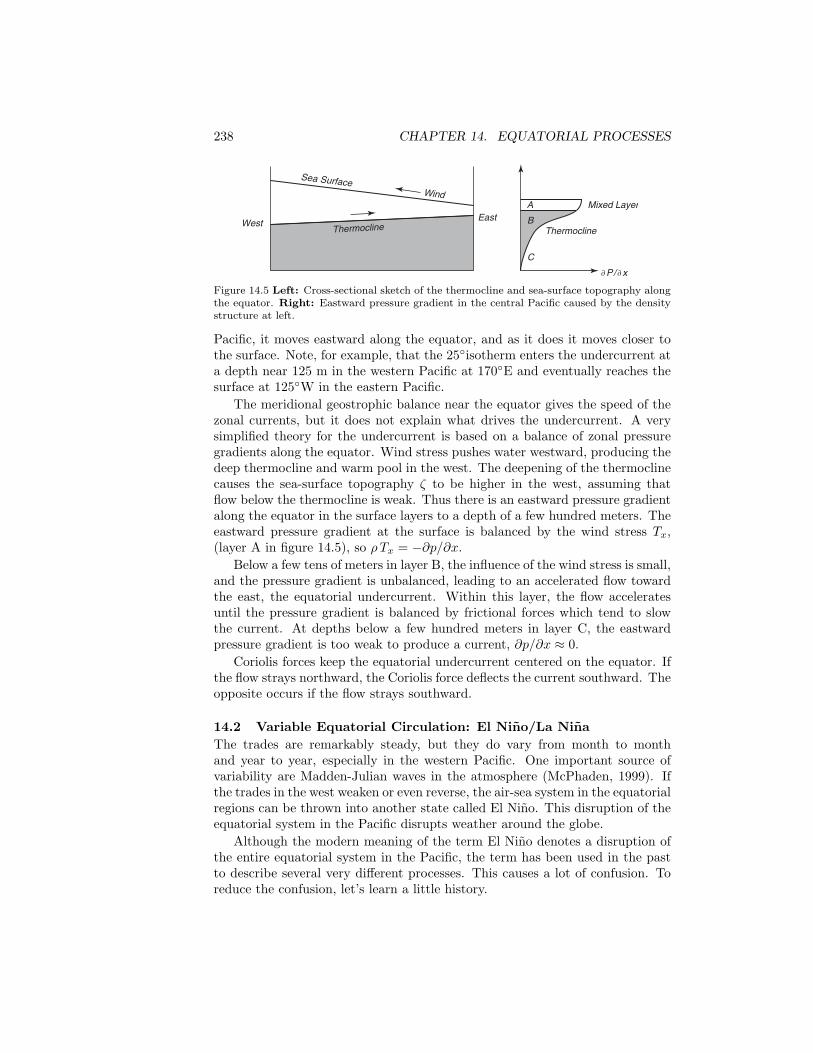
238 CHAPTER 14. EQUATORIAL PROCESSES
Sea SurfaceWind
C
A
BThermocline
Mixed Layer
∂P/∂x
EastWest
Thermocline
Figure 14.5 Left: Cross-sectional sketch of the thermocline and sea-surface topography alongthe equator. Right: Eastward pressure gradient in the central Pacific caused by the densitystructure at left.
Pacific, it moves eastward along the equator, and as it does it moves closer tothe surface. Note, for example, that the 25isotherm enters the undercurrent ata depth near 125 m in the western Pacific at 170E and eventually reaches thesurface at 125W in the eastern Pacific.
The meridional geostrophic balance near the equator gives the speed of thezonal currents, but it does not explain what drives the undercurrent. A verysimplified theory for the undercurrent is based on a balance of zonal pressuregradients along the equator. Wind stress pushes water westward, producing thedeep thermocline and warm pool in the west. The deepening of the thermoclinecauses the sea-surface topography ζ to be higher in the west, assuming thatflow below the thermocline is weak. Thus there is an eastward pressure gradientalong the equator in the surface layers to a depth of a few hundred meters. Theeastward pressure gradient at the surface is balanced by the wind stress Tx,(layer A in figure 14.5), so ρ Tx = −∂p/∂x.
Below a few tens of meters in layer B, the influence of the wind stress is small,and the pressure gradient is unbalanced, leading to an accelerated flow towardthe east, the equatorial undercurrent. Within this layer, the flow acceleratesuntil the pressure gradient is balanced by frictional forces which tend to slowthe current. At depths below a few hundred meters in layer C, the eastwardpressure gradient is too weak to produce a current, ∂p/∂x ≈ 0.
Coriolis forces keep the equatorial undercurrent centered on the equator. Ifthe flow strays northward, the Coriolis force deflects the current southward. Theopposite occurs if the flow strays southward.
14.2 Variable Equatorial Circulation: El Nino/La NinaThe trades are remarkably steady, but they do vary from month to monthand year to year, especially in the western Pacific. One important source ofvariability are Madden-Julian waves in the atmosphere (McPhaden, 1999). Ifthe trades in the west weaken or even reverse, the air-sea system in the equatorialregions can be thrown into another state called El Nino. This disruption of theequatorial system in the Pacific disrupts weather around the globe.
Although the modern meaning of the term El Nino denotes a disruption ofthe entire equatorial system in the Pacific, the term has been used in the pastto describe several very different processes. This causes a lot of confusion. Toreduce the confusion, let’s learn a little history.

14.2. EL NINO 239
A Little History Many years ago, way back in the 19th century, the term wasapplied to conditions off the coast of Peru. The following quote comes from theintroduction to Philander’s (1990) excellent book El Nino, La Nina, and theSouthern Oscillation:
In the year 1891, Senor Dr. Luis Carranza of the Lima GeographicalSociety, contributed a small article to the Bulletin of that Society, callingattention to the fact that a counter-current flowing from north to southhad been observed between the ports of Paita and Pacasmayo.
The Paita sailors, who frequently navigate along the coast in smallcraft, either to the north or the south of that port, name this counter-current the current of “El Nino” (the Child Jesus) because it has beenobserved to appear immediately after Christmas.
As this counter-current has been noticed on different occasions, andits appearance along the Peruvian coast has been concurrent with rains inlatitudes where it seldom if ever rains to any great extent, I wish, on thepresent occasion, to call the attention of the distinguished geographershere assembled to this phenomenon, which exercises, undoubtedly, a verygreat influence over the climatic conditions of that part of the world.—Senor Frederico Alfonso Pezet’s address to the Sixth International Geo-graphical Congress in Lima, Peru 1895.
The Peruvians noticed that in some years the El Nino current was strongerthan normal, it penetrated further south, and it is associated with heavy rainsin Peru. This occurred in 1891 when (again quoting from Philander’s book)
. . . it was then seen that, whereas nearly every summer here andthere there is a trace of the current along the coast, in that year it wasso visible, and its effects were so palpable by the fact that large deadalligators and trunks of trees were borne down to Pacasmayo from thenorth, and that the whole temperature of that portion of Peru sufferedsuch a change owing to the hot current that bathed the coast. . . . —SenorFrederico Alfonso Pezet.
. . . the sea is full of wonders, the land even more so. First of all thedesert becomes a garden . . . . The soil is soaked by the heavy downpour,and within a few weeks the whole country is covered by abundant pasture.The natural increase of flocks is practically doubled and cotton can begrown in places where in other years vegetation seems impossible.—FromMr. S.M. Scott & Mr. H. Twiddle quoted from a paper by Murphy, 1926.
The El Nino of 1957 was even more exceptional. So much so that it attractedthe attention of meteorologists and oceanographers throughout the Pacific basin.
By the fall of 1957, the coral ring of Canton Island, in the memory ofman ever bleak and dry, was lush with the seedlings of countless tropicaltrees and vines.
One is inclined to select the events of this isolated atoll as epitomizingthe year, for even here, on the remote edges of the Pacific, vast concertedshifts in the oceans and atmosphere had wrought dramatic change.
Elsewhere about the Pacific it also was common knowledge that theyear had been one of extraordinary climatic events. Hawaii had its first
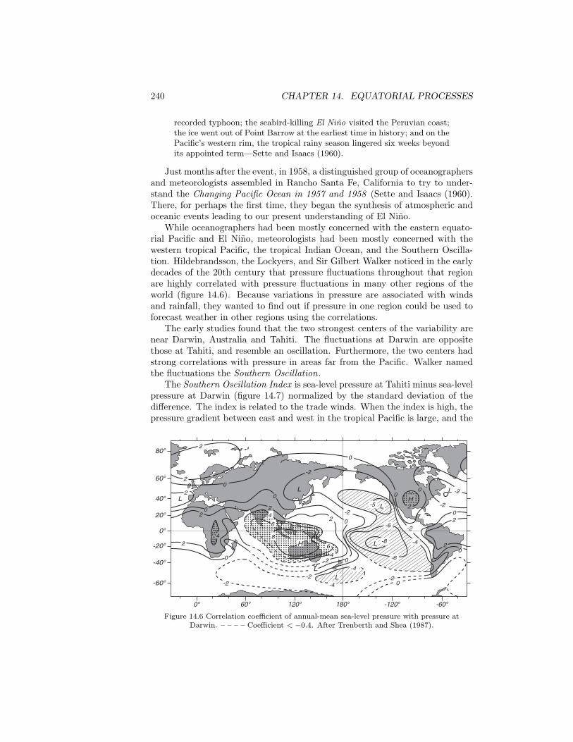
240 CHAPTER 14. EQUATORIAL PROCESSES
recorded typhoon; the seabird-killing El Nino visited the Peruvian coast;the ice went out of Point Barrow at the earliest time in history; and on thePacific’s western rim, the tropical rainy season lingered six weeks beyondits appointed term—Sette and Isaacs (1960).
Just months after the event, in 1958, a distinguished group of oceanographersand meteorologists assembled in Rancho Santa Fe, California to try to under-stand the Changing Pacific Ocean in 1957 and 1958 (Sette and Isaacs (1960).There, for perhaps the first time, they began the synthesis of atmospheric andoceanic events leading to our present understanding of El Nino.
While oceanographers had been mostly concerned with the eastern equato-rial Pacific and El Nino, meteorologists had been mostly concerned with thewestern tropical Pacific, the tropical Indian Ocean, and the Southern Oscilla-tion. Hildebrandsson, the Lockyers, and Sir Gilbert Walker noticed in the earlydecades of the 20th century that pressure fluctuations throughout that regionare highly correlated with pressure fluctuations in many other regions of theworld (figure 14.6). Because variations in pressure are associated with windsand rainfall, they wanted to find out if pressure in one region could be used toforecast weather in other regions using the correlations.
The early studies found that the two strongest centers of the variability arenear Darwin, Australia and Tahiti. The fluctuations at Darwin are oppositethose at Tahiti, and resemble an oscillation. Furthermore, the two centers hadstrong correlations with pressure in areas far from the Pacific. Walker namedthe fluctuations the Southern Oscillation.
The Southern Oscillation Index is sea-level pressure at Tahiti minus sea-levelpressure at Darwin (figure 14.7) normalized by the standard deviation of thedifference. The index is related to the trade winds. When the index is high, thepressure gradient between east and west in the tropical Pacific is large, and the
2
20
2
20
L 0
2
4
0
-2
8
6
4
H
-2
-4
-42
6
40
LL
L
2 0
-2
L
L-5
-6
-8 -4
-6
-20
H2
-2
0
0-2
-2
0
-2
0
0
2
22
L
-60o
-40o
0o
-20o
20o
40o
60o
80o
60o0o 120o -120o180o -60o
Figure 14.6 Correlation coefficient of annual-mean sea-level pressure with pressure atDarwin. – – – – Coefficient < −0.4. After Trenberth and Shea (1987).

14.2. EL NINO 241
Normalized Southern Oscillation Index
-4
-3
-2
-1
0
1
2
3
1950 1955 1960 1965 1970 1975 1980 1985 1990 1995 2000
Date
Nor
mal
ized
Inde
x
Figure 14.7 Normalized Southern Oscillation Index from 1951 to 1999. The normalized indexis sea-level pressure anomaly at Tahiti divided by its standard deviation minus sea-levelpressure anomaly at Darwin divided by its standard deviation then the difference is dividedby the standard deviation of the difference. The means are calculated from 1951 to 1980.Monthly values of the index have been smoothed with a 5-month running mean. Strong ElNino events occurred in 1957–58, 1965–66, 1972–73, 1982–83, 1997–98. Data from noaa.
trade winds are strong. When the index is negative trades, are weak.The connection between the Southern Oscillation and El Nino was made soon
after the Rancho Santa Fe meeting. Ichiye and Petersen (1963) and Bjerknes(1966) noticed the relationship between equatorial temperatures in the Pacificduring the 1957 El Nino and fluctuations in the trade winds associated with theSouthern Oscillation. The theory was further developed by Wyrtki (1975).
Because El Nino and the Southern Oscillation are so closely related, thephenomenon is often referred to as the El Nino–Southern Oscillation or enso.More recently, the oscillation is referred to as El Nino/La Nina, where La Ninarefers to the positive phase of the oscillation when trade winds are strong, andwater temperature in the eastern equatorial region is very cold.
Philander (1990) pointed out that each El Nino is unique, with differenttemperature, pressure, and rainfall patterns. Some are strong, others are weak.So, exactly what events deserve to be called El Nino? Recent studies based onthe coads data show that the best indicator of El Nino is sea-level pressureanomaly in the eastern equatorial Pacific from 4S to 4N and from 108Wto 98W (Harrison and Larkin, 1996). It correlates better with sea-surfacetemperature in the central Pacific than with the Southern-Oscillation Index.Thus the importance of the El Nino is not exactly proportional to the SouthernOscillation Index—the strong El Nino of 1957–58, has a weaker signal in figure7 than the weaker El Nino of 1965–66.
Trenberth (1997), based on discussions within the Climate Variability andPredictability program, recommends that those disruptions of the equatorialsystem in the Pacific shall be called an El Nino only when the 5-month run-ning mean of sea-surface temperature anomalies in the region 5N–5S, 120W–170W exceeds 0.4C for six months or longer.
So El Nino, which started life as a change in currents off Peru each Christmas,has grown into a giant. It now means a disruption of the ocean-atmosphere

242 CHAPTER 14. EQUATORIAL PROCESSES
system over the whole equatorial Pacific.
Theory of El Nino Wyrtki (1975) gives a clear, modern description of ElNino.
During the two years preceding El Nino, excessively strong southeasttrades are present in the central Pacific. These strong southeast tradesintensify the subtropical gyre of the South Pacific, strengthen the SouthEquatorial Current, and increase the east-west slope of sea level by build-ing up water in the western equatorial Pacific. As soon as the wind stressin the central Pacific relaxes, the accumulated water flows eastward, prob-ably in the form of an equatorial Kelvin wave. This wave leads to the ac-cumulation of warm water off Ecuador and Peru and to a depression of theusually shallow thermocline. In total, El Nino is the result of the responseof the equatorial Pacific to atmospheric forcing by the trade winds.
Sometimes the trades in the western equatorial Pacific not only weaken,they actually reverse direction for a few weeks to a month, producing westerlywind bursts that quickly deepen the thermocline there. The deepening of thethermocline launches an eastward propagating Kelvin wave and a westwardpropagating Rossby wave. (If you are asking, What are Kelvin and Rossbywaves? I will answer that in a minute. So please be patient.)
The Kelvin wave deepens the thermocline as it moves eastward, and it carrieswarm water eastward. Both processes cause a deepening of the mixed layer inthe eastern equatorial Pacific a few months after the wave is launched in thewestern Pacific. The deeper thermocline in the east leads to upwelling of warmwater, and the surface temperatures offshore of Ecuador and Peru warms by 2–4. The warm water reduces the temperature contrast between east and west,further reducing the trades and hastening the development of El Nino.
With time, the warm pool spreads east, eventually extending as far as 140W(figure 14.8). Plus, water warms in the east along the equator due to upwellingof warm water, and to reduced advection of cold water from the east due toweaker trade winds.
The warm waters along the equator in the east cause the areas of heavy rainto move eastward from Melanesia and Fiji to the central Pacific. Essentially,a major source of heat for the atmospheric circulation moves from the west tothe central Pacific, and the whole atmosphere responds to the change. Bjerknes(1972), describing the interaction between the ocean and the atmosphere overthe eastern equatorial Pacific concluded:
In the cold ocean case (1964) the atmosphere has a pronounced stablelayer between 900 and 800 mb, preventing convection and rainfall, and inthe warm case (1965) the heat supply from the ocean eliminates the atmo-spheric stability and activates rainfall. . . . A side effect of the widespreadwarming of the tropical belt of the atmosphere shows up in the increaseof exchange of angular momentum with the neighboring subtropical belt,whereby the subtropical westerly jet strengthens . . . The variability ofthe heat and moisture supply to the global atmospheric thermal enginefrom the equatorial Pacific can be shown to have far-reaching large-scaleeffects.

14.2. EL NINO 243
0.2
0.2
0.2
0.20.4
0.4
0.40.4
0.4
0.40.4
0.2-0.2
0
0
-0.2
00
00
0
0
0
0
0 00.2
-0.2
-0.4-0.4
-0.2
-0.6
0.2 0.4 0.6
0.6
0.60.8
0.20.2
-0.2
-0.2
-0.2
0.20.6
0.2
-0.2
0.20.4
0.4
-0.2
0.4
-0.2 -0.2-0.4
0.60 0
0
0
00
0 -0.2
-0.2
1.61.4 1.2
1.0
0.2
0
0
00.2
0.2
0
0
0-0.2 -0.2
-0.4 -0.2
-0.2
-0.4
-0.4
0.4-0.6
1.0
-0.2
1.2
0
0.40.6
0.2
1.0
0.2
0.8
0.81.0
0
-0.2
1.41.2
-0.2
-0.2
0.2
0.20.4 0.4
0.2
0 0.2
0.20 00.2-0.2
0
0
0
00
00.6
0.4 0.4
0.80.6
0.8
0.60.4
0.8
1.0
(a) March-May
(b) August-October
(b) December-February
(d) May-July
30o
20o
10o
0o
-10o
-20o
-30o
100o 120o 140o 160o 180o -160o -140o -120o -100o -80o
30o
20o
10o
0o
-10o
-20o
-30o
100o 120o 140o 160o 180o -160o -140o -120o -100o -80o
30o
20o
10o
0o
-10o
-20o
-30o
100o 120o 140o 160o 180o -160o -140o -120o -100o -80o
30o
20o
10o
0o
-10o
-20o
-30o
100o 120o 140o 160o 180o -160o -140o -120o -100o -80o
Figure 14.8 Anomalies of sea-surface temperature (in C) during a typical El Nino obtainedby averaging data from El Ninos between 1950 and 1973. Months are after the onset of theevent. After Rasmusson and Carpenter (1982).

244 CHAPTER 14. EQUATORIAL PROCESSES
It is these far reaching events that make El Nino so important. Few peoplecare about warm water off Peru around Christmas, many care about globalchanges the weather. El Nino is important because of its influence on theatmosphere.
After the Kelvin wave reaches the coast of Ecuador, part is reflected as anwestward propagating Rossby wave, and part propagates north and south asa coastal trapped Kelvin wave carrying warm water to higher latitudes. Forexample, during the 1957 El Nino, the northward propagating Kelvin waveproduced unusually warm water off shore of California, and it eventually reachedAlaska. This warming of the west coast of North America further influencesclimate in North America, especially in California.
As the Kelvin wave moves along the coast, it forces other Rossby waveswhich move west across the Pacific with a velocity that depends on the latitude(14.4). The velocity is very slow at mid to high latitudes and fastest on theequator. There the reflected wave moves back as a deepening of the thermo-cline, reaching the central equatorial Pacific a year later. In a similar way, thewestward propagating Rossby wave launched at the start of the El Nino in thewest, reflects off Asia and returns to the central equatorial Pacific as a Kelvinwave, again about a year later.
El Nino ends when the Rossby waves reflected from Asia and Ecuador meetin the central Pacific about a year after the onset of El Nino (Picaut, Masia, anddu Penhoat, 1997). The waves push the warm pool at the surface toward thewest. At the same time, the Rossby wave reflected from the western boundarycauses the thermocline in the central Pacific to become shallower when thewaves reaches the central Pacific. Then any strengthening of the trades causesupwelling of cold water in the east, which increases the east-west temperaturegradient, which increases the trades, which increases the upwelling (Takayabu etal 1999). The system is then thrown into the La Nina state with strong trades,and a very cold tongue along the equator in the east.
La Nina tends to last longer than El Nino, and the cycle from La Nina to ElNino and back takes about three years. The cycle isn’t exact. El Nino comesback at intervals from 2-7 years, with an average near four years (figure 14.7).
Equatorial Kelvin and Rossby Waves Kelvin and Rossby waves are theocean’s way of adjusting to changes in forcing such as westerly wind bursts.The adjustment occurs as waves of current and sea level that are influenced bygravity, Coriolis force f , and the north-south variation of Coriolis force ∂f/∂y =β. There are many kinds of these waves with different spatial distributions,frequencies, wavelengths, speed and direction of propagation. If gravity and fare the restoring forces, the waves are called Kelvin and Poincare waves. If β isthe restoring force, the waves are called planetary waves. One important typeof planetary wave is the Rossby wave.
Two types of waves are especially important for El Nino: internal Kelvinwaves and Rossby waves. Both waves can have modes that are confined toa narrow, north-south region centered on the equator. These are equatoriallytrapped waves. Both exist in slightly different forms at higher latitudes.
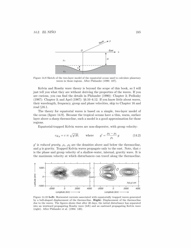
14.2. EL NINO 245
H
y
x
ρ1
ρ2
h
O East
North
Figure 14.9 Sketch of the two-layer model of the equatorial ocean used to calculate planetarywaves in those regions. After Philander (1990: 107).
Kelvin and Rossby wave theory is beyond the scope of this book, so I willjust tell you what they are without deriving the properties of the waves. If youare curious, you can find the details in Philander (1990): Chapter 3; Pedlosky(1987): Chapter 3; and Apel (1987): §6.10–6.12. If you know little about waves,their wavelength, frequency, group and phase velocities, skip to Chapter 16 andread §16.1.
The theory for equatorial waves is based on a simple, two-layer model ofthe ocean (figure 14.9). Because the tropical oceans have a thin, warm, surfacelayer above a sharp thermocline, such a model is a good approximation for thoseregions.
Equatorial-trapped Kelvin waves are non-dispersive, with group velocity:
cKg = c ≡√
g′H; where g′ =ρ2 − ρ1
ρ1g (14.2)
g′ is reduced gravity , ρ1, ρ2 are the densities above and below the thermocline,and g is gravity. Trapped Kelvin waves propagate only to the east. Note, that cis the phase and group velocity of a shallow-water, internal, gravity wave. It isthe maximum velocity at which disturbances can travel along the thermocline.
.3
2.1.3
2.1
h(x,y) cm
Latit
ude
(km
)
1000
-1000
Longitute (km)
-2000 0 2000 4000
0
-2000 0 2000 4000
Equator
Longitute (km)
Figure 14.10 Left: Horizontal currents associated with equatorially trapped waves generatedby a bell-shaped displacement of the thermocline. Right: Displacement of the thermoclinedue to the waves. The figures shows that after 20 days, the initial disturbance has separatedinto an westward propagating Rossby wave (left) and an eastward propagating Kelvin wave(right). After Philander et al. (1984: 120).

246 CHAPTER 14. EQUATORIAL PROCESSES
Typical values of the quantities in (14.2) are:
ρ2 − ρ1
ρ1= 0.003; H = 150 m; c = 2.1 m/s
At the equator, Kelvin waves propagate eastward at speeds of up to 3 m/s, andthey cross the Pacific in a few months. Currents associated with the wave areeverywhere eastward with north-south component (figure 14.10).
Kelvin waves can also propagate poleward as a trapped wave along an eastcoast of an ocean basin. Their group velocity is also given by (14.3), and theyare confined to a coastal zone with width x = c/ (β y)
The important Rossby waves on the equator have frequencies much less thanthe Coriolis frequency. They can travel only to the west. The group velocity is:
cRg = − c
(2n + 1); n = 1, 2, 3, . . . (14.3)
The fastest wave travels westward at a velocity near 0.8 m/s. The currentsassociated with the wave are almost in geostrophic balance in two counter-rotating eddies centered on the equator (figure 14.10).
Away from the equator, low-frequency, long-wavelength Rossby waves alsotravel only to the west, and the currents associated with the waves are againalmost in geostrophic balance. Group velocity depends strongly on latitude:
cRg = −β g′ H
f2(14.4)
The wave dynamics in the equatorial regions differ markedly from wave dy-namics at mid-latitudes. The baroclinic waves are much faster, and the response
Jun(0)-Sep(0)
Sep(0)-May(+)
Oct(0)-Dec(0)
Nov(0)-May(+)
Jun(0)-Nov(0)
Sep(0)-Mar(+)
Mar(0)-Feb(+)
May(0)-Oct(0)
Nov(0)-May(+)
May(0)-Apr(+)
Apr(0)-Mar(+)Jul(0)-Jun(+)
Apr(0)-Oct(0)
Insufficientstation datafor analysis
Jul(0)-Mar(+)
Oct(0)-Mar(+)
Nov(0)-Feb(+)
0o 40o 80o 120o 160o -160o -120o -80o -40o
60o
40o
20o
0o
-20o
-40o
-60o
180o
Figure 14.11 Sketch of regions receiving enhanced rain (dashed lines) or drought (solid lines)during an El Nino event. (0) indicates that rain changed during the year in which El Ninobegan, (+)indicates that rain changed during the year after El Nino began. After Ropelewskiand Halpert (1987).

14.3. EL NINO TELECONNECTIONS 247
of the ocean to changes in wind forcing is also much faster than at mid-latitudes.For the planetary waves confined to the equator, we can speak of an equatorialwave guide.
Now, let’s return to El Nino and its “far-reaching large-scale effects.”
14.3 El Nino Teleconnections
Teleconnections are statistically significant correlations between weather eventsthat occur at different places on the Earth. Figure 14.11 shows the dominantglobal teleconnections associated with the El Nino/Southern Oscillation enso.It shows that enso is an atmospheric perturbation influencing the entire Pacific.
The influence of enso is through its influence on convection in the equatorialPacific. As the area of heavy rain moves east, it perturbs atmospheric pressure(figure 14.12) and influences the position of the jet stream at higher latitudes.This sequence of events leads to some predictability of weather patterns a sea-son in advance over North America, Brazil, Australia, South Africa and otherregions.
The enso perturbations to mid-latitude and tropical weather systems leadsto dramatic changes in rainfall in some regions (figure 14.11). As the convectiveregions migrate east along the equator, they bring rain to the normally arid,central-Pacific islands. The lack of rain the the western Pacific leads to droughtin Indonesia and Australia.
EQ
NP GM
Figure 14.12 Changing patterns of convection in the equatorial Pacific during an El Nino,set up a pattern of pressure anomalies in the atmosphere (solid lines) which influence theextratropical atmosphere. After Rasmusson and Wallace (1983).
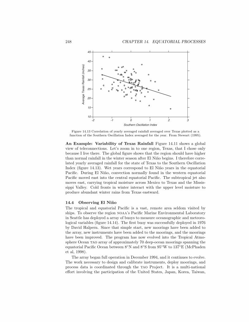
248 CHAPTER 14. EQUATORIAL PROCESSES
-2 -1 0 1 2 3
Southern Oscillation Index
Ave
rage
Tex
as R
ainf
all (
inch
es)
45
40
35
30
25
20
15
10
Figure 14.13 Correlation of yearly averaged rainfall averaged over Texas plotted as afunction of the Southern Oscillation Index averaged for the year. From Stewart (1995).
An Example: Variability of Texas Rainfall Figure 14.11 shows a globalview of teleconnections. Let’s zoom in to one region, Texas, that I chose onlybecause I live there. The global figure shows that the region should have higherthan normal rainfall in the winter season after El Nino begins. I therefore corre-lated yearly averaged rainfall for the state of Texas to the Southern OscillationIndex (figure 14.13). Wet years correspond to El Nino years in the equatorialPacific. During El Nino, convection normally found in the western equatorialPacific moved east into the central equatorial Pacific. The subtropical jet alsomoves east, carrying tropical moisture across Mexico to Texas and the Missis-sippi Valley. Cold fronts in winter interact with the upper level moisture toproduce abundant winter rains from Texas eastward.
14.4 Observing El NinoThe tropical and equatorial Pacific is a vast, remote area seldom visited byships. To observe the region noaa’s Pacific Marine Environmental Laboratoryin Seattle has deployed a array of buoys to measure oceanographic and meteoro-logical variables (figure 14.14). The first buoy was successfully deployed in 1976by David Halpern. Since that simple start, new moorings have been added tothe array, new instruments have been added to the moorings, and the mooringshave been improved. The program has now evolved into the Tropical Atmo-sphere Ocean tao array of approximately 70 deep-ocean moorings spanning theequatorial Pacific Ocean between 8N and 8S from 95W to 137E (McPhadenet al, 1998).
The array began full operation in December 1994, and it continues to evolve.The work necessary to design and calibrate instruments, deploy moorings, andprocess data is coordinated through the tao Project. It is a multi-nationaleffort involving the participation of the United States, Japan, Korea, Taiwan,
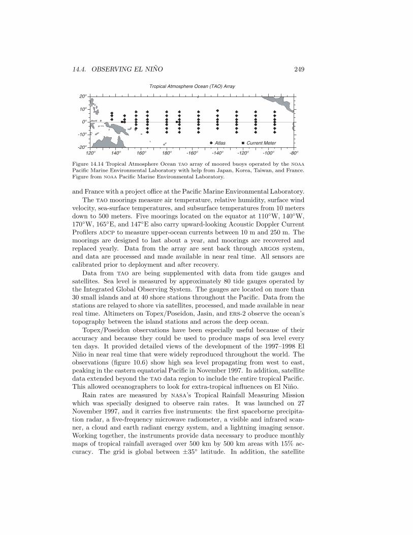
14.4. OBSERVING EL NINO 249
Tropical Atmosphere Ocean (TAO) Array
Atlas Current Meter
180o160o140o120o -160o -140o -120o -100o -80o
20o
0o
10o
-10o
-20o
Figure 14.14 Tropical Atmosphere Ocean tao array of moored buoys operated by the noaaPacific Marine Environmental Laboratory with help from Japan, Korea, Taiwan, and France.Figure from noaa Pacific Marine Environmental Laboratory.
and France with a project office at the Pacific Marine Environmental Laboratory.The tao moorings measure air temperature, relative humidity, surface wind
velocity, sea-surface temperatures, and subsurface temperatures from 10 metersdown to 500 meters. Five moorings located on the equator at 110W, 140W,170W, 165E, and 147E also carry upward-looking Acoustic Doppler CurrentProfilers adcp to measure upper-ocean currents between 10 m and 250 m. Themoorings are designed to last about a year, and moorings are recovered andreplaced yearly. Data from the array are sent back through argos system,and data are processed and made available in near real time. All sensors arecalibrated prior to deployment and after recovery.
Data from tao are being supplemented with data from tide gauges andsatellites. Sea level is measured by approximately 80 tide gauges operated bythe Integrated Global Observing System. The gauges are located on more than30 small islands and at 40 shore stations throughout the Pacific. Data from thestations are relayed to shore via satellites, processed, and made available in nearreal time. Altimeters on Topex/Poseidon, Jasin, and ers-2 observe the ocean’stopography between the island stations and across the deep ocean.
Topex/Poseidon observations have been especially useful because of theiraccuracy and because they could be used to produce maps of sea level everyten days. It provided detailed views of the development of the 1997–1998 ElNino in near real time that were widely reproduced throughout the world. Theobservations (figure 10.6) show high sea level propagating from west to east,peaking in the eastern equatorial Pacific in November 1997. In addition, satellitedata extended beyond the tao data region to include the entire tropical Pacific.This allowed oceanographers to look for extra-tropical influences on El Nino.
Rain rates are measured by nasa’s Tropical Rainfall Measuring Missionwhich was specially designed to observe rain rates. It was launched on 27November 1997, and it carries five instruments: the first spaceborne precipita-tion radar, a five-frequency microwave radiometer, a visible and infrared scan-ner, a cloud and earth radiant energy system, and a lightning imaging sensor.Working together, the instruments provide data necessary to produce monthlymaps of tropical rainfall averaged over 500 km by 500 km areas with 15% ac-curacy. The grid is global between ±35 latitude. In addition, the satellite

250 CHAPTER 14. EQUATORIAL PROCESSES
data are used to measure latent heat released to the atmosphere by rain, thusproviding continuous monitoring of heating of the atmosphere in the tropics.
14.5 Forecasting El NinoThe importance of El Nino to global weather patterns has led to many schemesfor forecasting events in the equatorial Pacific. Several generations of modelshave been produced, but the skill of the forecasts has not always increased.Models worked well for a few years, then failed. Failure was followed by im-proved models, and the cycle continued. Thus, the best models in 1991 failedto predict weak El Ninos in 1993 and 1994 (Ji, Leetmaa, and Kousky, 1996).The best model of the mid 1990s failed to predict the onset of the strong ElNino of 1997-1998 although a new model developed by the National Centersfor Environmental Prediction made the best forecast of the development of theevent. In general, the more sophisticated the model, the better the forecasts(Kerr, 1998).
The following recounts some of the more recent work to improve the fore-casts. For simplicity, I describe the technique used by the National Centers forEnvironmental Prediction (Ji, Behringer, and Leetmaa, 1998). But Chen et al.(1995), Latif et al. (1993), and Barnett et al. (1993), among others, have alldeveloped useful prediction models.
Atmospheric Models How well can we model atmospheric processes overthe Pacific? To help answer the question, the World Climate Research Pro-gram’s Atmospheric Model Intercomparison Project (Gates, 1992) comparedoutput from 30 different atmospheric numerical models for 1979 to 1988. TheVariability in the Tropics: Synoptic to Intraseasonal Timescales subproject isespecially important because it documents the ability of 15 atmospheric general-circulation models to simulate the observed variability in the tropical atmo-sphere (Slingo et al. 1995). The models included several operated by gov-ernment weather forecasting centers, including the model used for day-to-dayforecasts by the European Center for Medium-Range Weather Forecasts.
The first results indicate that none of the models were able to duplicate allimportant interseasonal variability of the tropical atmosphere on timescales of2 to 80 days. Models with weak intraseasonal activity tended to have a weakannual cycle. Most models seemed to simulate some important aspects of theinterannual variability including El Nino. The length of the time series was,however, too short to provide conclusive results on interannual variability.
The results of the substudy imply that numerical models of the atmosphericgeneral circulation need to be improved if they are to be used to study tropicalvariability and the response of the atmosphere to changes in the tropical ocean.
Oceanic Models Our ability to understand El Nino also depends on ourability to model the oceanic circulation in the equatorial Pacific. Because themodels provide the initial conditions used for the forecasts, they must be able toassimilate up-to-date measurements of the Pacific along with heat fluxes and sur-face winds calculated from the atmospheric models. The measurements includesea-surface winds from scatterometers and moored buoys, surface temperature

14.5. FORECASTING EL NINO 251
from the optimal-interpolation data set (see §6.6), subsurface temperatures frombuoys and xbts, and sea level from altimetry and tide-gauges on islands.
Ji, Behringer, and Leetmaa (1998) at the National Centers for Environ-mental Prediction have modified the Geophysical Fluid Dynamics Laboratory’sModular Ocean Model for use in the tropical Pacific (see §15.4 for more infor-mation about this model). It’s domain is the Pacific between 45S and 55Nand between 120E and 70W. The zonal resolution is 1.5. The meridionalresolution is 1/3 within 10 of the equator, increasing smoothly to 1 pole-ward of 20 latitude. It has 28 vertical levels, with 18 in the upper 400 m toresolve the mixed layer and thermocline. The model is driven by mean windsfrom Hellerman and Rosenstein (1983), anomalies in the wind field from FloridaState University, and mean heat fluxes from Oberhuber (1988). It assimilatessubsurface temperature from the tao array and xbts, and surface temperaturesfrom the monthly optimal-interpolation data set (Reynolds and Smith, 1994).
The output of the model is an ocean analysis, the density and current fieldthat best fits the data used in the analysis (figures 14.3 and 14.4). This is usedto drive a coupled ocean-atmosphere model to produce forecasts.
Coupled Models Coupled models are separate atmospheric and oceanicmodels that pass information through their common boundary at the sea sur-face, thus coupling the two calculations. The coupling can be one way, from theatmosphere, or two way, into and out of the ocean. In the scheme used by thenoaa National Centers for Environmental Prediction the ocean model is thesame Modular Ocean Model described above. It is coupled to a low-resolutionversion of the global, medium-range forecast model operated by the NationalCenters (Kumar, Leetmaa, and Ji, 1994). Anomalies of wind stress, heat, andfresh-water fluxes calculated from the atmospheric model are added to the meanannual values of the fluxes, and the sums are used to drive the ocean model.Sea-surface temperature calculated from the ocean model is used to drive theatmospheric model from 15N to 15S.
As computer power decreases in cost, the models are becoming ever morecomplex. The trend is to global coupled models able to include other coupledocean-atmosphere systems in addition to enso. We return to the problem in§15.7 where I describe global coupled models.
Forecasts In general, the coupled ocean-atmosphere models produce thebest forecasts. The forecasts include not only events in the Pacific but also theglobal consequences of El Nino. The forecasts are judged two ways:
1. Using the correlation between the area-averaged sea-surface-temperatureanomalies from the model and the observed temperature anomalies in theeastern equatorial Pacific. The area is usually from 170W to 120Wbetween 5S and 5N. Useful forecasts have correlations exceeding 0.6.
2. Using the root-mean-square difference between the observed and predictedsea-surface temperature in the same area.
Forecasts made from the National-Centers coupled model were useful up toone year in advance when run using data from 1981 to 1995. The predictedsea-surface temperature was less than 1C for the forecasts. Forecasts had

252 CHAPTER 14. EQUATORIAL PROCESSES
less skill for the period from 1992 to 1995, the period with weak warm events.The forecasts were useful for periods of less than eight months, although thetemperature error was less than 0.7C. The most accurate forecasts were thosethat started during the northern hemisphere warm period from May throughSeptember. Forecasts made in November through January were significantlyless accurate (Ji, Behringer, and Leetmaa, 1998).
In conclusion, it appears that coupled ocean-atmosphere models driven withaccurate atmospheric and oceanic data can produce useful forecasts of the de-velopment El Nino even if they often miss the onset of the event.
14.6 Important Concepts1. Equatorial processes are important because heat released by rain in the
equatorial region helps drives much of the atmospheric circulation.
2. Equatorial currents redistribute heat. The interannual variability of cur-rents and temperatures in the equatorial Pacific modulates the oceanicforcing of the atmosphere.
3. Changes in equatorial dynamics cause changes in atmospheric circulationby changing the location of rain in tropical Pacific and therefore the loca-tion of the major heat source driving the atmospheric circulation.
4. El Nino causes the biggest changes in equatorial dynamics. During ElNino, trade-winds weaken in the western Pacific, the thermocline becomesless deep in the west. This drives a Kelvin wave eastward along the equa-tor, which deepens the thermocline in the eastern Pacific. The warm poolin the west moves eastward toward the central Pacific, and the intensetropical rain areas move with the warm pool.
5. As a result of El Nino, drought occurs in the Indonesian area and northernAustralia, and floods occur in western, tropical South America. Variationsin the atmospheric circulation influence more distant areas through tele-connections.
6. Forecasts of El Nino are made using coupled ocean-atmospheric numeri-cal models. Forecasts appear to have useful accuracy for 3–6 months inadvance, mostly after the onset of El Nino.

Chapter 15
Numerical Models
We saw earlier that analytic solutions to the equations of motion are difficultor impossible to obtain for typical oceanic flows. The problem is due to thenon-linear terms, turbulence, and the need for realistic shapes for the sea floorand coastlines. We have also seen how difficult it is to describe the oceanfrom measurements. Satellites can observe some processes almost everywhereevery few days. But they observe only some processes, and only near or atthe surface. Ships can measure more variables, and deeper into the water, butthe measurements are sparse. Hence, numerical models provide the only useful,global view of ocean currents. Let’s look at the accuracy and validity of themodels, keeping in mind that although they are only models, they provide aremarkably detailed and realistic view of the ocean.
15.1 Introduction–Some Words of CautionNumerical models of ocean currents have many advantages. They simulate flowsin realistic ocean basins with a realistic sea floor. They include the influenceof viscosity and non-linear dynamics. And they can calculate possible futureflows in the ocean. Perhaps, most important, they interpolate between sparseobservations of the ocean produced by ships, drifters, and satellites.
Numerical models are not without problems. “There is a world of differencebetween the character of the fundamental laws, on the one hand, and the natureof the computations required to breathe life into them, on the other”—Berlinski(1996). The models can never give complete descriptions of the oceanic flowseven if the equations are integrated accurately. The problems arise from severalsources.
Discrete equations are not the same as continuous equations. In Chapter 7we wrote down the differential equations describing the motion of a continuousfluid. Numerical models use algebraic approximations to the differential equa-tions. We assume that the ocean basins are filled with a grid of points, andtime moves forward in tiny steps. The value of the current, pressure, tempera-ture, and salinity are calculated from their values at nearby points and previoustimes. Ian Stewart (1992), a noted mathematician, points out that
253

254 CHAPTER 15. NUMERICAL MODELS
Discretization is essential for computer implementation and cannot be dis-pensed with. The essence of the difficulty is that the dynamics of discretesystems is only loosely related to that of continuous systems—indeed thedynamics of discrete systems is far richer than that of their continuouscounterparts—and the approximations involved can create spurious solu-tions.
Calculations of turbulence are difficult. Numerical models provide informa-tion only at grid points of the model. They provide no information about theflow between the points. Yet, the ocean is turbulent, and any oceanic modelcapable of resolving the turbulence needs grid points spaced millimeters apart,with time steps of milliseconds.
Practical ocean models have grid points spaced tens to hundreds of kilome-ters apart in the horizontal, and tens to hundreds of meters apart in the vertical.This means that turbulence cannot be calculated directly, and the influence ofturbulence must be parameterized. Holloway (1994) states the problem suc-cinctly:
Ocean models retain fewer degrees of freedom than the actual ocean(by about 20 orders of magnitude). We compensate by applying ‘eddy-viscous goo’ to squash motion at all but the smallest retained scales.(We also use non-conservative numerics.) This is analogous to placing apartition in a box to prevent gas molecules from invading another regionof the box. Our oceanic models cannot invade most of the real oceanicdegrees of freedom simply because the models do not include them.
Given that we cannot do things ‘right’, is it better to do nothing?That is not an option. ‘Nothing’ means applying viscous goo and wishingfor the ever bigger computer. Can we do better? For example, can weguess a higher entropy configuration toward which the eddies tend todrive the ocean (that tendency to compete with the imposed forcing anddissipation)?
By “degrees of freedom” Holloway means all possible motions from the small-est waves and turbulence to the largest currents. Let’s do a simple calculation.We know that the ocean is turbulent with eddies as small as a few millimeters.To completely describe the ocean we need a model with grid points spaced 1mm apart and time steps of about 1 ms. The model must therefore have 360×180× (111 km/degree)2×1012 (mm/km)2× 3 km ×106 (mm/km) = 2.4×1027
data points for a 3 km deep ocean covering the globe. The global Parallel OceanProgram Model described in the next section has 2.2 × 10⁷ points. So we need1020 times more points to describe the real ocean. These are the missing 1020
degrees of freedom.Practical models must be simpler than the real ocean. Models of the ocean
must run on available computers. This means oceanographers further simplifytheir models. We use the hydrostatic and Boussinesq approximations, and weoften use equations integrated in the vertical, the shallow-water equations (Haid-vogel and Beckmann, 1999: 37). We do this because we cannot yet run the mostdetailed models of oceanic circulation for thousands of years to understand therole of the ocean in climate.

15.2. NUMERICAL MODELS IN OCEANOGRAPHY 255
Numerical code has errors. Do you know of any software without bugs?Numerical models use many subroutines each with many lines of code whichare converted into instructions understood by processors using other softwarecalled a compiler. Eliminating all software errors is impossible. With carefultesting, the output may be correct, but the accuracy cannot be guaranteed.Plus, numerical calculations cannot be more accurate than the accuracy of thefloating-point numbers and integers used by the computer. Round-off errors can-not be ignored. Lawrence et al (1999), examining the output of an atmosphericnumerical model found an error in the code produced by the fortran-90 com-piler used on the cray Research supercomputer used to run the code. Theyalso found round-off errors in the concentration of tracers calculated from themodel. Both errors produced important errors in the output of the model.
Summary Despite these many sources of error, most are small in practice.Numerical models of the ocean are giving the most detailed and complete viewsof the circulation available to oceanographers. Some of the simulations containunprecedented details of the flow. I included the words of warning not to leadyou to believe the models are wrong, but to lead you to accept the output witha grain of salt.
15.2 Numerical Models in OceanographyNumerical models are used for many purposes in oceanography. For our purposewe can divide models into two classes:
Mechanistic models are simplified models used for studying processes. Be-cause the models are simplified, the output is easier to interpret than outputfrom more complex models. Many different types of simplified models have beendeveloped, including models for describing planetary waves, the interaction ofthe flow with sea-floor features, or the response of the upper ocean to the wind.These are perhaps the most useful of all models because they provide insightinto the physical mechanisms influencing the ocean. The development and useof mechanistic models is, unfortunately, beyond the scope of this book.
Simulation models are used for calculating realistic circulation of oceanicregions. The models are often very complex because all important processes areincluded, and the output is difficult to interpret. Let’s look at a few of the morewidely used models.
15.3 Simulation ModelsThe first simulation models were developed by Kirk Bryan and Michael Cox atthe Geophysical Fluid Dynamics laboratory in Princeton. Their model (Bryan,1969) calculated the 3-dimensional flow in the ocean using the continuity andmomentum equation with the hydrostatic and Boussinesq approximations anda simplified equation of state. Such models are called primitive equation modelsbecause they use the most basic, or primitive form of the equations of motion.The equation of state allows the model to calculate changes in density dueto fluxes of heat and water through the sea surface, so the model includesthermodynamic processes.

256 CHAPTER 15. NUMERICAL MODELS
The Bryan-Cox model used large horizontal and vertical viscosity and diffu-sion to eliminate turbulent eddies having diameters smaller about 500 km, whichis a few grid points in the model. It also had complex coastlines, smoothed sea-floor features, and a rigid lid.
The rigid lid was necessary for eliminating ocean-surface waves, such as tidesand tsunamis which move far too fast for the coarse time steps used by all sim-ulation models. The rigid lid has, however, disadvantages. Islands substantiallyslow the computation, and the sea-floor features must be smoothed to eliminatesteep gradients.
The first simulation model was regional. It was quickly followed by a globalmodel (Cox, 1975) with a horizontal resolution of 2 and with 12 levels in thevertical. The model ran far too slowly even on the fastest computers of the day,but it laid the foundation for more recent models. The coarse spatial resolutionrequired that the model have large values for viscosity, and even regional modelswere too viscous to have realistic western boundary currents or mesoscale eddies.
Since those times, the goal has been to produce models with ever finer reso-lution. The hope was that if the resolution is sufficiently fine, the output will besufficiently realistic. Computer technology is changing rapidly, and models areevolving rapidly. The output from the most recent models of the North Atlantic,which have resolution of 0.1 look very much like the real ocean (Smith et al.2000). Models of other areas show previously unknown currents near Australiaand in the South Atlantic. Let’s look at a few typical and widely used models.
15.4 Primitive-Equation ModelsThe Bryan-Cox models evolved into many, widely used models which are pro-viding impressive views of the global ocean circulation. The models includethe influence of heat and water fluxes, eddy dynamics, and the meridional-overturning circulation. The models range in complexity from those that canrun on desktop workstations to those that require the world’s fastest computers.Semtner (1995) gives a good summary of present results from computers withmultiple, parallel processors.
Eddy-admitting, primitive-equation models have sufficient horizontal res-olution that they produce mesoscale eddies. The resolution of these models is afew tenths of a degree of latitude and longitude, which is sufficient to resolve thelargest eddies, those with diameter larger than two to three times the distancebetween grid points, such as those seen in figures 11.10, 11.11, and 15.2. Verti-cal resolution is typically around 30 vertical levels. The models include realisticcoasts and bottom features. The models are possible thanks to the developmentof fast, parallel processors with large memory. To obtain high vertical and hori-zontal resolution, the models require more than a million grid points. Typicallythey can simulate the global oceanic circulation for several decades.
Geophysical Fluid Dynamics Laboratory Modular Ocean Model MOM is per-haps the most widely used model growing out of the original Bryan-Cox code. Itconsists of a large set of modules that can be configured to run on many differentcomputers to model many different aspects of the circulation. The source code

15.4. PRIMITIVE-EQUATION MODELS 257
is open and free, and it is in the public domain. The model is widely use forclimate studies and and for studying the ocean’s circulation over a wide rangeof space and time scales (Pacanowski and Griffies, 1999).
Because mom is used to investigate processes which cover a wide range oftime and space scales, the code and manual are lengthy. However, it is farfrom necessary for the typical ocean modeler to become acquainted withall of its aspects. Indeed, mom can be likened to a growing city with manydifferent neighborhoods. Some of the neighborhoods communicate withone another, some are mutually incompatible, and others are basicallyindependent. This diversity is quite a challenge to coordinate and support.Indeed, over the years certain “neighborhoods” have been jettisoned orgreatly renovated for various reasons.—Pacanowski and Griffies.
The model uses the momentum equations, equation of state, and the hydro-static and Boussinesq approximations. Subgrid-scale motions are reduced byuse of eddy viscosity. Version 3 of the model has a free surface, realistic bottomfeatures, and many types of mixing including horizontal mixing along surfacesof constant density. Plus, it can be coupled to atmospheric models.
Semtner and Chervin’s Global Model was perhaps the first, global, eddy-admitting model based on the Bryan-Cox models (Semtner and Chervin, 1988).It has much in common with the Modular Ocean Model (Semtner helped writethe mom code), and it provided the first high resolution view of ocean dynamics.It has a resolution of 0.5 × 0.5 with 20 levels in the vertical. It has simpleeddy viscosity, which varies with scale. And it does not allow static instability.In contrast with earlier models, it is global, excluding only the Arctic Sea, itincludes the largest turbulent eddies, and it has realistic bottom features andcoastlines.
The model was started from rest with values of vertical density from theLevitus (1982) atlas. Next, it was was spun up for 22.5 yr with mean-annualwind stress, heat fluxes, and water flux. Then, it was integrated for ten moreyears with monthly wind stress, heat fluxes, and water fluxes. The integrationwas extended for an additional 12.5 years and the results were reported inSemtner and Chervin (1992). The results give a realistic picture of the globalocean circulation, its eddies, the transport of heat and mass, and the statisticsof the variability.
Parallel Ocean Climate Model pocm is the latest version of the Semtner-Chervin model, being optimized to run on parallel computers. The model usesequally spaced grid points on a Mercator projection extending between ±75
with a resolution of 0.4 × 0.4 cos θ × 20 so the resolution varies from 0.4 atthe equator to 0.1 near the poles. The average resolution is about 0.25. It hasa free surface, and realistic coasts, islands, and bottom features. It is forced byecmwf wind stress and surface heat and water fluxes (Barnier et al, 1995).
The model was initialized with the fields calculated from the 0.5 Semtner-Chervin 1992 model which had been spun up for 33 years starting with thedistribution of temperature and salinity from the Levitus (1982) atlas. The1/2 fields were interpolated to 1/4, and the model was integrated startingfrom 1985 using ecmwf fluxes.

258 CHAPTER 15. NUMERICAL MODELS
Stammer et al, (1996) compared the output from the model with altimeterdata from Topex/ Poseidon, and they found that the numerical circulation mod-els forced with the best known fluxes, and with resolution sufficient to resolvethe larger eddies in the ocean, give realistic results.
Parallel Ocean Program Model produced by Smith and colleagues at LosAlamos National Laboratory (Maltrud et al, 1998) is a variation of the Semtner-Chervin model modified to run on a fast, parallel-processor computer, the CM-5 Connection Machine at Los Alamos. The modifications included improvednumerical algorithms, realistic coasts, islands, and unsmoothed bottom features.
The model has 1280×896 equally spaced grid points on a Mercator projectionextending from 77S to 77N, and 20 levels in the vertical. Thus it has 2.2×10⁷
points giving a resolution of 0.28 × 0.28 cos θ, which varies from 0.28 (31.25km) at the equator to 0.06 (6.5 km) at the highest latitudes. The averageresolution is about 0.2. The model was is forced by ecmwf wind stress andsurface heat and water fluxes (Barnier et al, 1995).
The model was initialized using temperature and salinity interpolated fromthe integration of Semtner and Chervin’s (1992) 0.25 model, which was initial-ized from the integration of Semtner and Chervin’s (1988) model. The modelwas then integrated for a 10-year period beginning in 1985 using various sur-face forces. Figure 15.1 was calculated using surface wind stress from ecmwfaveraged over 3-day periods and surface heat and fresh-water fluxes obtainedby restoring the surface temperature and salinity to the monthly mean valuesof Levitus (1982).
Miami Isopycnal Coordinate Ocean Model micom All the models just de-scribed use x, y, z coordinates. Such a coordinate system has disadvantages.For example, mixing in the ocean is easy along surfaces of constant density, anddifficult across such surfaces. A more natural coordinate system uses x, y, ρ,where ρ is density. Such a model is called an isopycnal model . Essentially,ρ(z) is replaced with z(ρ). Because isopycnal surfaces are surfaces of constantdensity, horizontal mixing is always on constant-density surfaces in this model.
The Miami model is a prominent example of this class of models. It isa primitive-equation model driven by wind stress and heat fluxes. It has beenintegrated from 65N to 69S using 20 million grid points with horizontal spacingof 0.225 × 0.225 cos θ, where θ is latitude. The model was forced with coadsdata supplemented with ecmwf data south of 30S and with rain calculatedfrom the spaceborne microwave sounding unit. The model was initialized usingtemperature and salinity distributions from the Levitus (1994) atlas. The modelproduces realistic transports and currents (figure 15.2).
Primitive-equation climate models are used for studies of large-scale hy-drographic structure, climate dynamics, and water-mass formation. These mod-els are the same as the eddy-admitting, primitive equation models I have justdescribed except the horizontal resolution is much coarser. Because the mod-els must simulate ocean flows for centuries, they must have coarse horizontalresolution and they cannot simulate mesoscale eddies. Hence, they must havehigh dissipation for numerical stability. Typical horizontal resolutions are 2 to

15.5. COASTAL MODELS 259
-80o -60o -40o -20o
0o
20o
40o
60o
-100o 0o
Figure 15.1 Near-surface geostrophic currents on October 1, 1995 calculated by the ParallelOcean Program numerical model developed at the Los Alamos National Laboratory. Thelength of the vector is the mean speed in the upper 50 m of the ocean. The direction is themean direction of the current. From Richard Smith, Los Alamos National Laboratory.
4. The models tend, however, to have high vertical resolution necessary fordescribing the deep circulation important for climate.
15.5 Coastal ModelsThe great economic importance of the coastal zone has led to the developmentof many different numerical models for describing coastal currents, tides, and

260 CHAPTER 15. NUMERICAL MODELS
Figure 15.2 Output of Bleck’s Miami Isopycnal Coordinate Ocean Model micom. It is ahigh-resolution model of the Atlantic showing the Gulf Stream, its variability, and thecirculation of the North Atlantic. From Bleck.
storm surges. The models extend from the beach to the continental slope, andthey can include a free surface, realistic coasts and bottom features, river runoff,and atmospheric forcing. Because the models don’t extend very far into deepwater, they need additional information about deep-water currents or conditionsat the shelf break.
The many different coastal models have many different goals, and many dif-ferent implementations. Several of the models described above, including momand micom, have been used to model coastal processes. But many other spe-cialized models have also been developed. Heaps (1987), Lynch et al (1996), andHaidvogel and Beckman (1998) provide good overviews of the subject. Ratherthan look at a menu of models, let’s look at two typical models.
Princeton Ocean Model developed by Blumberg and Mellor (1987) is widelyused for describing coastal currents. It is a direct descendant of the Bryan-Cox model. It includes thermodynamic processes, turbulent mixing, and theBoussinesq and hydrostatic approximations. The Coriolis parameter is allowedto vary using a beta-plane approximation. Because the model must include awide range of depths, Blumberg and Mellor used a vertical coordinate σ scaledby the depth of the water:
σ =z − η
H + η(15.1)
where z = η(x, y, t) is the sea surface, and z = −H(x, y) is the bottom.Sub-grid turbulence is parameterized using a closure scheme proposed by
Mellor and Yamada (1982) whereby eddy diffusion coefficients vary with thesize of the eddies producing the mixing and the shear of the flow.

15.5. COASTAL MODELS 261
The model is driven by wind stress and heat and water fluxes from meteoro-logical models. The model uses known geostrophic, tidal, and Ekman currentsat the outer boundary.
The model has been used to calculate the three-dimensional distribution ofvelocity, salinity, sea level, temperature, and turbulence for up to 30 days overa region roughly 100–1000 km on a side with grid spacing of 1–50 km.
Dartmouth Gulf of Maine Model developed by Lynch et al (1996) is a 3-dimensional model of the circulation using a triangular, finite-element grid. Thesize of the triangles is proportional to both depth and the rate of change ofdepth. The triangles are small in regions where the bottom slopes are largeand the depth is shallow, and they are large in deep water. The variable meshis especially useful in coastal regions where the depth of water varies greatly.Thus the variable grid gives highest resolution where it is most needed.
The model uses roughly 13,000 triangles to cover the Gulf of Maine andnearby waters of the North Atlantic (figures 15.3). Minimum size of the elementsis roughly one kilometer. The model has 10 to 40 horizontal layers. The verticalspacing of the layers is not uniform. Layers are closer together near the top andbottom and they are more widely spaced in the interior. Minimum spacing isroughly one meter in the bottom boundary layer.
The model integrates the three-dimensional, primitive equations in shallow-water form. The model has a simplified equation of state and a depth-averagedcontinuity equation, and it uses the hydrostatic and Boussinesq assumptions.Sub-grid mixing of momentum, heat and mass is parameterized using the Mel-lor and Yamada (1982) turbulence-closure scheme which gives vertical mixingcoefficients that vary with stratification and velocity shear. Horizontal mixingcoefficients were calculated from Smagorinski (1963). A carefully chosen, turbu-lent, eddy viscosity is used in the bottom boundary layer. The model is forcedby wind, heating, and tidal forcing from the deep ocean.
The model is spun up from rest for a few days using a specified density fieldat all grid points, usually from a combination of ctd data plus historical data.This gives a velocity field consistent with the density field. The model is thenforced with local winds and heat fluxes to calculate the evolution of the densityand velocity fields.
Comments on Coastal Models Roed et al. (1995) examined the accuracyof coastal models by comparing the ability of five models, including Blumbergand Mellor’s to describe the flow in typical cases. They found that the modelsproduced very different results, but that after the models were adjusted, thedifferences were reduced. The differences were due to differences in vertical andhorizontal mixing and spatial and temporal resolution.
Hackett et al. (1995) compared the ability of two of the five models todescribe observed flow on the Norwegian shelf. They conclude that
. . . both models are able to qualitatively generate many of the observedfeatures of the flow, but neither is able to quantitatively reproduce de-tailed currents . . . [Differences] are primarily attributable to inadequateparameterizations of subgrid scale turbulent mixing, to lack of horizontal

262 CHAPTER 15. NUMERICAL MODELS
NEW ENGLANDSHELF
NANTUCKETSHOALS
60m
100m
200m1000m 300m
GR
EA
T S
OU
TH
CH
AN
NE
L
GEORGES BANK
GULF OFMAINE
WILKONSONBASIN
200m300m 200m
200m
GEORGESBASIN
NORTHEAST CHANNEL
BROWN'SBANK
JORDANBASIN
100m
BAY OF FUNDY
60m
200m 10
0m
1000m
SCOTIANSHELF
100m
CAPESABLE
CAPECOD
60m
100 km
70o 68o 66o 64o 62o
40o
41o
42o
43o
44o
45o
72o
Figure 15.3 Top: Topographic map of the Gulf of Maine showing important features. Inset:Triangular, finite-element grid used to compute flow in the gulf. The size of the trianglesvaries with depth and rate of change of depth. After Lynch et al, (1996).
resolution and to imperfect initial and boundary conditions.
Storm-Surge Models Storms coming ashore across wide, shallow, continentalshelves drive large changes of sea level at the coast called storm surges (see§17.3 for a description of surges and processes influencing surges). The surgescan cause great damage to coasts and coastal structures. Intense storms in the

15.5. COASTAL MODELS 263
Bay of Bengal have killed hundreds of thousands in a few days in Bangladesh.Because surges are so important, government agencies in many countries havedeveloped models to predict the changes of sea level and the extent of coastalflooding.
Calculating storm surges is not easy. Here are some reasons, in a rough orderof importance.
1. The distribution of wind over the ocean is not well known. Numericalweather models calculate wind speed at a constant pressure surface, storm-surge models need wind at a constant height of 10 m. Winds in bays andlagoons tend to be weaker than winds just offshore because nearby landdistorts the airflow, and this is not included in the weather models.
2. The shoreward extent of the model’s domain changes with time. For ex-ample, if sea level rises, water will flood inland, and the boundary betweenwater and sea moves inland with the water.
3. The drag coefficient of wind on water is not well known for hurricane forcewinds.
4. The drag coefficient of water on the seafloor is also not well known.5. The models must include waves and tides which influence sea level in
shallow waters.6. Storm surge models must include the currents generated in a stratified,
shallow sea by wind.
To reduce errors, models are tuned to give results that match conditions seen inpast storms. Unfortunately, those past conditions are not well known. Changesin sea level and wind speed are rarely recorded accurately in storms except at afew, widely paced locations. Yet storm-surge heights can change by more thana meter over distances of tens of kilometers.
Despite these problems, models give very useful results. Let’s look at one,commonly-used model.
Sea, Lake, and Overland Surges Model slosh is used by noaa for forecastingstorm surges produced by hurricanes coming ashore along the Atlantic and Gulfcoasts of the United States (Jelesnianski, Chen, and Shaffer, 1992).
The model is the result of a lifetime of work by Chester Jelesnianski. Indeveloping the model, Jelesnianski paid careful attention to the relative impor-tance of errors in the model. He worked to reduce the largest errors, and ignoredthe smaller ones. For example, the distribution of winds in a hurricane is notwell known, so it makes little sense to use a spatially varying drag coefficientfor the wind. Thus, Jelesnianski used a constant drag coefficient in the air, anda constant eddy stress coefficient in the water.
slosh calculates water level from depth-integrated, quasi-linear, shallow-water equations. Thus it ignores stratification. It also ignores river inflow,rain, and tides. The latter may seem strange, but the model is designed forforecasting. The time of landfall cannot be forecast accurately, and hence theheight of the tides is mostly unknown. Tides can be added to the calculatedsurge, but the nonlinear interaction of tides and surge is ignored.

264 CHAPTER 15. NUMERICAL MODELS
The model is forced by idealized hurricane winds. It needs only atmosphericpressure at the center of the storm, the distance from the center to the area ofmaximum winds, the forecast storm track and speed along the track.
In preparation for hurricanes coming ashore near populated areas, the modelhas been adapted for 27 basins from Boston Harbor Massachusetts to LagunaMadre Texas. The model uses a fixed polar mesh. Mesh spacing begins witha fine mesh near the pole, which is located near the coastal city for which themodel is adapted. The grid stretches continuously to a coarse mesh at distantboundaries of a large basin. Such a mesh gives high resolution in bays and nearthe coast where resolution is most needed. Using measured depths at sea andelevations on land, the model allows flooding of land, overtopping of levees anddunes, and sub-grid flow through channels between offshore islands.
Sea level calculated from the model has been compared with heights mea-sured by tide gauges for 13 storms, including Betsy: 1965, Camile: 1969, Donna:1960, and Carla: 1961. The overall accuracy is ±20% .
15.6 Assimilation ModelsNone of the models we have described so far have output, such as current velocityor surface topography, constrained by oceanic observations. Thus we may ask:How can we include satellite and drifter data in models to produce a moreexact representation of the ocean? For example, how can we include satellitealtimetric measurements of the sea-surface topography and woce measurementsof currents and internal density in the ocean to make a better model of thepresent ocean currents? Models which accept data that they are also trying tocalculate are called assimilation models.
Here is a simple example. Suppose we are running a primitive-equation,eddy-admitting numerical model to calculate the position of the Gulf Stream.Let’s assume that the model is driven with real-time surface winds from theecmwf weather model. Using the model, we can calculate the position of thecurrent and also the sea-surface topography associated with the current. Wefind that the position of the Gulf Stream wiggles offshore of Cape Hatteras dueto instabilities, and the position calculated by the model is just one of manypossible positions for the same wind forcing. Which position is correct, that is,what is the position of the current today? We know, from satellite altimetry,the position of the current at a few points a few days ago. Can we use thisinformation to calculate the current’s position today? How do we assimilatethis information into the model?
Many different approaches are being explored (Malanotte-Rizzoli, 1996).Roger Daley (1991) gives a complete description of how data are used withatmospheric models. Andrew Bennet (1992) and Carl Wunsch (1996) describeoceanic applications.
Assimilation of data into models is not easy.1. Data assimilation is an inverse problem: A finite number of observations
are used to estimate a continuous field—a function, which has an infinitenumber of points. The calculated fields, the solution to the inverse prob-lem, are completely under-determined. There are many fields that fit the

15.6. ASSIMILATION MODELS 265
observations and the model precisely, and the solutions are not unique. Inour example, the position of the Gulf Stream is a function. We may notneed an infinite number of values to specify the position of the stream ifwe assume the position is somewhat smooth in space. But we certainlyneed hundreds of values along the stream’s axis. Yet, we have only a fewsatellite points to constrain the position of the Stream.
To learn more about inverse problems and their solution, read Parker(1994) who gives a very good introduction based on geophysical examples.
2. Ocean dynamics are non-linear, while most methods for calculating solu-tions to inverse problems depend on linear approximations. For examplethe position of the Gulf Stream is a very nonlinear function of the forcingby wind and heat fluxes over the North Atlantic.
3. Both the model and the data are incomplete and both have errors. Forexample, we have altimeter measurements only along the tracks shown infigure 2.6, and the measurements have errors of ±4 cm.
4. Most data available for assimilation into data comes from the surface, suchas avhrr and altimeter data. Surface data obviously constrain the surfacegeostrophic velocity, and surface velocity is related to deeper velocities.The trick is to couple the surface observations to deeper currents.
While various techniques are used to constrain numerical models in oceanog-raphy, perhaps the most practical are techniques borrowed from meteorology.
Most major ocean currents have dynamics which are significantly nonlin-ear. This precludes the ready development of inverse methods . . . Ac-cordingly, most attempts to combine ocean models and measurementshave followed the practice in operational meteorology: measurements areused to prepare initial conditions for the model, which is then integratedforward in time until further measurements are available. The model isthereupon re-initialized. Such a strategy may be described as sequen-tial.—Bennet (1992).
Let’s see how Professor Allan Robinson and colleagues at Harvard Universityused sequential estimation techniques to forecast the position of the Gulf Stream.
The Harvard Open-Ocean Model is an eddy-admitting, quasi-geostropic mod-el of the Gulf Stream east of Cape Hatteras (Robinson et al. 1989). It has sixlevels in the vertical, 15 km resolution, and one-hour time steps. It uses a simplefilter to smooth high-frequency variability and to damp grid-scale variability.
By quasi-geostrophic we mean that the flow field is close to geostrophicbalance. The equations of motion include the acceleration terms D/Dt, whereD/Dt is the substantial derivative and t is time. The flow can be stratified,but there is no change in density due to heat fluxes or vertical mixing. Thusthe quasi-geostrophic equations are simpler than the primitive equations, andthey can be integrated much faster. Cushman-Roisin (1994: 204) gives a gooddescription of the development of quasi-geostrophic equations of motion.
The model reproduces the important features of the Gulf Stream and it’sextension, including meanders, cold- and warm-core rings, the interaction of

266 CHAPTER 15. NUMERICAL MODELS
76o 72o 68o 74o 60o 56o 52o 76o 72o 68o 74o 60o 56o 52o
42o
40o
44o
38o
36o
34o
32o
42o
40o
44o
38o
36o
34o
32o
ColdRing
H
Cold RingA
Nowcast2 March 1988
Cold Ring
Cold Ring
3
3L
3
Warm Ring
CForcast
9 March 1988
Cold Ring
ColdRing
VerticalSectionLocation
3
3
3
3
3H
B
AWarmRing
BData
2 March 1988
D Actual
9 March 1988
3
H
3
3
3
33/7
L
3/63/8
3/53/2
3/73/4
2/282/25 2/26
2/29
3
3 3
3 3
3
IRFronts
AXBTLocations
2/24
2/27
3/1
GEOSATTrack
Figure 15.4 Output from the Harvard Open-Ocean Model: A the initial state of the model,the analysis, and B Data used to produce the analysis for 2 March 1988. C The forecast for9 March 1988. D The analysis for 9 March. Although the Gulf Stream changed substantiallyin one week, the model forecasts the changes well. After Robinson et al. (1989).
rings with the stream, and baroclinic instability (figure 15.4). Because themodel was designed to forecast the dynamics of the Gulf Stream, it must beconstrained by oceanic measurements:
1. Data provide the initial conditions for the model. Satellite measurementsof sea-surface temperature from the avhrr and topography from an al-timeter are used to determine the location of features in the region. Ex-pendable bathythermograph, axbt measurements of subsurface tempera-ture, and historical measurements of internal density are also used. Thefeatures are represented by simple analytic functions in the model.
2. The data are introduced into the numerical model, which interpolates andsmoothes the data to produce the best estimate of the initial fields ofdensity and velocity. The resulting fields are called an analysis.
3. The model is integrated forward for one week, when new data are available,to produce a forecast.
4. Finally, the new data are introduced into the model as in the first stepabove, and the processes is repeated.
The model has made useful, one-week forecasts of the Gulf Stream region.More advanced models with higher resolution have been developed to pro-
vide global ocean forecasts in support of the Global Ocean Data AssimilationExperiment godae that started in 2003. The goal of godae is produce routineoceanic forecasts similar to todays weather forecasts.

15.7. COUPLED OCEAN AND ATMOSPHERE MODELS 267
An example of a godae model is the global US Navy Layered Ocean Model.It is a primitive equation model with 1/16 resolution in the horizontal andseven layers in the vertical. It assimilates altimeter data from Jason, GeosatFollow-on (gfo), and ers-2 satellites and sea-surface temperature from avhrron noaa satellites. The model is forced with winds and heat fluxes for up to fivedays in the future using output from the Navy Operational Global AtmosphericPrediction System. Beyond five days, seasonal mean winds and fluxes are used.The model is run daily (figure 15.5) and produces forecasts for up to one monthin the future. The model has useful skill out to about 20 days.
45°N
40°N
35°N
30°N75°W 65°W 55°W 45°W
1/16° Global Navy Layed Ocean Model Sea-Surface Height and Current
Analysis for 25 June 2003-62.5 -50.8 -38.4 -22 -7.6 8.8 21.2 35.8 50
Sea-Surface Height (cm)
0.80 m/s
Figure 15.5 Analysis of the Gulf Stream region from the Navy Layered Ocean Model.From the U.S. Naval Oceanographic Office.
A group of French laboratories and agencies operates a similar operationalforecasting system, Coriolis, based on assimilation of altimeter measurementsof sea-surface height, satellite measurements of sea-surface temperature, andinternal density fields in the ocean, and currents at 1000 m from the around athousand Argo drifters. Their model has 1/15 resolution in the Atlantic and1/4 globally.
15.7 Coupled Ocean and Atmosphere ModelsCoupled numerical models of the atmosphere and the ocean are used to studythe climate system, its natural variability, and its response to external forcing.The most important use of the models has been to study how Earth’s climatemight respond to a doubling of CO2 in the atmosphere. Much of the literatureon climate change is based on studies using such models. Other important usesof coupled models include studies of El Nino and the meridional overturningcirculation. The former varies over periods of a few years, the latter varies overa period of a few centuries.

268 CHAPTER 15. NUMERICAL MODELS
Development of the work tends to be coordinated through the World Cli-mate Research Program of the World Meteorological Organization wcrp/wmo,and recent progress is summarized in Chapter 8 of the Climate Change 2001:The Scientific Basis report by the Intergovernmental Panel on Climate Change(McAvaney, et al, 2001).
Coupled models Many coupled ocean and atmosphere models have been de-veloped. Some include only physical processes in the ocean, atmosphere, and theice-covered polar seas. Others add the influence of land and biological activityin the ocean. Let’s look at the oceanic components of a few models.
Climate System Model The Climate System Model developed by the NationalCenter for Atmospheric Research ncar includes physical and biogeochemicalinfluence on the climate system (Boville and Gent, 1998). It has atmosphere,ocean, land-surface, and sea-ice components coupled by fluxes between compo-nents. The atmospheric component is the ncar Community Climate Model, theoceanic component is a modified version of the Princeton Modular Ocean Model,using the Gent and McWilliams (1990) scheme for parameterizing mesoscale ed-dies. Resolution is approximately 2 × 2 with 45 vertical levels in the ocean.
The model has been spun up and integrated for 300 years, the results arerealistic, and there is no need for a flux adjustment. (See the special issue ofJournal of Climate, June 1998).
Princeton Coupled Model The model consists of an atmospheric model with ahorizontal resolution of 7.5 longitude by 4.5 latitude and 9 levels in the vertical,an ocean model with a horizontal resolution of 4 and 12 levels in the vertical,and a land-surface model. The ocean and atmosphere are coupled through heat,water, and momentum fluxes. Land and ocean are coupled through river runoff.And land and atmosphere are coupled through water and heat fluxes.
Hadley Center Model This is an atmosphere-ocean-ice model that minimizesthe need for flux adjustments (Johns et al, 1997). The ocean component is basedon the Bryan-Cox primitive equation model, with realistic bottom features,vertical mixing coefficients from Pacanowski and Philander (1981). Both theocean and the atmospheric component have a horizontal resolution of 96 × 73grid points, the ocean has 20 levels in the vertical.
In contrast to most coupled models, this one is spun up as a coupled systemwith flux adjustments during spin up to keep sea surface temperature and salin-ity close to observed mean values. The coupled model was integrated from restusing Levitus values for temperature and salinity for September. The initialintegration was from 1850 to 1940. The model was then integrated for another1000 years. No flux adjustment was necessary after the initial 140-year integra-tion because drift of global-averaged air temperature was ≤ 0.016 K/century.
Comments on Accuracy of Coupled Models Models of the coupled, land-air-ice-ocean climate system must simulate hundreds to thousands of years. Yet,
It will be very hard to establish an integration framework, particularlyon a global scale, as present capabilities for modelling the Earth systemare rather limited. A dual approach is planned. On the one hand, the

15.7. COUPLED OCEAN AND ATMOSPHERE MODELS 269
relatively conventional approach of improving coupled atmosphere-ocean-land-ice models will be pursued. Ingenuity aside, the computational de-mands are extreme, as is borne out by the Earth System Simulator — 640linked supercomputers providing 40 teraflops [1012 floating-point opera-tions per second] and a cooling system from hell under one roof — to bebuilt in Japan by 2003.— Newton, 1999.
Because models must be simplified to run on existing computers, the modelsmust be simpler than models that simulate flow for a few years (wcrp, 1995).
In addition, the coupled model must be integrated for many years for theocean and atmosphere to approach equilibrium. As the integration proceeds,the coupled system tends to drift away from reality due to errors in calculatingfluxes of heat and momentum between the ocean and atmosphere. For example,very small errors in precipitation over the Antarctic Circumpolar Current leadsto small changes the salinity of the current, which leads to large changes in deepconvection in the Weddell Sea, which greatly influences the volume of deep watermasses.
Some modelers allow the system to drift, others adjust sea-surface temper-ature and the calculated fluxes between the ocean and atmosphere. Returningto the example, the flux of fresh water in the circumpolar current could be ad-justed to keep salinity close to the observed value in the current. There is nogood scientific basis for the adjustments except the desire to produce a “good”coupled model. Hence, the adjustments are ad hoc and controversial. Suchadjustments are called flux adjustments or flux corrections.
Fortunately, as models have improved, the need for adjustment or the mag-nitude of the adjustment has been reduced. For example, using the Gent-McWilliams scheme for mixing along constant-density surfaces in a coupledocean-atmosphere model greatly reduced climate drift in a coupled ocean-atmos-phere model because the mixing scheme reduced deep convection in the Antarc-tic Circumpolar Current and elsewhere (Hirst, O’Farrell, and Gordon, 2000).
Grassl (2000) lists four capabilities of a credible coupled general circulationmodel:
1. “Adequate representation of the present climate.
2. “Reproduction (within typical interannual and decades time-scale climatevariability) of the changes since the start of the instrumental record for agiven history of external forcing;
3. “Reproduction of a different climate episode in the past as derived frompaleoclimate records for given estimates of the history of external forcing;and
4. “Successful simulation of the gross features of an abrupt climate changeevent from the past.”
McAvaney et al. (2001) compared the oceanic component of twenty-fourcoupled models, including models with and without flux adjustments. Theyfound substantial differences among the models. For example, only five modelscalculated a meridional overturning circulation within 10% the observed value of

270 CHAPTER 15. NUMERICAL MODELS
20 Sv. Some had values as low as 3 Sv, others had values as large as 36 Sv. Mostmodels could not calculate a realistic transport for the Antarctic CircumpolarCurrent.
Grassl (2000) found that many coupled climate models, including modelswith and without flux adjustment, meet the first criterion. Some models meetthe second criterion (Smith et al. 2002), but external solar forcing is still not wellknown and more work is needed. And a few models are starting to reproducesome aspects of the warm event of 6,000 years ago.
But how useful are these models in making projections of future climate?Opinion is polarized. At one extreme are those who take the model resultsas gospel. At the other are those who denigrate results simply becausethey distrust models, or on the grounds that the model performance isobviously wrong in some respects or that a process is not adequately in-cluded. The truth lies in between. All models are of course wrong because,by design, they give a simplified view of the system being modelled. Nev-ertheless, many—but not all—models are very useful.—Trenberth, 1997.
15.8 Important Concepts1. Numerical models are used to simulate oceanic flows with realistic and
useful results. The most recent models include heat fluxes through thesurface, wind forcing, mesoscale eddies, realistic coasts and sea-floor fea-tures, and more than 20 levels in the vertical.
2. Resent models are now so good, with resolution near 0.1, that they showpreviously unknown aspects of the ocean circulation,
3. Numerical models are not perfect. They solve discrete equations, whichare not the same as the equations of motion described in earlier chapters.And,
4. Numerical models cannot reproduce all turbulence of the ocean becausethe grid points are tens to hundreds of kilometers apart. The influence ofturbulent motion over smaller distances must be calculated from theory,and this introduces errors.
5. Numerical models can be forced by real-time oceanographic data fromships and satellites to produce forecasts of oceanic conditions, includingEl Nino in the Pacific, and the position of the Gulf Stream in the Atlantic.
6. Coupled ocean-atmosphere models have much coarser spatial resolutionso that that they can be integrated for hundreds of years to simulate thenatural variability of the climate system and its response to increased CO2
in the atmosphere.

Chapter 16
Ocean Waves
Looking out to sea from the shore, we can see waves on the sea surface. Lookingcarefully, we notice the waves are undulations of the sea surface with a height ofaround a meter, where height is the vertical distance between the bottom of atrough and the top of a nearby crest. The wavelength, which we might take tobe the distance between prominent crests, is around 50-100 meters. Watchingthe waves for a few minutes, we notice that wave height and wave length arenot constant. The heights vary randomly in time and space, and the statisticalproperties of the waves, such as the mean height averaged for a few hundredwaves, change from day to day. These prominent offshore waves are generatedby wind. Sometimes the local wind generates the waves, other times distantstorms generate waves which ultimately reach the coast. For example, wavesbreaking on the Southern California coast on a summer day may come fromvast storms offshore of Antarctica 10,000 km away.
If we watch closely for a long time, we notice that sea level changes fromhour to hour. Over a period of a day, sea level increases and decreases relative toa point on the shore by about a meter. The slow rise and fall of sea level is dueto the tides, another type of wave on the sea surface. Tides have wavelengths ofthousands of kilometers, and they are generated by the slow, very small changesin gravity due to the motion of the sun and the moon relative to Earth.
In this chapter you will learn how to describe ocean-surface waves quantita-tively. In the next chapter we will describe tides and waves along coasts.
16.1 Linear Theory of Ocean Surface WavesSurface waves are inherently nonlinear: The solution of the equations of mo-tion depends on the surface boundary conditions, but the surface boundaryconditions are the waves we wish to calculate. How can we proceed?
We begin by assuming that the amplitude of waves on the water surfaceis infinitely small so the surface is almost exactly a plane. To simplify themathematics, we can also assume that the flow is 2-dimensional with wavestraveling in the x-direction. We also assume that the Coriolis force and viscositycan be neglected. If we retain rotation, we get Kelvin waves discussed in §14.2.
271

272 CHAPTER 16. OCEAN WAVES
With these assumptions, the sea-surface elevation ζ of a wave traveling inthe x direction is:
ζ = a sin(k x − ω t) (16.1)
with
ω = 2πf =2π
T; k =
2π
L(16.2)
where ω is wave frequency in radians per second, f is the wave frequency inHertz (Hz), k is wave number, T is wave period, L is wave length, and wherewe assume, as stated above, that ka = O(0).
The wave period T is the time it takes two successive wave crests or troughsto pass a fixed point. The wave length L is the distance between two successivewave crests or troughs at a fixed time.
Dispersion Relation Wave frequency ω is related to wave number k by thedispersion relation (Lamb, 1945 §228):
ω2 = g k tanh(kd) (16.3)
where d is the water depth and g is the acceleration of gravity.Two approximations are especially useful.
1. Deep-water approximation is valid if the water depth d is much greaterthan the wave length L. In this case, d L, kd 1, and tanh(kd) = 1.
2. Shallow-water approximation is valid if the water depth is much less thana wavelength. In this case, d L, kd 1, and tanh(kd) = kd.
For these two limits of water depth compared with wavelength the dispersionrelation reduces to:
ω2 = g k Deep-water dispersion relation (16.4)d > L/4
ω2 = g k2 d Shallow-water dispersion relation (16.5)d < L/11
The stated limits for d/L give a dispersion relation accurate within 10%. Be-cause many wave properties can be measured with accuracies of 5–10%, theapproximations are useful for calculating wave properties. Later we will learnto calculate wave properties as the waves propagate from deep to shallow water.
Phase Velocity The phase velocity c is the speed at which a particular phaseof the wave propagates, for example, the speed of propagation of the wave crest.In one wave period T the crest advances one wave length L and the phase speedis c = L/T = ω/k. Thus, the definition of phase speed is:
c ≡ ω
k(16.6)

16.1. LINEAR THEORY OF OCEAN SURFACE WAVES 273
The direction of propagation is perpendicular to the wave crest and toward thepositive x direction.
The deep- and shallow-water approximations for the dispersion relation give:
c =√
g
k=
g
ωDeep-water phase velocity (16.7)
c =√
g d Shallow-water phase velocity (16.8)
The approximations are accurate to about 5% for limits stated in (16.4, 16.5).In deep water, the phase speed depends on wave length or wave frequency.
Longer waves travel faster. Thus, deep-water waves are said to be dispersive.In shallow water, the phase speed is independent of the wave; it depends onlyon the depth of the water. Shallow-water waves are non-dispersive.
Group Velocity The concept of group velocity cg is fundamental for under-standing the propagation of linear and nonlinear waves. First, it is the velocityat which a group of waves travels across the ocean. More importantly, it is alsothe propagation velocity of wave energy. Whitham (1974, §1.3 and §11.6) givesa clear derivation of the concept and the fundamental equation (16.9).
The definition of group velocity in two dimensions is:
cg ≡ ∂ω
∂k(16.9)
Using the approximations for the dispersion relation:
cg =g
2ω=
c
2Deep-water group velocity (16.10)
cg =√
g d = c Shallow-water group velocity (16.11)
For ocean-surface waves, the direction of propagation is perpendicular to thewave crests in the positive x direction. In the more general case of other typesof waves, such as Kelvin and Rossby waves that we met in §14.2, the groupvelocity is not necessarily in the direction perpendicular to wave crests.
Notice that a group of deep-water waves moves at half the phase speed of thewaves making up the group. How can this happen? If we could watch closely agroup of waves crossing the sea, we would see waves crests appear at the backof the wave train, move through the train, and disappear at the leading edge ofthe group. Each wave crest moves at twice the speed of the group.
Do real ocean waves move in groups governed by the dispersion relation? Yes.Walter Munk and colleagues (1963) in a remarkable series of experiments in the1960s showed that ocean waves propagating over great distances are dispersive,and that the dispersion could be used to track storms. They recorded wavesfor many days using an array of three pressure gauges just offshore of SanClemente Island, 60 miles due west of San Diego, California. Wave spectra were

274 CHAPTER 16. OCEAN WAVES
9 11 13 15 17 19 21
September 1959
10 10
10
10
.01.01.01
.01
0.1
1.0
Fre
quen
cy (
mH
z)
0.01
0
0.07
0.08
∆=115o θ=205
o
∆=126o θ=200
o
∆=135o θ=200
o
0.02
0.03
0.04
0.05
0.06
∆=121o θ=205
o
Figure 16.1 Contours of wave energy on a frequency-time plot calculated from spectra ofwaves measured by pressure gauges offshore of southern California. The ridges of high waveenergy show the arrival of dispersed wave trains from distant storms. The slope of the ridgeis inversely proportional to distance to the storm. ∆ is distance in degrees, θ is direction ofarrival of waves at California. After Munk et al. (1963).
calculated for each day’s data. (The concept of a spectra is discussed below.)From the spectra, the amplitudes and frequencies of the low-frequency wavesand the propagation direction of the waves were calculated. Finally, they plottedcontours of wave energy on a frequency-time diagram (figure 16.1).
To understand the figure, consider a distant storm that produces waves ofmany frequencies. The lowest-frequency waves (smallest ω) travel the fastest(16.11), and they arrive before other, higher-frequency waves. The further awaythe storm, the longer the delay between arrivals of waves of different frequencies.The ridges of high wave energy seen in the figure are produced by individualstorms. The slope of the ridge gives the distance to the storm in degrees ∆along a great circle; and the phase information from the array gives the angle tothe storm θ. The two angles give the storm’s location relative to San Clemente.Thus waves arriving from 15 to 18 September produce a ridge indicating thestorm was 115 away at an angle of 205 which is south of new Zealand nearAntarctica.
The locations of the storms producing the waves recorded from June throughOctober 1959 were compared with the location of storms plotted on weathermaps and in most cases the two agreed well.

16.1. LINEAR THEORY OF OCEAN SURFACE WAVES 275
Wave Energy Wave energy E in Joules per square meter is related to thevariance of sea-surface displacement ζ by:
E = ρwg⟨ζ2
⟩(16.12)
where ρw is water density, g is gravity, and the brackets denote a time or spaceaverage.
0 20 40 60 80 100 120-200
-100
0
100
200
Time (s)
Wav
e A
mpl
itude
(m
)
Figure 16.2 A short record of wave amplitude measuredby a wave buoy in the North Atlantic.
Significant Wave Height What do we mean by wave height? If we look ata wind-driven sea, we see waves of various heights. Some are much larger thanmost, others are much smaller (figure 16.2). A practical definition that is oftenused is the height of the highest 1/3 of the waves, H1/3. The height is computedas follows: measure wave height for a few minutes, pick out say 120 wave crestsand record their heights. Pick the 40 largest waves and calculate the averageheight of the 40 values. This is H1/3 for the wave record.
The concept of significant wave height was developed during the World WarII as part of a project to forecast ocean wave heights and periods. Wiegel (1964:p. 198) reports that work at the Scripps Institution of Oceanography showed
. . . wave height estimated by observers corresponds to the average ofthe highest 20 to 40 per cent of waves . . . Originally, the term significantwave height was attached to the average of these observations, the highest30 per cent of the waves, but has evolved to become the average of thehighest one-third of the waves, (designated HS or H1/3)
More recently, significant wave height is calculated from measured wave dis-placement. If the sea contains a narrow range of wave frequencies, H1/3 isrelated to the standard deviation of sea-surface displacement (nas , 1963: 22;Hoffman and Karst, 1975)
H1/3 = 4⟨ζ2
⟩1/2(16.13)
where⟨ζ2
⟩1/2 is the standard deviation of surface displacement. This relation-ship is much more useful, and it is now the accepted way to calculate waveheight from wave measurements.

276 CHAPTER 16. OCEAN WAVES
16.2 Nonlinear wavesWe derived the properties of an ocean surface wave assuming the wave amplitudewas infinitely small ka = O(0). If ka 1 but not infinitely small, the waveproperties can be expanded in a power series of ka (Stokes, 1847). He calculatedthe properties of a wave of finite amplitude and found:
ζ = a cos(kx − ωt) +12ka2 cos 2(kx − ωt) +
38k2a3 cos 3(kx − ωt) + · · ·
(16.14)
The phases of the components for the Fourier series expansion of ζ in (16.14) aresuch that non-linear waves have sharpened crests and flattened troughs. Themaximum amplitude of the Stokes wave is amax = 0.07L (ka = 0.44). Suchsteep waves in deep water are called Stokes waves (See also Lamb, 1945, §250).
Knowledge of non-linear waves came slowly until Hasselmann (1961, 1963a,1963b, 1966), using the tools of high-energy particle physics, worked out to 6thorder the interactions of three or more waves on the sea surface. He, Phillips(1960), and Longuet-Higgins and Phillips (1962) showed that n free waves onthe sea surface can interact to produce another free wave only if the frequenciesand wave numbers of the interacting waves sum to zero:
ω1 ± ω2 ± ω3 ± · · ·ωn = 0 (16.15a)k1 ± k2 ± k3 ± · · ·kn = 0 (16.15b)
ω2i = g ki (16.15c)
where we allow waves to travel in any direction, and ki is the vector wavenumber giving wave length and direction. (16.15) are general requirements forany interacting waves. The fewest number of waves that meet the conditions of(16.15) are three waves which interact to produce a fourth. The interaction isweak; waves must interact for hundreds of wave lengths and periods to producea fourth wave with amplitude comparable to the interacting waves. The Stokeswave does not meet the criteria of (16.15) and the wave components are not freewaves; the higher harmonics are bound to the primary wave.
Wave Momentum The concept of wave momentum has caused considerableconfusion (McIntyre, 1981). In general, waves do not have momentum, a massflux, but they do have a momentum flux. This is true for waves on the seasurface. Ursell (1950) showed that ocean swell on a rotating Earth has no masstransport. His proof seems to contradict the usual textbook discussions of steep,non-linear waves such as Stokes waves. Water particles in a Stokes wave movealong paths that are nearly circular, but the paths fail to close, and the particlesmove slowly in the direction of wave propagation. This is a mass transport, andthe phenomena is called Stokes drift. But the forward transport near the surfaceis balanced by an equal transport in the opposite direction at depth, and thereis no net mass flux.
Solitary Waves Solitary waves are another class of non-linear waves, and theyhave very interesting properties. They propagate without change of shape, and

16.3. WAVES AND THE CONCEPT OF A WAVE SPECTRUM 277
two solitons can cross without interaction. The first soliton was discovered byJohn Scott Russell (1808–1882), who followed a solitary wave generated by aboat in Edinburgh’s Union Canal in 1834.
Scott witnessed such a wave while watching a boat being drawn along theUnion Canal by a pair of horses. When the boat stopped, he noticed thatwater around the vessel surged ahead in the form of a single wave, whoseheight and speed remained virtually unchanged. Russell pursued the waveon horseback for more than a mile before returning home to reconstructthe event in an experimental tank in his garden.—Nature 376, 3 August1995: 373.
The properties of a solitary waves result from an exact balance between disper-sion which tends to spread the solitary wave into a train of waves, and non-lineareffects which tend to shorten and steepen the wave. The type of solitary wavein shallow water seen by Russell, has the form:
ζ = a sech2
[ (3a
4d3
)1/2
(x − ct)]
(16.16)
which propagates at a speed:
c = c0
(1 +
a
2d
)(16.17)
You might think that all shallow-water waves are solitons because they arenon-dispersive, and hence they ought to propagate without change in shape.Unfortunately, this is not true if the waves have finite amplitude. The velocityof the wave depends on depth. If the wave consists of a single hump, thenthe water at the crest travels faster than water in the trough, and the wavesteepens as it moves forward. Eventually, the wave becomes very steep andbreaks. At this point it is called a bore. In some river mouths, the incomingtide is so high and the estuary so long and shallow that the tidal wave enteringthe estuary eventually steepens and breaks producing a bore that runs up theriver. This happens in the Amazon in South America, the Severn in Europe,and the Tsientang in China (Pugh, 1987: 249).
16.3 Waves and the Concept of a Wave SpectrumIf we look out to sea, we notice that waves on the sea surface are not simplesinusoids. The surface appears to be composed of random waves of variouslengths and periods. How can we describe this surface? The simple answeris, Not very easily. We can however, with some simplifications, come close todescribing the surface. The simplifications lead to the concept of the spectrumof ocean waves. The spectrum gives the distribution of wave energy amongdifferent wave frequencies or wave lengths on the sea surface.
The concept of a spectrum is based on work by Joseph Fourier (1768–1830),who showed that almost any function ζ(t) (or ζ(x) if you like), can be repre-sented over the interval −T/2 ≤ t ≤ T/2 as the sum of an infinite series of sine

278 CHAPTER 16. OCEAN WAVES
and cosine functions with harmonic wave frequencies:
ζ(t) =a0
2+
∞∑n=1
(an cos 2πnft + bn sin 2πnft) (16.18)
where
an =2T
∫ T/2
−T/2
ζ(t) cos 2πnft dt, (n = 0, 1, 2, . . . ) (16.19a)
bn =2T
∫ T/2
−T/2
ζ(t) sin 2πnft dt, (n = 0, 1, 2, . . . ) (16.19b)
f = 2π/T is the fundamental frequency, and nf are harmonics of the funda-mental frequency. This form of ζ(t) is called a Fourier series (Bracewell, 1986:204; Whittaker and Watson, 1963: §9.1). Notice that a0 is the mean value ofζ(t) over the interval.
Equations (16.18 and 16.19) can be simplified using
exp(2πinft) = cos(2πnft) + i sin(2πnft) (16.20)
where i =√−1. Equations (16.18 and 16.19) then become:
ζ(t) =∞∑
n=−∞Zn expi2πnft (16.21)
where
Zn =1T
∫ T/2
−T/2
ζ(t) exp−i2πnft dt, (n = 0, 1, 2, . . . ) (16.22)
Zn is called the Fourier transform of ζ(t).The spectrum S(f) of ζ(t) is:
S(nf) = ZnZ∗n (16.23)
where Z∗ is the complex conjugate of Z. We will use these forms for the Fourierseries and spectra when we describing the computation of ocean wave spectra.
We can expand the idea of a Fourier series to include series that representsurfaces ζ(x, y) using similar techniques. Thus, any surface can be representedas an infinite series of sine and cosine functions oriented in all possible directions.
Now, let’s apply these ideas to the sea surface. Suppose for a moment thatthe sea surface were frozen in time. Using the Fourier expansion, the frozensurface can be represented as an infinite series of sine and cosine functions ofdifferent wave numbers oriented in all possible directions. If we unfreeze thesurface and let it move, we can represent the sea surface as an infinite seriesof sine and cosine functions of different wave lengths moving in all directions.Because wave lengths and wave frequencies are related through the dispersion

16.3. WAVES AND THE CONCEPT OF A WAVE SPECTRUM 279
relation, we can also represent the sea surface as an infinite sum of sine andcosine functions of different frequencies moving in all directions.
Note in our discussion of Fourier series that we assume the coefficients(an, bn, Zn) are constant. For times of perhaps an hour, and distances of per-haps tens of kilometers, the waves on the sea surface are sufficiently fixed thatthe assumption is true. Furthermore, non-linear interactions among waves arevery weak. Therefore, we can represent a local sea surface by a linear super-position of real, sine waves having many different wave lengths or frequenciesand different phases traveling in many different directions. The Fourier seriesin not just a convenient mathematical expression, it states that the sea surfaceis really, truly composed of sine waves, each one propagating according to theequations we wrote down in §16.1.
The concept of the sea surface being composed of independent waves can becarried further. Suppose I throw a rock into a calm ocean, and it makes a bigsplash. According to Fourier, the splash can be represented as a superpositionof cosine waves all of nearly zero phase so the waves add up to a big splashat the origin. Furthermore, each individual Fourier wave then begins to travelaway from the splash. The longest waves travel fastest, and eventually, far fromthe splash, the sea consists of a dispersed train of waves with the longest wavesfurther from the splash and the shortest waves closest. This is exactly what wesee in figure 16.1. The storm makes the splash, and the waves disperse as seenin the figure.
Sampling the Sea Surface Calculating the Fourier series that represents thesea surface is perhaps impossible. It requires that we measure the height of thesea surface ζ(x, y, t) everywhere in an area perhaps ten kilometers on a side forperhaps an hour. So, let’s simplify. Suppose we install a wave staff somewhere inthe ocean and record the height of the sea surface as a function of time ζ(t). Wewould obtain a record like that in figure 16.2. All waves on the sea surface willbe measured, but we will know nothing about the direction of the waves. Thisis a much more practical measurement, and it will give the frequency spectrumof the waves on the sea surface.
Working with a trace of wave height on say a piece of paper is difficult, solet’s digitize the output of the wave staff to obtain
ζj ≡ ζ(tj), tj ≡ j∆ (16.24)j = 0, 1, 2, · · · , N − 1
where ∆ is the time interval between the samples, and N is the total numberof samples. The length T of the record is T = N ∆. Figure 16.3 shows the first20 seconds of wave height from figure 16.2 digitized at intervals of ∆ = 0.32 s.
Notice that ζj is not the same as ζ(t). We have absolutely no informationabout the height of the sea surface between samples. Thus we have convertedfrom an infinite set of numbers which describes ζ(t) to a finite set of numberswhich describe ζj . By converting from a continuous function to a digitizedfunction, we have given up an infinite amount of information about the surface.

280 CHAPTER 16. OCEAN WAVES
Time, j∆ (s)
0 5 10 15 20-200
-100
0
100
200
Wav
e H
eigh
t, ζ
j (m
)
Figure 16.3 The first 20 seconds of digitized data from figure 16.2. ∆ = 0.32 s.
The sampling interval ∆ defines a Nyquist critical frequency (Press et al,1992: 494)
Ny ≡ 1/(2∆) (16.25)
The Nyquist critical frequency is important for two related, but dis-tinct, reasons. One is good news, the other is bad news. First the goodnews. It is the remarkable fact known as the sampling theorem: If a con-tinuous function ζ(t), sampled at an interval ∆, happens to be bandwidthlimited to frequencies smaller in magnitude than Ny, i.e., if S(nf) = 0for all |nf | ≥ Ny, then the function ζ(t) is completely determined by itssamples ζj . . . This is a remarkable theorem for many reasons, amongthem that it shows that the “information content” of a bandwidth lim-ited function is, in some sense, infinitely smaller than that of a generalcontinuous function . . .
Now the bad news. The bad news concerns the effect of sampling acontinuous function that is not bandwidth limited to less than the Nyquistcritical frequency. In that case, it turns out that all of the power spectraldensity that lies outside the frequency range −Ny ≤ nf ≤ Ny is spuri-ously moved into that range. This phenomenon is called aliasing. Anyfrequency component outside of the range (−Ny, Ny) is aliased (falselytranslated) into that range by the very act of discrete sampling . . . Thereis little that you can do to remove aliased power once you have discretelysampled a signal. The way to overcome aliasing is to (i) know the naturalbandwidth limit of the signal — or else enforce a known limit by analogfiltering of the continuous signal, and then (ii) sample at a rate sufficientlyrapid to give at least two points per cycle of the highest frequency present.—Press et al 1992, but with notation changed to our notation.
Figure 16.4 illustrates the aliasing problem. Notice how a high frequencysignal is aliased into a lower frequency if the higher frequency is above thecritical frequency. Fortunately, we can can easily avoid the problem: (i) useinstruments that do not respond to very short, high frequency waves if we areinterested in the bigger waves; and (ii) chose ∆t small enough that we lose littleuseful information. In the example shown in figure 16.3, there are no waves inthe signal to be digitized with frequencies higher than Ny = 1.5625 Hz.
Let’s summarize. Digitized signals from a wave staff cannot be used to studywaves with frequencies above the Nyquist critical frequency. Nor can the signal

16.3. WAVES AND THE CONCEPT OF A WAVE SPECTRUM 281
t=0.2 s
f=4Hz f=1Hz
one second
Figure 16.4 Sampling a 4 Hz sine wave (heavy line) every 0.2 s aliases the frequency to 1 Hz(light line). The critical frequency is 1/(2 × 0.2 s) = 2.5 Hz, which is less than 4 Hz.
be used to study waves with frequencies less than the fundamental frequencydetermined by the duration T of the wave record. The digitized wave recordcontains information about waves in the frequency range:
1T
< f <1
2∆(16.26)
where T = N∆ is the length of the time series, and f is the frequency in Hertz.
Calculating The Wave Spectrum The digital Fourier transform Zn of awave record ζj equivalent to (16.21 and 16.22) is:
Zn =1N
N−1∑j=0
ζj exp[−i2πjn/N ] (16.27a)
ζn =N−1∑n=0
Zj exp[i2πjn/N ] (16.27b)
for j = 0, 1, · · · , N − 1; n = 0, 1, · · · , N − 1. These equations can be summedvery quickly using the Fast Fourier Transform, especially if N is a power of 2(Cooley, Lewis, and Welch, 1970; Press et al. 1992: 542).
The simple spectrum Sn of ζ, which is called the periodogram, is:
Sn =1
N2
[|Zn|2 + |ZN−n|2
]; n = 1, 2, · · · , (N/2 − 1) (16.28)
S0 =1
N2|Z0|2
SN/2 =1
N2|ZN/2|2
where SN is normalized such that:
N−1∑j=0
|ζj |2 =N/2∑n=0
Sn (16.29)

282 CHAPTER 16. OCEAN WAVES
Pow
er S
pect
ral D
ensi
ty (
m2/H
z)
104
106
102
100
10-2
10-4
10-3 10-1 101
Frequency (Hz)
10-2 100
108
Figure 16.5 The periodogram calculated from the first 164 s of datafrom figure 16.2. The Nyquist frequency is 1.5625 Hz.
thus the variance of ζj is the sum of the (N/2 + 1) terms in the periodogram.Note, the terms of Sn above the frequency (N/2) are symmetric about thatfrequency. Figure 16.5 shows the periodogram of the time series shown in figure16.2.
The periodogram is a very noisy function. The variance of each point is equalto the expected value at the point. By averaging together 10–30 periodogramswe can reduce the uncertainty in the value at each frequency. The averagedperiodogram is called the spectrum of the wave height (figure 16.6). It gives thedistribution of the variance of sea-surface height at the wave staff as a functionof frequency. Because wave energy is proportional to the variance (16.12) thespectrum is called the energy spectrum or the wave-height spectrum. Typicallythree hours of wave staff data are used to compute a spectrum of wave height.
Summary We can summarize the calculation of a spectrum into the followingsteps:
1. Digitize a segment of wave-height data to obtain useful limits according to(16.26). For example, use 1024 samples from 8.53 minutes of data sampledat the rate of 2 samples/second.
2. Calculate the digital, fast Fourier transform Zn of the time series.
3. Calculate the periodogram Sn from the sum of the squares of the real andimaginary parts of the Fourier transform.
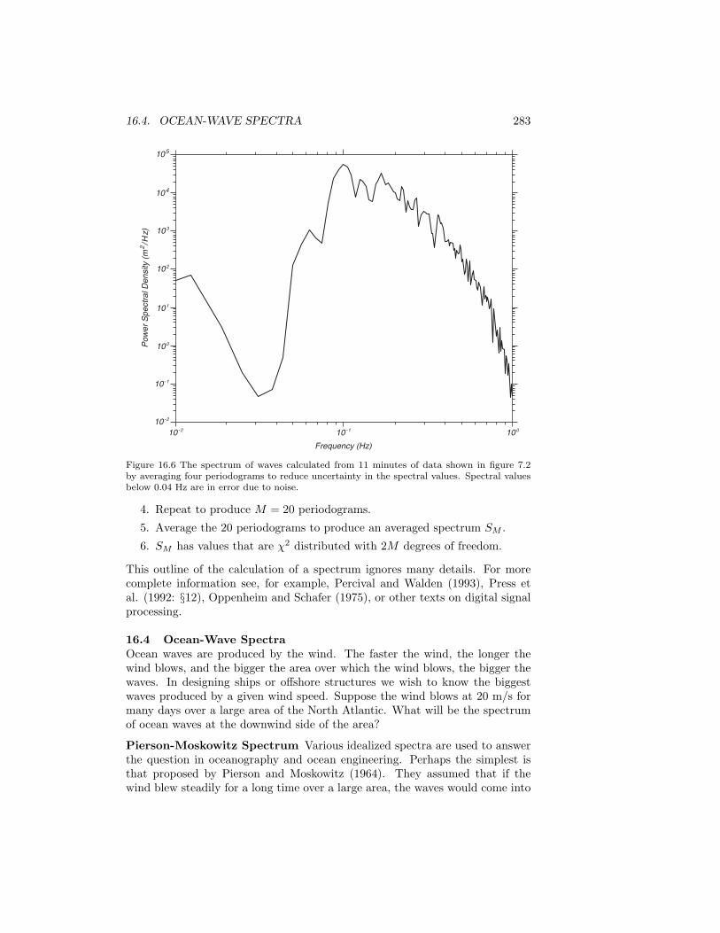
16.4. OCEAN-WAVE SPECTRA 283
Pow
er S
pect
ral D
ensi
ty (
m2/H
z)
104
105
103
102
101
100
10-1
10-2
10-2 10-1 100
Frequency (Hz)
Figure 16.6 The spectrum of waves calculated from 11 minutes of data shown in figure 7.2by averaging four periodograms to reduce uncertainty in the spectral values. Spectral valuesbelow 0.04 Hz are in error due to noise.
4. Repeat to produce M = 20 periodograms.
5. Average the 20 periodograms to produce an averaged spectrum SM .
6. SM has values that are χ2 distributed with 2M degrees of freedom.
This outline of the calculation of a spectrum ignores many details. For morecomplete information see, for example, Percival and Walden (1993), Press etal. (1992: §12), Oppenheim and Schafer (1975), or other texts on digital signalprocessing.
16.4 Ocean-Wave SpectraOcean waves are produced by the wind. The faster the wind, the longer thewind blows, and the bigger the area over which the wind blows, the bigger thewaves. In designing ships or offshore structures we wish to know the biggestwaves produced by a given wind speed. Suppose the wind blows at 20 m/s formany days over a large area of the North Atlantic. What will be the spectrumof ocean waves at the downwind side of the area?
Pierson-Moskowitz Spectrum Various idealized spectra are used to answerthe question in oceanography and ocean engineering. Perhaps the simplest isthat proposed by Pierson and Moskowitz (1964). They assumed that if thewind blew steadily for a long time over a large area, the waves would come into

284 CHAPTER 16. OCEAN WAVES
0
10
30
50
60
80
90
110
100
70
40
20
0 0.05 0.10 0.15 0.20 0.25 0.30 0.35Frequency (Hz)
Wav
e S
pect
ral D
ensi
ty (
m2
/ Hz)
20.6 m/s
18 m/s
15.4 m/s
12.9 m/s10.3 m/s
Figure 16.7 Wave spectra of a fully developed sea for differentwind speeds according to Moskowitz (1964).
equilibrium with the wind. This is the concept of a fully developed sea. Here, a“long time” is roughly ten-thousand wave periods, and a “large area” is roughlyfive-thousand wave lengths on a side.
To obtain a spectrum of a fully developed sea, they used measurements ofwaves made by accelerometers on British weather ships in the North Atlantic.First, they selected wave data for times when the wind had blown steadily forlong times over large areas of the North Atlantic. Then they calculated the wavespectra for various wind speeds (figure 16.7), and they found that the function
S(ω) =αg2
ω5exp
[−β
(ω0
ω
)4]
(16.30)
was a good fit to the observed spectra, where ω = 2πf , f is the wave frequencyin Hertz, α = 8.1 × 10⁻³, β = 0.74 , ω0 = g/U19.5 and U19.5 is the wind speedat a height of 19.5 m above the sea surface, the height of the anemometers onthe weather ships used by Pierson and Moskowitz (1964).
For most airflow over the sea the atmospheric boundary layer has nearlyneutral stability, and
U19.5 ≈ 1.026 U10 (16.31)
assuming a drag coefficient of 1.3 × 10⁻³.

16.4. OCEAN-WAVE SPECTRA 285
The frequency of the peak of the Pierson-Moskowitz spectrum is calculatedby solving dS/dω = 0 for ωp, to obtain
ωp = 0.877 g/U19.5. (16.32)
The speed of waves at the peak is calculated from (16.7), which gives:
cp =g
ωp= 1.14 U19.5 ≈ 1.17 U10 (16.33)
Hence waves with frequency ωp travel 14% faster than the wind at a height of19.5 m or 17% faster than the wind at a height of 10 m. This poses a difficultproblem: How can the wind produce waves traveling faster than the wind? Wewill return to the problem after we discuss the jonswap spectrum and theinfluence of nonlinear interactions among wind-generated waves.
By integrating S(ω) over all ω we get the variance of surface elevation:
⟨ζ2
⟩=
∫ ∞
0
S(ω) dω = 2.74 × 10⁻³ (U19.5)4
g2(16.34)
Remembering that H1/3 = 4⟨ζ2
⟩1/2, the significant wave height is:
H1/3 = 0.21(U19.5)
2
g≈ 0.22
(U10)2
g(16.35)
Figure 16.8 gives significant wave heights and periods calculated from the Pierson-Moskowitz spectrum.
Period Height
0
5
10
15
20
0 5 10 15 20 25
Sig
nific
ant W
ave
Hei
ght (
m)
Per
iod
(s)
Wind Speed U10 (m/s)
0
5
10
15
20
Figure 16.8 Significant wave height and period at the peak of the spectrum of a fullydeveloped sea calculated from the Pierson-Moskowitz spectrum using (16.35 and 16.32).
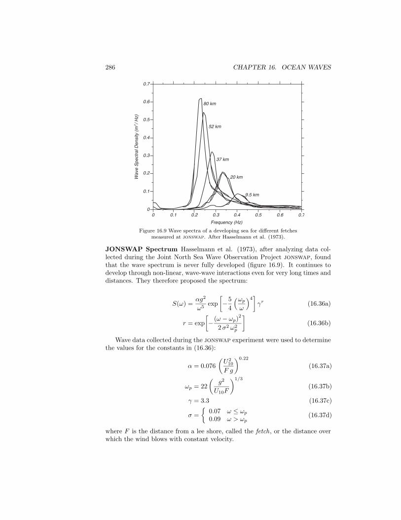
286 CHAPTER 16. OCEAN WAVES
80 km
52 km
37 km
20 km
9.5 km
0.1 0.2 0.3 0.4 0.5 0.6 0.7
0.1
0.2
0.3
0.4
0.5
0.6
0.7
Wav
e S
pect
ral D
ensi
ty (
m2/ H
z)
Frequency (Hz)
00
Figure 16.9 Wave spectra of a developing sea for different fetchesmeasured at jonswap. After Hasselmann et al. (1973).
JONSWAP Spectrum Hasselmann et al. (1973), after analyzing data col-lected during the Joint North Sea Wave Observation Project jonswap, foundthat the wave spectrum is never fully developed (figure 16.9). It continues todevelop through non-linear, wave-wave interactions even for very long times anddistances. They therefore proposed the spectrum:
S(ω) =αg2
ω5exp
[−5
4
(ωp
ω
)4]
γr (16.36a)
r = exp[− (ω − ωp)
2
2 σ2 ω2p
](16.36b)
Wave data collected during the jonswap experiment were used to determinethe values for the constants in (16.36):
α = 0.076(
U210
F g
)0.22
(16.37a)
ωp = 22(
g2
U10F
)1/3
(16.37b)
γ = 3.3 (16.37c)
σ =
0.07 ω ≤ ωp
0.09 ω > ωp(16.37d)
where F is the distance from a lee shore, called the fetch, or the distance overwhich the wind blows with constant velocity.

16.5. WAVE FORECASTING 287
The energy of the waves increases with fetch:
⟨ζ2
⟩= 1.67 × 10⁻⁷ (U10)
2
gF (16.38)
where F is fetch.The jonswap spectrum is similar to the Pierson-Moskowitz spectrum except
that waves continues to grow with distance (or time) as specified by the α term,and the peak in the spectrum is more pronounced, as specified by the γ term.The latter turns out to be particularly important because it leads to enhancednon-linear interactions and a spectrum that changes in time according to thetheory of Hasselmann (1966).
Generation of Waves by Wind We have seen in the last few paragraphsthat waves are related to the wind. We have, however, put off until now justhow they are generated by the wind. Suppose we begin with a mirror-smoothsea (Beaufort Number 0). What happens if the wind suddenly begins to blowsteadily at say 8 m/s? Three different physical processes begin:
1. The turbulence in the wind produces random pressure fluctuations at thesea surface, which produces small waves with wavelengths of a few cen-timeters (Phillips, 1957).
2. Next, the wind acts on the small waves, causing them to become larger.Wind blowing over the wave produces pressure differences along the waveprofile causing the wave to grow. The process is unstable because, as thewave gets bigger, the pressure differences get bigger, and the wave growsfaster. The instability causes the wave to grow exponentially (Miles, 1957).
3. Finally, the waves begin to interact among themselves to produce longerwaves (Hasselmann et al. 1973). The interaction transfers wave energyfrom short waves generated by Miles’ mechanism to waves with frequenciesslightly lower than the frequency of waves at the peak of the spectrum.Eventually, this leads to waves going faster than the wind, as noted byPierson and Moskowitz.
16.5 Wave ForecastingOur understanding of ocean waves, their spectra, their generation by the wind,and their interactions are now sufficiently well understood that the wave spec-trum can be forecast using winds calculated from numerical weather models. Ifwe observe some small ocean area, or some area just offshore, we can see wavesgenerated by the local wind, the wind sea, plus waves that were generated inother areas at other times and that have propagated into the area we are ob-serving, the swell. Forecasts of local wave conditions must include both sea andswell, hence wave forecasting is not a local problem. We saw, for example, thatwaves off California can be generated by storms more than 10,000 km away.
Various techniques have been used to forecast waves. The earliest attemptswere based on empirical relationships between wave height and wave lengthand wind speed, duration, and fetch. The development of the wave spectrum

288 CHAPTER 16. OCEAN WAVES
Global 1 x 1,25 grid 20 August 1998 00:00 UTCWind Speed in Knots
1
2
32
2
1
2
2
1
2
3
3
25
4
4
4
1
1
1
GM
Figure 16.10 Output of a third-generation wave forecast model produced by noaa’s OceanModeling Branch for 20 August 1998. Contours are significant wave height in meters, arrowsgive direction of waves at the peak of the wave spectrum, and barbs give wind speed in m/sand direction. From noaa Ocean Modeling Branch.
allowed evolution of individual wave components with frequency f travelling indirection θ of the directional wave spectrum ψ(f, θ) using
∂ψ0
∂t+ cg · ∇ψ0 = Si + Snl + Sd (16.39)
where ψ0 = ψ0(f, θ;x, t) varies in space (x) and time t, Si is input from the windgiven by the Phillips (1957) and Miles (1957) mechanisms, Snl is the transferamong wave components due to nonlinear interactions, and Sd is dissipation.
The third-generation wave-forecasting models now used by meteorologicalagencies throughout the world are based on integrations of (16.39) using manyindividual wave components (The swamp Group 1985; The wamdi Group, 1988;Komen et al, 1996). The forecasts follow individual components of the wavespectrum in space and time, allowing each component to grow or decay de-pending on local winds, and allowing wave components to interact according toHasselmann’s theory. Typically the sea is represented by 300 components: 25wavelengths going in 12 directions (30). To reduce computing time, the modelsuse a nested grid of points: the grid has a high density of points in storms andnear coasts and a low density in other regions. Typically, grid points in theopen ocean are 3 apart.

16.6. MEASUREMENT OF WAVES 289
Some recent experimental models take the wave-forecasting process one stepfurther by assimilating altimeter and scatterometer observations of wind speedand wave height into the model. Forecasts of waves using assimilated satel-lite data are available from the European Centre for Medium-Range WeatherForecasts.
noaa’s Ocean Modeling Branch at the National Centers for EnvironmentalPredictions also produces regional and global forecasts of waves. The Branch usea third-generation model based on the Cycle-4 wam model. It accommodatesever-changing ice edge, and it assimilates buoy and satellite altimeter wavedata. The model calculates directional frequency spectra in 12 directions and 25frequencies at 3-hour intervals up to 72 hours in advance. The lowest frequencyis 0.04177 Hz and higher frequencies are spaced logarithmically at incrementsof 0.1 times the lowest frequency. Wave spectral data are available on a 2.5×2.5 grid for deep-water points between 67.5S and 77.5N. The model is drivenusing 10-meter winds calculated from the lowest winds from the Centers weathermodel adjusted to a height of 10 meter by using a logarithmic profile (8.19). TheBranch is testing an improved forecast with 1× 1.25 resolution (figure 16.10).
16.6 Measurement of WavesBecause waves influence so many processes and operations at sea, many tech-niques have been invented for measuring waves. Here are a few of the morecommonly used. Stewart (1980) gives a more complete description of wavemeasurement techniques, including methods for measuring the directional dis-tribution of waves.
Sea State Estimated by Observers at Sea This is perhaps the most com-mon observation included in early tabulations of wave heights. These are thesignificant wave heights summarized in the U.S. Navy’s Marine ClimatologicalAtlas and other such reports printed before the age of satellites.
Accelerometer Mounted on Meteorological or Other Buoy This is aless common measurement, although it is often used for measuring waves dur-ing short experiments at sea. For example, accelerometers on weather shipsmeasured wave height used by Pierson & Moskowitz and the waves shown infigure 16.2. The most accurate measurements are made using an accelerometerstabilized by a gyro so the axis of the accelerometer is always vertical.
Double integration of vertical acceleration gives displacement. The doubleintegration, however, amplifies low-frequency noise, leading to the low frequencysignals seen in figures 16.4 and 16.5. In addition, the buoy’s heave is not sensitiveto wavelengths less than the buoy’s diameter, and buoys measure only waveshaving wavelengths greater than the diameter of the buoy. Overall, carefulmeasurements are accurate to ± 10% or better.
Wave Gages Gauges may be mounted on platforms or on the sea floor inshallow water. Many different types of sensors are used to measure the heightof the wave or subsurface pressure which is related to wave height. Sound,infrared beams, and radio waves can be used to determine the distance from

290 CHAPTER 16. OCEAN WAVES
0.56m SHW
1.94m SWH
-15 -10 -5 0 5 10 15 20
Time (ns)
Rec
eive
d po
wer
Figure 16.11 Shape of radio pulse received by the Seasat altimeter, showing the influenceof ocean waves. The shape of the pulse is used to calculate significant wave height. AfterStewart (1985: 264).
the sensor to the sea surface provided the sensor can be mounted on a stableplatform that does not interfere with the waves. Pressure gauges described in§6.8 can be used to measure the depth from the sea surface to the gauge. Arraysof bottom-mounted pressure gauges are useful for determining wave directions.Thus arrays are widely used just offshore of the surf zone to determine offshorewave directions.
Pressure gauge must be located within a quarter of a wavelength of thesurface because wave-induced pressure fluctuations decrease exponentially withdepth. Thus, both gauges and pressure sensors are restricted to shallow water orto large platforms on the continental shelf. Again, accuracy is ± 10% or better.
Satellite Altimeters The satellite altimeters used to measure surface geo-strophic currents also measure wave height. Altimeters were flown on Seasat in1978, Geosat from 1985 to 1988, ers–1 &2 from 1991, Topex/Poseidon from1992, and Jason from 2001. Altimeter data have been used to produce monthlymean maps of wave heights and the variability of wave energy density in timeand space. The next step, just begun, is to use altimeter observation with waveforecasting programs, to increase the accuracy of wave forecasts.
The altimeter technique works as follows. Radio pulse from a satellite al-timeter reflect first from the wave crests, later from the wave troughs. Thereflection stretches the altimeter pulse in time, and the stretching is measuredand used to calculate wave height (figure 16.11). Accuracy is ±10%.
Synthetic Aperture Radars on Satellites These radars map the radar re-flectivity of the sea surface with spatial resolution of 6–25 m. Maps of reflectivityoften show wave-like features related to the real waves on the sea surface. I say‘wave-like’ because there is not an exact one-to-one relationship between waveheight and image density. Some waves are clearly mapped, others less so. Themaps, however, can be used to obtain additional information about waves, espe-

16.7. IMPORTANT CONCEPTS 291
cially the spatial distribution of wave directions in shallow water (Vesecky andStewart, 1982). Because the directional information can be calculated directlyfrom the radar data without the need to calculate an image (Hasselmann, 1991),data from radars and altimeters on ers–1 & 2 are being used to determine if theradar and altimeter observations can be used directly in wave forecast programs.
16.7 Important Concepts1. Wavelength and frequency of waves are related through the dispersion
relation.
2. The velocity of a wave phase can differ from the velocity at which waveenergy propagates.
3. Waves in deep water are dispersive, longer wavelengths travel faster thanshorter wavelengths. Waves in shallow water are not dispersive.
4. The dispersion of ocean waves has been accurately measured, and obser-vations of dispersed waves can be used to track distant storms.
5. The shape of the sea surface results from a linear superposition of waves ofall possible wavelengths or frequencies travelling in all possible directions.
6. The spectrum gives the contributions by wavelength or frequency to thevariance of surface displacement.
7. Wave energy is proportional to variance of surface displacement.
8. Digital spectra are band limited, and they contain no information aboutwaves with frequencies higher than the Nyquist frequency.
9. Waves are generated by wind. Strong winds of long duration generate thelargest waves.
10. Various idealized forms of the wave spectrum generated by steady, homo-geneous winds have been proposed. Two important ones are the Pierson-Moskowitz and jonswap spectra.
11. Observations by mariners on ships and by satellite altimeters have beenused to make global maps of wave height. Wave gauges are used on plat-forms in shallow water and on the continental shelf to measure waves.Bottom-mounted pressure gauges are used to measure waves just offshoreof beaches. And synthetic-aperture radars are used to obtain informationabout wave directions.

292 CHAPTER 16. OCEAN WAVES

Chapter 17
Coastal Processes and Tides
In the last chapter I described waves on the sea surface. Now we can considerseveral special and important cases: the transformation of waves as they comeashore and break; the currents and edge waves generated by the interactionof waves with coasts; tsunamis; storm surges; and tides, especially tides alongcoasts.
17.1 Shoaling Waves and Coastal ProcessesWave phase and group velocities are a function of depth when the depth is lessthan about one-quarter wavelength in deep water. Wave period and frequencyare invariant (don’t change as the wave comes ashore); and this is used tocompute the properties of shoaling waves. Wave height increases as wave groupvelocity slows. Wave length decreases. Waves change direction due to refraction.Finally, waves break if the water is sufficiently shallow; and broken waves pourwater into the surf zone, creating long-shore and rip currents.
Shoaling Waves The dispersion relation (16.3) is used to calculate wave prop-erties as the waves propagate from deep water offshore to shallow water justoutside the surf zone. Because ω is constant, (16.3) leads to:
L
L0=
c
c0=
sinα
sinα0= tanh
2πd
L(17.1)
where
L0 =gT 2
2π, c0 =
gT
2π(17.2)
and L is wave length, c is phase velocity, α is the angle of the crest relativeto contours of constant depth, and d is water depth. The subscript 0 indicatesvalues in deep water.
The quantity d/L is calculated from the solution of
d
L0=
d
Ltanh
2πd
L(17.3)
293

294 CHAPTER 17. COASTAL PROCESSES AND TIDES
1.0
2.0
0.2
0.5
0.1
0.01 0.050.02 0.1 0.50.2 1.0
()
CG
C0
d L, t
anh
2π
dL
C C0
,L L 0
,si
n α
sin
α0
H H0
,,
d / L
)
( tanh
2πdL
CC0
,LL0
,sin α
sin α0 CG / C0
d / L0
CG / C
H / H0
deepshallow
Figure 17.1 Properties of waves in intermediate depths between deep and shallow water. d =depth, L = wavelength, C = phase velocity, Cg = group velocity, α = angle of crests relativeto contours of constant depth, H = wave height. Subscript 0 refers to properties in deepwater. From values in Wiegel (1964: A1).
using an iterative technique, or from figure 17.1, or from Wiegel (1964: A1).Because wave velocity is a function of depth in shallow water, variations
in offshore water depth can focus or defocus wave energy reaching the shore.Consider the simple case of waves with deep-water crests almost parallel to a
Beachdeposit
Headland
Headland
Wavefronts
Water depth (m)
Orthogonallines
Bay
80
60
40
20
Figure 17.2 Subsea features, such as submarine canyons and ridges, offshore of coasts cangreatly influence the height of breakers inshore of the features. After Thurman (1985: 229).

17.1. SHOALING WAVES AND COASTAL PROCESSES 295
1 2 3 4
(c) Surging breaker
(b) Plunging breaker
(a) Spilling breaker
1 2 3 4
1 2 3 4
Spillingbreaker
Plungingbreaker
Surging
0.06
0.07
0.05
0.04
0.03
0.02
0.01
00 0.02 0.04 0.06 0.08 0.10 0.12
Beach slope tanβ
Dee
pwat
er w
ave
stee
pnes
s H
o/Lo
Figure 17.3 Left: Classification of breaking waves as a function of beach steepness and wavesteepness offshore. Right: Sketch of types of breaking waves. After Horikawa (1988: 79, 81).
straight beach with two ridges each extending seaward from a headland (figure17.2). Wave group velocity is faster in the deeper water between the ridges, andthe wave crests become progressively deformed as the wave propagates towardthe beach. Wave energy, which propagates perpendicular to wave crests, isrefracted out of the region between the headland. As a result, wave energy isfocused into the headlands, and breakers there are much larger than breakers inthe bay. The difference in wave height can be surprisingly large. On a calm day,breakers can be knee high shoreward of a submarine canyon at La Jolla Shores,California, just south of the Scripps Institution of Oceanography. At the sametime, waves just north of the canyon can be high enough to attract surfers.
Breaking Waves As waves move into shallow water, the group velocity be-comes small, wave energy per square meter of sea surface increases, and non-linear terms in the wave equations become important. These processes causewaves to steepen, with short steep crests and broad shallow troughs. Whenwave slope at the crest becomes sufficiently steep, the wave breaks (figure 17.3Left). The shape of the breaking wave depends on the slope of the bottom, andthe steepness of waves offshore (figure 17.3 Right).
1. Steep waves tend to lose energy slowly as the waves moves into shallowerwater through water spilling down the front of the wave. These are spillingbreakers.
2. Less steep waves on steep beaches tend to steepen so quickly that thecrest of the wave moves much faster than the trough, and the crest, racingahead of the trough, plunges into the trough (figure 17.4).
3. If the beach is sufficiently steep, the wave can surge up the face of thebeach without breaking in the sense that white water is formed. Or if itis formed, it is at the leading edge of the water as it surges up the beach.An extreme example would be a wave incident on a vertical breakwater.

296 CHAPTER 17. COASTAL PROCESSES AND TIDES
Figure 17.4 Steep, plunging breakers are the archetypical breaker. The edgeof such breakers are ideal for surfing. From photo by Jeff Devine.
Wave-Driven Currents Waves break in a narrow band of shallow water alongthe beach, the surf zone. After breaking, waves continues as a near-vertical wallof turbulent water called a bore which carries water to the beach. At first, thebore surges up the beach, then retreats. The water carried by the bore is leftin the shallow waters inside the breaker zone.
Water dumped inside the breaker zone must return offshore. It does this byfirst moving parallel to the beach as an along-shore current . Then it turns andflows offshore perpendicular to the beach in a narrow, swift rip current . Therips are usually spaced hundreds of meters apart (figure 17.5). Usually there isa band of deeper water between the breaker zone and the beach, and the long-shore current runs in this channel. The strength of a rip current depends on the
Breaker Zone
Beach
Longshore Current
Rip
Cur
rent
Rip
Cur
rent
Coastal Current
Figure 17.5 Sketch of rip currents generated by water carried to the beach by breaking waves.

17.2. TSUNAMIS 297
height and frequency of breaking waves and the strength of the onshore wind.Rips are a danger to unwary swimmers, especially poor swimmers bobbing alongin the waves inside the breaker zone. They are carried along by the along-shorecurrent until they are suddenly carried out to sea by the rip. Swimming againstthe rip is futile, but swimmers can escape by swimming parallel to the beach.
Edge waves are produced by the variability of wave energy reaching shore.Waves tend to come in groups, especially when waves come from distant storms.For several minutes breakers may be smaller than average, then a few very largewaves will break. The minute-to-minute variation in the height of breakersproduces low-frequency variability in the along-shore current. This, in turn,drives a low-frequency wave attached to the beach, an edge wave. The waveshave periods of a few minutes, a long-shore wave length of around a kilometer,and an amplitude that decays exponentially offshore (figure 17.6).
z
x
y (north)
Figure 17.6 Computer-assisted sketch of an edge wave. Such waves exist in the breakerzone near the beach and on the continental shelf. After Cutchin and Smith (1973).
17.2 TsunamisTsunamis are low-frequency ocean waves generated by submarine earthquakes.The sudden motion of sea floor over distances of a hundred or more kilometersgenerates waves with periods of around 12 minutes (figure 17.7). A quick cal-culation shows that such waves must be shallow-water waves, propagating ata speed of 180 m/s and having a wavelength of 130 km in water 3.6 km deep(figure 17.8). The waves are not noticeable at sea, but after slowing on approachto the coast, and after refraction by subsea features, they can come ashore andsurge to heights ten or more meters above sea level. In an extreme example,the Alaskan tsunami on 1 April 1946 destroyed the Scotch Cap lighthouse 31 mabove sea level.
Shepard (1963, Chapter 4) summarized the influence of tsunamis based onhis studies in the Pacific.
1. Tsunamis appear to be produced by movement (an earthquake) along alinear fault.
2. Tsunamis can travel thousands of kilometers and still do serious damage.

298 CHAPTER 17. COASTAL PROCESSES AND TIDES
3:30
4:00
4:30
5:00
5:30
6:00
6:30
7:00
3:00
2:30
4000
2:00AM
KEYOrthogonalsWave Fronts 2:30A.M.Submarine Contours: m
550037001800
A L E U T I A NI S L A
ND
S
ALASKA
N O R T H
P A C I F I C
O C E A N
H A W A I I A NI S L A
ND
S20o
40o
45o
50o
55o
35o
30o
25o
-160o-170o -165o -155o -150o-175o
20'
22o0'
10'
50'
30' 20' 10'40'50'-160o0'
910
6:26
6:24
6:22
6:20
6:286:28
3700
2700
1800
910
550
1800
2700
180
2700
1800
1800
2700
WAIMEA
14
12m
5.22.4
4.6 2.4
7.6
4.6
8.5
3.7
7.3
3.76.1
1412
2.1
05:00
Approximate Time (hrs)
08:0006:00 07:00
1.0
0
0.8
0.4
Hei
ght (
m)
Waimeagauge
Figure 17.7 Left Hourly positions of leading edge of tsunami generated by the largeearthquake in the Aleutian Trench on April 1, 1946 at 1:59 AM Hawaiian time (12:59 GMT).Right: top Sealevel recorded by a river gauge in the estuary of the Waimea River. Right:lower Map of Kauai showing the heights reached by the water (in meters above lower lowwater) during the tsunami, wave fronts, orthogonals, and submarine contours. Times refer tothe computed arrival time of the first wave. After Shepard, MacDonald, and Cox (1950).
3. The first wave of a tsunami is not likely to be the biggest.4. Wave amplitudes are relatively large shoreward of submarine ridges. They
are relatively low shoreward of submarine valleys, provided the featuresextend into deep water.
5. Wave amplitudes are decreased by the presence of coral reefs borderingthe coast.
6. Some bays have a funneling effect, but long estuaries attenuate waves.7. Waves can bend around circular islands without great loss of energy, but
they are considerably smaller on the backsides of elongated, angular is-lands.
17.3 Storm SurgesStorm winds blowing over shallow, continental shelves pile water against thecoast. The increase in sea level is known as a storm surge. Several processes

17.3. STORM SURGES 299
Figure 17.8 Tsunami waves four hours after the great M9 Cascadia earthquake off the coast ofWashington on 26 January 1700 calculated by a finite-element, numerical model. Maximumopen-ocean wave height, about one meter, is north of Hawaii. After Satake et al. (1996).
are important:1. Ekman transport by winds parallel to the coast transports water toward
the coast causing a rise in sea level.2. Winds blowing toward the coast push water directly toward the coast.3. Wave run-up and other wave interactions transport water toward the coast
adding to the first two processes.4. Edge waves generated by the wind travel along the coast.5. The low pressure inside the storm raises sea level by one centimeter for
each millibar decrease in pressure through the inverted-barometer effect.6. Finally, the storm surge adds to the tides, and high tides can change a
relative weak surge into a much more dangerous one.
See Jelesnianski (1967, 1970) and §15.5 for a description of storm-surge modelssplash and Sea, Lake, and Overland Surges from Hurricanes slosh used bythe National Hurricane Center and §15.5.
To a crude first approximation, wind blowing over shallow water causes aslope in the sea surface proportional to wind stress.
∂ζ
∂x=
τ0
ρgH(17.4)
where ζ is sea level, x is horizontal distance, H is water depth, T0 is wind stressat the sea surface, ρ is water density; and g is gravitational acceleration.
If x = 100 km, U = 40 m/s, and H = 20 m, values typical of a hurricaneoffshore of the Texas Gulf Coast, then T = 2.7 Pa, and ζ = 1.3 m at the shore.Figure 17.9 shows the frequency of surges at the Netherlands and a graphicalmethod for estimating the probability of extreme events using the probabilityof weaker events.

300 CHAPTER 17. COASTAL PROCESSES AND TIDES
19531894
19161906
1928
1904
Mean High Water
103 102 10 1 10-1 10-2 10-3 10-4
0
1
2
3
4
5
Sto
rm S
urge
(m
)
Frequency per year
Figure 17.9 Probability (per year) density distribution of vertical height of storm surges inthe Hook of Holland in the Netherlands. The distribution function is Rayleigh, and theprobability of large surges is estimated by extrapolating the observed frequency of smaller,more common surges. After Wiegel (1964: 113).
17.4 Theory of Ocean TidesTides have been so important for commerce and science for so many thousandsof years that tides have entered our everyday language: time and tide wait forno one, the ebb and flow of events, a high-water mark, and turn the tide of battle.
1. Tides produce strong currents in many parts of the ocean. Tidal currentscan have speeds of up to 5 m/s in coastal waters, impeding navigation andmixing coastal waters.
2. Tidal currents generate internal waves over seamounts, continental slopes,and mid-ocean ridges. The waves dissipate tidal energy. Breaking internalwaves and tidal currents are a major force driving oceanic mixing.
3. Tidal currents can suspend bottom sediments, even in the deep ocean.
4. Earth’s crust is elastic. It bends under the influence of the tidal potential.It also bends under the weight of oceanic tides. As a result, the sea floor,and the continents move up and down by about 10 cm in response tothe tides. The deformation of the solid earth influence almost all precisegeodetic measurements.
5. Oceanic tides lag behind the tide-generating potential. This producesforces that transfer angular momentum between earth and the tide produc-ing body, especially the moon. As a result of tidal forces, earth’s rotationabout it’s axis slows, increasing the length of day; the rotation of the moonabout earth slows, causing the moon to move slowly away from earth; and

17.4. THEORY OF OCEAN TIDES 301
moon’s rotation about it’s axis slows, causing the moon to keep the sameside facing earth as the moon rotates about earth.
6. Tides influence the orbits of satellites. Accurate knowledge of tides isneeded for computing the orbit of altimetric satellites and for correctingaltimeter measurements of oceanic topography.
7. Tidal forces on other planets and stars are important for understandingmany aspects of solar-system dynamics and even galactic dynamics. Forexample, the rotation rate of Mercury, Venus, and Io result from tidalforces.
Mariners have known for at least four thousand years that tides are relatedto the phase of the moon. The exact relationship, however, is hidden behindmany complicating factors, and some of the greatest scientific minds of thelast four centuries worked to understand, calculate, and predict tides. Galileo,Descartes, Kepler, Newton, Euler, Bernoulli, Kant, Laplace, Airy, Lord Kelvin,Jeffreys, Munk and many others contributed. Some of the first computers weredeveloped to compute and predict tides. Ferrel built a tide-predicting machinein 1880 that was used by the U.S. Coast and Geodetic Survey to predict nineteentidal constituents. In 1901, Harris extended the capacity to 37 constituents.
Despite all this work important questions remained: What is the amplitudeand phase of the tides at any place on the ocean or along the coast? What isthe speed and direction of tidal currents? What is the shape of the tides onthe ocean? Where is tidal energy dissipated? Finding answers to these simplequestions is difficult, and the first, accurate, global maps of deep-sea tides wereonly published in 1994 (LeProvost et al. 1994). The problem is hard becausethe tides are a self-gravitating, near-resonant, sloshing of water in a rotating,elastic, ocean basin with ridges, mountains, and submarine basins.
Predicting tides along coasts and at ports is much simpler. Data from a tidegauge plus the theory of tidal forcing gives an accurate description of tides nearthe tide gauge.
Tidal Potential Tides are calculated from the hydrodynamic equations for aself-gravitating ocean on a rotating, elastic earth. The driving force is the smallchange in gravity due to motion of the moon and sun relative to earth.
The small variations in gravity arise from two separate mechanisms. To seehow they work, consider the rotation of moon about earth.
1. Moon and earth rotate about the center of mass of the earth-moon system.This gives rise to a centripetal acceleration at earth’s surface that driveswater away from the center of mass and toward the side of earth oppositemoon.
2. At the same time, mutual gravitational attraction of mass on earth andthe moon causes water to be attracted toward the moon.
If earth were an ocean planet with no land, and if the ocean were very deep, thetwo processes would produce a pair of bulges of water on earth, one on the sidefacing the moon, one on the side away from the moon. A clear derivation of

302 CHAPTER 17. COASTAL PROCESSES AND TIDES
the forces is given by Pugh (1987) and by Dietrich, Kalle, Krauss, and Siedler(1980). Here I follow the discussion in Pugh (1987: §3.2).
Celestialbody
A
P
R
Earth
O
rr1
ϕ
Figure 17.10 Sketch of coordinates for determining the tide-generating potential.
To calculate the amplitude and phase of the tide on an ocean planet, webegin by calculating the tide-generating potential. This is much simpler thancalculating the forces. The tide-generating potential at earth’s surface is dueto the earth-moon system rotating about a common center of mass. Ignoringfor now earth’s rotation, the rotation of moon about earth produces a potentialVM at any point on earth’s surface
VM = −γM
r1(17.5)
where the geometry is sketched in figure 17.10, γ is the gravitational constant,and M is moon’s mass. From the triangle OPA in the figure,
r21 = r2 + R2 − 2rR cos ϕ (17.6)
Using this in (17.5) gives
VM = −γM
R
1 − 2
( r
R
)cos ϕ +
( r
R
)1/2−1/2
(17.7)
r/R ≈ 1/60, and (17.7) may be expanded in powers of r/R using Legendrepolynomials (Whittaker and Watson, 1963: §15.1):
VM = −γM
R
1 +
( r
R
)cos ϕ +
( r
R
)2(
12
)(3 cos2 ϕ − 1) + · · ·
(17.8)
The tidal forces are calculated from the gradient of the potential, so the firstterm in (17.8) produces no force. The second term produces a constant forceparallel to OA. This force keeps earth in orbit about the center of mass of theearth-moon system. The third term produces the tides, assuming the higher-order terms can be ignored. The tide-generating potential is therefore:
V = −γMr2
2R3(3 cos2 ϕ − 1) (17.9)
The tide-generating force can be decomposed into components perpendicularP and parallel H to the sea surface. Tides are produced by the horizontalcomponent. “The vertical component is balanced by pressure on the sea bed,

17.4. THEORY OF OCEAN TIDES 303
Z
30o
-30o
0o
60o
Figure 17.11 The horizontal component of the tidal force on earth when thetide-generating body is above the Equator at Z. After Dietrich et al. (1980: 413).
but the ratio of the horizontal force per unit mass to vertical gravity has to bebalanced by an opposing slope of the sea surface, as well as by possible changesin current momentum” (Cartwright, 1999: 39, 45). The horizontal component,shown in figure 17.11, is:
H = −1r
∂V
∂ϕ=
2G
rsin 2ϕ (17.10)
where
G =34γM
(r2
R3
)(17.11)
The tidal potential is symmetric about the earth-moon line, and it producessymmetric bulges.
If we allow our ocean-covered earth to rotate, an observer in space seesthe two bulges fixed relative to the earth-moon line as earth rotates. To anobserver on earth, the two tidal bulges seems to rotate around earth becausemoon appears to move around the sky at nearly one cycle per day. Moonproduces high tides every 12 hours and 25.23 minutes on the equator if themoon is above the equator. Notice that high tides are not exactly twice per daybecause the moon is also rotating around earth. Of course, the moon is abovethe equator only twice per lunar month, and this complicates our simple pictureof the tides on an ideal ocean-covered earth. Furthermore, moon’s distance fromearth R varies because moon’s orbit is elliptical and because the elliptical orbitis not fixed.
Clearly, the calculation of tides is getting more complicated than we mighthave thought. Before continuing on, we note that the solar tidal forces arederived in a similar way. The relative importance of the sun and moon arenearly the same. Although the sun is much more massive than moon, it is much

304 CHAPTER 17. COASTAL PROCESSES AND TIDES
further away.
Gsun = GS =34γS
(r2
R3sun
)(17.12)
Gmoon = GM =34γM
(r2
R3moon
)(17.13)
GS
GM= 0.46051 (17.14)
where Rsun is the distance to the sun, S is the mass of the sun, Rmoon is thedistance to the moon, and M is the mass of the moon.
Coordinates of Sun and Moon Before we can proceed further we need toknow the position of moon and sun relative to earth. An accurate description ofthe positions in three dimensions is very difficult, and it involves learning arcaneterms and concepts from celestial mechanics. Here, I paraphrase a simplifieddescription from Pugh (1987). See also figure 4.1.
A natural reference system for an observer on earth is the equatorial systemdescribed at the start of Chapter 3. In this system, declinations δ of a celestialbody are measured north and south of a plane which cuts the earth’s equator.
Angular distances around the plane are measured relative to a pointon this celestial equator which is fixed with respect to the stars. Thepoint chosen for this system is the vernal equinox, also called the ‘FirstPoint of Aries’ . . . The angle measured eastward, between Aries and theequatorial intersection of the meridian through a celestial object is calledthe right ascension of the object. The declination and the right ascensiontogether define the position of the object on a celestial background . . .
[Another natural reference] system uses the plane of the earth’s revo-lution around the sun as a reference. The celestial extension of this plane,which is traced by the sun’s annual apparent movement, is called theecliptic. Conveniently, the point on this plane which is chosen for a zeroreference is also the vernal equinox, at which the sun crosses the equatorialplane from south to north around 21 March each year. Celestial objectsare located by their ecliptic latitude and ecliptic longitude. The anglebetween the two planes, of 23.45, is called the obliquity of the ecliptic. . . —Pugh (1987: 72).
Tidal Frequencies Now, let’s allow earth to spin about its polar axis. Thechanging potential at a fixed geographic coordinate on earth is:
cos ϕ = sinϕp sin δ + cos ϕp cos δ cos(τ1 − 180) (17.15)
where ϕp is latitude at which the tidal potential is calculated, δ is declinationof moon or sun north of the equator, and τ1 is the hour angle of moon or sun.The hour angle is the longitude where the imaginary plane containing the sunor moon and earth’s rotation axis crosses the Equator.
The period of the solar hour angle is a solar day of 24 hr 0 m. The periodof the lunar hour angle is a lunar day of 24 hr 50.47 m.

17.4. THEORY OF OCEAN TIDES 305
Earth’s axis of rotation is inclined 23.45 with respect to the plane of earth’sorbit about the sun. This defines the ecliptic, and the sun’s declination variesbetween δ = ±23.45 with a period of one solar year. The orientation of earth’srotation axis precesses with respect to the stars with a period of 26 000 years.The rotation of the ecliptic plane causes δ and the vernal equinox to changeslowly, and the movement called the precession of the equinoxes .
Earth’s orbit about the sun is elliptical, with the sun in one focus. That pointin the orbit where the distance between the sun and earth is a minimum is calledperigee. The orientation of the ellipse in the ecliptic plane changes slowlywith time, causing perigee to rotate with a period of 20 942 years. ThereforeRsun varies with this period.
Moon’s orbit is also elliptical, but a description of moon’s orbit is muchmore complicated than a description of earth’s orbit. Here are the basics. Themoon’s orbit lies in a plane inclined at a mean angle of 5.15 relative to theplane of the ecliptic. And lunar declination varies between δ = 23.45 ± 5.15
with a period of one tropical month of 27.32 solar days. The actual inclinationof moon’s orbit varies between 4.97, and 5.32.
The shape of moon’s orbit also varies. First, perigee rotates with a periodof 8.85 years. The eccentricity of the orbit has a mean value of 0.0549, andit varies between 0.044 and 0.067. Second, the plane of moon’s orbit rotatesaround earth’s axis of rotation with a period of 18.613 years. Both processescause variations in Rmoon.
Note that I am a little imprecise in defining the position of the sun andmoon. Lang (1980: § 5.1.2) gives much more precise definitions.
Substituting (17.15) into (17.9) gives:
V =γMr2
R3
14
[(3 sin2 ϕp − 1
) (3 sin2 δ − 1
)+ 3 sin 2ϕp sin 2δ cos τ1
+ 3 cos2 ϕp cos2 δ cos 2τ1
](17.16)
Equation (17.16) separates the period of the lunar tidal potential into threeterms with periods near 14 days, 24 hours, and 12 hours. Similarly the solarpotential has periods near 180 days, 24 hours, and 12 hours. Thus there arethree distinct groups of tidal frequencies: twice-daily, daily, and long period,having different latitudinal factors sin2 θ, sin 2θ, and (1− 3 cos2 θ)/2, where θ isthe co-latitude (90 − ϕ).
Doodson (1922) expanded (17.16) in a Fourier series using the cleverly chosenfrequencies in table 17.1. Other choices of fundamental frequencies are possible,for example the local, mean, solar time can be used instead of the local, mean,lunar time. Doodson’s expansion, however, leads to an elegant decompositionof tidal constituents into groups with similar frequencies and spatial variability.
Using Doodson’s expansion, each constituent of the tide has a frequency
f = n1f1 + n2f2 + n3f3 + n4f4 + n5f5 + n6f6 (17.17)

306 CHAPTER 17. COASTAL PROCESSES AND TIDES
Table 17.1 Fundamental Tidal Frequencies
Frequency Period Source/hour
f1 14.49205211 1 lunar day Local mean lunar timef2 0.54901653 1 month Moon’s mean longitudef3 0.04106864 1 year Sun’s mean longitudef4 0.00464184 8.847 years Longitude of moon’s perigeef5 -0.00220641 18.613 years Longitude of moon’s ascending nodef6 0.00000196 20,940 years Longitude of sun’s perigee
where the integers ni are the Doodson numbers. n1 = 1, 2, 3 and n2–n6 arebetween −5 and +5. To avoid negative numbers, Doodson added five to n2···6.Each tidal wave having a particular frequency given by its Doodson number iscalled a tidal constituent , sometimes called a partial tides. For example, theprincipal, twice-per-day, lunar tide has the number 255.555. Because the verylong-term modulation of the tides by the change in sun’s perigee is so small, thelast Doodson number n6 is usually ignored.
If the ocean surface is in equilibrium with the tidal potential, which meanswe ignore inertia and currents and assume no land, the largest tidal constituentswould have amplitudes given in table 17.2. Notice that tides with frequenciesnear one or two cycles per day are split into closely spaced lines with spacingseparated by a cycle per month. Each of these lines is further split into linesseparated by a cycle per year (figure 17.12). Furthermore, each of these linesis split into lines separated by a cycle per 8.8 yr, and so on. Clearly, there are
Table 17.2 Principal Tidal Constituents
EquilibriumTidal Amplitude† PeriodSpecies Name n1 n2 n3 n4 n5 (m) (hr)
Semidiurnal n1 = 2
Principal lunar M2 2 0 0 0 0 0.242334 12.4206Principal solar S2 2 2 -2 0 0 0.112841 12.0000Lunar elliptic N2 2 -1 0 1 0 0.046398 12.6584Lunisolar K2 2 2 0 0 0 0.030704 11.9673
Diurnal n1 = 1
Lunisolar K1 1 1 0 0 0 0.141565 23.9344Principal lunar O1 1 -1 0 0 0 0.100514 25.8194Principal solar P1 1 1 -2 0 0 0.046843 24.0659Elliptic lunar Q1 1 -2 0 1 0 0.019256 26.8684
Long Period n1 = 0
Fortnightly Mf 0 2 0 0 0 0.041742 327.85Monthly Mm 0 1 0 -1 0 0.022026 661.31Semiannual Ssa 0 0 2 0 0 0.019446 4383.05
†Amplitudes from Apel (1987)

17.4. THEORY OF OCEAN TIDES 307
Frequency (deg/hr)
3N2
ε2
2N2 µ2
N2
ν2
γ2
α2
M2
β2
δ2
λ2
L2
2T2
T2
S2
K2
R2
ζ2
η2
2T2
T2
S2
K2
R2
Am
plitu
de (
cm)
10 -2
10-1
100
101
102
26 27 28 29 30 31 32
Am
plitu
de (
cm)
29.80 29.85 29.90 29.95 30.00 30.05 30.10 30.15 30.20
Frequency (deg/hr)
10-2
10-1
100
101
102
Figure 17.12 Upper: Spectrum of equilibrium tides with frequencies near twice per day.The spectrum is split into groups separated by a cycle per month (0.55 deg/hr). Lower:Expanded spectrum of the S2 group, showing splitting at a cycle per year (0.04 deg/hr).The finest splitting in this figure is at a cycle per 8.847 years (0.0046 deg/hr). From RichardEanes, Center for Space Research, University of Texas.
very many possible tidal constituents.Why is the tide split into the many constituents shown in figure 17.12? To
answer the question, suppose moon’s elliptical orbit was in the equatorial planeof earth. Then δ = 0. From (17.16), the tidal potential on the equator, whereϕp = 0, is:
V =γMr2
R3
14
cos (4πf1) (17.18)
If the ellipticity of the orbit is small, R = R0(1+ε), and (17.18) is approximately
V = a(1 − 3ε) cos (4πf1) (17.19)
where a =(γMr2
)/
(4R3
)is a constant. ε varies with a period of 27.32 days,
and we can write ε = b cos(2πf2) where b is a small constant. With thesesimplifications, (17.19) can be written:
V = a cos (4πf1) − 3ab cos (2πf2) cos (4πf1) (17.20a)V = a cos (4πf1) − 3ab [cos 2π (2f1 − f2) + cos 2π (2f1 + f2)] (17.20b)

308 CHAPTER 17. COASTAL PROCESSES AND TIDES
which has a spectrum with three lines at 2f1 and 2f1 ± f2. Therefore, the slowmodulation of the amplitude of the tidal potential at two cycles per lunar daycauses the potential to be split into three frequencies. This is the way amplitudemodulated AM radio works. If we add in the the slow changes in the shape ofthe orbit, we get still more terms even in this very idealized case of a moon inan equatorial orbit.
If you are very observant, you will have noticed that the tidal spectrumin figure 17.12 does not look like the ocean-wave spectrum of ocean waves infigure 16.6. Ocean waves have all possible frequencies, and their spectrum iscontinuous. Tides have precise frequencies determined by the orbit of earth andmoon, and their spectrum is not continuous. It consists of discrete lines.
Doodson’s expansion included 399 constituents, of which 100 are long period,160 are daily, 115 are twice per day, and 14 are thrice per day. Most have verysmall amplitudes, and only the largest are included in table 17.2. The largesttides were named by Sir George Darwin (1911) and the names are included inthe table. Thus, for example, the principal, twice-per-day, lunar tide, which hasDoodson number 255.555, is the M2 tide, called the M-two tide.
17.5 Tidal PredictionIf tides in the ocean were in equilibrium with the tidal potential, tidal predictionwould be much easier. Unfortunately, tides are far from equilibrium. Theshallow-water wave which is the tide cannot move fast enough to keep up withsun and moon. On the equator, the tide would need to propagate around theworld in one day. This requires a wave speed of around 460 m/s, which isonly possible in an ocean 22 km deep. In addition, the continents interrupt thepropagation of the wave. How to proceed?
We can separate the problem of tidal prediction into two parts. The firstdeals with the prediction of tides in ports and shallow water where tides can bemeasured by tide gauges. The second deals with the prediction of tides in thedeep ocean where tides are measured by satellite altimeters.
Tidal Prediction for Ports and Shallow Water Two methods are used topredict future tides at a tide-gauge station using past observations of sea levelmeasured at the gauge.
The Harmonic Method This is the traditional method, and it is still widelyused. The method typically uses 19 years of data from a coastal tide gauge fromwhich the amplitude and phase of each tidal constituent (the tidal harmonics)in the tide-gage record are calculated. The frequencies used in the analysis arespecified in advance from the basic frequencies given in table 17.1.
Despite its simplicity, the technique had disadvantages compared with theresponse method described below.
1. More than 18.6 years of data are needed to resolve the modulation of thelunar tides.
2. Amplitude accuracy of 10−3 of the largest term require that at least 39frequencies be determined. Doodson found 400 frequencies were neededfor an amplitude accuracy of 10−4 of the largest term.

17.5. TIDAL PREDICTION 309
3. Non-tidal variability introduces large errors into the calculated amplitudesand phases of the weaker tidal constituents. The weaker tides have ampli-tudes smaller than variability at the same frequency due to other processessuch as wind set up and currents near the tide gauge.
4. At many ports, the tide is non-linear, and many more tidal constituents areimportant. For some ports, the number of frequencies is unmanageable.When tides propagate into very shallow water, especially river estuaries,they steepen and become non-linear. This generates harmonics of the orig-inal frequencies. In extreme cases, the incoming waves steepens so muchthe leading edge is nearly vertical, and the wave propagates as solitarywave. This is a tidal bore.
The Response Method This method, developed by Munk and Cartwright(1966), calculates the relationship between the observed tide at some point andthe tidal potential. The relationship is the spectral admittance between themajor tidal constituents and the tidal potential at each station. The admittanceis assumed to be a slowly varying function of frequency so that the admittanceof the major constituents can be used for determining the response at nearbyfrequencies. Future tides are calculated by multiplying the tidal potential bythe admittance function.
1. The technique requires only a few months of data.
2. The tidal potential is easily calculated, and a knowledge of the tidal fre-quencies is not needed.
3. The admittance is Z(f) = G(f)/H(f). G(f) and H(f) are the Fouriertransforms of the potential and the tide gage data, and f is frequency.
4. The admittance is inverse transformed to obtain the admittance as a func-tion of time.
5. The technique works only if the waves propagate as linear waves.
Tidal Prediction for Deep-Water Prediction of deep-ocean tides has beenmuch more difficult than prediction of shallow-water tides because tide gaugeswere seldom deployed in deep water. All this changed with the launch ofTopex/Poseidon. The satellite was placed into an orbit especially designed forobserving ocean tides (Parke et al. 1987), and the altimetric system was suf-ficiently accurate to measure many tidal constituents. Data from the satellitehave now been used to determine deep-ocean tides with an accuracy of ± 2 cm.For most practical purposes, the tides are now known accurately for most of theocean.
Several approaches have led to the new knowledge of deep-water tides usingaltimetry.
Prediction Using Hydrodynamic Theory Purely theoretical calculations oftides are not very accurate, especially because the dissipation of tidal energyis not well known. Nevertheless, theoretical calculations provide insight intoprocesses influencing ocean tides. Several processes must be considered:

310 CHAPTER 17. COASTAL PROCESSES AND TIDES
1. The tides in one ocean basin perturb earth’s gravitational field, and themass in the tidal bulge attracts water in other ocean basins. The self-gravitational attraction of the tides must be included.
2. The weight of the water in the tidal bulge is sufficiently great that itdeforms the sea floor. The earth deforms as an elastic solid, and thedeformation extends thousands of kilometers.
3. The ocean basins have a natural resonance close to the tidal frequencies.The tidal bulge is a shallow-water wave on a rotating ocean, and it propa-gates as a high tide rotating around the edge of the basin. Thus the tidesare a nearly resonant sloshing of water in the ocean basin. The actual tideheights in deep water can be higher than the equilibrium values noted intable 17.2.
4. Tides are dissipated by bottom friction especially in shallow seas, by theflow over seamounts and mid-ocean ridges, and by the generation of in-ternal waves over seamounts and at the edges of continental shelves. Ifthe tidal forcing stopped, the tides would continue sloshing in the oceanbasins for several days.
5. Because the tide is a shallow-water wave everywhere, its velocity dependson depth. Tides propagate more slowly over mid-ocean ridges and shallowseas. Hence, the distance between grid points in numerical models mustbe proportional to depth with very close spacing on continental shelves(LeProvost et al. 1994).
6. Internal waves generated by the tides produce a small signal at the seasurface near the tidal frequencies, but not phase-locked to the potential.The noise near the frequency of the tides causes the spectral cusps inthe spectrum of sea-surface elevation first seen by Munk and Cartwright(1966). The noise is due to deep-water, tidally generated, internal waves.
Altimetry Plus Response Method Several years of altimeter data from Topex/Poseidon have been used with the response method to calculate deep-sea tidesalmost everywhere equatorward of 66 (Ma et al. 1994). The altimeter measuredsea-surface heights in geocentric coordinates at each point along the subsatel-lite track every 9.97 days. The temporal sampling aliased the tides into longfrequencies, but the aliased periods are precisely known and the tides can berecovered (Parke et al. 1987). Because the tidal record is shorter than 8 years,the altimeter data are used with the response method to obtain predictions fora much longer time.
Recent solutions by ten different groups, have accuracy of ± 2.8 cm in deepwater (Andersen, Woodworth, and Flather, 1995). Work has begun to improveknowledge of tides in shallow water.
Maps produced by this method show the essential features of the deep-oceantides (figure 17.13). The tide consists of a crest that rotates counterclockwisearound the ocean basins in the northern hemisphere, and in the opposite di-rection in the southern hemisphere. Points of minimum amplitude are calledamphidromes. Highest tides tend to be along the coast.

17.5. TIDAL PREDICTION 311
60o 120o 180o -120o -60o 0o
-60o
-30o
0o
30o
60o
1010
10
10
1010
101010
20
20
20
20
20 20
20
2020
20
2020
20
20
20
20
20
20
20
20
20
20
30
30
30
30
30
30
30
30
30
30
30
30
30
30
30
30
30
30
40
40
40
40
40
4040
40
4040
40
40
40
50
50
50
50
50
50
50
50 50
50
60
60
60
60
70
70800
0
0
0
0
00
0
0
0
60
60
60
60
60
60
60
120
120
120
120
120
120
120
180
180
180180
180 180
240
240
240
240
300
300
300
300
300
300
M2
Figure 17.13 Global map of M2 tide calculated from Topex/Poseidon observations of theheight of the sea surface combined with the response method for extracting tidal information.Full lines are contours of constant tidal phase, contour interval is 30. Dashed lines are linesof constant amplitude, contour interval is 10 cm. From Richard Ray, nasa Goddard SpaceFlight Center.
Altimetry Plus Numerical Models Altimeter data can be used directly withnumerical models of the tides to calculate tides in all areas of the ocean from
deep water all the way to the coast. Thus the technique is especially usefulfor determining tides near coasts and over sea-floor features where the altimeterground track is too widely spaced to sample the tides well in space. Tide modelsuse finite-element grids similar to the one shown in figure 15.3. Recent numericalcalculations by (LeProvost et al. 1994; LeProvost, Bennett, and Cartwright,1995) give global tides with ± 2–3 cm accuracy and full spatial resolution.
Further improvements will lead to solutions at the ultimate limits of practicalaccuracy, which is about ± 1–2 cm. The limit is set by noise from internal waveswith tidal frequency, and the small, long-term variations of depth of the ocean.Changing heat content of the ocean produces changes in oceanic topography ofa few centimeters, and this changes ever so slightly the velocity of shallow-waterwaves.
Tidal Dissipation Tides dissipate 3.75 ± 0.08 TW of power (Kantha, 1998),of which 3.5 TW are dissipated in the ocean, and much smaller amounts inthe atmosphere and solid earth. The dissipation increases the length of dayby about 2.07 milliseconds per century, it causes the semimajor axis of moon’sorbit to increase by 3.86 cm/yr, and it mixes water masses in the ocean.
The calculations of dissipation from Topex/Poseidon observations of tidesare remarkably close to estimates from lunar-laser ranging, astronomical obser-vations, and ancient eclipse records. Our knowledge of the tides is now suffi-ciently good that we can begin to use the information to study mixing in theocean. Remember, mixing helps drive the abyssal circulation in the ocean asdiscussed in §13.2 (Munk and Wunsch, 1998). Who would have thought that an

312 CHAPTER 17. COASTAL PROCESSES AND TIDES
understanding of the influence of the ocean on climate would require accurateknowledge of tides?
17.6 Important Concepts1. Waves propagating into shallow water are refracted by features of the
sea floor, and they eventually break on the beach. Breaking waves drivenear-shore currents including long-shore currents, rip currents, and edgewaves.
2. Storm surges are driven by strong winds in storms close to shore. Theamplitude of the surge is a function of wind speed, the slope of the seafloor,and the propagation of the storm.
3. Tides are important for navigation; they influence accurate geodetic mea-surements; and they change the orbits and rotation of planets, moons, andstars in galaxies.
4. Tides are produced by a combination of time-varying gravitational poten-tial of the moon and sun and the centrifugal forces generated as earthrotates about the common center of mass of the earth-moon-sun system.
5. Tides have six fundamental frequencies. The tide is the superposition ofhundreds of tidal constituents, each having a frequency that is the sumand difference of five fundamental frequencies.
6. Shallow water tides are predicted using tide measurements made in portsand other locations along the coast. Tidal records of just a few monthsduration can be used to predict tides many years into the future.
7. Tides in deep water are calculated from altimetric measurements, espe-cially Topex/Poseidon measurements. As a result, deep water tides areknown almost everywhere with an accuracy approaching ±2 cm.
8. The dissipation of tidal energy in the ocean transfers angular momentumfrom moon to earth, causing the day to become longer.
9. Tidal dissipation mixes water masses, and it is a major driver of the deep,meridional-overturning circulation. Tides, abyssal circulation, and climateare closely linked.

References
Alley R.B. 2000. Ice-core evidence of abrupt climate change. Proceedings of NationalAcademy of Sciences 97 (4): 1331–1334.
Apel J.R. 1987. Principles of Ocean Physics. New York: Academic Press.
Andersen O.B., P.L. Woodworth, and R.A. Flather. 1995. Intercomparison of recent oceantide models. J. Geophysical Research 100 (C12): 25,262–25,282.
Arthur R.S. 1960. A review of the calculation of ocean currents at the equator. Deep-SeaResearch 6 (4): 287–297.
Atlas R., R.N. Hoffman, and S.C. Bloom. 1993. Surface wind velocity over the oceans. InAtlas of satellite observations related to global change. Edited by R. J. Gurney, J. L.Foster and C. L. Parkinson. 129–140. Cambridge: University Press.
Atlas R., R.N. Hoffman, S.C. Bloom, J.C. Jusem, and J. Ardizzone. 1996. A multiyearglobal surface wind velocity dataset using SSM/I wind observations. Bulletin of theAmerican Meteorological Society 77 (5): 869–882.
Baker D.J. 1981. Ocean instruments and experiment design. In Evolution of PhysicalOceanography: Scientific Surveys in Honor of Henry Stommel. Edited by B. A. Warrenand C. Wunsch. 396–433. Cambridge: MIT Press.
Barnett T.P., M. Latif, N.E. Graham, M. Flugel, S. Pazan, and W. White. 1993. ensoand enso-related predictability. Part I: Prediction of equatorial Pacific sea surfacetemperature in a hybrid coupled ocean-atmosphere model. Journal of Climate 6: 1545–1566.
Barnier B., L. Siefridt, and P. Marchesiello. 1995. Thermal forcing for a global oceancirculation model using a three-year climatology of ecmwf analyses. Journal of MarineSystems 6: 393–380.
Batchelor G.K. 1967. An Introduction to Fluid Dynamics. Cambridge: The UniversityPress.
Baumgartner A., and E. Reichel. 1975. The World Water Balance. New York: Elsevier.
Beardsley R.C., A.G. Enriquez, C.A. Friehe, and C.A. Alessi. 1997. Intercomparison ofaircraft and buoy measurements of wind speed and wind stress during smile. Journalof Atmospheric and Oceanic Technology 14: 969–977.
Behringer D. W., M. Ji and A. Leetmaa. 1998. An improved coupled model for ENSO pre-diction and implications for ocean initialization: Part 1: The ocean data assimilation.Monthly Weather Review 126(4): 1013–1021.
Bennett A.F. 1992. Inverse Methods in Physical Oceanography. Cambridge: The UniversityPress.
Berlinski , D. 1996. The end of materialist science. Forbes ASAP (December 2, 1996):146–160.
Binder R.C. 1949. Fluid Mechanics. Second ed. New York: Prentice–Hall, Inc.
313

314 REFERENCES
Bjerknes J. 1966. The possible response of the atmospheric Hadley circulation to equatorialanomalies of ocean temperature. Tellus 4: 820-929.
Bjerknes J. 1972. Large-scale atmospheric response to the 1964–65 Pacific equatorial warm-ing. Journal of Physical Oceanography 2 (3): 212–217.
Bjerknes V. and J.W. Sandstrom. 1910. Dynamic Meteorology and Hydrography, Part I.Statics. Carnegie Institution of Washington DC, Publication No. 88.
Blumberg A.F., and G.L. Mellor. 1987. A description of a three-dimensional ocean circu-lation model. In: Three-Dimensional Coastal Ocean Models. Edited by N. S. Heaps.1–16. Washington, DC: American Geophysical Union.
Bond G., H. Heinrich, W. Broecker, L. Labeyrie, J. McManus, J. Andrews, S. Huon, R.Jantschik, S. Clasen, C. Simet, K. Tedesco, M. Klas, G. Bonani, and S. Ivy. 1992.Evidence for massive discharges of icebergs into the North Atlantic ocean during thelast glacial period. Nature 360, 245–.
Born G. H., Tapley, B. D., Ries, J. C., and Stewart, R. H. 1986. Accurate Measurementof Mean Sea Level Changes by Altimetric Satellites. Journal of Geophysical Research91(C10): 11,775–11,782.
Boville B.A., and P.R. Gent. 1998. The NCAR Climate System Model, Version One. Jour-nal of Climate 11 (6): 1115-1130.
Bowden K.F. 1962. Turbulence. In The Sea Volume 1. Edited by M. N. Hill. 802–825.New York: Interscience Publishers, John Wiley and Sons.
Bracewell R.N. 1986. The Fourier Transform and Its Applications. Second, revised ed.New York: McGraw-Hill Publishing Company.
Broecker W. S. 1987. Unpleasant surprises in the greenhouse? Nature 328: 123–126.
Broecker W.S. 1997. Thermohaline circulation, the Achilles heel of our climate system: Willman-made CO2 upset the current balance? Science 278 (5343): 1582–1588.
Bryan K. 1969. A numerical method for the study of the world ocean. J. ComputationalPhysics 4: 347–376.
Carritt D.E., and J.H. Carpenter. 1959. The composition of sea water and the salinity-chlorinity-density problems. National Academy of Sciences-National Research Council,Report 600: 67–86.
Cartwright D.E. 1999. Tides: A Scientific History. Cambridge, University Press.
Cazenave A., and J.Y. Royer. 2001. Applications to marine Geophysics. In Satellite Al-timetry and earth Sciences. 407–439. San Diego: Academic Press.
Cess R.D., M.H. Zhang, P.Minnis, L.Corsetti, E.G. Dutton, B.W. Forgan, D.P. Garber,W.L. Gates, J.J. Hack, E.F. Harrison, X. Jing, J.T. Kiehl, C.N. Long, J.-J. Morcrette,G.L. Potter, V. Ramanathan, B. Subasilar, C.H. Whitlock, D.F. Young, and Y. Zhou.1995. Absorption of solar radiation by clouds: Observations versus models. Science267 (5197): 496–499.
Chambers D. P., Tapley, B. D., and Stewart, R. H. 1998. Measuring heat storage changes inthe equatorial Pacific: A comparison between TOPEX altimetry and Tropical Atmo-sphere-Ocean buoys. Journal of Geophysical Research 103(C9): 18,591–18,597.
Charnock H. 1955. Wind stress on a water surface. Quarterly Journal Royal MeteorologicalSociety 81: 639–640.
Chen D., S.E. Zebiak, A.J. Busalacchi, and M.A. Cane. 1995. An improved proceedure forEl Nino forecasting: Implications for predictability. Science 269 (5231): 1699–1702.
Chereskin T.K., and D. Roemmich. 1991. A comparison of measured and wind-derivedEkman transport at 11N in the Atlantic Ocean. J. Physical Oceanography 21 (6):869–878.
Chen D., S.E. Zebiak, A.J. Busalacchi, and M.A. Cane. 1995. An improved proceedure forEl Nino forecasting: Implications for predictability. Science 269 (5231): 1699–1702.

REFERENCES 315
Clarke G.L., G.C. Ewing, and C.J. Lorenzen. 1970. Spectra of backscattered light fromthe sea obtained from aircraft as a measure of chlorophyll concentration. Science 167:1119–1121.
Coakley J.A., and F.P. Bretherton. 1982. Cloud cover from high resolution scanner data:Detecting and allowing for partially filled fields of view. J. Geophysical. Research 87(C7): 4917–4932.
Cooley J.W., P.A. Lewis, and P.D. Welch. 1970. The fast Fourier transform algorithm:Programming considerations in the calculation of sine, cosine and Laplace transforms.Journal of Sound and Vibration 12: 315–337.
Couper A. (Ed.). 1983. The Times Atlas of the Oceans. New York: Van Nostrand ReinholdCompany.
Cox M.D. 1975. A baroclinic model of the world ocean: Preliminary results. In Numer-ical Models of Ocean Circulation: 107-120. Washington, DC: National Academy ofSciences.
Cromwell T., R.B. Montgomery, and E.D. Stroup. 1954. Equatorial undercurrent in PacificOcean revealed by new methods. Science 119 (3097): 648–649.
Cushman-Roisin B. 1994. Introduction to Geophysical Fluid Dynamics. Englewood Cliffs:Prentice Hall.
Cutchin D.L., and R.L. Smith. 1973. Continental shelf waves: Low-frequency variations insea level and currents over the Oregon continental shelf. Journal of Physical Oceanog-raphy 3 (1): 73–82.
Daley R. 1991. Atmospheric Data Analysis. Cambridge: The University Press.
Danabasoglu G., J.C. McWilliams, and P.R. Gent. 1994. The role of mesoscale tracertransports in the global ocean circulation. Science 264 (5162): 1123–1126.
Dansgaard W., S. J. Johnsen, H. B. Clausen, D. Dahl-Johnsen, N. Gunderstrup, C.U. Ham-mer, C. Hvidberg, J. Steffensen, A. Sveinbjrnsobttir, J. Jouze and G. Bond. 1993.Evidence for general instability of past climate from a 250-kyr ice core record. Nature364: 218-220.
Darnell W.L., Staylor, F., Gupta, S.K. & Denn, F.M. 1988. Estimation of surface insolationusing sun-synchronous satellite data. J. Climate 1 (8): 820–835.
Darnell W.L., W.F. Staylor, S.K. Gupta, N.A. Ritchey, and A.C. Wilbur. 1992. Seasonalvariation of surface radiation budget derived from International Satellite Cloud Clima-tology Project C1 data. Journal of Geophysical Research 97: 15,741–15,760.
Darwin Sir G.H. 1911. The Tides and Kindred Phenomena in the Solar System. 3rd ed.London: John Murray.
DaSilva A., C.C. Young, and S. Levitus. 1995. Atlas of surface marine data 1994. Vol.1: Algorithms and procedures. National Oceanic and Atmospheric AdministrationReport.
Davis R.A. 1987. Oceanography: An Introduction to the Marine Environment. Dubuque:Wm. C. Brown Publishers.
Davis R.E., R. DeSzoeke, and P. Niiler. 1981. Variability in the upper ocean during MILE.Part II: Modeling the mixed layer response. Deep-Sea Research 28A (12): 1453–1475.
Davis R.E., D.C. Webb, L.A. Regier, and J. Dufour. 1992. The Autonomous LagrangianCirculation Explorer (alace). J. Atmospheric and Oceanic Technology 9: 264–285.
Defant A. 1961. Physical Oceanography. New York: Macmillan Company.
Dietrich G., K. Kalle, W. Krauss, and G. Siedler. 1980. General Oceanography. 2nd ed.Translated by Susanne and Hans Ulrich Roll. New York: John Wiley and Sons (Wiley-Interscience).
Dittmar W. 1884. Report on researches into the composition of ocean water, collected bythe HMS Challenger. Challenger Reports, Physics and Chemistry 1.

316 REFERENCES
Dobson G. M. B. 1914. Pilot balloon ascents at the central flying school, Upavon, duringthe year 1913. Quarterly Journal of the Royal Meteorological Society 40: 123–135.
Doodson A.T. 1922. Harmonic development of the tide-generating potential. Proceedingsof the Royal Society of London A 100: 305–329.
Dorman C. E. and R. H. Bourke. 1981. Precipitation over the Atlantic ocean, 30S to 70N.Monthly Weather Review 109: 554–563.
Dritschel D. G., M. de la T. Juarez and M. H. P. Ambaum. 1999. The three-dimensionalvortical nature of atmospheric and oceanic turbulent flows. Physics of Fluids 11(6):1512–1520.
Dushaw B.D., P.F. Worcester, B.D. Cornuelle, and B.M. Howe. 1993. On equations for thespeed of sound in sea water. Journal of the Acoustical Society of America 93: 255–275.
Ebbesmeyer C.C., and W.J. Ingraham. 1992. Shoe spill in the North Pacific. EOS, Trans-actions of the American Geophysical Union 73 (34): 361, 365.
Ebbesmeyer C.C., and W.J. Ingraham. 1994. Pacific toy spill fuels ocean current pathwaysresearch. EOS Transactions of the American Geophysical Union 75 (37): 425, 427,430.
Eden C., and J. Willebrand. 1999. Neutral density revisited. Deep-Sea Research Part II:Topical Studies in Oceanography. 46: 33–54.
Ekman V.W. 1905. On the influence of the Earth’s rotation on ocean currents. Arkiv forMatematik, Astronomi, och Fysik : 2 (11).
Emery W., and P. Schussel. 1989. Global difference between skin and bulk sea surfacetemperatures. EOS: Transactions of the American Geophysical Union 70 (14): 210211.
Feynman R.P., R.B. Leighton, and M. Sands. 1964. The Feynman Lectures on Physics.Addison-Wesley Publishing Company.
Fofonoff N.P., and R.C. Millard. 1983. Algorithms for computation of fundamental proper-ties of sea water. unesco Technical Papers in Marine Science 44.
Friedman R.M. 1989. Appropriating the Weather. Vilhelm Bjerknes and the Constructionof a Modern Meteorology. Ithaca and London: Cornell University Press.
Friedrichs M.A.M., and M.M. Hall. 1993. Deep circulation in the tropical North Atlantic.Journal of Marine Research 51 (4): 697–736.
Freilich M.H., and R.S. Dunbar. 1999. The accuracy of the NSCAT 1 vector winds: Com-parisons with National Data Buoy Center buoys. Journal of Geophysical Researchsubmitted
Fu L.–L., E.J. Christensen, C.A. Yamarone, M. Lefebvre, Y. Menard, M. Dorrer, and P.Escudier. 1994. topex/poseidon mission overview. J. Geophysical Research 99 (C12):24,369–24,381.
Gargett A.E., and G. Holloway. 1992. Sensitivity of the gfdl ocean model to differentdiffusivities of heat and salt. Journal of Physical Oceanography 22 (10): 1158–1177.
Gates W.L., A. Henderson-Sellers, G.J. Boer, C.K. Folland, A. Kitoh, B.J. McAvaney, F.Semazzi, N. Smith, A.J. Weaver, and Q.-C. Zeng. 1996. Climate Models – Evaluation.In Climate Change 1995. Edited by J. T. Houghton, L. G. M. Filho, B. A. Callander,N. Harris, A. Kattenberg and K. Maskell. 229–284. Cambridge: Cambridge UniversityPress.
Gates W.L. 1992. AMIP: The Atmospheric Model Intercomparison Project. Bulletin Amer-ican Meteorological Society 73: 1962–1970.
Gent P.R., and J.C. McWilliams. 1990. Isopycnal mixing in ocean circulation models.Journal of Physical Oceanography 20: 150–155.
Gleckler P.J., and B. Weare. 1997. Uncertainties in global ocean surface heat flux clima-tologies derived from ship observance. Journal of Climate 10: 2763–2781.

REFERENCES 317
Gill A.E. 1982. Atmosphere-Ocean Dynamics. New York: Academic Press.
Gnadadesikan A. 1999. A simple predictive model for the structure of the oceanic pycno-cline. Science 283 (5410): 2077–2079.
Goldenberg S.B., and J.J. O’Brien. 1981. Monthly Weather Review 109: 1190.
Goldstein S. 1965. Modern Developments in Fluid Dynamics: Two Volumes. New York:Dover Publications, Inc.
Gordon H.R., D.K. Clark, J.W. Brown, O.B. Brown, R.H. Evans, and W.W. Broenkow.1983. Phytoplankton pigment concentrations in the Middle Atlantic Bight: comparisonof ship determinations and CZCS estimates. Applied Physics 22 (1): 20-36.
Gouretski V., and K. Jancke. 1995. A consistent pre-woce hydrographic data set for thesouth Atlantic: Station data and gridded fields. woce Report No. 127/95.
Grassl H. 2000. Status and improvements of coupled general circulation models. Science288 (5473): 1991–1997.
Gregg M.C. 1987. Diapycnal mixing in the thermocline: A review. Journal of GeophysicalResearch 92 (C5): 5,249–5,289.
Gregg M.C. 1991. The study of mixing in the ocean: a brief history. Oceanography 4 (1):39–45.
Hackett B., L.P. Roed, B. Gjevik, E.A. Martinsen, and L.I. Eide. 1995. A review of theMetocean Modeling Project (mompop) Part 2: Model validation study. In: Quantita-tive Skill Assessment for Coastal Ocean Models. Edited by D. R. Lynch and A. M.Davies. 307–327. Washington DC: American Geophysical Union.
Haidvogel D.B., and A. Beckmann. 1998. Numerical models of the coastal ocean. In TheSea, Volume 10. Edited by K. H. Brink and A. R. Robinson. 457–482. New York:John Wiley and Sons, Inc.
Haidvogel D. B. and A. Beckmann. 1999. Numerical Ocean Circulation Modeling. London,Imperial College Press.
Hall M.M., and H.L. Bryden. 1982. Direct estimates and mechanisms of ocean heat trans-port. Deep-Sea Research 29: 339–359.
Harrison D.E. 1989. On climatological monthly mean wind stress and wind stress curl fieldsover the world ocean. J. Climate 2: 57.
Harrison D.E., and N.K. Larkin. 1996. The COADS sea level pressure signal: A near-global el Nino composite and time series view, 1946-1993. Journal of Climate 9 (12):3025–3055.
Harrison D. E. and N. K. Larkin 1998. El Nino-Southern Oscillation sea surface temperatureand wind anomalies, 1946–1993. Reviews of Geophysics 36(3): 353–399.
Hartmann D.L. 1994. Global Physical Climatology. Academic Press.
Hasselmann K. 1961. On the non-linear energy transfer in a gravity-wave spectrum Part 1.General theory. Journal of Fluid Mechanics 12 (4): 481–500.
Hasselmann K. 1963a. On the non-linear energy transfer in a gravity wave spectrum. Part2. Conservation theorems; wave-particle analogy; irreversibility. J. Fluid Mechanics15 (2): 273–281.
Hasselmann K. 1963b. On the non-linear energy transfer in a gravity wave spectrum. Part3. Evaluation of the energy flux and swell-sea interaction for a Neumann spectrum. J.Fluid Mechanics. 15 (3): 385–398.
Hasselmann K. 1966. Feynman diagrams and interaction rules of wave-wave scatteringprocesses. Rev. Geophysical. 4 (1): 1–32.
Hasselmann K. 1970. Wind–driven inertial oscillations. Geophysical Fluid Dynamics 1: 1463–502.

318 REFERENCES
Hasselmann K., T.P. Barnett, E. Bouws, H. Carlson, D.E. Cartwright, K. Enke, J.A. Ewing,H. Gienapp, D.E. Hasselmann, P. Kruseman, A. Meerburg, P. Mller, D.J. Olbers, K.Richter, W. Sell, and H. Walden. 1973. Measurements of wind-wave growth andswell decay during the Joint North Sea Wave Project (jonswap). Ergnzungsheft zurDeutschen Hydrographischen Zeitschrift Reihe A(8) (Nr. 12): 95.
Hasselmann K., and S. Hasselmann. 1991. On the nonlinear mapping of an ocean wavespectrum into a synthetic aperture radar image spectrum and its inversion. J. Geo-physical Research C96 10,713–10,729.
Heaps N. S., Ed. 1987. Three-Dimensional Coastal Ocean Models. Washington DC: Amer-ican Geophysical Union.
Hinze J.O. 1975. Turbulence. 2nd ed. New York: McGraw-Hill.
Hirst A.C., S.P. O’Farrell, and H.B. Gordon. 2000. Comparison of a coupled ocean-atmosphere model with and without oceanic eddy-induced advection. Part I: Oceanicspinup and control integration. Journal of Climate 13 (1): 139–163.
Hoffman D., and O.J. Karst. 1975. The theory of the Rayleigh distribution and some of itsapplications. J. Ship Research 19 (3): 172–191.
Hogg N., J. McWilliams, P. Niiler and j. Price. 2001. Objective 8 —To determine theimportant processes and balances for the dynamics of the general circulation. In: 2001U.S. WOCE Report. College Station, Texas, U.S. WOCE Office: 50–59.
Holloway G. 1986. Eddies, waves, circulation, and mixing: statistical geofluid mechanics.Annual Reviews of Fluid Mechanics 18: 91–147.
Holloway G. 1986. Estimation of oceanic eddy transports from satellite altimetry. Nature323 (6085): 243–244.
Holloway 1994. Representing eddy forcing in models. woce Notes 6(3): 7–9.
Horikawa K. 1988. Nearshore Dynamics and Coastal Processes. Tokyo: University of TokyoPress.
Houghton J.T. 1977. The Physics of Atmospheres. Cambridge: Cambridge UniversityPress.
Houghton J.T., L.G.M. Filho, B.A. Callander, N. Harris, A. Kattenberg, and K. Maskell.1996. Climate Change 1995: The Science of Climate Change. Cambridge: CambridgeUniversity Press.
Hoyt D.V., and K.H. Schatten. 1997. The Role of the Sun in Climate Change. Oxford:Oxford University Press.
Huffman G.J., R.F. Adler, B. Rudolf, U. Schneider, and P.R. Keehm. 1995. Global pre-cipitation estimates based on a technique for combining satellite-based estimates, raingauge analysis, and nwp model precipitation information. Journal of Climate 8: 1284–1295.
Huffman G.J., R.F. Adler, P.A. Arkin, A. Chang, R. Ferraro, A. Gruber, J. Janowiak, A.McNab, B. Rudolf, and U. Schneider. 1997. The Global Precipitation ClimatologyProject (gpcp) combined precipitation data set. Bulletin of the American Meteorolog-ical Society 78 (1): 5–20.
Ichiye T., and J. Petersen. 1963. The anomalous rainfall of the 1957–1958 winter in theequatorial central Pacific arid area. Journal of the Meteorological Society of JapanSeries II, 41: 172–182.
International Hydrographic Bureau 1953. Limits of oceans and seas, 3rd ed. SpecialReport No. 53, Monte Carlo.
Iselin C. 1936. A study of the circulation of the Western North Atlantic. Phys. Oceanogr.and Meteor. 6 (4): 101.
Isemer H.J., and L. Hasse. 1987. The Bunker Climate Atlas of the North Atlantic. Volume2. Berlin: Springer-Verlag.
REFERENCES 319
Jackett D.R., and T.J. McDougall. 1997. A neutral density variable for the world’s oceans.Journal of Physical Oceanography 27: 237–263.
Jelesnianski C.P. 1967. Numerical computations of storm surges with bottom stress. Month-ly Weather Review 95 (11): 740–756.
Jelesnianski C.P. 1970. “Bottom stress time history” in linearized equations of motion forstorm surges. Monthly Weather Review 98 (6): 462–478.
Jelesnianski C.P.J., P.C. Chen, and W.A. Shaffer. 1992. SLOSH: Sea, lake, and overlandsurges from hurricanes. NOAA, 48.
Jerlov N. G. 1976. Marine Optics. Amsterdam: Elsevier Scientific Publishing Company.
Ji M., A. Leetmaa, and V. Kousky. 1996. Coupled model predictions of ENSO during the1980s and the 1990s at the National Centers for Environmental Prediction. Journal ofClimate 9 (12): 3105–3120.
Ji M., D.W. Behringer, and A. Leetmaa. 1998. An improved coupled model for ENSO pre-diction and implications for ocean initialization. Part II: The coupled model. Bulletinof the American Meteorological Society 126 (4): 1022–1034.
Johns E., D.R. Watts, and H.T. Rossby. 1989. A test of geostrophy in the Gulf Stream.Journal of Geophysical Research 94 (C3): 3211–3222.
Johns T.C., R.E. Carnell, J.F. Crossley, J.M. Gregory, J.F.B. Mitchell, C.A. Senior, S.F.B.Trett, and R.A. Wood. 1997. The second Hadley Centre coupled ocean-atmosphereGCM: model description, spinup and validation. Climate Dynamics 13 (2): 103–134.
Joseph J., and H. Sender. 1958. Uber die horizontale diffusion im meere. Deutsches Hydro-graphiches Zeitung 11: 49–77.
Josey S. A., E. C. Kent, and P.K. Taylor. 1999. New insights into the ocean heat budgetclosure problem from analysis of the soc air-sea flux climatology. Journal of Climate12: 2856–2880.
JPOTS 1981. The practical salinity scale 1978 and the international equation of state ofseawater 1980. Paris: UNESCO: 25.
JPOTS Editorial panel 1991. Processing of Oceanographic Station Data. Paris: UN-ESCO.
Kalnay E., M. Kanamitsu, R. Kistler, W. Collins, D. Deaven, L. Gandin, M. Iredell, S. Saha,G. White, J. Woollen, Y. Zhu, M. Chelliah, W. Ebisuzaki, W. Higgins, J. Janowiak,K.C. Mo, C. Ropelewski, J. Wang, A. Leetmaa, R. Reynolds, R. Jenne, and D. Joseph.1996. The ncep/ncar 40–year reanalysis project. Bulletin American MeteorologicalSociety 77: 437–471.
Kantha L.H. 1998. Tides–A modern perspective. Marine Geodesy 21: 275–297.
Kent E.C., and P.K. Taylor. 1997. Choice of a Beaufort Scale. Journal of Atmospheric andOceanic Technology 14 (2): 228–242.
Kerr R.A. 1998. Models win big in forecasting El Nino. Science 280 (5363): 522–523.
Kerr R. A. 2002. Salt fingers mix the sea. Science 295(5561): 1821.
Kiehl J.T., and K.E. Trenberth. 1996. Earth’s annual global mean energy budget. Bulletinof the American Meteorological Society 78 (2): 197–208.
Kistler R.E., E. Kalnay, W. Collins, S. Saha, G. White, J. Woolen, M. Chelliah, and W.Ebisuzaki. 2000. The NCEP/NCAR 50-year reanalysis. Bulletin of the AmericanMeteorological Society 82: 247–267.
Komen G.J., L. Cavaleri, M. Donelan, K. Hasselmann, S. Hasselmann, and P.A.E.M. Jans-sen. 1996. Dynamics and Modelling of Ocean Waves. 1st paperback ed. Cambridge:Cambridge University Press.
Kumar A., A. Leetmaa, and M. Ji. 1994. Simulations of atmospheric variability inducedby sea surface temperatures and implications for global warming. Science 266 (5185):632634.

320 REFERENCES
Kundu P.K. 1990. Fluid Mechanics. San Diego: Academic Press, Inc.
Kunze E., and J.M. Toole. 1997. Tidally driven vorticity, diurnal shear, and turbulenceatop Fieberling Seamount. Journal of Physical Oceanography 27 (2): 2,663–2,693.
Lagerloef G.S.E., G. Mitchum, R. Lukas, and P. Niiler. 1999. Tropical Pacific near-surfacecurrent estimates from altimeter, wind and drifter data. Journal of Geophysical Re-search 104 (C10): 23,313–23,326.
Lamb H. 1945. Hydrodynamics. 6th, first American edition. New York: Dover Publications.
Lang K.R. 1980. Astrophysical Formulae: A Compendium for the Physicist and Astrophysi-cist. 2nd ed. Berlin: Springer-Verlag.
Langer J. 1999. Computing in physics: Are we taking it too seriously? Or not seriouslyenough? Physics Today 52 (7): 11–13.
Langmuir I. 1938. Surface motion of water induced by wind. Science 87: 119–123.
Larson R. 2002. E-Enabled textbooks: Lower cost, higher functionality. Syllabus 15(10):44.
Latif M., A. Sterl, E. Maier-Reimer, and M.M. Junge. 1993. Structure and predictability ofthe El Nino/Southern Oscillation phenomenon in a coupled ocean-atmosphere model.Journal of Climate 6: 700–708.
Lawrence M.G., J. Landgraf, P. Jckel, and B. Eaton. 1999. Artifacts in global atmosphericmodeling: Two recent examples. EOS Transactions American Geophysical Union 80(11): 123, 128.
Lean J., J. Beer, and R. Bradley. 1995. Reconstruction of solar irradiance since 1610:Implications for climate change. Geophysical Research Letters 22 (23): 3195–3198.
Ledwell J. R., A. J. Watson and C. S. Law 1998. Mixing of a tracer in the pycnocline.Journal of Geophysical Research 103(C10): 21,499–421,529.
Leetmaa A., and A.F. Bunker. 1978. Updated charts of the mean annual wind stress, con-vergences in the Ekman layers and Sverdrup transports in the North Atlantic. Journalof Marine Research 36: 311–322.
Leetmaa A., J.P. McCreary, and D.W. Moore. 1981. Equatorial currents; observation andtheory. In: Evolution of Physical Oceanography. Edited by B. A. Warren and C.Wunsch. 184–196. Cambridge: MIT Press.
LeProvost C., M.L. Genco, F. Lyard, P. Vincent, and P. Canceil. 1994. Spectroscopy of theworld ocean tides from a finite element hydrodynamic model. J. Geophysical Research99 (C12): 24,777–24,797.
LeProvost C., A. F. Bennett and D. E. Cartwright. 1995. Ocean tides for and from Topex/Poseidon. Science 267(5198): 639-647.
Levitus S. 1982. Climatological Atlas of the World Ocean. noaa, Professional Paper 13.
Levitus S. 1994. World Ocean Atlas 1994 CD-ROM Data Set. noaa National Oceano-graphic Data Center.
Lewis E.L. 1980. The Practical Salinity Scale 1978 and its antecedents. IEEE Journal ofOceanic Engineering oe-5: 3–8.
List R.J. 1966. Smithsonian Meteorological Tables. 6th ed. Washington DC: The Smithso-nian Institution.
Liu W. T. 2002. Progress in scatterometer application. Journal of Oceanography 58: 121–136.
Longuet-Higgins M.S., and O.M. Phillips. 1962. Phase velocity effects in tertiary waveinteractions. J. Fluid Mechanics. 12 (3): 333–336.
Lynch D.R., J.T.C. Ip, C.E. Naimie, and F.E. Werner. 1996. Comprehensive coastal circu-lation model with application to the Gulf of Maine. Continental Shelf Research 16 (7):875–906.

REFERENCES 321
Lynn R.J., and J.L. Reid. 1968. Characteristics and circulation of deep and abyssal waters.Deep-Sea Research 15 (5): 577–598.
McAvaney B. J., C. Covey, S. Joussaume, V. Kattsov, A. Kitoh, W. Ogana, A. J. Pitman,A. J. Weaver, R. A. Wood and Z.-C. Zhao. 2001. Model Evaluation. In: ClimateChange 2001: The Scientific Basis. Contribution of Working Group 1 to the ThirdAssessment Report of the Intergovernmental Panel on Climate Change. Editeb by J.T. Houghton, Y. Ding, D. J. Griggs, N. Noguer, P. J. v. d. Linden, X. Dai, K. Maskelland C. A. Johnson. Cambridge, University Press: 881.
MacKenzie K.V. 1981. Nine-term equation for sound speed in the ocean. Journal of theAcoustical Society of America 70: 807–812.
McDougall T.J. 1987. Neutral surfaces. Journal of Physical Oceanography 17(11): 1950–1964.
McIntyre M.E. 1981. On the ’wave momentum’ myth. J. Fluid Mechanics 106: 331–347.
McNally G.J., W.C. Patzert, A.D. Kirwan, and A.C. Vastano. 1983. The near-surface circu-lation of the North Pacific using satellite tracked drifting buoys. Journal of GeophysicalResearch 88(C12): 7,507–7,518.
McPhaden M. J. 1986. The equatorial undercurrent: 100 years of discovery. EOS Transans-actions of the Amererican Geophysical Union 67(40): 762-765.
McPhaden M.J., A.J. Busalacchi, R. Cheney, J.R. Donguy, K.S. Gage, D. Halpern, M. Ji, P.Julian, G. Meyers, G.T. Mitchum, P.P. Niiler, J. Picaut, R.W. Reynolds, N. Smith K.Takeuchi 1998. The Tropical Ocean-Global Atmosphere (textsctoa) observing system:A decade of progress. Journal of Geophysical Research 103: 14,169–14,240.
McPhaden M.J. 1999. Genesis and evolution of the 1997-1998 El Nino. Science 283 (5404):950–954.
Ma X.C., C.K. Shum, R.J. Eanes, and B.D. Tapley. 1994. Determination of ocean tides fromthe first year of Topex/Poseidon altimeter measurements. J. Geophysical Research 99(C12): 24,809–24,820.
Malanotte-Rizzoli P., Ed. 1996. Modern Approaches to Data Assimilation in Ocean Mod-eling. Amsterdam: Elsevier.
Maltrud M.E., R.D. Smith, A.J. Semtner, and R.C. Malone. 1998. Global eddy-resolvingocean simulations driven by 1985–1995 atmospheric winds. Journal of GeophysicalResearch 103 (C13): 30,825–30,852.
Margules M. 1906. Uber Temperaturschichtung in stationarbewegter und ruhender Luft.Meteorologische Zeitschrift 241–244.
Marotzke J., and J.R. Scott. 1999. Convective mixing and the thermohaline circulation.Journal of Physical Oceanography 29 (11): 2962–2970.
Marotzke J. 2000. Abrupt climate change and thermohaline circulation: Mechanisms andpredictability. Proceedings National Academy of Sciences 97 (4): 1347–1350.
Matthaus , W. 1969. Zur entdeckungsgeschichte des Aquatorialen Unterstroms im Atkan-tischen Ozean. Beitr. Meereskde 23: 37–70.
Maury M.F. 1855. Physical Geography of the Sea. Harper.
May D.A., M.M. Parmenter, D.S. Olszewski, and B.D. McKenzie. 1998. Operational pro-cessing of satellite sea surface temperature retrievals at the Naval Oceanographic Office.Bulletin of the American Meteorological Society 79 (3): 397–407.
Mellor G.L., and T. Yamada. 1982. Development of a turbulence closure model for geo-physical fluid problems. Reviews of Geophysics and Space Physics 20 (4): 851–875.
Menard H.W., and S.M. Smith. 1966. Hypsometry of ocean basin provinces. Journal ofGeophysical Research 71: 4305–4325.

322 REFERENCES
Mercier H., M. Arhan and J. R. E. Lutjeharm. 2003. Upper-layer circulation in the easternEquatorial and South Atlantic Ocean in JanuaryMarch 1995. Deep-Sea Research 50(7):863–887.
Merryfield W.J., G. Holloway, and A.E. Gargett. 1999. A global ocean model with double-diffusion mixing. Journal of Physical Oceanography 29 (6): 1124–1142.
Miles J.W. 1957. On the generation of surface waves by shear flows. J. Fluid Mechanics.3(2) 185–204.
Millero F.J., G. Perron, and J.F. Desnoyers. 1973. Heat capacity of seawater solutions from5to 35C and 0.05 to 22/ chlorinity. Journal of Geophysical Research 78 (21):4499–4506.
Millero F.J., C.-T. Chen, A. Bradshaw, and K. Schleicher. 1980. A new high pressureequation of state for seawater. Deep-Sea Research 27A: 255–264.
Millero F.J., and A. Poisson. 1981. International one-atmosphere equation of state ofseawater.Deep-Sea Research 28A (6): 625–629.
Millero F. J. 1996. Chemical Oceanography (2nd ed). New York, CRC Press.
Montgomery R.B., and E.D. Stroup. 1962. Equatorial Waters and Currents at 150W inJuly–August, 1952. Baltimore: The Johns Hopkins Press.
Morel A. 1974. Optical porperties of pure water and pure seawater. In: Optical Aspects ofOceanography. Edited by N. G. Jerlov and E. S. Nielson. 1–24. Academic Press.
Moskowitz L. 1964. Estimates of the power spectrums for fully developed seas for windspeeds of 20 to 40 knots. J. Geophysical Research 69 (24): 5161–5179.
Moum J.N., and D.R. Caldwell. 1985. Local influences on shear-flow turbulence in theequatorial ocean. Science 230: 315–316.
Munk W.H. 1950. On the wind-driven ocean circulation. J. Meteorology 7 (2): 79–93.
Munk W.H., and E. Palmen. 1951. A note on the dynamics of the Antarctic CircumpolarCurrent. Tellus 3: 5355.
Munk W.H. 1966. Abyssal recipes. Deep-Sea Research 13: 707–730.
Munk W.H., G.R. Miller, F.E. Snodgrass, and N.F. Barber. 1963. Directional recordingof swell from distant storms. Philosophical Transactions Royal Society of London 255(1062): 505-584.
Munk W.H., and D.E. Cartwright. 1966. Tidal spectroscopy and prediction. PhilosophicalTransactions Royal Society London Series A. 259 (1105): 533–581.
Munk W.H., R.C. Spindel, A. Baggeroer, and T.G. Birdsall. 1994. The Heard Island feasi-bility test. Journal of the Acoustical Society of America 96 (4): 2330–2342.
Munk W., P. Worcester, and C. Wunsch. 1995. Ocean Acoustic Tomography. Cambridge:Cambridge University Press.
Munk W. and C. Wunsch 1998. Abyssal recipes II. Deep-Sea Research 45: 1976–2009.
Neal V.T., S. Neshyba, and W. Denner. 1969. Thermal stratification in the Arctic Ocean.Science 166 (3903): 373–374.
Nerem R.S., F.J. Lerch, J.A. Marshall, E.C. Pavlis, B.H. Putney, B.D. Tapley, R.J. Eanes,J.C. Ries, B.E. Schutz, C.K. Shum, M.M. Watkins, S.M. Klosko, J.C. Chan, S.B.Luthcke, G.B. Patel, N.K. Pavlis, R.G. Willianson, R.H. Rapp, B. Biancale, and F.Nouel. 1994. Gravity model improvements for Topex/ Poseidon: Joint Gravity Models1 and 2. J. Geophysical Research 99 (C12): 24,421–24, 447.
Nerem R. S. 1995. Global mean sea level variations from Topex/Poseidon altimeter data.Science 268(5211): 708–710.
Neumann G., and W.J. Pierson. 1966. Principles of Physical Oceanography. New Jersey:Prentice-Hall.

REFERENCES 323
Newton P. 1999. A manual for planetary management. Nature 400 (6743): 399.
Niiler P.P., R.E. Davis, and H.J. White. 1987. Water-following characteristics of a mixedlayer drifter. Deep-Sea Research 34 (11): 1867–1881.
Niiler P.P., A.S. Sybrandy, K. Bi, P.M. Poulain, and D. Bitterman. 1995. Measurement ofthe water following capability of holey-sock and TRISTAR drifters. Deep-Sea Research42 (11/12): 1951–1964.
NAS 1963. Ocean Wave Spectra: Proceedings of a Conference. Englewood Cliffs, NewJersey: Prentice-Hall, Inc.
North G.R. & Nakamoto, S. 1989. Formalism for comparing rain estimation designs. J.Atmos. & Oceanic Tech. 6 (6): 985–992.
Oberhuber J. M. 1988. An atlas based on the coads data set: The budgets of heat, buoy-ancy and turbulent kinetic energy at the surface of the global ocean. Max-Planck-Institut fur Meteorologie: Report 15.
Orsi A. H., T. Whitworth and W. D. Nowlin. 1995. On the meridional extent and fronts ofthe Antarctic Circumpolar Current. Deep-Sea Research 42(5): 641673.
Orsi A.H., G.C. Johnson, and J.L. Bullister. 1999. Circulation, mixing, and production ofAntarctic Bottom Water. Progress in Oceanography 43 55-109.
Open University 1989a. Ocean Circulation. Oxford: Pergamon Press.
Open University 1989b. Seawater: Its Composition, Properties and Behaviour. Oxford:Pergamon Press.
Open University 1989c. Waves, Tides and Shallow Water–Processes. Oxford: PergamonPress.
Oppenheim A.V. & R.W. Schafer. 1975. Digital Signal Processing. Englewood Cliffs, Newjersey: Prentice-Hall.
Pacanowski R., and S.G.H. Philander. 1981. Parameterization of vertical mixing in numer-ical models of tropical oceans. Journal of Physical Oceanography 11: 14431451.
Pacanowski R.C., and S.M. Griffies. 1999 MOM 3.0 Manual. noaa/Geophysical FluidDynamics Laboratory, Princeton, USA 08542.
Parke M.E., R.H. Stewart, D.L. Farless, and D.E. Cartwright. 1987. On the choice of orbitsfor an altimetric satellite to study ocean circulation and tides. Journal of GeophysicalResearch 92: 11,693–11,707.
Parker R.L. 1994. Geophysical Inverse Theory. Princeton: Princeton University Press.
Pedlosky J. 1987. Geophysical Fluid Dynamics. 2nd ed. Berlin: Springer Verlag.
Pedlosky J. 1996. Ocean Circulation Theory. Berlin: Springer–Verlag.
Percival D.B., and A.T. Walden. 1993. Spectral Analysis for Physical Applications: Mul-titaper and Conventional Univariate Techniques. Cambridge: Cambridge UniversityPress.
Philander S.G.H., T. Yamagata, and R.C. Pacanowski. 1984. Unstable air-sea interactionsin the tropics. Journal of Atmospheric Research 41: 604–613.
Philander S.G. 1990. El Nino, La Nina, and the Southern Oscillation. Academic Press,Inc.
Phillips , O.M. 1957. On the generation of waves by turbulent wind. J. Fluid Mechanics. 2(5): 417–445.
Phillips O.M. 1960. On the dynamics of unsteady gravity waves of finite amplitude. Part I.The elementary interactions. Journal of Fluid Mechanics 9 (2): 193–217.
Picaut J., F. Masia, and Y.d. Penhoat. 1997. An advective-reflective conceptual model forthe oscillatory nature of the ENSO. Science 277 (5326): 663–666.

324 REFERENCES
Pickard G.L., and W.J. Emery. 1990. Descriptive Physical Oceanography: An Introduction.Fifth Enlarged ed. Oxford: Pergamon Press.
Pierson W.J., and L. Moskowitz. 1964. A proposed spectral form for fully developed windseas based on the similarity theory of S.A. Kitaigordskii. J. Geophysical. Research 69:5181–5190.
Pinet P.R. 2000. Invitation to oceanography. 2nd Edition. Sudbury, Massachusetts: Jonesand Bartlett Publishers.
Polzin K.L., J.M. Toole, J.R. Ledwell, and R.W. Schmitt. 1997. Spatial variability ofturbulent mixing in the abyssal ocean. Science 276 (5309): 93–96.
Powell M. D., P. J. Vickery and T. A. Reinhold. 2003. Reduced drag coefficient for highwind speeds in tropical cyclones. Nature 422(6929): 279–283.
Press W.H., S.A. Teukolsky, W.T. Vetterling, and B.P. Flannery. 1992. Numerical Recipiesin FORTRAN. 2nd ed. Cambridge: University Press.
Preston-Thomas H. 1990. The International Temperature Scale of 1990 (its-90). Metrolo-gia 27 (1): 3–10.
Proudman J. 1916. On the motion of solids in a liquid possessing vorticity. ProceedingsRoyal Society (London) A 92: 408–424
Pugh D.T. 1987. Tides, Surges, and Mean Sea-Level. Chichester: John Wiley & Sons.
Press W.H., S.A. Teukolsky, W.T. Vetterling, and B.P. Flannery. 1992. Numerical Recipesin FORTRAN. 2nd ed. Cambridge: University Press.
Rahmstorf S. 1995. Bifurcations of the Atlantic thermohaline circulation in response tochanges in the hydrological cycle. Nature 378: 145–149.
Ralph E.A., and P.P. Niiler. 2000. Wind-driven currents in the tropical Pacific. Journal ofPhysical Oceanography 29 (9): 2121–2129.
Ramanathan V., B. Subasilar, G.J. Zhang, W. Conant, R.D. Cess, J.T.Kiehl, H. Grassl,and L. Shi. 1995. Warm pool heat budget shortwave cloud forcing: A missing physics?Science 267 (5197): 499–503.
Rasmusson E.M., and T.H. Carpenter. 1982. Variations in tropical sea surface temperatureand surface wind fields associated with the Southern Oscillation/El Nino. MonthlyWeather Review 110: 354–384.
Rasmusson E.M., and J.M. Wallace. 1983. Meteorological Aspects of the El Nino/SouthernOscillation. Science 222: 1195–1202.
Reid R.O. 1948. The equatorial currents of the eastern Pacific as maintained by the stressof the wind. Journal of Marine Research 7 (2): 75–99.
Reynolds O. 1883. An experimental investigation of the circumstances which determinewhether the motion of water will be direct or sinuous, and the law of resistance inparallel channels. Philosophical Transactions, Royal Society London 174: 935.
Reynolds R.W. 1988. A real–time global surface temperature analysis. J. Climate 1 (1):75–86.
Reynolds R.W., and D.C. Marsico. 1993. An improved real-time global sea surface temper-ature analysis. J. Climate 6: 114–119.
Reynolds R.W., and T.M. Smith. 1994. Improved global sea surface temperature analysisusing optimum interpolation. J. Climate 7: 929–948.
Reynolds R.W., and T.M. Smith. 1995. A high-resolution global sea surface climatology.J. Climate 8 (6): 1571–1583.
Rhines P.B. 1984. Notes on the general circulation of the ocean. In: A Celebration inGeophysics and Oceanography – 1982. 83–86. Scripps Institution of Oceanography.
Richardson E.G. 1961. Dynamics of Real Fluids. 2nd ed. London: Edward Arnolds.

REFERENCES 325
Richardson P.L. 1981. Eddy kinetic energy in the North Atlantic from surface drifters. J.Geophysical. Res. 88 (C7): 4355–4367.
Richardson P.L. 1993. Tracking Ocean Eddies. American Scientist 81: 261–271.
Ring Group R.H. Backus, G.R. Flierl, D.R. Kester, D.B. Olson, P.L. Richardson, A.C.Vastano, P.L. Richardson, A.C. Vastano, P.H. Wiebe, and J.H. Wormuth. 1981. GulfStream cold-core rings: Their physics, chemistry, and biology. Science 212 (4499):1091-1100.
Rintoul S.R., and C. Wunsch. 1991. Mass, heat, oxygen and nutrient fluxes and budgets inthe North Atlantic Ocean. Deep-Sea Research 38 (Supplement 1): S355–S377.
Malanotte-Rizzoli P. 1996. Modern Approaches to Data Assimilation in Ocean Modeling.Amsterdam: Elsevier.
Robinson A.R., S.M. Glenn, M.A. Spall, L.J. Walstad, G.M. Gardner, and W.G. Leslie.1989. Forecasting Gulf Stream meanders and rings. EOS Transactions AmericanGeophysical Union 70: (45).
Roed L.P., B. Hackett, B. Gjevik, and L.I. Eide. 1995. A review of the Metocean ModelingProject (mompop) Part 1: Model comparison study. In: Quantitative Skill Assess-ment for Coastal Ocean Models. Edited by D. R. Lynch and A. M. Davies. 285–305.Washington DC: American Geophysical Union.
Ropelewski C.F., and M.S. Halpert. 1987. Global and regional precipitation associatedwith El Nino/Southern Oscillation. Monthly Weather Review 115: 1606–1626.
Rossby C. C. 1936. Dynamics of steady ocean currents in the light of experimental fluidmechanics. Papers in Physical Oceanography and Meteorology, Massachusetts Instituteof Technology and Woods Hole Oceanographic Institution. 5(1): 43.
Rossow W.B. & Schiffer, R.A. 1991. isccp Cloud Data Products. Bull. American Meteorol-ogy Society, 72 (1): 2–20.
Sandwell D.T., and W.H.F. Smith. 2001. Bathymetric Estimation. In Satellite Altimetryand Earth Sciences. Edited by L.-L. Fu and A. Cazanave. 441–457. San Diego:Academic Press.
Satake K., K. Shimazaki, Y. Tsuji, and K. Ueda. 1996. Time and size of a giant earthquakein Cascadia inferred from Japanese tsunami records of January 1700. Nature 379(6562): 246–249.
Saunders P. M. and N. P. Fofonoff. 1976. Conversion of pressure to depth in the ocean.Deep-Sea Research 23: 109–111.
Saunders P.M. 1986. The accuracy of measurements of salinity, oxygen and temperature inthe deep ocean. J. Physical Oceanography 16 (1): 189–195.
Schmitt R.W., H. Perkins, J.D. Boyd, and M.C. Stalcup. 1987. C-SALT: An investigation ofthe thermohaline staircase in the western tropical North Atlantic. Deep-Sea Research34 (10): 1655–1665.
Schmitt R.W., P.S. Bogden, and C.E. Dorman. 1989. Evaporation minus precipitation anddensity fluxes for the North Atlantic. J. Physical Oceanography 19: 1208–1221.
Schmitt R.W. 1994. The ocean freshwater cycle. JSC Ocean Observing System DevelopmentPanel, Texas A&M University, College Station, Texas 40 pp..
Schmitz W.J. 1996. On the World Ocean Circulation: Volume I. Some Global Features/North Atlantic Circulation. Woods Hole Oceanographic Institution, Technical Reportwhoi-96-03.
Schubert S.D., R.B. Rood, and J. Pfaendtner. 1993. An assimilated dataset for Earthscience applications. Bulletin American Meteorological Society 74 (12): 2331–2342.
Selby J.E.A., and R.A. McClatchey. 1975. Atmospheric transmittance from 0.25 to 28.5 mm:Computer code LOWTRAN 3. Air Force Cambridge Research Laboratories, OpticalPhysics Laboratory Technical Report TR-75-0255.

326 REFERENCES
Semtner A.J. 1995. Modeling Ocean Circulation. Science 269 (5229): 1379–1385.
Semtner A.J. & R.M. Chervin 1988. A simulation of the global ocean circulation withresolved eddies. J. Geophysical Research 93: 15: 502–15,522 & 15,767–15,775.
Semtner A.J. & R.M. Chervin 1992. Ocean general circulation from a global eddy-resolvingmodel. J. Geophysical Research 97: 5,493–5,550.
Service R.F. 1996. Rock chemistry traces ancient traders. Science 274 (5295): 2012–2013.
Sette O.E., and J.D. Isaacs. 1960. Symposium on ”The Changing Pacific Ocean in 1957 and1958”. California Cooperative Oceanic Fisheries Investigations Reports VII: 13–217.
Shackleton N.J. 2000. The 100,000-year ice-age cycle identified and found to lag tempera-ture, carbon dioxide, and orbital eccentricity. Science 289 (5486): 1897–1902.
Shamos M.H. 1995. The Myth of Scientific Literacy. New Brunswick: Rutger UniversityPress.
Shepard F. P., G. A. MacDonald and D. C. Cox. 1950. The tsunami of April 1, 1946.Bulletin of the Scripps Institution of Oceanography 5(6): 391–528.
Shepard F.P. 1963. Submarine Geology. 2nd ed. New York: Harper and Row.
Slingo J.M., K.R. Sperber, J.S. Boyle, J.-P. Ceron, M. Dix, B. Dugas, W. Ebisuzaki, J. Fyfe,D. Gregory, J.-F. Gueremy, J. Hack, A. Harzallah, P. Inness, A. Kitoh, W.K.-M. Lau,B. McAvaney, R. Madden, A. Matthews, T.N. Palmer, C.-K. Park, D. Randall, andN. Renno. 1995. Atmospheric Model Intercomparison Project (amip): IntraseasonalOscillations in 15 Atmospheric General Circulation Models (Results From an AMIPDiagnostics Subproject). World Meteorological Organization/World Climate ResearchProgramme, WCRP–88 WMO/TD No. 661.
Slutz R.J., S.J. Lubker, J.D. Hiscox, S.D. Woodruff, R.L. Jenne, D.H. Joseph, P.M. Steurer,and J.D. Elms. 1985: Comprehensive Ocean-Atmosphere Data Set; Release 1. noaaEnvironmental Research Laboratories, Climate Research Program, Boulder, Colo., 268pp. (NTIS PB86–105723).
Smagorinski J. 1963. General circulation experiments with primitive equations I. The basicexperiment. Monthly Weather Review 91: 99–164.
Smith R. D., M. E. Maltrud, F. O. Bryan and M. W. Hecht. 2000. Numerical simulationof the North Atlantic ocean at 1/10. Journal of Physical Oceanography 30(7): 1532–1561.
Smith S. D. 1980. Wind stress and heat flux over the ocean in gale force winds. Journal ofPhysical Oceanography 10: 709-726.
Smith S. D. 1988. Coefficients for sea surface wind stress, heat flux and wind profiles as afunction of wind speed and temperature. Journal of Geophysical Research 93: 15,467–15,472.
Smith T. M., T. R. Karl and R. W. Reynolds. 2002. How accurate are climate simulations?Science 296(5567): 483–484.
Smith W.H.F., and D.T. Sandwell. 1994. Bathymetric prediction from dense satellite al-timetry and sparse shipboard bathymetry. J. Geophysical Research 99 (B11): 21,803–21,824.
Smith W. H. F. and D. T. Sandwell 1997. Global sea floor topography from satellite altimetryand ship depth soundings. Science 277(5334): 1956–1962.
Snodgrass F.E. 1964. Precision digital tide gauge. Science 146 (3641): 198-208.
Soulen R.J., and W.E. Fogle. 1997. Temperature scales below 1 kelvin. Physics Today 50(8 Part 1): 36–42.
Stammer D., R. Tokmakian, A. Semtner, and C. Wunsch. 1996. How well does a 1/4deg global circulation model simulate large-scale oceanic observations? Journal ofGeophysical Research 101 (C10): 25,779–25,811.

REFERENCES 327
Starr V.P. 1968. Physics of Negative Viscosity Phenomena. New York: McGraw-Hill Pub-lishing Company.
Stern M.E. 1960. The ’salt fountain’ and thermohaline convection. Tellus 12: 172–175.
Stewart I. 1992. Warning—handle with care! Nature 355: 16–17.
Stewart R.H. 1980. Ocean wave measurement techniques. In Air Sea Interaction, Instru-ments and Methods. Edited by L. H. F. Dobson and R. Davis. 447–470. New York:Plenum Press.
Stewart R.H. 1985. Methods of Satellite Oceanography. University of California Press.
Stewart R.H. 1995. Predictability of Texas Rainfall Patterns on Time Scales of Six toTwelve Months: A Review. In: The Changing Climate of Texas: Predictability andImplications for the Future Edited by J. Norwine, J. R. Giardino, G. R. North and J.B. Valdes. College Station, Texas: Texas A&M University. 38–47
Stocker T.F., and O. Marchal. 2000. Abrupt climate change in the computer: Is it real?Proceedings National Academy of Sciences 97 (4): 1362–1365.
Stokes G.G. 1847. On the theory of oscillatory waves. Camb. Trans. 8: 441–473.
Stommel H. 1948. The westward intensification of wind-driven ocean currents. Transac-tions, American Geophysical Union 29 (2): 202–206.
Stommel H. 1958. The abyssal circulation. Deep-Sea Research 5 (1): 80–82.
Stommel H., A.B. Arons, and A.J. Faller. 1958. Some examples of stationary flow patternsin bounded basins. Tellus 10 (2): 179–187.
Stommel H., and A.B. Arons. 1960. On the abyssal circulation of the world ocean—II. Anidealized model of the circulation pattern and amplitude in oceanic basins. Deep-SeaResearch 6: 217–233.
Stommel H.M., and D.W. Moore. 1989. An Introduction to the Coriolis Force. Cambridge:Cambridge University Press.
Strub P.T., T.K. Chereskin, P.P. Niiler, C. James, and M.D. Levine. 1997. Altimeter-derived variability of surface velocities in the California Current System 1. Evaluationof TOPEX altimeter velocity resolution. Journal of Geophysical Research 102 (C6):12,727–12,748.
Sverdrup H.U. 1947. Wind-driven currents in a baroclinic ocean: with application to theequatorial currents of the eastern Pacific. Proceedings of the National Academy ofSciences 33 (11): 318–326.
Sverdrup H.U., M.W. Johnson, and R.H. Fleming. 1942. The Oceans: Their Physics,Chemistry, and General Biology. Englewood Cliffs, New Jersey: Prentice-Hall, Inc.
SWAMP Group 1985. Ocean Wave Modeling. New York: Plenum Press.
Swenson K.R., and A.E. Shaw. 1990. The Argos system: Monitoring the world’s environ-ment. Oceanography 3(1): 60–61.
Takayabu Y.N., T. Ihuchi, M. Kachi, A. Shibata, and H. Kanzawa. 1999. Abrupt termi-nation of the 1997-98 El Nino in response to a Madden-Julian oscillation. Nature 402(6759): 279–282.
Tapley B.D., D.P. Chambers, C.K. Shum, R.J. Eanes, J.C. Ries, and R.H. Stewart. 1994a.Accuracy assessment of the large–scale dynamic ocean topography from topex/pos-eidon altimetry. J. Geophysical Research 99 (C12): 24,605–24,617.
Tapley B.D., J.C. Ries, G.W. Davis, R.J. Eanes, B.E. Schutz, C.K. Shum, M.M. Watkins,J.A. Marshall, R.S. Nerem, B.H. Putney, S.M. Klosko, S.B. Luthcke, D. Pavlis, R.G.Williamson, and N.P. Zelensky. 1994b. Precision orbit determination for topex/pos-eidon. J. Geophysical Research 99 (C12): 24,383–24,404.
Tapley B.D., and M.-C. Kim. 2001. Applications to geodesy. In Satellite Altimetry andEarth Sciences. Edited by L.-L. Fu and A. Cazenave. 371–406. San Diego: AcademicPress.

328 REFERENCES
Taylor G.I. 1921. Experiments with rotating fluids. Proceedings Royal Society (London) A100: 114–121.
Taylor P.K. editor. 2000. Intercomparison and validation of ocean-atmosphere energy fluxfields: Final report of the Joint World Climate Research program and Scientific Com-mittee on Ocean Research working group on air-sea fluxes, World Climate ResearchProgram Report wcrp-112: 303.
Taylor P. K., E. F. Bradley, C. W. Fairall, D. Legler, J. Schultz, R. A. Weller and G. H.White. 2001. Surface fluxes and surface reference sites. In: Observing the Oceansin the 21st Century. C. J. Koblinsky and N. R. Smith, eds. Melbourne, Bureau ofMeteorology: 177–197.
Tchernia P. 1980. Descriptive Regional Oceanography. Pergamon Marine Series; Edited byJ.C. Swallow. Oxford: Pergamon Press.
Tennekes H., and J.L. Lumley. 1990. A First Course in Turbulence. Boston: MIT Press.
The Open University 1989. Ocean Circulation. Milton Keynes, England: The Open Uni-versity.
Thurman H.V. 1985. Introductory Oceanography. Fourth ed. Columbus: Charles E. MerrillPublishing Company.
Toggweiler J.R. 1994. The ocean’s overturning circulation. Physics Today 47(11): 45–50.
Tolmazin D. 1985. Elements of Dynamic Oceanography. Boston: Allen & Unwin.
Tomczak M., and J.S. Godfrey. 1994. Regional Oceanography: An Introduction. London:Pergamon.
Tomczak M. 1999. Some historical, theoretical and applied aspects of quantitative watermass analysis. Journal of Marine Research 57(2): 275–303.
Trenberth K.E., and D.J. Shea. 1987. On the evolution of the Southern Oscillation.Monthly Weather Review 115: 3078–3096.
Trenberth K.E., Large, W.G., & Olson, J.G. 1989. The effective drag coefficient for evalu-ating wind stress over the oceans. J. Climate, 2: 1507–1516.
Trenberth K.E., W.G. Large, and J.G. Olson. 1990. The mean annual cycle in global oceanwind stress. Journal of Physical Oceanography 20 (11): 1742–1760.
Trenberth K.E., and A. Solomon. 1994. The global heat balance: heat transports in theatmosphere and ocean. Climate Dynamics 10 (3): 107–134.
Trenberth K.E. 1997. The use and abuse of climate models. Nature 386 (6621): 131–133.
Trenberth K.E. 1997. The definition of El Nino. Bulletin of the American MeteorologicalSociety 78 (12): 2771–2777.
Trenberth K. E. and J. M. Caron. 2001. Estimates of meridional atmospheric and oceanicheat transports. Journal of Climate 14(16): 3433–3443.
Uchida H., S. Imawaki, and J.-H. Hu. 1998. Comparisons of Kuroshio surface velocitiesderived from satellite altimeter and drifting buoy data. Journal of Oceanography 54:115–122.
Ursell F. 1950. On the theoretical form of ocean swell on a rotating earth. Monthly NoticesRoy. Astron. Soc., Geophysical Supplement 6 (1): G1–G8.
van Meurs P. 1998. Interactions between near-inertial mixed layer currents and the meso-scale: The importance of spatial variability in the vorticity field. Journal of PhysicalOceanography 28 (7): 1363–1388.
Vesecky J.F., and R.H. Stewart. 1982. The observation of ocean surface phenomena usingimagery from the Seasat synthetic aperture radar: An assessment. Journal of Geo-physical Research 87 (C5): 3397–3430.
von Arx W.S. 1962. An Introduction to Physical Oceanography. Reading, Massachusetts:Addison-Wesley Publishing Company, Inc.

REFERENCES 329
WAMDI Group S. Hasselmann, K. Hasselmann, E. Bauer, P.A.E.M. Janssen, G.J. Komen,L. Bertotti, P. Lionello, A. Guillaume, V.C. Cardone, J.A. Greenwood, M. Reistad,L. Zambresky, and J.A. Ewing. 1988. The WAM model—A third generation waveprediction model. J. Physical Oceanography 18: 1775–1810.
Wang X., P.H. Stone, and J. Marotzke. 1999. Global thermohaline circulation. Part 1.Sensitivity to atmospheric moisture transport. Journal of Climate 12 (1): 71–91.
Warren B. A. 1973. Transpacific hydrographic sections at Lats. 43 S and 28 S: Thescorpio Expedition–II. Deep Water. Deep-Sea Research 20: 9–38.
WCRP 1995. Proceedings of the Workshop on Global Coupled General Circulation Mod-els. World Meteorological Organization/World Climate Research Program, WCRP-87(WMO/TD-No. 655).
Webb D.J., and N. Suginohara. 2001. Vertical mixing in the ocean. Nature 409 (6816): 37.
Webster F. 1968. Observations of inertial-period motions in the deep sea. Reviews ofGeophysics 6 (4): 473–490.
Webster P.J., and R. Lukas. 1992. toga coare: The Coupled Ocean-Atmosphere ResponseExperiment. Bulletin American Meteorological Society 73 (9): 1377–1416.
Weller W., and R.E. Davis. 1980. A vector measuring current meter. Deep-Sea Research27: 565–582.
Weller R.A., J.P. Dean, J. Marra, J.F. Price, E.A. Francis, and D.C. Boardman. 1985.Three–dimensional flow in the upper ocean. Science 227: 1552–1556.
Weller R.A., and A.J. Plueddmann. 1996. Observations of the vertical structure of theoceanic boundary layer. Journal of Geophysical Research 101 (C4): 8,789–8,806.
Wentz P.J., S. Peteherych, and L.A. Thomas. 1984. A model function for ocean radar crosssections at 14.6 GHz. Journal of Geophysical Research 89 (C3): 3689–3704.
West G.B. 1982. Mean Earth ellipsoid determined from Seasat 1 altimetric observations.Journal of Geophysical Research 87 (B7): 5538–5540.
White G. ed. 1996. wcrp Workshop on Air-Sea Flux Fields for Forcing Ocean Models andValidating GCMs. Geneva: World Meteorological Organization Report WCRP–95 &WMO/TD Number 762.
White W.B., and D.R. Cayan. 1998. Quasi-periodicity and global symmetries in inter-decadal upper ocean temperature variability. Journal of Geophysical Research 103(C10): 21,335–21,354.
Whitham G.B. 1974. Linear and Nonlinear Waves. New York: John Wiley & Sons.
Whittaker E.T., and G.N. Watson. 1963. A Course of Modern Analysis. 4th ed. Cam-bridge: University Press.
Whitworth T., and R.G. Peterson. 1985. Volume transport of the Antarctic CircumpolarCurrent from bottom pressure measurements. Journal of Physical Oceanography 15(6): 810816.
Wiegel R.L. 1964. Oceanographical Engineering. Englewood Cliffs, New Jersey: PrenticeHall.
Wilson W.D. 1960. Equation for the speed of sound in sea water. Journal of the AcousticalSociety of America 32 (10): 1357.
Woodruff S.D., R.J. Slutz, R.L. Jenne, and P.M. Steurer. 1987. A comprehensive ocean–atmosphere data set. Bulletin American Meteorological Society 68: 1239–1250.
Wooster W.S. 1960. Investigations of equatorial undercurrents. Deep-Sea Research 6 (4):263–264.
Wooster W.S., A.J. Lee, and G. Dietrich. 1969. Redefinition of salinity. Deep-Sea Research16 (3): 321–322.

330 REFERENCES
Worthington L.V. 1981. The water masses of the World Ocean: Some results of a fine-scalecensus. In Evolution of Physical Oceanography: Scientific surveys in honor of HenryStommel. Edited by B. A. Warren and C. Wunsch. 42–69. Cambridge: MassachusettsInstitute of Technology.
Wunsch C. 1996. The Ocean Circulation Inverse Problem. Cambridge: Cambridge Univer-sity Press.
Wunsch C. 2002. Ocean observations and the climate forecast problem.In: Meteorology atthe Millennium, R. P. Pearce, ed. London: Royal Meteorological Society: 233-245.
Wunsch C. 2002b. What is the thermohaline circulation? Science 298(5596): 1179–1180.
Wust G. 1964. The major deep–sea expeditions and research vessels 1873–1960. Progress inOceanography 2: 3–52.
Wyrtki K. 1975. El Nino—The dynamic response of the equatorial Pacific Ocean to atmo-spheric forcing. Journal of Physical Oceanography 5 (4): 572–584.
Wyrtki K. 1979. Sea level variations: monitoring the breath of the Pacific. EOS Transac-tions of the American Geophysical Union 60(3) : 25-27.
Xie P., and P.A. Arkin. 1997. Global precipitation: A 17-year monthly analysis based ongauge observations, satellite estimate, and numerical model outputs. Bulletin of theAmerican Meteorological Society 78 (1): 2539–2558.
Yelland M., and P.K. Taylor. 1996. Wind stress measurements from the open ocean. J.Physical Oceanography 26 (4): 541–558.
Yelland M. J., B. I. Moat, P. K. Taylor, R. W. Pascal, J. Hutchings and V. C. Cornell. 1998.Wind stress measurements from the open ocean corrected for airflow distortion by theship. Journal of Physical Oceanography 28(7): 1511–1526.
Yu X., and M.J. McPhaden. 1999. Dynamical analysis of seasonal and interannual variabilityin the equatorial Pacific. Journal of Physical Oceanography 29 (9): 2350–2369.
Zahn R. 1994. Core correlations. Nature 371 (6495): 289–290.

Index
absolute vorticity, 200, 200, 210abyss, 211, 227abyssal circulation, 107, 211, 211,
218, 219, 222, 311acceleration equation, 111accuracy, 18, 19, 89
altimeter, 33, 157, 170ARGOS, 174AVHRR temperature, 91
maps, 93bathymetric maps, 31, 34Boussinesq approximation, 154CTD, 98current meter, 181density, 78, 85, 102, 163depth from XBT, 97drag coefficient, 48drifters
subsurface, 175echo sounders, 30El Nino forecasts, 252equation
momentum, 153of state, 89sound speed, 35
equationsgeostrophic, 169
fluxesCOADS, 62from models, 64radiative, 58
geoid, 156, 158, 182heat fluxes, 59numerical models, 253, 255
coastal, 261coupled, 268
pressure, 95, 96, 160
rainfall, 64, 249salinity, 75, 78, 94, 95
from titration, 94satellite tracking systems, 158short-wave radiation, 60storm surge, 264temperature, 79
bucket, 91sea-surface maps, 93ship-injection, 91thermistor, 91XBT, 97
thermometersmercury, 89platinum, 89
tides, 308–312topography, 182wave height, 290winds
Beaufort, 44calculated, 47scatterometer, 45ship, 46SSM/I, 45
acoustic tomography, 181acoustic-doppler current profiler, 180adiabatically, 86Advanced Very High Resolution Ra-
diometer (AVHRR), 58, 60,91, 93, 94, 102, 176, 178,265, 266
advection, 51ALACE drifters, 175altimeters, see satellite altimetryamphidromes, 310anomalies
atmospheric pressure, 247
331

332 INDEX
density, 163sea-surface temperature, 79, 94,
159, 241, 243, 251sealevel, 159specific volume, 163wind, 251wind stress, 251
Antarctic Circumpolar Current, 84,222, 229, 231, 232, 269
calculations of, 269, 270anti-cyclonic, 137atmospheric boundary layer, 43atmospheric circulation
causes, 233atmospheric conditions
finding historical, 215
β-plane, 107, 207, 237, 260Ekman Pumping, 207fluid dynamics on, 207
baroclinic flow, 163barotropic flow, 163basins, 27bathythermograph (BT), 72, 97
expendable (XBT), 97, 266bore, 296bottom water, 215boundary currents, 107boundary layer, 117Boussinesq approximation, 114, 116,
154, 254, 255, 257, 260, 261box model, 109breakers
and edge waves, 297and long-shore currents, 296height of, 294, 295plunging, 295, 296spilling, 295surging, 295types of, 295
Brunt-Vaisala frequency, 130, see sta-bility, frequency
bulk formulas, 58buoyancy, 88, 105, 105, 116, 125,
129frequency, 130
canyon, 27carbon dioxide, 213chlorinity, 76chlorophyll
calculating concentration, 102measurement from space, 100
circulationabyssal, 211, 211, 218, 219, 222,
311deep
Antarctic Circumpolar Cur-rent, 229
fundamental ideas, 218importance of, 212observations of, 222theory for, 218–222
Gulf Stream recirculation region,194
meridional overturning, 212, 270North Atlantic, 192Sverdrup’s Theory, 183Thermohaline, 212
Circumpolar Deep Watercomposition, 230
closure problem, 124COADS (comprehensive ocean-atmosphere
data set), 43, 60, 61, 62,64, 65, 94, 241, 258
conductivity, 77measurement of, 94
conservation laws, 105conservation of mass, 108, 113conservative, 202conservative flow, 202conservative properties, 223continental shelves, 27continental slopes, 27continuity equation, 113, 114, 115coordinate systems, 106
β-plane, 107Cartesian, 106f-plane, 106for sun and moon, 304spherical coordinates, 107
Copenhagen sea water, 77

INDEX 333
core, 226core method, 226, 227
tracers, 227Coriolis force, 106, 112, 138, 141,
153Coriolis parameter, 122, 124, 136,
139, 152, 153, 155, 164, 198,199, 207
near equator, 236current shear, 131currents
along shore, 296rip, 296surface, 235tidal, 300wave-driven, 296
Dansgaard/Oeschger event, 216data
validated, 18data assimilation, 46, 48, 68, 264–
266data sets, 16
what makes good data?, 18declinations, 304deep circulation, 107, 219
Antarctic Circumpolar Current,229
fundamental ideas, 218importance of, 212observations of, 222theory for, 218–222
densification, 224density, 85
absolute, 85accuracy of, 89anomaly or sigma, 85equation
of state, 89neutral surfaces, 87potential, 87
diapycnal mixing, 125, 127, 129diffusive convection, 133dispersion relation, 272doldrums, 235Doodson numbers, 306
double diffusion, 129, 133salt fingers, 132
dragcoefficient, 48, 48, 49, 123, 140,
141, 192, 263, 284form, 202, 231
drifters, 2, 150, 173–176, 182accuracy of current measurements,
173, 174ALACE, 175and numerical models, 253Argo, 267holey-sock, 174in Kuroshio, 170in North Atlantic, 195in Pacific, 142, 143measurement of Ekman currents,
144neutrally buoyant, 176PALACE, 176rubber duckie, 178subsurface, 175
Richardson, 175Swallow, 175
dynamic instability, 131dynamic meter, 160dynamic topography, 155
earthequinox, 305in space, 39perigee of, 305radii of, 21rotation rate, 111
echo sounders, 29–30errors in measurement, 30
eddy diffusivity, 122eddy viscosity, 122Ekman layer, 117, 137–145, 151, 164,
202bottom, 138, 142characteristics, 150coastal upwelling, 147defined, 137depth, 141Ekman’s assumptions, 139, 143

334 INDEX
influence of stability, 144observations of, 144sea surface, 137–141surface-layer constants, 140theory of, 138
Ekman Number, 141Ekman pumping, 2, 147–150, 205,
207–210, 219, 237defined, 148example, 208
Ekman transport, 145–146, 186, 231,234, 299
mass transport defined, 145uses, 146volume transport defined, 146
El Nino, 238–244forecasting, 250, 251
atmospheric models, 250coupled models, 251oceanic models , 250
observing, 248teleconnections, 247theory of, 242
El Nino–Southern Oscillation (ENSO),see Southern Oscillation
equation of state, 89equatorial processes, 234
El Nino, 238Nina, 238undercurrent, 235
theory, 236equatorially trapped waves, 244equinox, 305
precession of, 305ERS satellites, 10, 33, 48, 63, 156,
249, 267, 291Euler equation, 111Eulerian measurements, 179
acoustic tomography, 181acoustic-doppler current profiler,
180moored current meters, 180
f -plane, 106fluid dynamics on, 205Taylor-Proudman Theorem, 205
fetch, 286flow
conservative, 202types of, 107
fluxdirect calculation of
gust probe measurement, 57radiometer measurements, 58
global data sets for, 61indirect calculation of
bulk formulas, 58latent heat flux
calculation of, 60net long-wave radiation, 60sensible heat flux
calculation of, 61water flux
calculation of, 60flux adjustments, 269flux corrections, 269form drag, 202, 231Fourier series, 278Fourier transform, 278friction velocity, 123
and wind stress, 123fully developed sea, 284
general circulation, 107geoid, 32
undulations, 32geophysical fluid dynamics, 8geophysics, 8geopotential, 155, 160
anomaly, 162meter, 160surface, 160, 161
Geosat, 10, 156, 290Follow-On mission, 267
geostrophic approximation, 3, 152,169
geostrophic balance, 151, 152, 182and Rossby waves, 246ignores friction, 170limitations of, 169not near equator, 170, 237where applicable, 170

INDEX 335
geostrophic currents, 2, 14, 15, 150,163
altimeter observations of, 128and Ekman pumping, 147, 208and Ekman transports, 209and level of no motion, 170assimilated into numerical mod-
els, 265calculated by numerical model,
259cannot change, 169comments on, 164deep interior, 219eddies, 127, 128equations for, 153–155, 160from altimetry, 155–158from hydrographic data, 158–
172from slope of density surfaces,
171in Gulf Stream, 170in ocean’s interior, 207in Pacific, 210measured by altimetry, 170, 182Munk’s theory for, 198not near equator, 237relative, 164relative to level of no motion,
182relative to the earth, 164surface, 155Sverdrup’s theory for, 197velocity of, 149vertical and Ekman pumping,
207vorticity, 201vorticity constraints, 205, 206
geostrophic equations, 152, 153limitations of, 169
geostrophic transport, 189Global Conveyer Belt, 213Global Ocean Data Assimilation Ex-
perimentdrifters, 176products, 266
global precipitation
map of, 61Global Precipitation Climatology Project,
64gravity, 105greenhouse effect, 55group velocity, 273Gulf Stream, 4, 172, 194, 198
and deep mixing, 222and mixing, 127as a western boundary current,
107, 193calculated by MICOM numeri-
cal model, 260calculation of, 264, 265, 267cross section of, 168, 223density surfaces, 172eddies, 172forecasts, 265, 266forecasts of, 270Franklin-Folger map of, 13is baroclinic, 163mapped by Benjamin Franklin,
7, 8, 13mapped by drifters, 193mapped by Topex/Poseidon, 156northeast of Cape Hatteras, 170observations of, 192position of, 265recirculation region, 194sketch of, 197south of Cape Cod, 164Stommel’s theory for, 189T-S plots, 223transport, 192, 214transport of heat by, 213velocity of, 172vorticity, 200wiggles, 264
gyres, 107
heat budget, 51geographical distribution of terms,
65importance of, 52terms of, 51, 53

336 INDEX
through the top of the atmo-sphere, 68
zonal average, 66heat flux, 2, 46, 51, 64, 235, 250,
257, 258, 265, 268, 270from numerical models, 64, 65from coads, 73global average, 66infrared, see infrared fluxlatent, see latent heat fluxmean annual, 68measurement of, 73measurements of, 57net, 66, 70, 73net through the top of atmo-
sphere, 68–70Oberhuber atlas, 251poleward, 215sensible, see sensible heat fluxsolar, see insolationunits of, 52zonal average, 66, 70
heat storage, 68seasonal, 53
heat transportcalculation of, 70
direct method, 70residual method, 70surface flux method, 70
Global Conveyer Belt, 213meridional, 68, 68oceanic, 213
Heinrich events, 216hydrographic data, 158, 162
across Gulf Stream, 172, 196,223
and altimetry, 182and geostrophic currents, 163,
164, 166, 168–170, 182and North Atlantic circulation,
193and potential vorticity, 202and Sverdrup transport, 186and water masses, 224disadvantage of, 168from Carnegie, 186
from Endeavor, 164, 168hydrographic sections, 171, 176hydrographic stations, 97, 161–163,
167across Antarctic Circumpolar Cur-
rent, 229and acoustic Doppler current pro-
filer, 180used for salinity, 94, 95
hydrography, 8hydrostatic equilibrium, 151
ice-age, 215–218inertial
current, 136, 137, 149, 150motion, 106, 135oscillation, 3, 136period, 137, 144, 150
infrared flux, 67annual average, 56factors influencing, 54net, 55
insolation, 51, 53, 70absorption of, 65annual average, 54, 67at surface, 65at top of atmosphere, 54, 65, 68balanced by evaporation, 66calculation of, 59, 60, 63factors influencing, 53maps of, 59maximum, 40zonal average, 62, 66
instabilitydynamic, 131
International Hydrographic Bureau,22, 27, 34
international nautical mile, 21International Satellite Cloud Clima-
tology Project, 63inverse problem, 264irradiance, 99isobaric surface, 153isopycnal model, 258isopycnal surfaces, 163isotropic turbulence, 124

INDEX 337
Jason, 33, 63, 156, 157, 182, 267,290
accuracy of, 157jets, 107JPOTS (Processing of Oceanographic
Station Data), 89
Kelvin wave, see waves, KelvinKuroshio, 43, 100
as a western boundary current,107
geostrophic balance in, 170observed by drifters, 143thermocline, 131transport of, 192width of, 192
La Nina, 238–244forecasting, 250, 251
atmospheric models, 250coupled models, 251oceanic models, 250
observing, 248teleconnections, 247theory of, 242
Lagrangean measurements, 172holey-sock drifters, 174satellite tracked surface drifters,
173subsurface drifters, 175tracers, 176
Langmuir circulation, 149latent heat flux, 51, 56
calculation of, 60latitude, 21level surface, 30, 155light, 98
absorption of, 98linearity, 19longitude, 21
meridional transport, 68mesoscale eddies, 107, 151, 157, 172,
256, 258, 268, 270mixed layer, 81, 86, 102, 121, 223,
228
and Ekman layer, 143, 144and Ekman pumping, 207and inertial oscillations, 150and phytoplankton, 147currents, 235currents within, 150deepened by Kelvin waves, 242equatorial, 234external forcing of, 2, 82high latitude, 85in eastern basins, 148in numerical models, 251measured by bathythermograph,
97measured by drifters, 175mid-latitude, 84mixing in, 127mixing through base of, 128seasonal growth and decay, 83solar heating and phytoplank-
ton, 100T-S plot, 223theory, 122tropical Pacific, 85upwelling through, 147velocity within, 144water mass formation within, 223wind forced, 106
mixing, 125above seamounts, 222along constant-density surfaces,
227among water masses, 224and core method, 226and deep circulation, 224and flushing time, 109and poleward heat flux, 215average horizontal, 127–128average vertical, 125between water masses, 223, 225by winds, 215diapycnal, 125, 127, 129energy for, 215equatorial, 234horizontal, 128in Circumpolar Current, 231, 269

338 INDEX
in numerical models, 257, 258,260, 261
coastal, 261Gent-McWilliams scheme, 269Mellor and Yamada scheme,
260, 261Pacanowski and Philander scheme,
268quasi-geostrophic, 265Smagorinski scheme, 261
in thermocline, 211, 219, 222increases density, 224measured vertical, 126–127meridional, 124oceanic, 125–129of deep waters, 211, 215, 219,
221, 232of heat downward, 219of momentum, 122, 123of tracers, 227of tritium, 228on surfaces of constant density,
257, 258tidal, 39, 105, 212, 215, 219,
300, 311vertical, 18, 28, 125, 222, 227
measured, 126zonal, 124
mixing-length theory, 16, 123, 124molecular viscosity, 118momentum equation, 110
Cartesian coordinates, 111Coriolis term, 112gravity term, 112
moon, 301coordinates, 304
moored current meters, 180Munk’s solution, 190
Nansen bottles, 97nautical mile, 21Navier-Stokes equation, 111net infrared radiation, 51net long-wave radiation, 60neutral path, 87neutral surface element, 87
neutral surfaces, 87numerical models, 3, 4
assimilation, 264Coriolis, 267Harvard Open-Ocean Model,
265NLOM, 267
atmospheric, 250coastal, 259
Dartmouth Gulf of Maine Model,261
Princeton Ocean Model, 260coupled, 251, 267
accuracy of, 268Climate System Model, 268flux adjustments in, 268–270Hadley Center Model, 268Princeton Coupled Model, 268
deep circulation, 222for tidal prediction, 311isopycnal, 258limitations of, 253mechanistic models, 255numerical weather models, 46
reanalyzed data from, 64reanalyzed output from, 47sources of reanalyzed data, 47
oceanic, 250primitive-equation, 256
climate models, 258eddy-admitting, 256Geophysical Fluid Dynamics
Laboratory Modular OceanModel (MOM), 256
Miami Isopycnal CoordinateOcean Model, 258
Parallel Ocean Climate Model(POCM), 257
Parallel Ocean Program Model,258
Semtner and Chervin’s globalmodel, 257
simulation models, 255, 255storm-surge, 262
Sea, Lake, and Overland SurgesModel, 263

INDEX 339
Nyquist critical frequency, 280
observations, 3, 16oceanic circulation
abyssal, 211, 211, 218, 219, 222,311
deepAntarctic Circumpolar Cur-
rent, 229fundamental ideas, 218importance of, 212observations of, 222theory for, 218–222
Gulf Stream recirculation region,194
Meridional Overturning, 212Sverdrup’s Theory, 183Thermohaline, 212
oceanic experiments, 18oceanography, 8
eras of exploration, 8–11new methods of, 4
oceans, 1Atlantic Ocean, 22defined, 22dimensions of, 23dominant forces in, 105features of, 27–28Indian Ocean, 23maps of, 33mean salinity, 80mean temperature, 80milestones in understanding, 12–
15Pacific Ocean, 22processes in, 3
path line, 188perigee, 305periodogram, 281phase velocity, 272physical oceanography, 8
big picture, 3goals of, 2
plains, 28planetary vorticity, 199
potentialdensity, 87temperature, 86, 86vorticity, 202
conservation of, 203precision, 19pressure
measurement of, 95quartz bourdon gage, 96quartz crystal, 96strain gage, 95vibratron, 96
units of, 153pseudo-forces, 106pycnocline, 84
quasi-geostrophic, 265Quikscat, 44, 45, 63
radiance, 99rainfall
calculation of, 60reduced gravity, 245reference surface, 164relative vorticity, 200Reynolds Stress, 119, 121
calculation of, 121Richardson Number, 131ridges, 28rip currents, 293, 296, 312Rossby wave, see waves, RossbyRubber Duckie Spill, 177
salinity, 75, 76accuracy of, 89, 95based on chlorinity, 76based on conductivity, 77conservation of, 223geographical distribution of, 79measurement of, 94measurement with depth, 96Practical Salinity Scale, 77simple vs. complete, 76
salt fingering, 133sampling error, 16, 17, 44, 46, 60,
158

340 INDEX
satellite altimetry, 156, 290, 311errors in, 157maps of the sea-floor topogra-
phy, 33systems, 32use in measuring depth, 30
satellite tracked surface drifters, 173scatterometer
Seawinds, 44scatterometers, 44–47, 49, 59, 250,
289accuracy of, 45
seamounts, 28seas
marginal, 23Mediterranean, 23
sensible heat flux, 51, 57annual average, 69calculation of, 61global average, 65maps of, 67uncertainty, 62zonal average, 66
sequential estimation techniques, 46,265
sills, 28, 28solar constant
and insolation, 60, 68value, 60variability of, 71, 72
soundabsorption of, 35channel, 35, 35, 36, 175, 181in ocean, 35rays, 35, 37speed, 35
and Boussinesq approximation,114
as function of depth, 35, 36in incompressible fluid, 115typical, 37variation of, 35, 36
use of, 35, 36used to measure depth, 29, 30,
37
Southern Oscillation, 239, 240, 240,241
El Nino Southern Oscillation (ENSO),234, 241, 247, 251
Index, 234, 240, 241, 248specific humidity, 57specific volume, 161
anomaly, 162squirts, 107stability, 130
dynamic, 129equation, 130frequency, 129, 130, 130, 134
in Pacific, 131sketch of, 130
static, 129standard geopotential distance, 162Stommel’s Theory, 189Stommel, Arons, Faller theory, 218–
221storm surges, 298strain gage, 95stream function, 188stream lines, 188sun, 7, 39, 40, 105, 271
and tidal potential, 301coordinates, 304equinox, 39height above horizon, 53, 54perigee of, 305warms equatorial watewrs, 233
surf zone, 296surface currents, 235surface temperature, 234Sverdrup, 146Sverdrup’s assumptions, 186Sverdrup’s Theory, 183
Taylor-Proudman Theorem, 206teleconnections, 247temperature, 78, 78
absolute, 78accuracy of, 89conservation of, 223geographical distribution of, 79global maps of, 93

INDEX 341
measurement at surface, 89Advanced Very High Resolu-
tion Radiometer (AVHRR),267
by Advanced Very High Res-olution Radiometer (AVHRR),91
by bucket thermometers, 91by mercury thermometers, 89by platinum resistance ther-
mometers, 91by thermistors, 91errors in, 92from ship injection tempera-
tures, 91measurement with depth, 96
by bathythermograph (BT),97
by CTD, 98by expendable bathythermo-
graph (XBT), 97potential, 86, 86practical scale, 78surface, 234
thermistor, 91thermocline, 84, 84, 85, 125, 127,
131, 150, 202, 221and current shear, 144and Kelvin waves, 242below Gulf Stream, 196deep, 238eddy diffusivity in, 126, 221equatorial, 238, 242, 244, 245,
252in North Atlantic, 192in numerical models, 251mixing in, 128, 211, 219, 222permanent, 84seasonal, 83, 84, 150shallow, 234stability of, 131upper, 235, 236ventilated, 128vertical velocity in, 219, 220
Thermohaline Circulation, 212thermometer
mercury, 89reversing, 89–91, 98, 103
tidalcurrents, 107amphidromes, 310bore, 309constituents, 306, 309
principal, 306currents, 300dissipation, 311Doodson numbers, 306frequencies, 304–308
hour angle, 304potential, 301prediction, 308
altimetry plus numerical mod-els, 311
altimetry plus response method,310
deep water, 309–311from hydrodynamic theory, 309harmonic method, 308response method, 309shallow water, 308–309
tides, 271, 312and perigee, 305and storm surges, 263and the equinox, 305equilibrium, 306, 307hour angle, 304partial, 306theory of, 300–308
Topex/Poseidon, 10, 15, 33, 63, 156,157, 182, 249, 290, 310, 312
accuracy of, 157ground tracks, 12observations of dissipation, 311observations of El Nino, 159observations of Gulf Stream, 156observations of tides, 309observations of topography, 157tide map, 311
topographic blocking, 204topographic steering, 204topography, 32
dynamic, 155

342 INDEX
measured by altimetry, 182oceanic, 155
total derivative, 109tracers, 176, 227transport
across equator, 220and Ekman pumping, 146, 148and upwelling, 147atmospheric, 83by Antarctic Circumpolar Cur-
rent, 222, 229, 231, 232,270
by equatorial undercurrent, 236by Gulf Stream, 192, 194, 198,
214by waves, 276calculated by Stommel and Arons,
220calculated from models, 258carbon dioxide, 213convergence of, 210eastward, 146eddy, 257Ekman, 144–146, 207, 209, 210Ekman mass, 145, 148Ekman volume, 145, 146Ekman, observations of, 146equatorial, 234fresh water, 66, 71, 72geostrophic mass, 189global Sverdrup, 187heat, 2, 51, 66, 70, 73, 124, 212,
213, 215heat in North Atlantic, 214, 232heat upward, 125in North Atlantic, 193, 194in Pacific, 185, 186, 210in Southern Ocean, 230in western boundary currents,
192, 220mass, 199, 212, 221mass and storm surges, 299meridional, 68–70momentum, 121northward, 185, 198northward heat, 216
northward in trades, 208southard in wessterlies, 208stream function, 189–191surface mass, 189Sverdrup, 183, 184, 186through Drake Passage, 230volume, 109, 188volume, in deep ocean, 212wind-driven, 138
trenches, 28tropical convergence zone, 235tsunami, 3, 256, 293
Alaskan 1946, 297Cascadia 1700, 299characteristics, 297Hawaiian, 298
tsunamis, 107, 297turbulence, 25, 105, 193, 254
atmospheric, 287calculation of, 254, 261closure problem, 124, 261due to tides, 212due to wind, 106in deep ocean, 28in Gulf Stream, 198in mixed layer, 82in numerical models, 253isotropic, 124laboratory, 194measurement of, 48, 119, 126oceanic, 194Reynolds number, 134subgrid, 260, 270theory of, 15, 16, 122, 125transition to, 119two dimensional, 25
turbulentboundary layer, 123fine structure, 126mixing, 124, 125, 127, 128, 132,
133stress, 119, 121, 183
upwelling, 147, 215and carbon storage, 213and deep circulation, 219, 220

INDEX 343
and fisheries, 147and water temperature, 146coastal, 147, 148, 150due to Ekman pumping, 2, 146,
147equatorial, 234, 242, 244importance of, 146in North Pacific, 216in thermocline, 127of Circumpolar deep Water, 231radiance, 101
vibratron, 96viscosity, 117
eddy, 122molecular, 118turbulent, 118
vorticity, 199absolute, 200, 210conservation of, 202
waterclarity of, 100compressibility coefficient, 115type, 3, 224type mixing, 224, 225
water fluxcalculation of, 60
water mass, 222, 226Antarctic Bottom Water, 227Antarctic Intermediate Water,
227Circumpolar Deep Water, 227deep circulation, 224North Atlantic Deep Water, 227
water transportmeridional fresh water transport,
71wave
solitary, 309waves
breaking, 295currents, 296dispersion relation, 272edge, 297edge waves, 107
energy, 274equatorial, 107fetch, 286forecasting, 287Fourier series, 278Fourier transform, 278generation by wind, 287group velocity, 273internal waves, 107Kelvin, 107, 242, 244–246, 252,
271, 273length, 272linear theory, 271measurement of, 289–291
gages, 289satellite altimeters, 290synthetic aperture radars, 290
momentum, 276nonlinear, 276Nyquist critical frequency, 280period, 272periodogram, 281phase velocity, 272planetary waves, 107Rossby, 107, 242, 244–246, 273shoaling, 293significant height, 275solitary, 276spectra, 283
calculating, 281concept, 277energy, 282JONSWAP, 286Pierson-Moskowitz, 283wave-height, 282
surface waves, 107tidal currents, 107tsunamis, 107Yanai, 107
westerly wind bursts, 242western boundary currents
Stommels Theory, 189wind, 106
Beaufort scale, 43, 44, 49from numerical weather mod-
els, 46, 47, 49

344 INDEX
from scatterometers, 44, 46, 49,59, 250, 289
generation of waves, 287global map, 40global mean, 42measurement of, 43–47speed, 59
wind sea, 287wind stress, 48, 49, 105, 184, 192
and drag coefficient, 48and Ekman layer, 140and Ekman pumping, 148and mass transport in ocean,
145, 146and numerical models, 258, 261and storm surges, 299and surface currents, 150and Sverdrup transport, 187annual average, 185, 191anomalies, 251calculated, 257calculation of, 59components, 139, 184curl of, 183, 184, 192, 198, 199,
207–210daily averages of, 64equatorial, 238, 242from numerical models, 65, 258is a vector, 59mean annual, 257monthly maps of, 49zonal average, 185
wind-driven circulation, 107World Ocean Circulation Experiment,
11, 12, 16, 127, 175, 229
zonal, 79