Embed Size (px)
Citation preview
Introduction to Particle-in-cell gyrokineticsimulations
A. Bottino
Max Planck Institute for Plasma Physics, Garching, Germany
January 12, 2015
The traditional PIC method in plasma physics
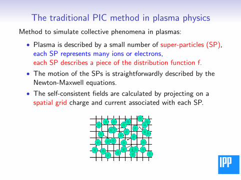
Method to simulate collective phenomena in plasmas:
• Plasma is described by a small number of super-particles (SP),each SP represents many ions or electrons,each SP describes a piece of the distribution function f.
• The motion of the SPs is straightforwardly described by theNewton-Maxwell equations.
• The self-consistent fields are calculated by projecting on aspatial grid charge and current associated with each SP.
The PIC method in general..
The PIC method is a numerical technique used to solve a certainclass of partial differential equations:
• individual particles (or fluid elements) in a Lagrangian frameare tracked in continuous phase space
• moments of the distribution function are computedsimultaneously on Eulerian (stationary) mesh points.
Solid and fluid mechanics, cosmology,...Plasma physics:laser-plasma interactions, electron acceleration and ion heating inthe auroral ionosphere, magnetic reconnection...Gyrokinetics
Outline
• Construct a set of gyrokinetic (GK) equations, suited forsimulations:
1) Must preserve symmetries: conserved quantities (energy).2) Must contain (only) relevant physics: approximation are needed,but must not break self-consistency.
General procedure: GK field theory.Example: Electrostatic, linearised polarisation GK Vlasov-Maxwell.
• PIC discretization for particle and field eqs. (finite elements).
• Properties of the discretised equations (conservation, errors,convergences,..).
• Examples, simulations of experimental plasmas.
Self-consistent gyrokinetic equation from GK Lagrangian
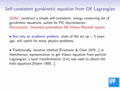
GOAL: construct a simple self-consistent, energy conserving set ofgyrokinetic equations, suited for PIC discretisation:Electrostatic, linearised polarisation GK Vlasov-Maxwell system.
• Not only an academic problem: state of the art up ∼ 5 yearsago, still useful for many physics problems.
• Traditionally, iterative method [Friemann & Chen 1979...] orHamiltonian representation to get Vlasov equation from particleLagrangian; a back transformation (Lie) was used to obtain thefield equations [Hahm 1988...].1) Establish a GK Lagrangian.
The symmetry and conservation properties are preserved.
Self-consistent gyrokinetic equation from GK Lagrangian
GOAL: construct a simple self-consistent, energy conserving set ofgyrokinetic equations, suited for PIC discretisation:Electrostatic, linearised polarisation GK Vlasov-Maxwell system
TOOL: gyrokinetic field theory.
1) Establish a proper GK Lagrangian for particles and fields.2) Approximate the Lagrangian.3) Classical field theory: derive equations for particles and fieldsfrom variational principles.4) Discretise the resulting equations using PIC.
The symmetry and conservation properties are preserved.
Self-consistent gyrokinetic equation from GK Lagrangian
GOAL: construct a simple self-consistent, energy conserving set ofgyrokinetic equations, suited for PIC discretisation.Electrostatic, linearised polarisation GK Vlasov-Maxwell system
TOOL: gyrokinetic field theory.
1) Establish a proper GK Lagrangian for particles and fields.
2) Approximate the Lagrangian.
3) Classical field theory: derive equations for particles and fieldsfrom variational principles.Discretise the resulting equations.
The symmetry and conservation properties are preserved.
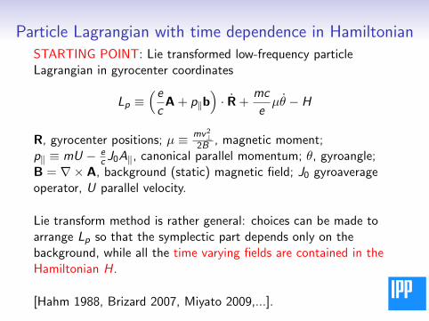
Particle Lagrangian with time dependence in HamiltonianSTARTING POINT: Lie transformed low-frequency particleLagrangian in gyrocenter coordinates
Lp ≡(ecA + p‖b
)· R +
mc
eµθ − H
R, gyrocenter positions; µ ≡ mv2⊥
2B , magnetic moment;p‖ ≡ mU − e
c J0A‖, canonical parallel momentum; θ, gyroangle;B = ∇× A, background (static) magnetic field; J0 gyroaverageoperator, U parallel velocity.
Lie transform method is rather general: choices can be made toarrange Lp so that the symplectic part depends only on thebackground, while all the time varying fields are contained in theHamiltonian H.
[Hahm 1988, Brizard 2007, Miyato 2009,...].
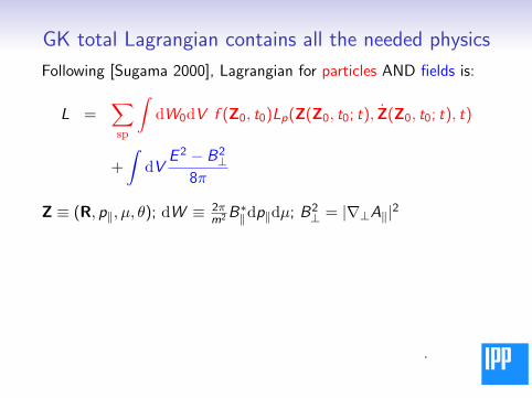
GK total Lagrangian contains all the needed physics
Following [Sugama 2000], Lagrangian for particles AND fields is:
L =∑sp
∫dW0dV f (Z0, t0)Lp(Z(Z0, t0; t), Z(Z0, t0; t), t)
+
∫dV
E 2 − B2⊥
8π
Z ≡ (R, p‖, µ, θ); dW ≡ 2πm2B
∗‖dp‖dµ; B2
⊥ = |∇⊥A‖|2 The first
term is the Lagrangian for charged particles.
•f (Z0) is the distribution function for the species sp at an arbitraryinitial time t0.•Lp is the Lie transformed particle Lagrangian written in terms ofthe gyro-center coordinates, acts as a Lagrangian density.
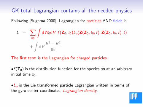
GK total Lagrangian contains all the needed physics
Following [Sugama 2000], Lagrangian for particles AND fields is:
L =∑sp
∫dW0dV f (Z0, t0)Lp(Z(Z0, t0; t), Z(Z0, t0; t), t)
+
∫dV
E 2 − B2⊥
8π
The first term is the Lagrangian for charged particles.
•f (Z0) is the distribution function for the species sp at an arbitraryinitial time t0.
•Lp is the Lie transformed particle Lagrangian written in terms ofthe gyro-center coordinates, Lagrangian density.
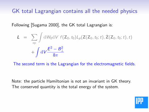
GK total Lagrangian contains all the needed physics
Following [Sugama 2000], the GK total Lagrangian is:
L =∑sp
∫dW0dV f (Z0, t0)Lp(Z(Z0, t0; t), Z(Z0, t0; t), t)
+
∫dV
E 2 − B2⊥
8π
The second term is the Lagrangian for the electromagnetic fields.
Note: the particle Hamiltonian is not an invariant in GK theory.The conserved quantity is the total energy of the system.
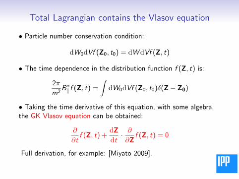
Total Lagrangian contains the Vlasov equation
• Particle number conservation condition:
dW0dVf (Z0, t0) = dWdVf (Z, t)
• The time dependence in the distribution function f (Z, t) is:
2π
m2B∗‖ f (Z, t) =
∫dW0dVf (Z0, t0)δ(Z− Z0)
• Taking the time derivative of this equation, with some algebra,the GK Vlasov equation can be obtained:
∂
∂tf (Z, t) +
dZ
dt· ∂∂Z
f (Z, t) = 0
Full derivation, for example: [Miyato 2009].
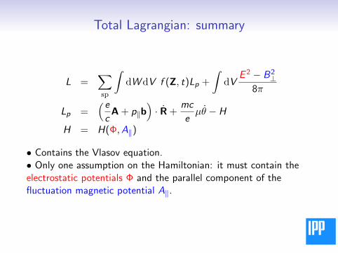
Total Lagrangian: summary
L =∑sp
∫dWdV f (Z, t)Lp +
∫dV
E 2 − B2⊥
8π
Lp =(ecA + p‖b
)· R +
mc
eµθ − H
H = H(Φ,A‖)
• Contains the Vlasov equation.• Only one assumption on the Hamiltonian: it must contain theelectrostatic potentials Φ and the parallel component of thefluctuation magnetic potential A‖.
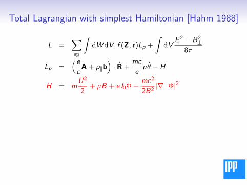
Total Lagrangian with simplest Hamiltonian [Hahm 1988]
L =∑sp
∫dWdV f (Z, t)Lp +
∫dV
E 2 − B2⊥
8π
Lp =(ecA + p‖b
)· R +
mc
eµθ − H
H = mU2
2+ µB + eJ0Φ− mc2
2B2|∇⊥Φ|2
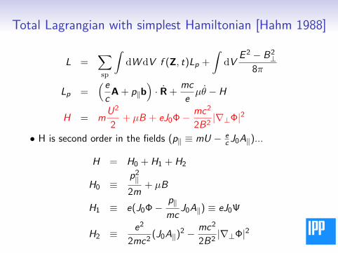
• H is second order in both fields (p‖ ≡ mU − ec J0A‖)...
H = H0 + H1 + H2
H0 ≡p2‖2m
+ µB
H1 ≡ e(J0Φ−p‖mc
J0A‖) ≡ eJ0Ψ
H2 ≡ e2
2mc2(J0A‖)
2 − mc2
2B2|∇⊥Φ|2
Total Lagrangian with simplest Hamiltonian [Hahm 1988]
L =∑sp
∫dWdV f (Z, t)Lp +
∫dV
E 2 − B2⊥
8π
Lp =(ecA + p‖b
)· R +
mc
eµθ − H
H = mU2
2+ µB + eJ0Φ− mc2
2B2|∇⊥Φ|2
• H is second order in the fields (p‖ ≡ mU − ec J0A‖)...
H = H0 + H1 + H2
H0 ≡p2‖2m
+ µB
H1 ≡ e(J0Φ−p‖mc
J0A‖) ≡ eJ0Ψ
H2 ≡ e2
2mc2(J0A‖)
2 − mc2
2B2|∇⊥Φ|2
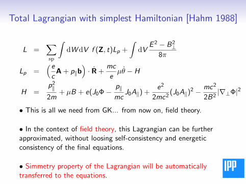
Total Lagrangian with simplest Hamiltonian [Hahm 1988]
L =∑sp
∫dWdV f (Z, t)Lp +
∫dV
E 2 − B2⊥
8π
Lp =(ecA + p‖b
)· R +
mc
eµθ − H
H =p2‖2m
+ µB + e(J0Φ−p‖mc
J0A‖) +e2
2mc2(J0A‖)
2 − mc2
2B2|∇⊥Φ|2
• This is all we need from GK... from now on, field theory.
• In the context of field theory, this Lagrangian can be furtherapproximated, without loosing self-consistency and energeticconsistency of the final equations.
• Simmetry property of the Lagrangian will be automaticallytransferred to the equations.
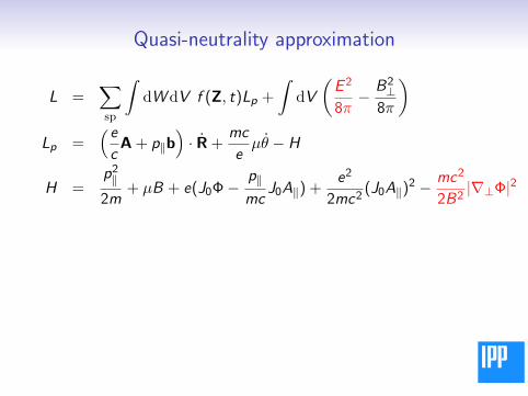
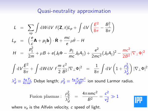
Quasi-neutrality approximation
L =∑sp
∫dWdV f (Z, t)Lp +
∫dV
(E 2
8π−
B2⊥
8π
)Lp =
(ecA + p‖b
)· R +
mc
eµθ − H
H =p2‖2m
+ µB + e(J0Φ−p‖mc
J0A‖) +e2
2mc2(J0A‖)
2 − mc2
2B2|∇⊥Φ|2
∫dV
E 2
8π+
∫dWdV f
m
2
c2
B2|∇⊥Φ|2 =
1
8π
∫dV
(1 +
ρ2Sλ2d
)|∇⊥Φ|2
λ2d ≡kBTe
4πne2Debye length; ρ2S ≡
kBTemc2
e2B2 ion sound Larmor radius.
In fusion plasmas :ρ2Sλ2d
=4πnmc2
B2=
c2
v2a 1
where va is the Alfven velocity, c speed of light.
Quasi-neutrality approximation
L =∑sp
∫dWdV f (Z, t)Lp +
∫dV
(E 2
8π−
B2⊥
8π
)Lp =
(ecA + p‖b
)· R +
mc
eµθ − H
H =p2‖2m
+ µB + e(J0Φ−p‖mc
J0A‖) +e2
2mc2(J0A‖)
2 − mc2
2B2|∇⊥Φ|2
∫dV
E 2
8π+
∫dWdV f
m
2
c2
B2|∇⊥Φ|2 =
1
8π
∫dV
(1 +
ρ2Sλ2d
)|∇⊥Φ|2
λ2d ≡kBTe
4πne2Debye length; ρ2S ≡
kBTemc2
e2B2 ion sound Larmor radius.
Fusion plasmas :ρ2Sλ2d
=4πnmc2
B2=
c2
v2a 1
where va is the Alfven velocity, c speed of light.
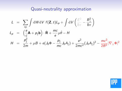
Quasi-neutrality approximation
L =∑sp
∫dWdV f (Z, t)Lp +
∫dV
(E 2
8π−
B2⊥
8π
)Lp =
(ecA + p‖b
)· R +
mc
eµθ − H
H =p2‖2m
+ µB + e(J0Φ−p‖mc
J0A‖) +e2
2mc2(J0A‖)
2 − mc2
2B2|∇⊥Φ|2
∫dV
E 2
8π+
∫dWdV f
m
2
c2
B2|∇⊥Φ|2 =
1
8π
∫dV
(1 +
ρ2Sλ2d
)|∇⊥Φ|2
λ2d ≡kBTe
4πne2Debye length; ρ2S ≡
kBTemc2
e2B2 ion sound Larmor radius.
In fusion plasmas :ρ2Sλ2d
=4πnmc2
B2=
c2
v2a 1
where va is the Alfven velocity, c speed of light.
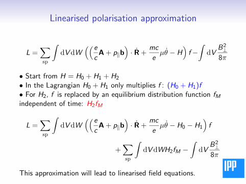
Linearised polarisation approximation
L =∑sp
∫dVdW
((ecA + p‖b
)· R +
mc
eµθ − H
)f−∫
dVB2⊥
8π
• Start from H = H0 + H1 + H2
• In the Lagrangian H0 + H1 only multiplies f : (H0 + H1)f• For H2, f is replaced by an equilibrium distribution function fMindependent of time: H2fM
L =∑sp
∫dVdW
((ecA + p‖b
)· R +
mc
eµθ − H0 − H1
)f
+∑sp
∫dVdWH2fM −
∫dV
B2⊥
8π
This approximation will lead to linearised field equations.
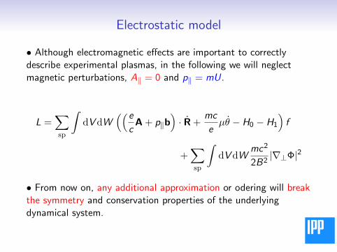
Electrostatic model
• Although electromagnetic effects are important to correctlydescribe experimental plasmas, in the following we will neglectmagnetic perturbations, A‖ = 0 and p‖ = mU.
L =∑sp
∫dVdW
((ecA + p‖b
)· R +
mc
eµθ − H0 − H1
)f
+∑sp
∫dVdW
mc2
2B2|∇⊥Φ|2
• From now on, any additional approximation or odering will breakthe symmetry and conservation properties of the underlyingdynamical system.
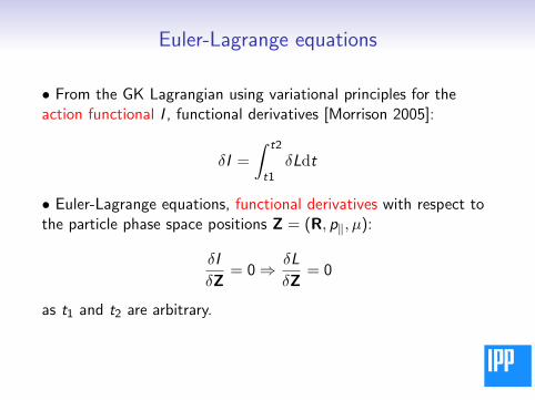
Euler-Lagrange equations
• From the GK Lagrangian using variational principles for theaction functional I , functional derivatives [Morrison 2005]:
δI =
∫ t2
t1δLdt
• Euler-Lagrange equations, functional derivatives with respect tothe particle phase space positions Z = (R, p‖, µ):
δI
δZ= 0⇒ δL
δZ= 0
as t1 and t2 are arbitrary.
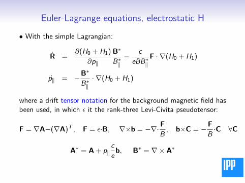
Euler-Lagrange equations, electrostatic H
• With the simple Lagrangian:
R =∂(H0 + H1)
∂p‖
B∗
B∗‖− c
eBB∗‖F · ∇(H0 + H1)
p‖ = −B∗
B∗‖· ∇(H0 + H1)
where a drift tensor notation for the background magnetic field hasbeen used, in which ε it the rank-three Levi-Civita pseudotensor:
F = ∇A−(∇A)T , F = ε·B, ∇×b = −∇·FB, b×C = −F
B·C ∀C
A∗ = A + p‖c
eb, B∗ = ∇× A∗
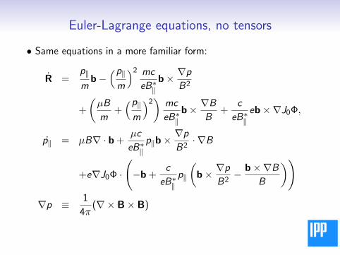
Euler-Lagrange equations, no tensors
• Same equations in a more familiar form:
R =p‖mb−
(p‖m
)2 mc
eB∗‖b× ∇p
B2
+
(µB
m+(p‖m
)2) mc
eB∗‖b× ∇B
B+
c
eB∗‖eb×∇J0Φ,
p‖ = µB∇ · b +µc
eB∗‖p‖b×
∇pB2· ∇B
+e∇J0Φ ·
(−b +
c
eB∗‖p‖
(b× ∇p
B2− b×∇B
B
))∇p ≡ 1
4π(∇× B× B)
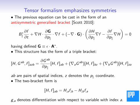
Tensor formalism emphasizes symmetries• The previous equation can be cast in the form of anantisymmetric generalised bracket [Scott 2010]:
B∗‖∂f
∂t+∇H · ∂G
∂p‖· ∇f + (−∇ · G) ·
(∂H
∂p‖∇f − ∂f
∂p‖∇H
)= 0
having defined G ≡ ε · A∗.• This structure has the form of a triple bracket:
[H,G ab, f ]azb =∂G ab
∂p‖[H, f ]ab + (∇aG
ab)[H, f ]bz + (∇bGab)[H, f ]za
ab are pairs of spatial indices, z denotes the p‖ coordinate.• The two-bracket form is
[H, f ]ab = H,af,b − H,bf,a
g,a denotes differentiation with respect to variable with index a.
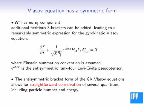
Vlasov equation has a symmetric form
• A∗ has no p‖ component:additional fictitious 3-brackets can be added, leading to aremarkably symmetric expression for the gyrokinetic Vlasovequation.
∂f
∂t+
1√gB∗‖
εabczH,af,bA∗c,z = 0
where Einstein summation convention is assumed.εabcz is the antisymmetric rank-four Levi-Civita pseudotensor.
• The antisymmetric bracket form of the GK Vlasov equationsallows for straightforward conservation of several quantities,including particle number and energy.
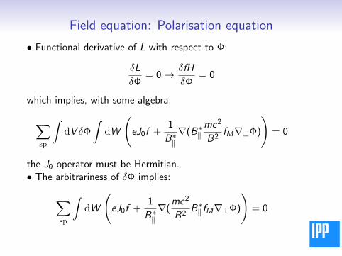
Field equation: Polarisation equation
• Functional derivative of L with respect to Φ:
δL
δΦ= 0→ δfH
δΦ= 0
which implies, with some algebra,
∑sp
∫dV δΦ
∫dW
(eJ0f +
1
B∗‖∇(B∗‖
mc2
B2fM∇⊥Φ)
)= 0
the J0 operator must be Hermitian.• The arbitrariness of δΦ implies:
∑sp
∫dW
(eJ0f +
1
B∗‖∇(
mc2
B2B∗‖ fM∇⊥Φ)
)= 0
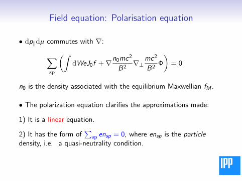
Field equation: Polarisation equation
• dp‖dµ commutes with ∇:
∑sp
(∫dWeJ0f +∇n0mc2
B2∇⊥
mc2
B2Φ
)= 0
n0 is the density associated with the equilibrium Maxwellian fM .
• The polarization equation clarifies the approximations made:
1) It is a linear equation.
2) It has the form of∑
sp ensp = 0, where ensp is the particledensity, i.e. a quasi-neutrality condition.
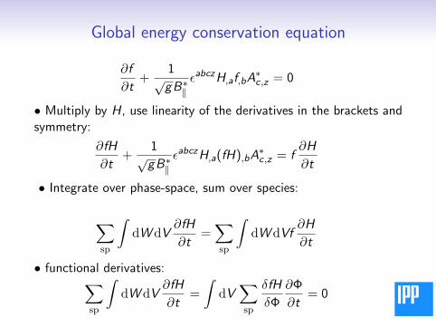
Global energy conservation equation
∂f
∂t+
1√gB∗‖
εabczH,af,bA∗c,z = 0
• Multiply by H, use linearity of the derivatives in the brackets andsymmetry:
∂fH
∂t+
1√gB∗‖
εabczH,a(fH),bA∗c,z = f
∂H
∂t
• Integrate over phase-space, sum over species:
∑sp
∫dWdV
∂fH
∂t=∑sp
∫dWdVf
∂H
∂t
• functional derivatives:∑sp
∫dWdV
∂fH
∂t=
∫dV∑sp
δfH
δΦ
∂Φ
∂t= 0
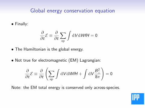
Global energy conservation equation
• Finally:
∂
∂tE ≡ ∂
∂t
∑sp
∫dVdWfH = 0
• The Hamiltonian is the global energy.
• Not true for electromagnetic (EM) Lagrangian:
∂
∂tE ≡ ∂
∂t
(∑sp
∫dVdWfH +
∫dV
B2⊥
8π
)= 0
Note: the EM total energy is conserved only across-species.
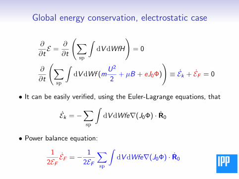
Global energy conservation, electrostatic case
∂
∂tE =
∂
∂t
(∑sp
∫dVdWfH
)= 0
∂
∂t
(∑sp
∫dVdWf (m
U2
2+ µB + eJ0Φ)
)≡ Ek + EF = 0
• It can be easily verified, using the Euler-Lagrange equations, that
Ek = −∑sp
∫dVdWfe∇(J0Φ) · R0
• Power balance equation:
1
2EFEF = − 1
2EF
∑sp
∫dVdWfe∇(J0Φ) · R0
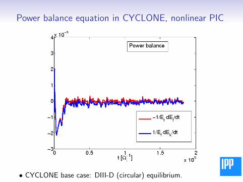
Power balance equation in CYCLONE, nonlinear PIC
• CYCLONE base case: DIII-D (circular) equilibrium.
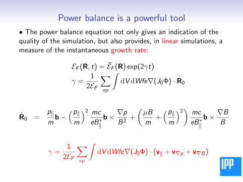
Power balance is a powerful tool
• The power balance equation not only gives an indication of thequality of the simulation, but also provides, in linear simulations, ameasure of the instantaneous growth rate:
EF (R, t) = EF (R) exp(2γt)
γ =1
2EF
∑sp
∫dVdWfe∇(J0Φ) · R0
R0 =p‖mb−
(p‖m
)2 mc
eB∗‖b× ∇p
B2+
(µB
m+(p‖m
)2) mc
eB∗‖b× ∇B
B
γ =1
2EF
∑sp
∫dVdWfe∇(J0Φ) · (v‖ + v∇p + v∇B)
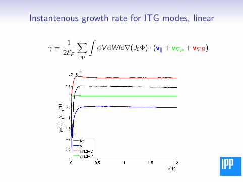
Instantenous growth rate for ITG modes, linear
γ =1
2EF
∑sp
∫dVdWfe∇(J0Φ) · (v‖ + v∇p + v∇B)
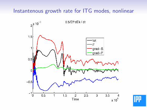
Instantenous growth rate for ITG modes, nonlinear
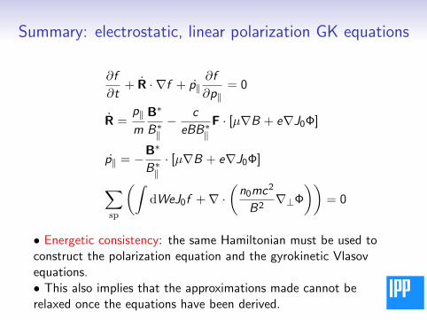
Summary: electrostatic, linear polarization GK equations
∂f
∂t+ R · ∇f + p‖
∂f
∂p‖= 0
R =p‖m
B∗
B∗‖− c
eBB∗‖F · [µ∇B + e∇J0Φ]
p‖ = −B∗
B∗‖· [µ∇B + e∇J0Φ]
∑sp
(∫dWeJ0f +∇ ·
(n0mc2
B2∇⊥Φ
))= 0
• Energetic consistency: the same Hamiltonian must be used toconstruct the polarization equation and the gyrokinetic Vlasovequations.• This also implies that the approximations made cannot berelaxed once the equations have been derived.
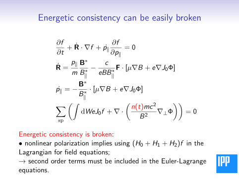
Energetic consistency can be easily broken
∂f
∂t+ R · ∇f + p‖
∂f
∂p‖= 0
R =p‖m
B∗
B∗‖− c
eBB∗‖F · [µ∇B + e∇J0Φ]
p‖ = −B∗
B∗‖· [µ∇B + e∇J0Φ]
∑sp
(∫dWeJ0f +∇ ·
(n(t)mc2
B2∇⊥Φ
))= 0
Energetic consistency is broken:• nonlinear polarization implies using (H0 + H1 + H2)f in theLagrangian for field equations;→ second order terms must be included in the Euler-Lagrangeequations.

Energetic consistency can be easily broken
∂f
∂t+ R · ∇f + p‖
∂f
∂p‖= 0
R =p‖m
B∗
B∗‖− c
eBB∗‖F · [µ∇B + e∇J0Φ] + O(Φ2)
p‖ = −B∗
B∗‖· [µ∇B + e∇J0Φ] + O(Φ2)
∑sp
(∫dWeJ0f +∇ ·
(n(t)mc2
B2∇⊥Φ
))= 0
Energetic consistency is restored:• nonlinear polarization implies using (H0 + H1 + H2)f in theLagrangian for field equations;→ second order terms must be included in the Euler-Lagrangeequations.
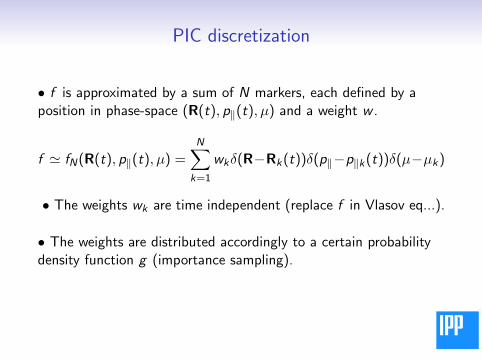
PIC discretization
• f is approximated by a sum of N markers, each defined by aposition in phase-space (R(t), p‖(t), µ) and a weight w .
f ' fN(R(t), p‖(t), µ) =N∑
k=1
wkδ(R−Rk(t))δ(p‖−p‖k(t))δ(µ−µk)
• The weights wk are time independent (replace f in Vlasov eq...).
• The weights are distributed accordingly to a certain probabilitydensity function g (importance sampling).
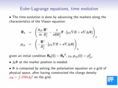
Euler-Lagrange equations, time evolution
• The time evolution is done by advancing the markers along thecharacteristics of the Vlasov equation:
Rk =
(p‖km
B∗
B∗‖− c
eBB∗‖F · [µk∇B + e∇J0Φ]
)k
˙p‖k =
(−B∗
B∗‖· [µk∇B + e∇J0Φ]
)k
given an initial condition Rk(0) = Rk0, µk ,p‖k(0) = p0‖k .
• J0Φ at the marker position is needed.
• Φ is computed by solving the polarisation equation on a grid ofphysical space, after having constructed the charge densityρN =
∫dWeJ0f on the grid.
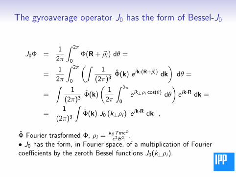
The gyroaverage operator J0 has the form of Bessel-J0
J0Φ =1
2π
∫ 2π
0Φ(R + ~ρi ) dθ =
=1
2π
∫ 2π
0
(∫1
(2π)3Φ(k) e ik·(R+~ρi ) dk
)dθ =
=
∫1
(2π)3Φ(k)
(1
2π
∫ 2π
0e ik⊥ρi cos(θ) dθ
)e ik·R dk =
=1
(2π)3
∫Φ(k) J0 (k⊥ρi ) e ik·R dk ,
Φ Fourier trasformed Φ, ρi = kBTmc2
e2B2 .• J0 has the form, in Fourier space, of a multiplication of Fouriercoefficients by the zeroth Bessel functions J0(k⊥ρi ).
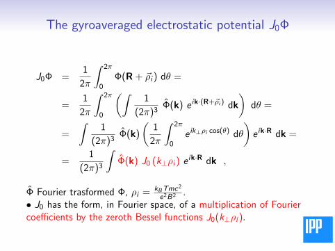
The gyroaveraged electrostatic potential J0Φ
J0Φ =1
2π
∫ 2π
0Φ(R + ~ρi ) dθ =
=1
2π
∫ 2π
0
(∫1
(2π)3Φ(k) e ik·(R+~ρi ) dk
)dθ =
=
∫1
(2π)3Φ(k)
(1
2π
∫ 2π
0e ik⊥ρi cos(θ) dθ
)e ik·R dk =
=1
(2π)3
∫Φ(k) J0 (k⊥ρi ) e ik·R dk ,
Φ Fourier trasformed Φ, ρi = kBTmc2
e2B2 .• J0 has the form, in Fourier space, of a multiplication of Fouriercoefficients by the zeroth Bessel functions J0(k⊥ρi ).
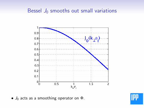
Bessel J0 smooths out small variations
• J0 acts as a smoothing operator on Φ.
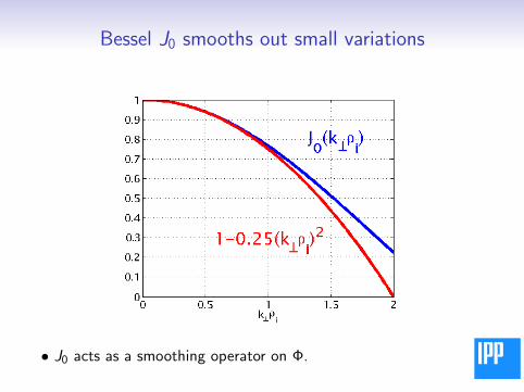
Bessel J0 smooths out small variations
• J0 acts as a smoothing operator on Φ.
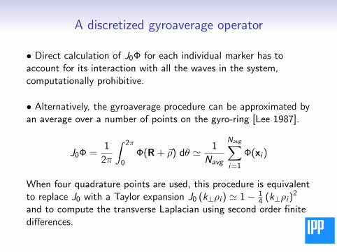
A discretized gyroaverage operator
• Direct calculation of J0Φ for each individual marker has toaccount for its interaction with all the waves in the system,computationally prohibitive.
• Alternatively, the gyroaverage procedure can be approximated byan average over a number of points on the gyro-ring [Lee 1987].
J0Φ =1
2π
∫ 2π
0Φ(R + ~ρ) dθ ' 1
Navg
Navg∑i=1
Φ(xi )
When four quadrature points are used, this procedure is equivalentto replace J0 with a Taylor expansion J0 (k⊥ρi ) ' 1− 1
4 (k⊥ρi )2
and to compute the transverse Laplacian using second order finitedifferences.
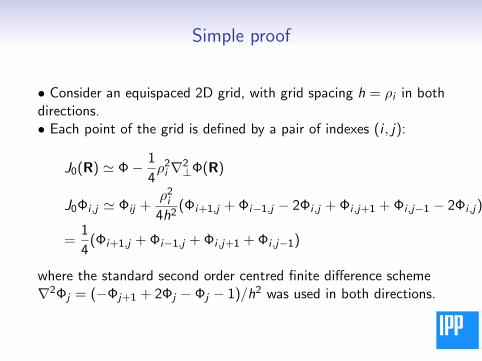
Simple proof
• Consider an equispaced 2D grid, with grid spacing h = ρi in bothdirections.• Each point of the grid is defined by a pair of indexes (i , j):
J0(R) ' Φ− 1
4ρ2i∇2
⊥Φ(R)
J0Φi ,j ' Φij +ρ2i
4h2(Φi+1,j + Φi−1,j − 2Φi ,j + Φi ,j+1 + Φi ,j−1 − 2Φi ,j)
=1
4(Φi+1,j + Φi−1,j + Φi ,j+1 + Φi ,j−1)
where the standard second order centred finite difference scheme∇2Φj = (−Φj+1 + 2Φj − Φj − 1)/h2 was used in both directions.
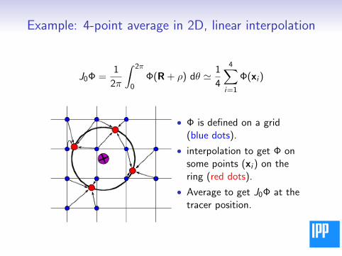
Example: 4-point average in 2D, linear interpolation
J0Φ =1
2π
∫ 2π
0Φ(R + ρ) dθ ' 1
4
4∑i=1
Φ(xi )
• Φ is defined on a grid(blue dots).
• interpolation to get Φ onsome points (xi ) on thering (red dots).
• Average to get J0Φ at thetracer position.
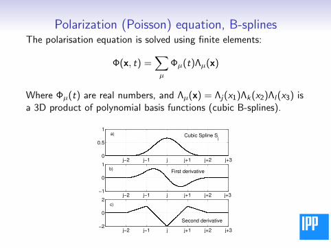
Polarization (Poisson) equation, B-splinesThe polarisation equation is solved using finite elements:
Φ(x, t) =∑µ
Φµ(t)Λµ(x)
Where Φµ(t) are real numbers, and Λµ(x) = Λj(x1)Λk(x2)Λl(x3) isa 3D product of polynomial basis functions (cubic B-splines).
j−2 j−1 j j+1 j+2 j+30
0.5
1
j−2 j−1 j j+1 j+2 j+3 −1
0
1
j−2 j−1 j j+1 j+2 j+3−2
0
2
Cubic Spline Sj
First derivative
Second derivative
a)
b)
c)
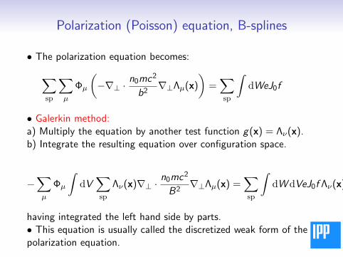
Polarization (Poisson) equation, B-splines
• The polarization equation becomes:∑sp
∑µ
Φµ
(−∇⊥ ·
n0mc2
b2∇⊥Λµ(x)
)=∑sp
∫dWeJ0f
• Galerkin method:a) Multiply the equation by another test function g(x) = Λν(x).b) Integrate the resulting equation over configuration space.
−∑µ
Φµ
∫dV∑sp
Λν(x)∇⊥ ·n0mc2
B2∇⊥Λµ(x) =
∑sp
∫dWdVeJ0f Λν(x) (1)
having integrated the left hand side by parts.• This equation is usually called the discretized weak form of thepolarization equation.
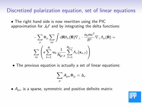
Discretized polarization equation, set of linear equations
• The right hand side is now rewritten using the PICapproximation for J0f and by integrating the delta functions:
−∑µ
Φµ
∑sp
∫dRΛν(R)∇⊥ ·
n0mc2
B2∇⊥Λµ(R) =
∑sp
eN∑
k=1
wk1
Ngr ,k
Ngr,k∑β=1
Λν(xk,β)
• The previous equation is actually a set of linear equations:∑
µ
AµνΦµ = bν
• Aµν is a sparse, symmetric and positive definite matrix
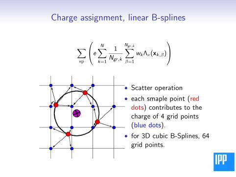
Charge assignment, linear B-splines
∑sp
eN∑
k=1
1
Ngr ,k
Ngr,k∑β=1
wkΛν(xk,β)
• Scatter operation
• each smaple point (reddots) contributes to thecharge of 4 grid points(blue dots).
• for 3D cubic B-Splines, 64grid points.
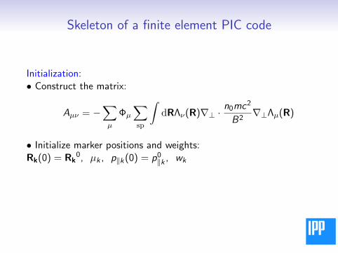
Skeleton of a finite element PIC code
Initialization:• Construct the matrix:
Aµν = −∑µ
Φµ
∑sp
∫dRΛν(R)∇⊥ ·
n0mc2
B2∇⊥Λµ(R)
• Initialize marker positions and weights:Rk(0) = Rk
0, µk , p‖k(0) = p0‖k , wk
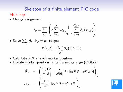
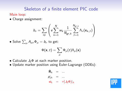
Skeleton of a finite element PIC codeMain loop:• Charge assignment:
bν =∑sp
eN∑
k=1
wk1
Ngr ,k
Ngr,k∑β=1
Λν(xk,β)
• Solve
∑µ AµνΦµ = bν to get:
Φ(x, t) =∑µ
Φµ(t)Λµ(x)
• Calculate J0Φ at each marker position.• Update marker position using Euler-Lagrange (ODEs):
Rk =
(p‖km
B∗
B∗‖− c
eBB∗‖F · [µk∇B + e∇J0Φ]
)k
˙p‖k =
(−B∗
B∗‖· [µk∇B + e∇J0Φ]
)k
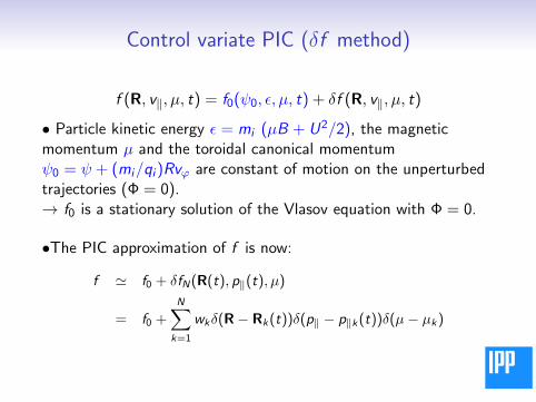
Control variate PIC (δf method)
f (R, v‖, µ, t) = f0(ψ0, ε, µ, t) + δf (R, v‖, µ, t)
• Particle kinetic energy ε = mi (µB + U2/2), the magneticmomentum µ and the toroidal canonical momentumψ0 = ψ + (mi/qi )Rvϕ are constant of motion on the unperturbedtrajectories (Φ = 0).→ f0 is a stationary solution of the Vlasov equation with Φ = 0.
•The PIC approximation of f is now:
f ' f0 + δfN(R(t), p‖(t), µ)
= f0 +N∑
k=1
wkδ(R− Rk(t))δ(p‖ − p‖k(t))δ(µ− µk)
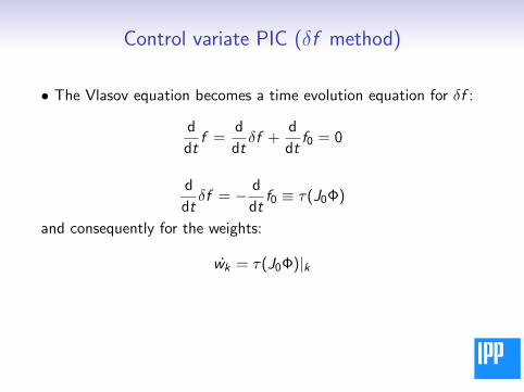
Control variate PIC (δf method)
• The Vlasov equation becomes a time evolution equation for δf :
d
dtf =
d
dtδf +
d
dtf0 = 0
d
dtδf = − d
dtf0 ≡ τ(J0Φ)
and consequently for the weights:
wk = τ(J0Φ)|k
Skeleton of a finite element PIC codeMain loop:• Charge assignment:
bν =∑sp
eN∑
k=1
wk1
Ngr ,k
Ngr,k∑β=1
Λν(xk,β)
• Solve
∑µ AµνΦµ = bν to get:
Φ(x, t) =∑µ
Φµ(t)Λµ(x)
• Calculate J0Φ at each marker position.• Update marker position using Euler-Lagrange (ODEs):
Rk = ...
˙p‖k = ...
wk = τ(J0Φ)|k

Simple Monte-Carlo estimate for the noise
• Statistical noise (Aydemir 1994):Error ε introduced when the moment of the distributionfunction (density) is evaluated with a finite number N ofparticles, ε ' σ/
√N
ρ2noise 'NG
N〈w2〉G ; 〈w2〉 ≡ 1
N
N∑i=1
w2i
NG , number of Fourier modes included in the simulation.G accounts for FLR filtering and grid projection filtering.
• Noise can be reduced by:1. Increasing the number of tracers N.2. Reducing the number of modes NG → Fourier filtering.3. Reducing 〈w2〉 (MC, reducing σ)4. Carefully choosing the projection algorithm, i.e. G .
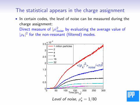
The statistical appears in the charge assignment
• In certain codes, the level of noise can be measured during thecharge assignment:Direct measure of |ρ|2noise by evaluating the average value of|ρk |2 for the non-resonant (filtered) modes.
0 50 100 150 200 250 3000
0.5
1
1.5
2
2.5
3
3.5x 10
−4
Time [a/vTe
]
1 milion particles 2481632
<|ρk|2>
noise/<n>2
Level of noise, ρ∗e = 1/80
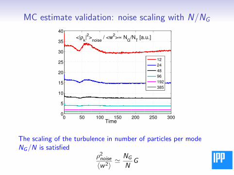
MC estimate validation: noise scaling with N/NG
0 50 100 150 200 250 3000
5
10
15
20
25
30
35
40
Time
12244896192385
<|ρk|2>
noise / <w2>∝ N
G/N
T [a.u.]
The scaling of the turbulence in number of particles per modeNG/N is satisfied
ρ2noise〈w2〉
' NG
NG
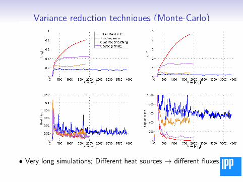
Variance reduction techniques (Monte-Carlo)
• Very long simulations; Different heat sources → different fluxes.
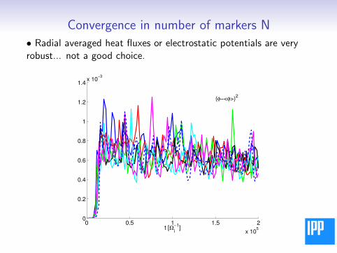
Convergence in number of markers N
• Radial averaged heat fluxes or electrostatic potentials are veryrobust... not a good choice.
0 0.5 1 1.5 2
x 105
0
0.2
0.4
0.6
0.8
1
1.2
1.4x 10
−3
(φ−<φ>)2
t [Ωi
−1]
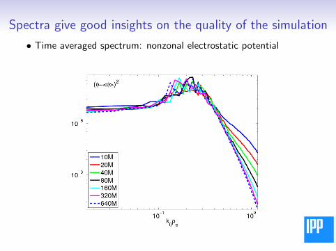
Spectra give good insights on the quality of the simulation
• Time averaged spectrum: nonzonal electrostatic potential
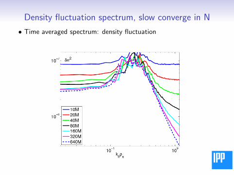
Density fluctuation spectrum, slow converge in N
• Time averaged spectrum: density fluctuation
References (1)
AYDEMIR, AHMET Y. 1994 A unified monte carlo interpretation ofparticle simulations and applications to non-neutral plasmas. Physics ofPlasmas 1 (4), 822-831.BRIZARD, A., HAHM, T.S. 2007 Foundations of nonlinear gyrokinetictheory. Rev. Mod. Phys. 79, 421.FRIEMAN, E. A., CHEN, L. 1982 Nonlinear gyrrokinetic equations forlow frequency electromagnetic waves in general equilibria. Physics ofFluids 25, 502.HAHM, T. S. 1988 Nonlinear gyrokinetic equations for tokamakmicroturbulence. Physics of Fluids 31, 2670.LEE, W. W. 1983 Gyrokinetic approach in particle simulations. Physicsof Fluids 26, 556.Lee, W W 1987 Gyrokinetic particle simulation model. Journal ofComputational Physics 73, 243.
References (2)
MIYATO, N., SCOTT, B., STRINTZI, D. 2009 A modification of theguiding-centre fundamental 1-form with strong ExB flow. J. Phys. Soc.Jpn. 78, 104501.SCOTT, B., KENDL, A., RIBEIRO, T. 2010 Nonlinear dynamics in thetokamak edge. Contrib. Plasma Phys. 50, 228.SCOTT, B., SMIRNOV, J. 2010 Energetic consistency and momentumconservation in the gyrokinetic description of tokamak plasmas. Physicsof Plasmas 17, 112302.SUGAMA, H. 2000 Gyrokinetic field theory. Physics of Plasmas 7, 466.
• All the simulations were performed with the ORB5 (NEMORB) code:JOLLIET, S., BOTTINO, A., ANGELINO, P. et al. 2007 A globalcollisionless PIC code in magnetic coordinates. Computer PhysicsCommunications 177, 409.BOTTINO, A., SCOTT, B., BRUNNER, S. et al. 2010 Global nonlinearelectromagnetic simulations of tokamak turbulence. IEEE Transactionson Plasma Science 38, 2129.