Embed Size (px)
Citation preview
Summer school on “Measuring techniques for turbulent open-channel flows”
Introduction to particle-based methods Key principles and hardware
Summer school on “Measuring techniques for turbulent open-channel flows” Lisboa, 28-30 July 2015
Rui M.L. Ferreira, Rui Aleixo
Instituto Superior Técnico, Universidade de Lisboa; GHT Photonics
Summer school on “Measuring techniques for turbulent open-channel flows”
Motivation
“Scientific observation is always a polemic observation […]. Naturally, passing from observation to experimentation, the polemic character of knowledge becomes clearer. It is necessary that the phenomenon is isolated, filtered, shaped by the instruments; it may be that instruments produce the phenomenon in the first place. And instruments are nothing but materialized theories. It results that phenomena bear the stamp of theory throughout”
Gaston Bachelard Le nouvel esprit scientifique, p. 12-13

Summer school on “Measuring techniques for turbulent open-channel flows”
Outline
- Basic ideas behind PIV and PTV (Eulerian/lagrangian flow descriptions)
- Particle-based methods
- Necessary hardware
- Basics of PIV
- Basics of PTV

Summer school on “Measuring techniques for turbulent open-channel flows”
basic ideas
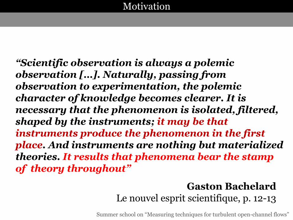
Flow description
Particle Image Velocimetry (PIV) Particle Tracking Velocimetry (PTV)
Particle-based methods and optical methods
optical methods – particle-based, light scattering from tracers (as old as photography itself)
Percival Lowell – search for planet X Clyde Tombaugh – finding Pluto
Milton van Dyke – an album of fluid motion
Onera, 1974

Summer school on “Measuring techniques for turbulent open-channel flows”
How to measure fluid velocities?
Use tracers that follow the flow. Track the tracers with imaging techniques Determine tracers displacement (each tracer or its representative velocity in a small spatial domain) Determine tracers velocity
𝐯𝑝 = 𝐯𝑓
basic ideas
Flow description

Summer school on “Measuring techniques for turbulent open-channel flows”
basic ideas
Flow description
PIV – spatial (eulerian) flow description
PTV – material (lagrangian) flow description or spatial flow description

Summer school on “Measuring techniques for turbulent open-channel flows”
basic ideas
Flow description
PIV – spatial (eulerian) flow description
PTV – material (lagrangian) flow description or spatial flow description
Spatial (eulerian) description
1 2 3, , , ,jx t x x x t B B B

Summer school on “Measuring techniques for turbulent open-channel flows”
basic ideas
Flow description
PIV – spatial (eulerian) flow description
PTV – material (lagrangian) flow description or spatial flow description
Material (Lagrangean) formulation
1 2 3, , , ,jX t X X X t B B B
,0 ,0j jx XB B

Summer school on “Measuring techniques for turbulent open-channel flows”
basic ideas
Flow description
PIV – velocity is determined as a field variable; vector tangent to small displacements in any space location, concept of streamline
PTV – velocities of each parcel of continuum are determined by (lagrangian) by diferentiation of property position, concept of pathline
d 0 u l
D d
D djXt t t
B B B
Material derivative
jxB
d 0ijk i je u l
d
d
j
j
xu
t

Summer school on “Measuring techniques for turbulent open-channel flows”
basic ideas
Flow description
PIV – velocity is determined as a field variable; vector tangent to small displacements in any space location, concept of streamline
PTV – velocities of each parcel of continuum are determined by (lagrangian) by diferentiation of property position, concept of pathline
d 0 u l
Velocity estimate
d 0ijk i je u l
0 0
22
0
0 0 2
d d...
d 2!d
j j
j j
t t
x x t tx t x t t t
t t
0
0
0
0
d
d
j j j
t
x x t x tO t t
t t t
0
0
j j
j
x t x tu
t t

Summer school on “Measuring techniques for turbulent open-channel flows”
basic ideas
Flow description
Spatial and material flowlines are not the same in unsteady flows
Summer school on “Measuring techniques for turbulent open-channel flows”
basic ideas
Flow description
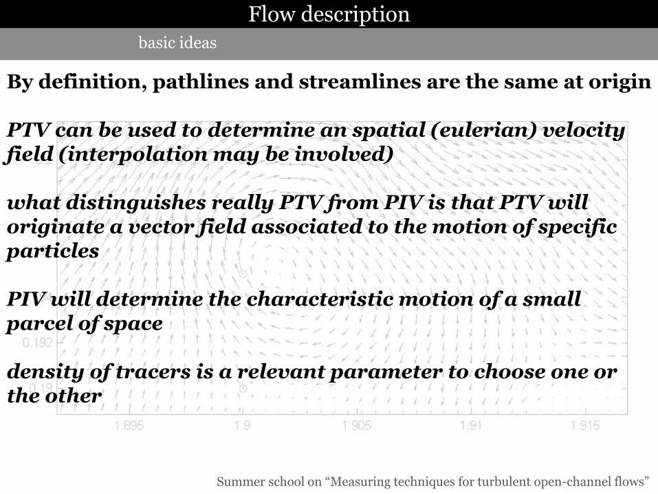
By definition, pathlines and streamlines are the same at origin
Summer school on “Measuring techniques for turbulent open-channel flows”
basic ideas
Flow description
By definition, pathlines and streamlines are the same at origin PTV can be used to determine an spatial (eulerian) velocity field (interpolation may be involved) what distinguishes really PTV from PIV is that PTV will originate a vector field associated to the motion of specific particles PIV will determine the characteristic motion of a small parcel of space density of tracers is a relevant parameter to choose one or the other

Summer school on “Measuring techniques for turbulent open-channel flows”
Questions:
Which tracers to use? How to see the tracers in the flow? How to determine the displacements?
basic ideas
Flow description

Summer school on “Measuring techniques for turbulent open-channel flows”
raw PIV image mean velocity field mean vorticity field and streamlines
the objective:
basic ideas
Flow description

Summer school on “Measuring techniques for turbulent open-channel flows”
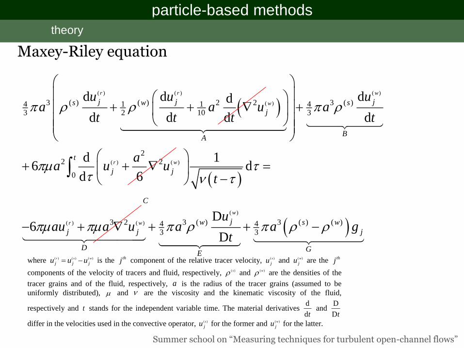
Maxey-Riley equation
( ) ( ) ( )
( )
( ) ( )
( ) ( )
3 ( ) ( ) 2 2 3 ( )4 1 1 43 2 10 3
22 2
0
3 2
d d dd
d d d d
d 16 d
d 6
6
r r w
w
r w
r w
j j js w s
j
BA
t
j j
C
j j
D
u u ua a u a
t t t t
aa u u
t
au a u
( )
3 ( ) 3 ( ) ( )4 43 3
D
D
w
jw s w
j
GE
ua a g
t
particle-based methods
theory

Summer school on “Measuring techniques for turbulent open-channel flows”
( ) ( ) ( )
( )
( ) ( )
( ) ( )
3 ( ) ( ) 2 2 3 ( )4 1 1 43 2 10 3
22 2
0
3 2
d d dd
d d d d
d 16 d
d 6
6
r r w
w
r w
r w
j j js w s
j
BA
t
j j
C
j j
D
u u ua a u a
t t t t
aa u u
t
au a u
( )
3 ( ) 3 ( ) ( )4 43 3
D
D
w
jw s w
j
GE
ua a g
t
where ( ) ( ) ( )r s w
j j ju u u is the thj component of the relative tracer velocity, ( )s
ju and ( )w
ju are the thj 1
components of the velocity of tracers and fluid, respectively, ( )s and ( )w are the densities of the 2
tracer grains and of the fluid, respectively, a is the radius of the tracer grains (assumed to be 3
uniformly distributed), and are the viscosity and the kinematic viscosity of the fluid, 4
respectively and t stands for the independent variable time. The material derivatives d
dt and
D
Dt5
differ in the velocities used in the convective operator, ( )s
ju for the former and ( )w
ju for the latter. 6
Maxey-Riley equation
added mass
Basset history term
viscous drag flow gradients buoyancy
particle-based methods
theory
Summer school on “Measuring techniques for turbulent open-channel flows”
( ) ( ) ( )
( )
( ) ( )
( ) ( )
3 ( ) ( ) 2 2 3 ( )4 1 1 43 2 10 3
22 2
0
3 2
d d dd
d d d d
d 16 d
d 6
6
r r w
w
r w
r w
j j js w s
j
BA
t
j j
C
j j
D
u u ua a u a
t t t t
aa u u
t
au a u
( )
3 ( ) 3 ( ) ( )4 43 3
D
D
w
jw s w
j
GE
ua a g
t
where ( ) ( ) ( )r s w
j j ju u u is the thj component of the relative tracer velocity, ( )s
ju and ( )w
ju are the thj 1
components of the velocity of tracers and fluid, respectively, ( )s and ( )w are the densities of the 2
tracer grains and of the fluid, respectively, a is the radius of the tracer grains (assumed to be 3
uniformly distributed), and are the viscosity and the kinematic viscosity of the fluid, 4
respectively and t stands for the independent variable time. The material derivatives d
dt and
D
Dt5
differ in the velocities used in the convective operator, ( )s
ju for the former and ( )w
ju for the latter. 6
Maxey-Riley equation
particle-based methods
theory

Summer school on “Measuring techniques for turbulent open-channel flows”
Ferreira (2015) Principles of LDA instrumentation. In IAHR Monograph Experimetal techniques
modifyed Hjemfelt & Mockros (1966)
95% confidence
cut off frequency > 105 Hz
> LDA frequency (300 Hz)
122 2
1 21Ar
( ) ( )/s w
Ar u u
1 12 2
1 2 2
21 1 12 2 2
9 31
2
9 918
4
ff f
s s
f ff
s a s s
21 1 12 2 2
2 2 2
21 1 12 2 2
918 31
4 2
9 918
4
ff
s a s s
f ff
s a s s
silica powder ( 25.0a µm, 2.65s ). 1
air bubbles ( 0.5a µm, 0.0013s ) 1
titanium dioxide ( 0.5a µm, 4.20s ) 1
seeding requirements: solution of Maxey-Riley equation
key issue of particle-based methods
particle-based methods
theory

Summer school on “Measuring techniques for turbulent open-channel flows”
seeding requirements
Example of tracer particles. Top: general view and micrographs of polyamide Dp= 50 μm, s = 1.03.
Bottom: micrograph (100x) of polyurethane beads; left: decosoft© 60 transparent beads (refractive index 1.5,
s = 1.05); right: decosoft© 60 white beads (refractive index 2.1, s = 1.3).
particle-based methods
tracers
Should be chemical inert, non-toxic and cheap

Summer school on “Measuring techniques for turbulent open-channel flows”
Table 1. Common tracer particles for LDA. 1
Mean
diameter
µm
Refractive
index
Density
(g/cm3)
Shape
Titanium dioxide 0.1 - 50.0 2.60 4.3 Irregular
Silicon carbide 1.5 2.65 3.2 Irregular
Nylon 4.0 1.53 1.14 Spherical
Metallic coated hollow glass spheres 14.0 0.21+i2.62 1.65 Spherical
Polystyrene latex 0.5 1.6 1.05 Spherical
Zirconium Oxide 30.0 2.2 5.7 Irregular
Polyurethane beads 5.0-150.0 1.5-2.1 1.05-1.3 Irregular
Air bubbles 0.1-… 1.0 1.3x10⁻³
Spherical
2
Larger particles stronger scattering lower tracking ability and spatial resolution Lighter particles higher tracking ability more expensive More particles higher spatial/temporal resolution more expensive; intrusiveness/noise
seeding requirements
particle-based methods
tracers

Summer school on “Measuring techniques for turbulent open-channel flows”
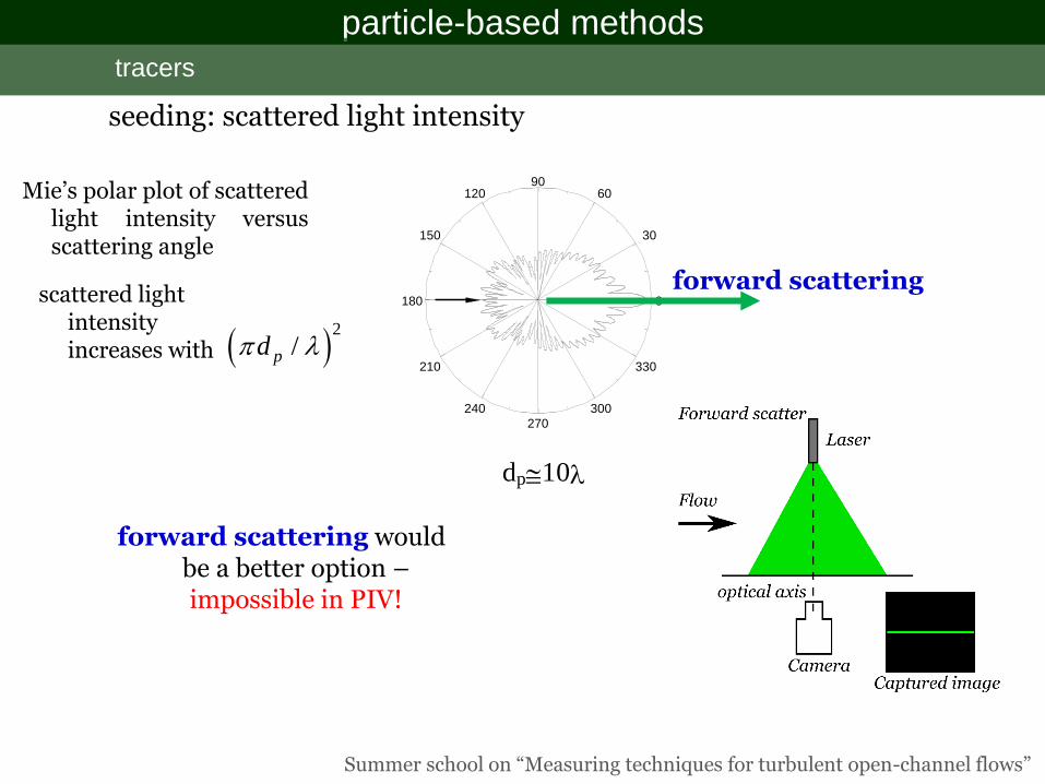
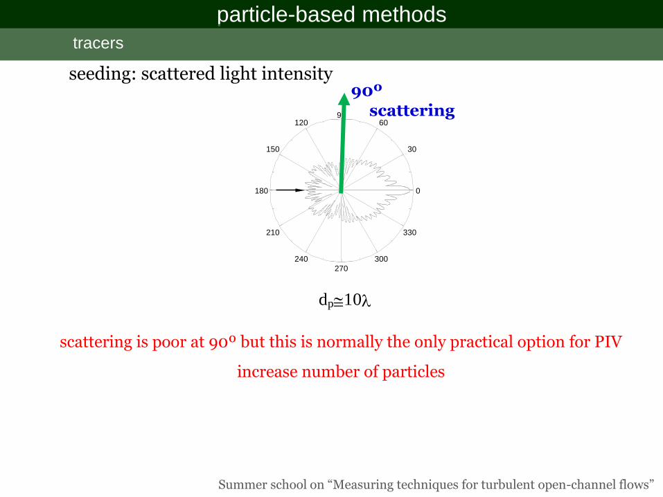
seeding: scattered light intensity
180 0
90
270
210
150
240
120
300
60
330
30
180 0
330210
240 300
270
150
120
90
60
30
180 0
210
150
240
120
270
9060
300
30
330
dp0.2 dp1.0 dp10
Mie’s polar plot of scattered light intensity versus scattering angle
scattered light intensity increases with
forward scattering would be a better option – impossible in PIV!
scattering is poor at 90º but this is normally the only practical option for PIV
increase number of particles
2
/pd
particle-based methods
tracers
Summer school on “Measuring techniques for turbulent open-channel flows”
seeding: scattered light intensity
180 0
210
150
240
120
270
9060
300
30
330
dp10
forward scattering would be a better option – impossible in PIV!
2
/pd
forward scattering
Mie’s polar plot of scattered light intensity versus scattering angle
scattered light intensity increases with
particle-based methods
tracers

Summer school on “Measuring techniques for turbulent open-channel flows”
seeding: scattered light intensity
180 0
210
150
240
120
270
9060
300
30
330
dp10
Mie’s polar plot of scattered light intensity versus scattering angle
scattered light intensity increases with
backward scattering would be another option – also difficult in PIV!
2
/pd
backward scattering
particle-based methods
tracers
Summer school on “Measuring techniques for turbulent open-channel flows”
seeding: scattered light intensity
180 0
210
150
240
120
270
9060
300
30
330
dp10
90º scattering
scattering is poor at 90º but this is normally the only practical option for PIV
increase number of particles
particle-based methods
tracers

Summer school on “Measuring techniques for turbulent open-channel flows”
PIV – pulse laser set up
How to see the tracers?
a PIV setup based on a pulsed laser
- laser head (laser production) - light sheet optics
digital camera (CCD, CMOS)
- frame grabber - timer control - acquisition software - preliminary data analysis
- timing unit (synchronization of laser and camera)
seeding particles
- power source
open “optical gates”
po
wer u
p la
se
r
power up laser user c
om
mands
op
en
sh
utte
r
store raw images processed data
external trigger

Summer school on “Measuring techniques for turbulent open-channel flows”
laser and light sheet optics
Laser (light amplification by stimulated emission of radiation)
- Laser material - pump source - resonator
Laser material - Helium-Neon, = 633 nm (red) (gas) – easy to produce, low power; - Argon-ion, = 514 nm (navy green) (gas) – difficult to pump, low efficiency, high power;
http://technology.niagarac.on.ca/people/mcsele/lasers/Lase
rsYag.htm
- Nd:YAG (neodymium-doped yttrium aluminium garnet), = 1064 nm (infrared), 532 nm (green) (solid state) – high power if operated with a “Quality switch” (Q-switch)
PIV – pulse laser set up
How to see the tracers?

Summer school on “Measuring techniques for turbulent open-channel flows”
laser and light sheet optics
Laser (light amplification by stimulated emission of radiation)
- Laser material - pump source - resonator
4 1E E E f Pump source pumping excites atoms to an upper energy level Laser light is produced by stimulated emission between two energy levels
pumping can be optical (white light for Nd:YAG), laser (diode lasers), or other electromagnetic
PIV – pulse laser set up
How to see the tracers?

Summer school on “Measuring techniques for turbulent open-channel flows”
laser and light sheet optics
Laser (light amplification by stimulated emission of radiation)
- Laser material - pump source - resonator
Resonator a resonator is achieved by mirror arrangement (the output mirror is partially reflecting)
the Q-switch (polarizer + Pokels cell) changes abruptly the resonance conditions; flash lamps operate and store energy but do not amplify light; that energy is released as a giant pulse when the Pokels cell removes polarization – an optical gate
PIV – pulse laser set up
How to see the tracers?

Summer school on “Measuring techniques for turbulent open-channel flows”
timing
Lasing threshold, pockles ON
Flashlamp Output
Energy in Nd:YAG
Enable Q-switch,
Laser Output Energy
Lasing threshold, pockles OFF
Ken Krieger
PIV – pulse laser set up
How to see the tracers?

Summer school on “Measuring techniques for turbulent open-channel flows”
laser and light sheet optics
Laser (light amplification by stimulated emission of radiation)
typical configuration
-Nd:YAG , optical pumping -double pulsed – Q-switch operated; - production at infrared 1024 nm - phase matching (while converting infrared 1064 nm to green 532 nm) - cooling system!
PIV – pulse laser set up
How to see the tracers?

Summer school on “Measuring techniques for turbulent open-channel flows”
laser and light sheet optics
Laser (light amplification by stimulated emission of radiation)
laser beam - modes of resonance transverse electric mode TEM
TEM00 is standard for Nd:Yag lasers
http://www.rp-photonics.com/beam_profilers.html
PIV – pulse laser set up
How to see the tracers?

Summer school on “Measuring techniques for turbulent open-channel flows”
laser and light sheet optics
Light sheet optics - telescope lenses; prismatic lenses;
- cylindrical lenses (production of laser sheet)
- mirrors, reflectors and -shutters
PIV – pulse laser set up
How to see the tracers?

Summer school on “Measuring techniques for turbulent open-channel flows”
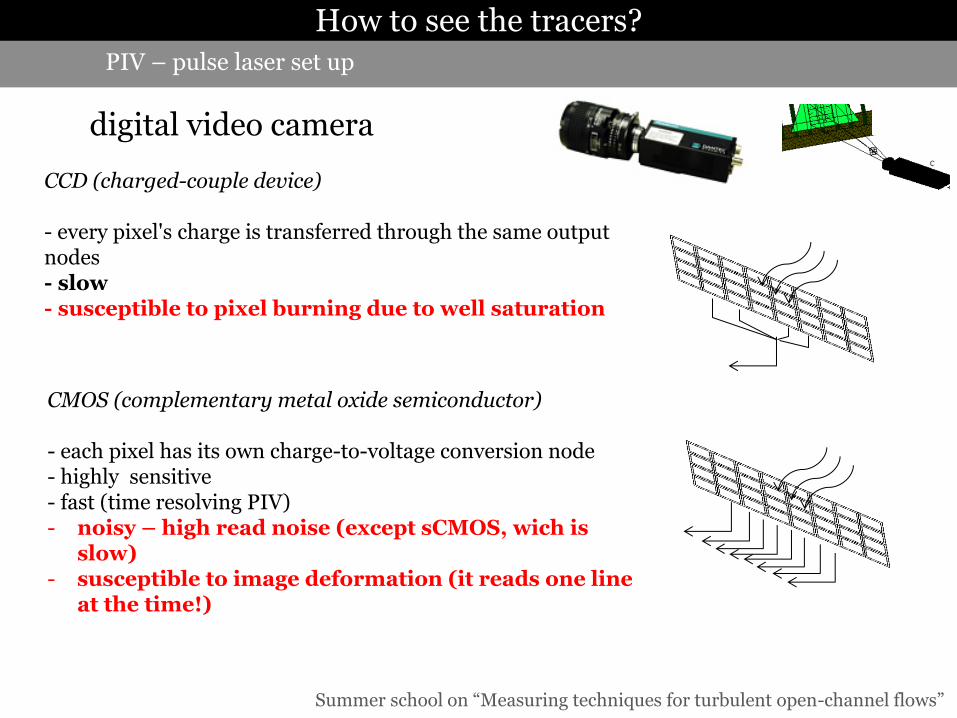
digital video camera
photoelectric effect
incoming photons
outgoing electrons
only sensitive to light intensity – ammount of energy, not wavelenght – no colour! (three cells per sensor to have colour, eg. RGB)
matrix of sensors (wells) with photosensitive cells
0
0
1 1eq V c
: electron charge, : stopping potential (volts); : Planck constant; : light velocity; :wave-length ; : threshold wavelength
(charge to voltage conversor)
eq0V
c
0
PIV – pulse laser set up
How to see the tracers?

Summer school on “Measuring techniques for turbulent open-channel flows”
digital video camera
pixel size (and focal length) - typical values: 10 um - minimize the ratio arc/pixel
dynamic range - the ratio of the maximum possible signal (full well capacity in electrons) and the noise signal (in the dark, rms electrons); eg: 15000/8 = 1875 ; 3750 steps 212 - requires 12 bit pixel depth pixel depth - number of shades resolved by the charge to voltage converter noise - photon noise (background noise, unavoidable) - thermal noise: electrons released by temperature (avoidable) - read noise: property of the electric circuits (controllable)
PIV – pulse laser set up
How to see the tracers?
Summer school on “Measuring techniques for turbulent open-channel flows”
digital video camera
CCD (charged-couple device) - every pixel's charge is transferred through the same output nodes - slow - susceptible to pixel burning due to well saturation
CMOS (complementary metal oxide semiconductor) - each pixel has its own charge-to-voltage conversion node - highly sensitive - fast (time resolving PIV) - noisy – high read noise (except sCMOS, wich is
slow) - susceptible to image deformation (it reads one line
at the time!)
PIV – pulse laser set up
How to see the tracers?

Summer school on “Measuring techniques for turbulent open-channel flows”
a PIV setup based on a continuous laser
- laser head (laser production) - light sheet optics
digital fast camera (CCD, CMOS)
- frame grabber - timer control - acquisition software - preliminary data analysis
seeding particles
- power source
po
wer u
p la
se
r
power up laser user c
om
mands
store raw images processed data
Advantages: cheaper laser, simpler electronics, dt< ms
Laser is continuous. Camera shutter defines the dt. Time resolved description
PIV – continuous laser set up
How to see the tracers?

Summer school on “Measuring techniques for turbulent open-channel flows”
a PIV/PTV setup without laser
Halogen projectors
LED projector
Mosaic of photos
PIV with no lasers
How to see the tracers?
Summer school on “Measuring techniques for turbulent open-channel flows”
PIV – spatial (eulerian) flow description
PTV – material (lagrangian) flow description or spatial flow description
PIV basics
How to see the tracers?
Summer school on “Measuring techniques for turbulent open-channel flows”
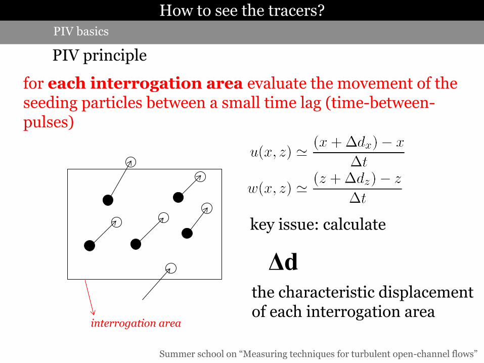
PIV principle
interrogation area
key issue: calculate
Δdthe characteristic displacement of each interrogation area
for each interrogation area evaluate the movement of the seeding particles between a small time lag (time-between-pulses)
PIV basics
How to see the tracers?

Summer school on “Measuring techniques for turbulent open-channel flows”
PIV principle
correlation of image pairs
Δdhow to calculate
clear peak ambiguous peak (low signal-to-noise ratio)
PIV basics
How to see the tracers?

Summer school on “Measuring techniques for turbulent open-channel flows”
PIV principle
Δdhow to calculate
Δd
it corresponds to the coordinates of the correlation peak in the referential of centre of the interrogation area
note that is not a mean displacement in the interrogation area! Δd
PIV basics
How to see the tracers?

Summer school on “Measuring techniques for turbulent open-channel flows”
PIV principle
- type of correlation (cross-correlation, adaptative)
-(relative) size of interrogation area/size of seeding particles - time-between-pulses
- number of seeding particles -use of windows/filters
- subpixel interpolation
parameters that control the quality of the correlation
PIV basics
How to see the tracers?

Summer school on “Measuring techniques for turbulent open-channel flows”
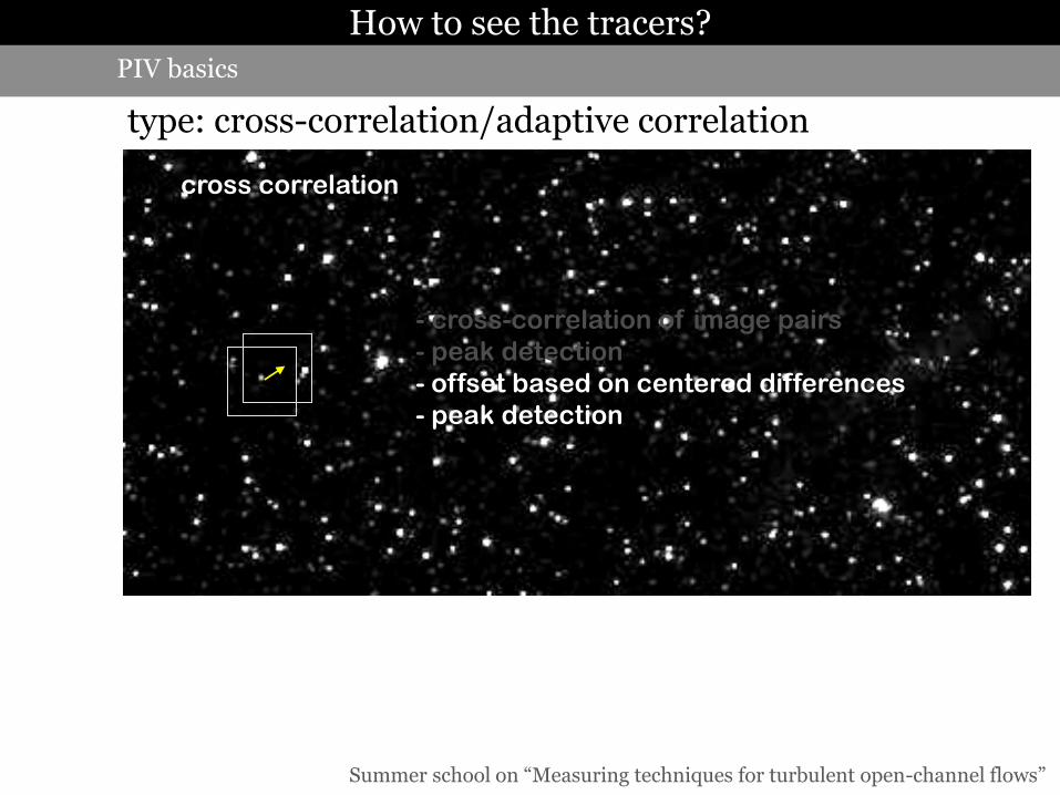
cross correlation
- cross-correlation of image pairs
- peak detection
PIV basics
How to see the tracers?
Summer school on “Measuring techniques for turbulent open-channel flows”
type: cross-correlation/adaptive correlation
cross correlation
- cross-correlation of image pairs
- peak detection
- offset based on centered differences
- peak detection
PIV basics
How to see the tracers?

Summer school on “Measuring techniques for turbulent open-channel flows”
adaptive correlation
- cross-correlation of image pairs
- peak detection
type: cross-correlation/adaptive correlation
PIV basics
How to see the tracers?

Summer school on “Measuring techniques for turbulent open-channel flows”
adaptive correlation
- cross-correlation of image pairs
- peak detection
- reduce size of interrogation area
- offset based on centered differences
- peak detection
- … (repeat)
type: cross-correlation/adaptive correlation
PIV basics
How to see the tracers?

Summer school on “Measuring techniques for turbulent open-channel flows”
Finding through good correlations
ideal: several non-overlapping particles moving 25% of the size of the interrogation area
Δd
- seed appropriately (a lot… 5 per final interrogation area);
- adjust size of the interrogation area relatively to the size of the particles – particles should be about 9 px2;
- adjust the time between pulses and the size of the interrogation area to meet the above ideal displacement.
(issues concerning time-between-pulses, size of seeding particles and number of seeding particles)
PIV basics
How to see the tracers?

Summer school on “Measuring techniques for turbulent open-channel flows”
Finding through good correlations Δd
be aware of out-of-plane loss of pairs (cause bias-to-zero) reduce time between pulses
in-plane loss of pairs consider windowing, consider offsetting
consider filtering to enhance peak width (may benefit subpixel
interpolation)
note that more than 50% movement causes aliasing! (Nyquist theorem) reduce time between pulses, increase interrogation area
PIV basics
How to see the tracers?
Summer school on “Measuring techniques for turbulent open-channel flows”
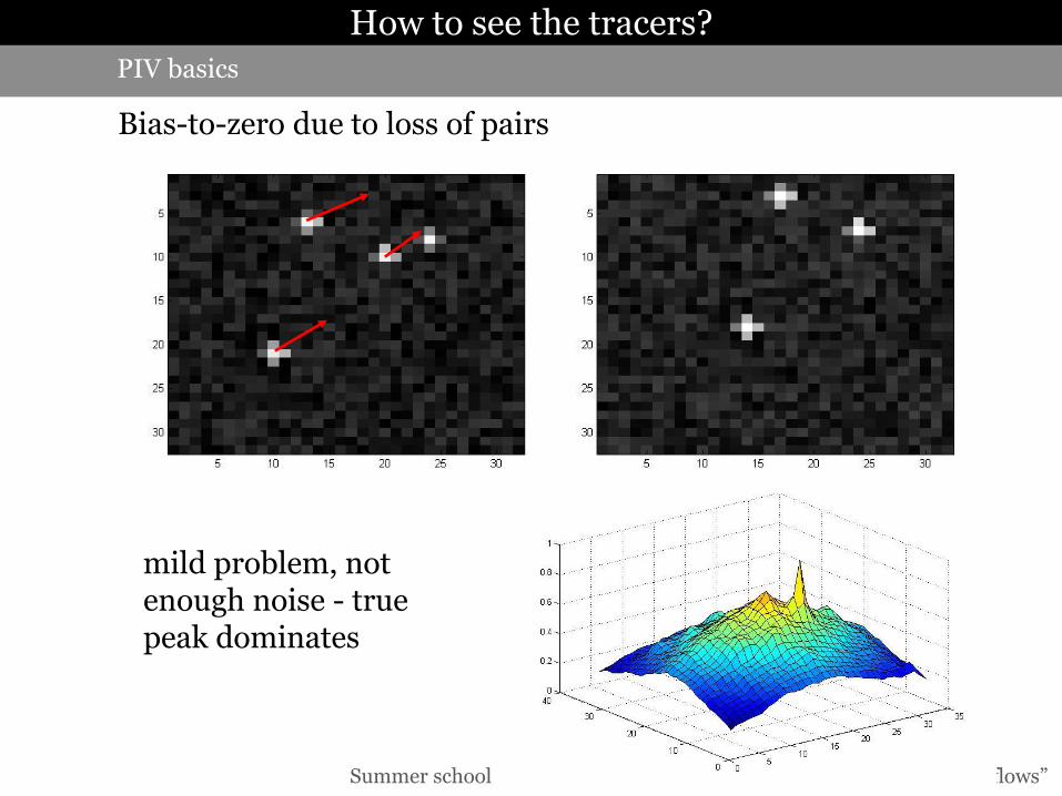
mild problem, not enough noise - true peak dominates
Bias-to-zero due to loss of pairs
PIV basics
How to see the tracers?
Summer school on “Measuring techniques for turbulent open-channel flows”
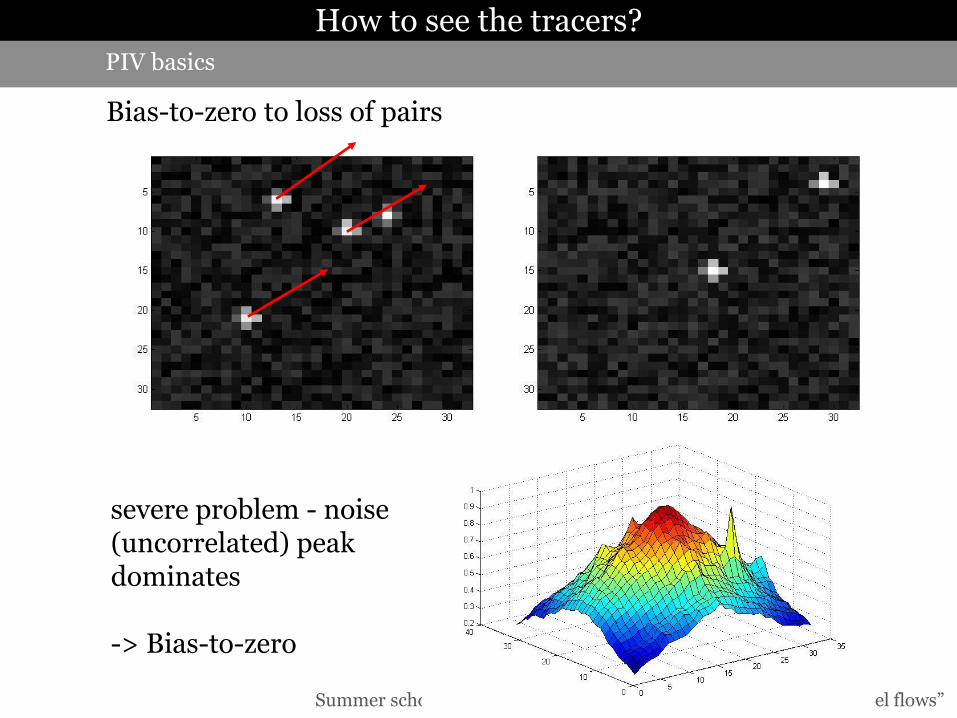
Noise dominates
severe problem - noise (uncorrelated) peak dominates -> Bias-to-zero
Bias-to-zero to loss of pairs
PIV basics
How to see the tracers?

Summer school on “Measuring techniques for turbulent open-channel flows”
Noise dominates
do not consider outer rim for correlation - true peak retrieved!
Windowing
PIV basics
How to see the tracers?

Summer school on “Measuring techniques for turbulent open-channel flows”
PTV basics
How to measure the tracers displacement?
PIV – spatial (eulerian) flow description
PTV – material (lagrangian) flow description or spatial flow description

Summer school on “Measuring techniques for turbulent open-channel flows”
Seeding concentration
http://www.piv.jp/data/01/piv01_1.bmp http://chemwiki.ucdavis.edu/@api/deki/f
iles/280/specklePattern.jpg
Laser Speckle PIV PTV
PTV basics
How to measure the tracers displacement?

Summer school on “Measuring techniques for turbulent open-channel flows”
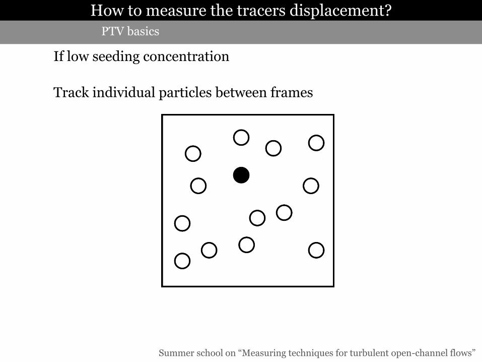
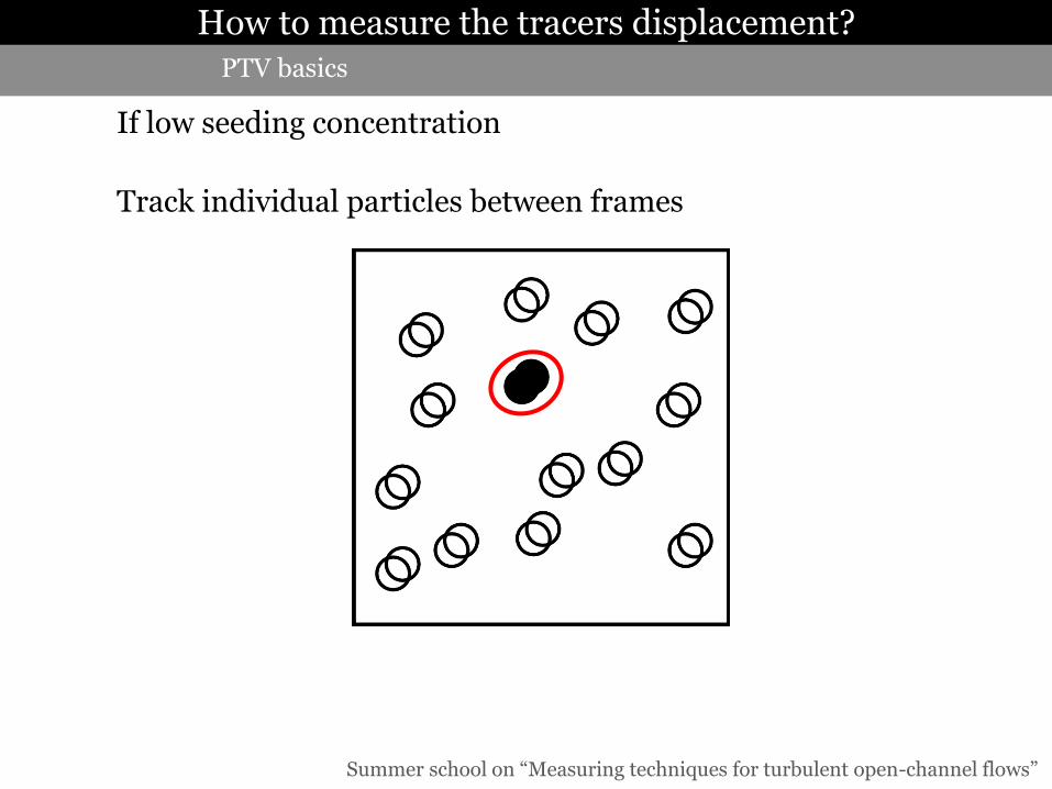
If low seeding concentration
Track individual particles between frames
PTV basics
How to measure the tracers displacement?
Summer school on “Measuring techniques for turbulent open-channel flows”
If low seeding concentration
Track individual particles between frames
PTV basics
How to measure the tracers displacement?

Summer school on “Measuring techniques for turbulent open-channel flows”
If low seeding concentration
Track individual particles between frames
PTV basics
How to measure the tracers displacement?
Summer school on “Measuring techniques for turbulent open-channel flows”
If low seeding concentration
Track individual particles between frames
PTV basics
How to measure the tracers displacement?

Summer school on “Measuring techniques for turbulent open-channel flows”
If low seeding concentration
Track individual particles between frames
Δd
PTV basics
How to measure the tracers displacement?

Summer school on “Measuring techniques for turbulent open-channel flows”
High computational cost a) particle-by-particle operation
Track individual particles between frames Contrary to PIV (based on image correlation) PTV does not have a base scheme. Many algorithms for PTV are based on different algorithms: Least displacement, Cluster methods, Probabilistic, Genetic algorithms, etc.
PTV basics
How to measure the tracers displacement?

Summer school on “Measuring techniques for turbulent open-channel flows”
be aware of / take in consideration that
Particle-based methods are not an non-intrusive measuring technique (can be extremely intrusive if Re is low and the fall velocity is large); PIV interrogation areas may smooth out small turbulent scales (be aware of anisotropy suppression); prone to noise (contrast, seeding, camera…) and to spikes (wrong correlation); data treatment is very time consuming.
Conclusions

Summer school on “Measuring techniques for turbulent open-channel flows”
be aware of / take in consideration that
PTV concentration is an issue many existing methods. detection of individual particles is critical data treatment is quite time consuming.
Conclusions

Summer school on “Measuring techniques for turbulent open-channel flows”
some references
[1] Wereley, S.T. & Meinhart, C.D. (2010). Recent Advances in Micro-Particle Image Velocimetry. Annual Review of Fluid Mechanics 42 (1): 557–576. doi:10.1146/annurev-fluid-121108-145427 [2] Raffel, M.; Willert, C.; Wereley, S. & Kompenhans, J. (2007) Particle Image Velocimetry, A Practical Guide, 2nd edn. Springer [3] Adrian, R.J. (2005). Twenty years of particle image velocimetry. Experiments in Fluids 39 (2): 159–169. doi:10.1007/s00348-005-0991-7 [4] Adrian, R. J. (1991) Particle imaging techniques for experimental fluid mechanics, Annual Review of Fluid Mechanics, vol.23, pp. 261-304. A lot more fundamental refs in [2]…
Conclusions

Summer school on “Measuring techniques for turbulent open-channel flows”
Yet another animation…
The end…
Thank you!
![Title On the state-of-the-art of particle methods for coastal ......4 method [Chorin, 1968]. Hence, they can be referred to as projection-based particle methods. Several comparative](https://img.pdfslide.us/doc/110x75/60cbe37968ffea482646717a/title-on-the-state-of-the-art-of-particle-methods-for-coastal-4-method-chorin.jpg)