1

Introduction to Parallel Computing

Yao-Yuan Chuang

2

Outline Overview Concepts and Terminology Parallel Computer Memory Architectures Parallel Programming Models Designing Parallel Programs Parallel Examples References

3

Overview What is Parallel Computing? Why use Parallel Computing?

4

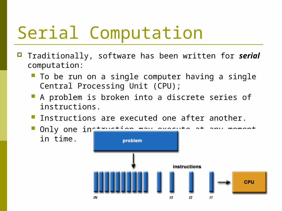
Serial Computation Traditionally, software has been written for serial

computation: To be run on a single computer having a single Central

Processing Unit (CPU); A problem is broken into a discrete series of instructions. Instructions are executed one after another. Only one instruction may execute at any moment in

time.

5

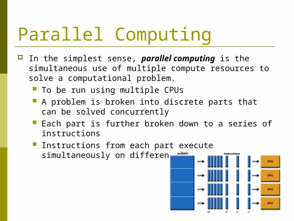
Parallel Computing In the simplest sense, parallel computing is the

simultaneous use of multiple compute resources to solve a computational problem. To be run using multiple CPUs A problem is broken into discrete parts that can be

solved concurrently Each part is further broken down to a series of

instructions Instructions from each part execute simultaneously on

different CPUs

6

Resource and Problem The compute resources can include:

A single computer with multiple processors; An arbitrary number of computers connected by a

network; A combination of both.

The computational problem usually demonstrates characteristics such as the ability to be: Broken apart into discrete pieces of work that can be

solved simultaneously; Execute multiple program instructions at any moment in

time; Solved in less time with multiple compute resources

than with a single compute resource.

7

Grand Challenge Problems Traditionally, parallel computing has been considered to be

"the high end of computing" and has been motivated by numerical simulations of complex systems and "Grand Challenge Problems" such as:

weather and climate chemical and nuclear reactions biological, human genome geological, seismic activity mechanical devices - from prosthetics to spacecraft electronic circuits manufacturing processes

8

Applications Today, commercial applications are providing an equal or

greater driving force in the development of faster computers. These applications require the processing of large amounts of data in sophisticated ways. Example applications include: parallel databases, data mining oil exploration web search engines, web based business services computer-aided diagnosis in medicine management of national and multi-national corporations advanced graphics and virtual reality, particularly in the

entertainment industry networked video and multi-media technologies collaborative work environments

Ultimately, parallel computing is an attempt to maximize the infinite but seemingly scarce commodity called time.

9

Why use parallel computing? The primary reasons for using parallel computing:

Save time - wall clock time Solve larger problems Provide concurrency (do multiple things at the same time)

Other reasons might include: Taking advantage of non-local resources - using available

compute resources on a wide area network, or even the Internet when local compute resources are scarce.

Cost savings - using multiple "cheap" computing resources instead of paying for time on a supercomputer.

Overcoming memory constraints - single computers have very finite memory resources. For large problems, using the memories of multiple computers may overcome this obstacle.

10

Why use parallel computing? Limits to serial computing - both physical and practical reasons pose

significant constraints to simply building ever faster serial computers: Transmission speeds - the speed of a serial computer is directly

dependent upon how fast data can move through hardware. Absolute limits are the speed of light (30 cm/nanosecond) and the transmission limit of copper wire (9 cm/nanosecond). Increasing speeds necessitate increasing proximity of processing elements.

Limits to miniaturization - processor technology is allowing an increasing number of transistors to be placed on a chip. However, even with molecular or atomic-level components, a limit will be reached on how small components can be.

Economic limitations - it is increasingly expensive to make a single processor faster. Using a larger number of moderately fast commodity processors to achieve the same (or better) performance is less expensive.

The future: during the past 10 years, the trends indicated by ever faster networks, distributed systems, and multi-processor computer architectures (even at the desktop level) suggest that parallelism is the future of computing.

11

Concept and Terminology Von Newmann Architecture Flynn’s Classical Taxonomy Parallel Terminology

12

Von Neumann Architecture For over 40 years, virtually all computers have followed a

common machine model known as the von Neumann computer. Named after the Hungarian mathematician John von Neumann.

A von Neumann computer uses the stored-program concept. The CPU executes a stored program that specifies a sequence of read and write operations on the memory.

Basic design: Memory is used to store both program and data

instructions Program instructions are coded data which tell the

computer to do something Data is simply information to be used by the program A central processing unit (CPU) gets instructions and/or

data from memory, decodes the instructions and then sequentially performs them.

13

Flynn’s Classical Taxonomy There are different ways to classify parallel computers. One

of the more widely used classifications, in use since 1966, is called Flynn's Taxonomy.

Flynn's taxonomy distinguishes multi-processor computer architectures according to how they can be classified along the two independent dimensions of Instruction and Data. Each of these dimensions can have only one of two possible states: Single or Multiple.

There are 4 possible classifications according to Flynn. Single Instruction, Single Data (SISD) Single Instruction, Multiple Data (SIMD) Multiple Instruction, Single Data (MISD) Multiple Instruction, Multiple Data (MIMD)

14

Single Instruction Single Data A serial (non-parallel) computer Single instruction: only one instruction

stream is being acted on by the CPU during any one clock cycle

Single data: only one data stream is being used as input during any one clock cycle

Deterministic execution This is the oldest and until recently, the

most prevalent form of computer Examples: most PCs, single CPU

workstations and mainframes

15

Single Instruction Multiple Data A type of parallel computer Single instruction: All processing units execut

e the same instruction at any given clock cycle

Multiple data: Each processing unit can operate on a different data element

This type of machine typically has an instruction dispatcher, a very high-bandwidth internal network, and a very large array of very small-capacity instruction units.

Best suited for specialized problems characterized by a high degree of regularity,such as image processing.

Synchronous (lockstep) and deterministic execution

Two varieties: Processor Arrays and Vector Pipelines

Examples: Processor Arrays: Connection Machine C

M-2, Maspar MP-1, MP-2 Vector Pipelines: IBM 9000, Cray C90, Fujit

su VP, NEC SX-2, Hitachi S820

16

Multiple Instruction Single Data

A single data stream is fed into multiple processing units.

Each processing unit operates on the data independently via independent instruction streams.

Few actual examples of this class of parallel computer have ever existed. One is the experimental Carnegie-Mellon C.mmp computer (1971).

Some conceivable uses might be: multiple frequency filters operating

on a single signal stream multiple cryptography algorithms att

empting to crack a single coded message.

17

Multiple Instruction Multiple Data

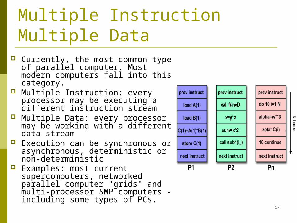
Currently, the most common type of parallel computer. Most modern computers fall into this category.

Multiple Instruction: every processor may be executing a different instruction stream

Multiple Data: every processor may be working with a different data stream

Execution can be synchronous or asynchronous, deterministic or non-deterministic

Examples: most current supercomputers, networked parallel computer "grids" and multi-processor SMP computers - including some types of PCs.

18

Parallel Terminology Task

A logically discrete section of computational work. A task is typically a program or program-like set of instructions that is executed by a processor.

Parallel Task A task that can be executed by multiple processors safely (yields

correct results)

Serial Execution Execution of a program sequentially, one statement at a time. In the

simplest sense, this is what happens on a one processor machine. However, virtually all parallel tasks will have sections of a parallel program that must be executed serially.

Parallel Execution Execution of a program by more than one task, with each task being

able to execute the same or different statement at the same moment in time.

19

Parallel Terminology Shared Memory

From a strictly hardware point of view, describes a computer architecture where all processors have direct (usually bus based) access to common physical memory. In a programming sense, it describes a model where parallel tasks all have the same "picture" of memory and can directly address and access the same logical memory locations regardless of where the physical memory actually exists.

Distributed Memory In hardware, refers to network based memory access for physical

memory that is not common. As a programming model, tasks can only logically "see" local machine memory and must use communications to access memory on other machines where other tasks are executing.

Communications Parallel tasks typically need to exchange data. There are several ways

this can be accomplished, such as through a shared memory bus or over a network, however the actual event of data exchange is commonly referred to as communications regardless of the method employed.

20

Parallel Terminology Synchronization

The coordination of parallel tasks in real time, very often associated with communications. Often implemented by establishing a synchronization point within an application where a task may not proceed further until another task(s) reaches the same or logically equivalent point. Synchronization usually involves waiting by at least one task, and can therefore cause a parallel application's wall clock execution time to increase.

Granularity In parallel computing, granularity is a qualitative measure of the ratio of com

putation to communication. Coarse: relatively large amounts of computational work are done between commu

nication events Fine: relatively small amounts of computational work are done between communi

cation events Observed Speedup

Observed speedup of a code which has been parallelized, defined as: wall-clock time of serial execution / wall-clock time of parallel execution

One of the simplest and most widely used indicators for a parallel program's performance.

21

Parallel Terminology Parallel Overhead

The amount of time required to coordinate parallel tasks, as opposed to doing useful work. Parallel overhead can include factors such as:

Task start-up time Synchronizations Data communications Software overhead imposed by parallel compilers, libraries, tools, operating s

ystem, etc. Task termination time

Massively Parallel Refers to the hardware that comprises a given parallel system - having many

processors. The meaning of many keeps increasing, but currently BG/L pushes this number to 6 digits.

Scalability Refers to a parallel system's (hardware and/or software) ability to demonstra

te a proportionate increase in parallel speedup with the addition of more processors. Factors that contribute to scalability include:

Hardware - particularly memory-cpu bandwidths and network communications

Application algorithm Parallel overhead related Characteristics of your specific application and coding

22

Parallel Computer Memory Architectures Shared Memory Distributed Memory Hybrid Distributed Shared Memory

23

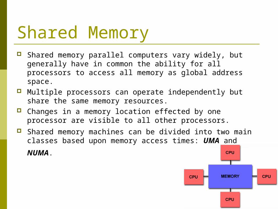
Shared Memory Shared memory parallel computers vary widely, but generally

have in common the ability for all processors to access all memory as global address space.

Multiple processors can operate independently but share the same memory resources.

Changes in a memory location effected by one processor are visible to all other processors.

Shared memory machines can be divided into two main classes

based upon memory access times: UMA and NUMA.

24

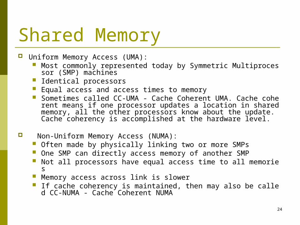
Shared Memory Uniform Memory Access (UMA):

Most commonly represented today by Symmetric Multiprocessor (SMP) machines

Identical processors Equal access and access times to memory Sometimes called CC-UMA - Cache Coherent UMA. Cache coherent m

eans if one processor updates a location in shared memory, all the other processors know about the update. Cache coherency is accomplished at the hardware level.

Non-Uniform Memory Access (NUMA): Often made by physically linking two or more SMPs One SMP can directly access memory of another SMP Not all processors have equal access time to all memories Memory access across link is slower If cache coherency is maintained, then may also be called CC-NUMA

- Cache Coherent NUMA

25

Shared Memory Advantages:

Global address space provides a user-friendly programming perspective to memory

Data sharing between tasks is both fast and uniform due to the proximity of memory to CPUs

Disadvantages: Primary disadvantage is the lack of scalability between

memory and CPUs. Adding more CPUs can geometrically increases traffic on the shared memory-CPU path, and for cache coherent systems, geometrically increase traffic associated with cache/memory management.

Programmer responsibility for synchronization constructs that insure "correct" access of global memory.

Expense: it becomes increasingly difficult and expensive to design and produce shared memory machines with ever increasing numbers of processors.

26

Distributed Memory Like shared memory systems, distributed memory systems vary

widely but share a common characteristic. Distributed memory systems require a communication network to connect inter-processor memory.

Processors have their own local memory. Memory addresses in one processor do not map to another processor, so there is no concept of global address space across all processors.

Because each processor has its own local memory, it operates independently. Changes it makes to its local memory have no effect on the memory of other processors. Hence, the concept of cache coherency does not apply.

When a processor needs access to data in another processor, it is usually the task of the programmer to explicitly define how and when data is communicated. Synchronization between tasks is likewise the programmer's responsibility.

The network "fabric" used for data transfer varies widely, though it can can be as simple as Ethernet.

27

Distributed Memory Advantages:

Memory is scalable with number of processors. Increase the number of processors and the size of memory increases proportionately.

Each processor can rapidly access its own memory without interference and without the overhead incurred with trying to maintain cache coherency.

Cost effectiveness: can use commodity, off-the-shelf processors and networking.

Disadvantages: The programmer is responsible for many of the details associ

ated with data communication between processors. It may be difficult to map existing data structures, based on gl

obal memory, to this memory organization. Non-uniform memory access (NUMA) times

28

Distributed Shared Memory The largest and fastest computers in the world today employ both s

hared and distributed memory architectures. The shared memory component is usually a cache coherent SMP ma

chine. Processors on a given SMP can address that machine's memory as global.

The distributed memory component is the networking of multiple SMPs. SMPs know only about their own memory - not the memory on another SMP. Therefore, network communications are required to move data from one SMP to another.

Current trends seem to indicate that this type of memory architecture will continue to prevail and increase at the high end of computing for the foreseeable future.

Advantages and Disadvantages: whatever is common to both shared and distributed memory architectures.

29

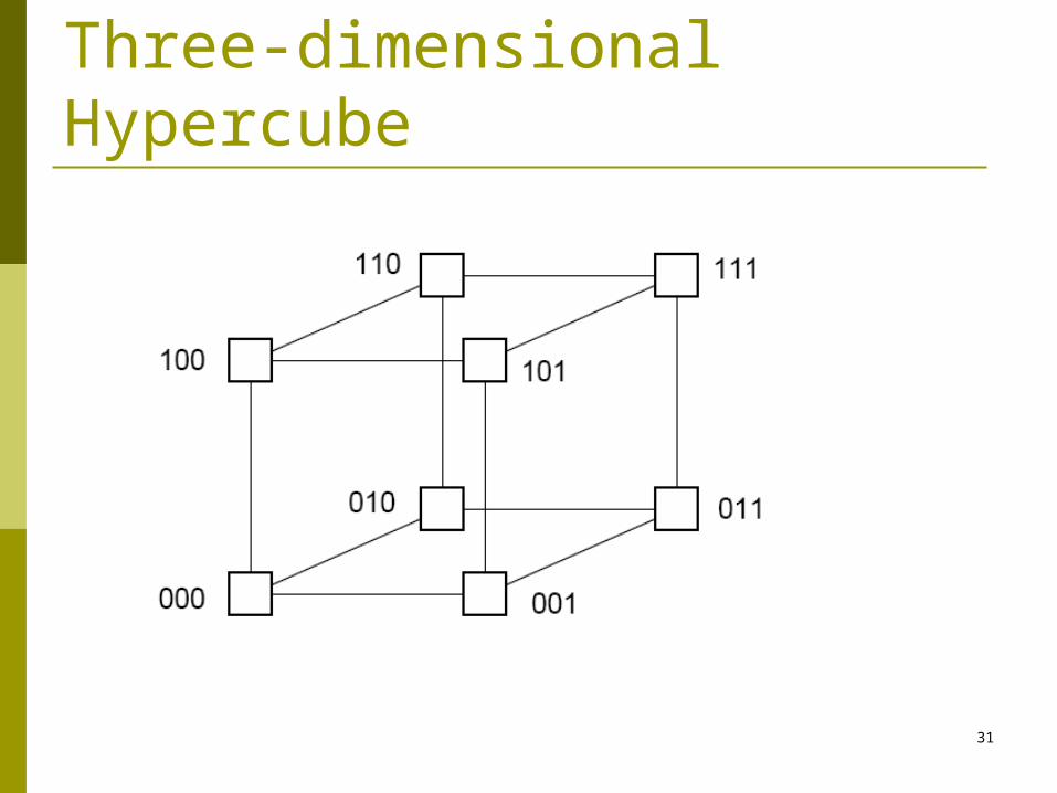
Interconnection Network With direct links between computers

Exhausive connections 2D and 3D meshs Hypercube

Using Switches Crossbar Trees Multistage interconnection network

30

Two Dimensional Array

31

Three-dimensional Hypercube

32

Four-dimensional hypercube

Hypercubes popular in 1980’s not now

33

Crossbar switch

34

Tree

35

Multistage Interconnection Network

36

Parallel Programming Model There are several parallel programming models in common use:

Shared Memory Threads Message Passing Data Parallel Hybrid

Parallel programming models exist as an abstraction above hardware and memory architectures.

Although it might not seem apparent, these models are NOT specific to a particular type of machine or memory architecture. In fact, any of these models can (theoretically) be implemented on any underlying hardware.

Which model to use is often a combination of what is available and personal choice. There is no "best" model, although there certainly are better implementations of some models over others.

The following sections describe each of the models mentioned above, and also discuss some of their actual implementations.

37

Shared Memory Model In the shared-memory programming model, tasks share a common address

space, which they read and write asynchronously. Various mechanisms such as locks / semaphores may be used to control

access to the shared memory. An advantage of this model from the programmer's point of view is that

the notion of data "ownership" is lacking, so there is no need to specify explicitly the communication of data between tasks. Program development can often be simplified.

An important disadvantage in terms of performance is that it becomes more difficult to understand and manage data locality.

Implementations: On shared memory platforms, the native compilers translate user program

variables into actual memory addresses, which are global. No common distributed memory platform implementations currently exist.

However, as mentioned previously in the Overview section, the KSR ALLCACHE approach provided a shared memory view of data even though the physical memory of the machine was distributed.

38

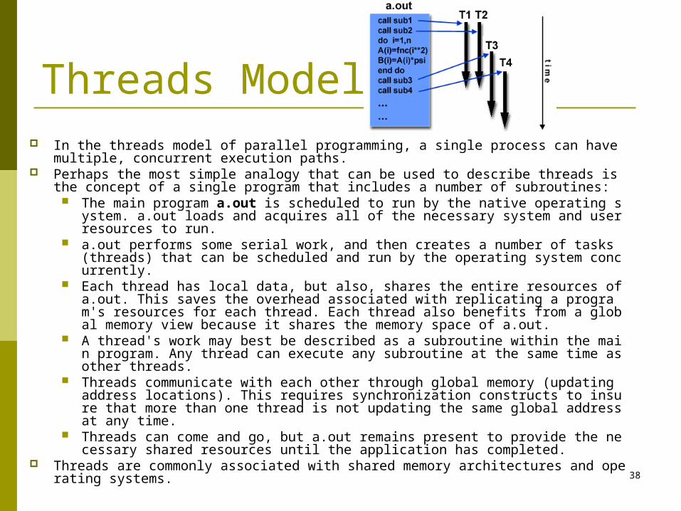
Threads Model In the threads model of parallel programming, a single process can have multiple, con

current execution paths. Perhaps the most simple analogy that can be used to describe threads is the concept o

f a single program that includes a number of subroutines: The main program a.out is scheduled to run by the native operating system. a.out

loads and acquires all of the necessary system and user resources to run. a.out performs some serial work, and then creates a number of tasks (threads) tha

t can be scheduled and run by the operating system concurrently. Each thread has local data, but also, shares the entire resources of a.out. This save

s the overhead associated with replicating a program's resources for each thread. Each thread also benefits from a global memory view because it shares the memory space of a.out.

A thread's work may best be described as a subroutine within the main program. Any thread can execute any subroutine at the same time as other threads.

Threads communicate with each other through global memory (updating address locations). This requires synchronization constructs to insure that more than one thread is not updating the same global address at any time.

Threads can come and go, but a.out remains present to provide the necessary shared resources until the application has completed.

Threads are commonly associated with shared memory architectures and operating systems.

39

Threads Model POSIX Threads

Library based; requires parallel coding Specified by the IEEE POSIX 1003.1c standard (1995). C Language only Commonly referred to as Pthreads. Most hardware vendors now offer Pthreads in addition to their proprietary t

hreads implementations. Very explicit parallelism; requires significant programmer attention to detail.

OpenMP

Compiler directive based; can use serial code Jointly defined and endorsed by a group of major computer hardware and s

oftware vendors. The OpenMP Fortran API was released October 28, 1997. The C/C++ API was released in late 1998.

Portable / multi-platform, including Unix and Windows NT platforms Available in C/C++ and Fortran implementations Can be very easy and simple to use - provides for "incremental parallelism“

Microsoft has its own implementation for threads, which is not related to the UNIX POSIX standard or OpenMP.

40

Message Passing Model The message passing model demonstrates the following

characteristics: A set of tasks that use their own local memory during

computation. Multiple tasks can reside on the same physical machine as well across an arbitrary number of machines.

Tasks exchange data through communications by sending and receiving messages.

Data transfer usually requires cooperative operations to be performed by each process. For example, a send operation must have a matching receive operation.

41

Message Passing Model From a programming perspective, message passing implementations comm

only comprise a library of subroutines that are imbedded in source code. The programmer is responsible for determining all parallelism.

Historically, a variety of message passing libraries have been available since the 1980s. These implementations differed substantially from each other making it difficult for programmers to develop portable applications.

In 1992, the MPI Forum was formed with the primary goal of establishing a standard interface for message passing implementations.

Part 1 of the Message Passing Interface (MPI) was released in 1994. Part 2 (MPI-2) was released in 1996. Both MPI specifications are available on the web at www.mcs.anl.gov/Projects/mpi/standard.html.

MPI is now the "de facto" industry standard for message passing, replacing virtually all other message passing implementations used for production work. Most, if not all of the popular parallel computing platforms offer at least one implementation of MPI. A few offer a full implementation of MPI-2.

For shared memory architectures, MPI implementations usually don't use a network for task communications. Instead, they use shared memory (memory copies) for performance reasons.

MPICH2 and OPENMPI are new implementation of MPI-2.

42

Data Parallel Model he data parallel model demonstrates the

following characteristics: Most of the parallel work focuses on

performing operations on a data set. The data set is typically organized into a common structure, such as an array or cube.

A set of tasks work collectively on the same data structure, however, each task works on a different partition of the same data structure.

Tasks perform the same operation on their partition of work, for example, "add 4 to every array element".

On shared memory architectures, all tasks may have access to the data structure through global memory. On distributed memory architectures the data structure is split up and resides as "chunks" in the local memory of each task.

43

Data Parallel Model Fortran 90 and 95 (F90, F95): ISO/ANSI standard extensions to Fortran 77.

Contains everything that is in Fortran 77 New source code format; additions to character set Additions to program structure and commands Variable additions - methods and arguments Pointers and dynamic memory allocation added Array processing (arrays treated as objects) added Recursive and new intrinsic functions added Many other new features Implementations are available for most common parallel platforms.

High Performance Fortran (HPF): Extensions to Fortran 90 to support data parallel programming. Contains everything in Fortran 90 Directives to tell compiler how to distribute data added Assertions that can improve optimization of generated code added Data parallel constructs added (now part of Fortran 95) Implementations are available for most common parallel platforms.

Compiler Directives

44

Parallel Programming Model Other parallel programming models besides those

previously mentioned certainly exist, and will continue to evolve along with the ever changing world of computer hardware and software. Only three of the more common ones are mentioned here. Hybrid Single Program Multiple Data (SPMD) Multiple Program Multiple Data (MPMD)

45

Hybrid In this model, any two or more parallel programming models are

combined. Currently, a common example of a hybrid model is the combinati

on of the message passing model (MPI) with either the threads model (POSIX threads) or the shared memory model (OpenMP). This hybrid model lends itself well to the increasingly common hardware environment of networked SMP machines.

Another common example of a hybrid model is combining data parallel with message passing. As mentioned in the data parallel model section previously, data parallel implementations (F90, HPF) on distributed memory architectures actually use message passing to transmit data between tasks, transparently to the programmer.

46

Single Program Multiple Data SPMD is actually a "high level" programming model that

can be built upon any combination of the previously mentioned parallel programming models.

A single program is executed by all tasks simultaneously. At any moment in time, tasks can be executing the same or

different instructions within the same program. SPMD programs usually have the necessary logic

programmed into them to allow different tasks to branch or conditionally execute only those parts of the program they are designed to execute. That is, tasks do not necessarily have to execute the entire program - perhaps only a portion of it.

All tasks may use different data

47

Multiple Program Multiple Data Like SPMD, MPMD is actually a "high level" programming

model that can be built upon any combination of the previously mentioned parallel programming models.

MPMD applications typically have multiple executable object files (programs). While the application is being run in parallel, each task can be executing the same or different program as other tasks.

All tasks may use different data

48

Automatic vs. Manual Parallelization A parallelizing compiler generally works in two different ways: Fully Automatic

The compiler analyzes the source code and identifies opportunities for parallelism.

The analysis includes identifying inhibitors to parallelism and possibly a cost weighting on whether or not the parallelism would actually improve performance.

Loops (do, for) loops are the most frequent target for automatic parallelization.

Programmer Directed Using "compiler directives" or possibly compiler flags, the

programmer explicitly tells the compiler how to parallelize the code.

May be able to be used in conjunction with some degree of automatic parallelization also.

49

Automatic vs. Manual Parallelization Designing and developing parallel programs has

characteristically been a very manual process. The programmer is typically responsible for both identifying and actually implementing parallelism.

Very often, manually developing parallel codes is a time consuming, complex, error-prone and iterative process.

If you are beginning with an existing serial code and have time or budget constraints, then automatic parallelization may be the answer. However, there are several important caveats that apply to automatic parallelization: Wrong results may be produced Performance may actually degrade Much less flexible than manual parallelization Limited to a subset (mostly loops) of code May actually not parallelize code if the analysis suggests there

are inhibitors or the code is too complex Most automatic parallelization tools are for Fortran

The remainder of this section applies to the manual method of developing parallel codes.

50

Design Parallel Program Understand the problem and the program Partitioning Communications Synchronization Data Dependencies Load Balancing Granularity I/O Limits and Costs of Parallel Programming Performance Analysis and Tuning

51

Understand problem Undoubtedly, the first step in developing parallel software is to first

understand the problem that you wish to solve in parallel. If you are starting with a serial program, this necessitates understanding the existing code also.

Before spending time in an attempt to develop a parallel solution for a problem, determine whether or not the problem is one that can actually be parallelized.

Identify the program's hotspots: Know where most of the real work is being done. The majority of scientific and

technical programs usually accomplish most of their work in a few places. Profilers and performance analysis tools can help here Focus on parallelizing the hotspots and ignore those sections of the program that

account for little CPU usage. Identify bottlenecks in the program

Are there areas that are disproportionately slow, or cause parallelizable work to halt or be deferred? For example, I/O is usually something that slows a program down.

May be possible to restructure the program or use a different algorithm to reduce or eliminate unnecessary slow areas

Identify inhibitors to parallelism. One common class of inhibitor is data dependence, as demonstrated by the Fibonacci sequence above.

Investigate other algorithms if possible. This may be the single most important consideration when designing a parallel application.

52

Partitioning One of the first steps in designing a parallel program is

to break the problem into discrete "chunks" of work that can be distributed to multiple tasks. This is known as decomposition or partitioning.

There are two basic ways to partition computational work among parallel tasks: domain decomposition and functional decomposition.

53

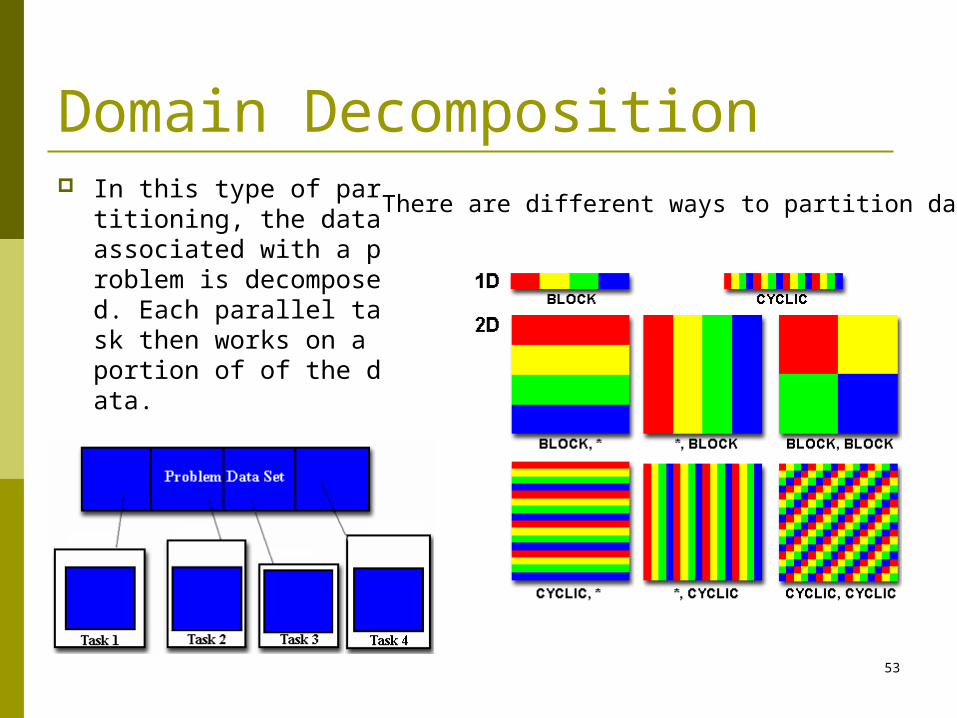
Domain Decomposition In this type of partitioni

ng, the data associated with a problem is decomposed. Each parallel task then works on a portion of of the data.

There are different ways to partition data:

54

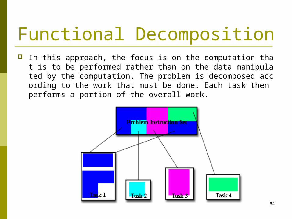
Functional Decomposition In this approach, the focus is on the computation that is to be perfor

med rather than on the data manipulated by the computation. The problem is decomposed according to the work that must be done. Each task then performs a portion of the overall work.

55

Communications You DON'T need communications

Some types of problems can be decomposed and executed in parallel with virtually no need for tasks to share data. For example, imagine an image processing operation where every pixel in a black and white image needs to have its color reversed. The image data can easily be distributed to multiple tasks that then act independently of each other to do their portion of the work.

These types of problems are often called embarrassingly parallel because they are so straight-forward. Very little inter-task communication is required.

You DO need communications

Most parallel applications are not quite so simple, and do require tasks to share data with each other. For example, a 3-D heat diffusion problem requires a task to know the temperatures calculated by the tasks that have neighboring data. Changes to neighboring data has a direct effect on that task's data.

56

Communications - factors Cost of communications

Inter-task communication virtually always implies overhead. Machine cycles and resources that could be used for

computation are instead used to package and transmit data. Communications frequently require some type of

synchronization between tasks, which can result in tasks spending time "waiting" instead of doing work.

Competing communication traffic can saturate the available network bandwidth, further aggravating performance problems.

Latency vs. Bandwidth latency is the time it takes to send a minimal (0 byte)

message from point A to point B. Commonly expressed as microseconds.

bandwidth is the amount of data that can be communicated per unit of time. Commonly expressed as megabytes/sec.

Sending many small messages can cause latency to dominate communication overheads. Often it is more efficient to package small messages into a larger message, thus increasing the effective communications bandwidth.

57

Communications Visibility of communications

With the Message Passing Model, communications are explicit and generally quite visible and under the control of the programmer.

With the Data Parallel Model, communications often occur transparently to the programmer, particularly on distributed memory architectures. The programmer may not even be able to know exactly how inter-task communications are being accomplished.

Synchronous vs. asynchronous communications Synchronous communications require some type of "handshaking" between

tasks that are sharing data. This can be explicitly structured in code by the programmer, or it may happen at a lower level unknown to the programmer.

Synchronous communications are often referred to as blocking communications since other work must wait until the communications have completed.

Asynchronous communications allow tasks to transfer data independently from one another. For example, task 1 can prepare and send a message to task 2, and then immediately begin doing other work. When task 2 actually receives the data doesn't matter.

Asynchronous communications are often referred to as non-blocking communications since other work can be done while the communications are taking place.

Interleaving computation with communication is the single greatest benefit for using asynchronous communications.

58

Communications Scope of communications

Knowing which tasks must communicate with each other is critical during the design stage of a parallel code. Both of the two scopings described below can be implemented synchronously or asynchronously.

Point-to-point - involves two tasks with one task acting as the sender/producer of data, and the other acting as the receiver/consumer.

Collective - involves data sharing between more than two tasks, which are often specified as being members in a common group, or collective. Some common variations (there are more):

59

Communications Efficiency of communications

Very often, the programmer will have a choice with regard to factors that can affect communications performance. Only a few are mentioned here.

Which implementation for a given model should be used? Using the Message Passing Model as an example, one MPI implementation may be faster on a given hardware platform than another.

What type of communication operations should be used? As mentioned previously, asynchronous communication operations can improve overall program performance.

Network media - some platforms may offer more than one network for communications. Which one is best?

60

Synchronization Barrier

Usually implies that all tasks are involved Each task performs its work until it reaches the barrier. It then stops,

or "blocks". When the last task reaches the barrier, all tasks are synchronized. What happens from here varies. Often, a serial section of work must

be done. In other cases, the tasks are automatically released to continue their work.

Lock / semaphore Can involve any number of tasks Typically used to serialize (protect) access to global data or a

section of code. Only one task at a time may use (own) the lock / semaphore / flag.

The first task to acquire the lock "sets" it. This task can then safely (serially) access the protected data or code.

Other tasks can attempt to acquire the lock but must wait until the task that owns the lock releases it.

Can be blocking or non-blocking

61

Synchronization Synchronous communication operations

Involves only those tasks executing a communication operation

When a task performs a communication operation, some form of coordination is required with the other task(s) participating in the communication. For example, before a task can perform a send operation, it must first receive an acknowledgment from the receiving task that it is OK to send.

Discussed previously in the Communications section.

62

Data Dependencies A dependence exists between program statements when the ord

er of statement execution affects the results of the program. A data dependence results from multiple use of the same locati

on(s) in storage by different tasks. Dependencies are important to parallel programming because th

ey are one of the primary inhibitors to parallelism. Examples:

Loop carried data dependence Loop independent data dependence

How to Handle Data Dependencies: Distributed memory architectures - communicate required da

ta at synchronization points. Shared memory architectures -synchronize read/write operat

ions between tasks.

63

Load Balancing Load balancing refers to the practice of distributing work

among tasks so that all tasks are kept busy all of the time. It can be considered a minimization of task idle time.

Load balancing is important to parallel programs for performance reasons. For example, if all tasks are subject to a barrier synchronization point, the slowest task will determine the overall performance.

64

Load Balance Equally partition the work each task receives

For array/matrix operations where each task performs similar work, evenly distribute the data set among the tasks.

For loop iterations where the work done in each iteration is similar, evenly distribute the iterations across the tasks.

If a heterogeneous mix of machines with varying performance characteristics are being used, be sure to use some type of performance analysis tool to detect any load imbalances. Adjust work accordingly.

Use dynamic work assignment Certain classes of problems result in load imbalances even if data is evenly

distributed among tasks: Sparse arrays - some tasks will have actual data to work on while others

have mostly "zeros". Adaptive grid methods - some tasks may need to refine their mesh while

others don't. N-body simulations - where some particles may migrate to/from their

original task domain to another task's; where the particles owned by some tasks require more work than those owned by other tasks.

When the amount of work each task will perform is intentionally variable, or is unable to be predicted, it may be helpful to use a scheduler - task pool approach. As each task finishes its work, it queues to get a new piece of work.

65

Granularity In parallel computing, granularity is a qualitative

measure of the ratio of computation to communication.

Fine-grain Parallelism: Relatively small amounts of computational work

are done between communication events Low computation to communication ratio Facilitates load balancing Implies high communication overhead and less

opportunity for performance enhancement If granularity is too fine it is possible that the

overhead required for communications and synchronization between tasks takes longer than the computation.

66

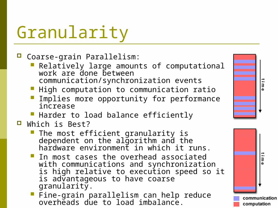
Granularity Coarse-grain Parallelism:

Relatively large amounts of computational work are done between communication/synchronization events

High computation to communication ratio Implies more opportunity for performance

increase Harder to load balance efficiently

Which is Best? The most efficient granularity is dependent on

the algorithm and the hardware environment in which it runs.

In most cases the overhead associated with communications and synchronization is high relative to execution speed so it is advantageous to have coarse granularity.

Fine-grain parallelism can help reduce overheads due to load imbalance.

67

I/O The Bad News:

I/O operations are generally regarded as inhibitors to parallelism

Parallel I/O systems are immature or not available for all platforms

In an environment where all tasks see the same filespace, write operations will result in file overwriting

Read operations will be affected by the fileserver's ability to handle multiple read requests at the same time

I/O that must be conducted over the network (NFS, non-local) can cause severe bottlenecks

The Good News: Some parallel file systems are available. For example: GPFS, L

ustre, PVFS, PanFS, HP SFS, GFS ..etc The parallel I/O programming interface specification for MPI

has been available since 1996 as part of MPI-2. Vendor and "free" implementations are now commonly available.

68

Speedup Factor How much faster the multiprocessor solves the problem?

We defined the speedup factor S(p) which is a measure of relative performance

Maximum speedup (linear speedup)

Superlinear speedup S(p) > p

p

s

t

t

ppS

processors ssor with multiproce a using timeExecution

systemprocessor single using timeExecution )(

ppt

tpS

s

s /

)(

69

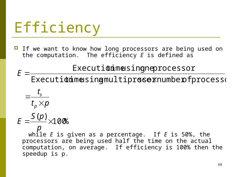
Efficiency If we want to know how long processors are being used on

the computation. The efficiency E is defined as

while E is given as a percentage. If E is 50%, the processors are being used half the time on the actual computation, on average. If efficiency is 100% then the speedup is p.

%100)(

processors ofnumber ssor multiproce a using timeExecution

processor one using timeExecution

p

pSE

pt

t

E

p

s

70

Overheads Several factors will appear as overhead in the parallel computation

Periods when not all the processors can be performing useful work

Extra computations in the parallel version Communication time between processors

Assume the fraction of the computation that cannot be divided in to concurrent tasks is f.

The time used to perform computation with p processors is

ptfftt ssp /)1( fts (1-f)ts1 CPU

(1-f)ts/p

p CPUs

serial section

serial section

Parallelizable sections

71

Amdahl’s Law The speedup factor is given as

fpS

fp

p

ptfft

tpS

p

ss

s

1)(

)1(1/)1()(

72

Complexity In general, parallel applications are much more complex than co

rresponding serial applications, perhaps an order of magnitude. Not only do you have multiple instruction streams executing at the same time, but you also have data flowing between them.

The costs of complexity are measured in programmer time in virtually every aspect of the software development cycle: Design Coding Debugging Tuning Maintenance

Adhering to "good" software development practices is essential when when working with parallel applications - especially if somebody besides you will have to work with the software.

73

Portability Thanks to standardization in several APIs, such as MPI, POSIX thr

eads, HPF and OpenMP, portability issues with parallel programs are not as serious as in years past. However...

All of the usual portability issues associated with serial programs apply to parallel programs. For example, if you use vendor "enhancements" to Fortran, C or C++, portability will be a problem.

Even though standards exist for several APIs, implementations will differ in a number of details, sometimes to the point of requiring code modifications in order to effect portability.

Operating systems can play a key role in code portability issues. Hardware architectures are characteristically highly variable and

can affect portability.

74

Resource Requirements The primary intent of parallel programming is to decrease

execution wall clock time, however in order to accomplish this, more CPU time is required. For example, a parallel code that runs in 1 hour on 8 processors actually uses 8 hours of CPU time.

The amount of memory required can be greater for parallel codes than serial codes, due to the need to replicate data and for overheads associated with parallel support libraries and subsystems.

For short running parallel programs, there can actually be a decrease in performance compared to a similar serial implementation. The overhead costs associated with setting up the parallel environment, task creation, communications and task termination can comprise a significant portion of the total execution time for short runs.

75

Scalibility The ability of a parallel program's performance to scale is a resul

t of a number of interrelated factors. Simply adding more machines is rarely the answer.

The algorithm may have inherent limits to scalability. At some point, adding more resources causes performance to decrease. Most parallel solutions demonstrate this characteristic at some point.

Hardware factors play a significant role in scalability. Examples: Memory-cpu bus bandwidth on an SMP machine Communications network bandwidth Amount of memory available on any given machine or set of machin

es Processor clock speed

Parallel support libraries and subsystems software can limit scalability independent of your application.

76

Example his example demonstrates calculations on 2-dimensio

nal array elements, with the computation on each array element being independent from other array elements.

The serial program calculates one element at a time in sequential order.

Serial code could be of the form: do j = 1,n do i = 1,n

a(i,j) = fcn(i,j) end do end do The calculation of elements is independent of one ano

ther - leads to an embarrassingly parallel situation. The problem should be computationally intensive.

77

Array Processing Parallel Solution 1

Arrays elements are distributed so that each processor owns a portion of an array (subarray).

Independent calculation of array elements insures there is no need for communication between tasks.

Distribution scheme is chosen by other criteria, e.g. unit stride (stride of 1) through the subarrays. Unit stride maximizes cache/memory usage.

Since it is desirable to have unit stride through the subarrays, the choice of a distribution scheme depends on the programming language. See the Block - Cyclic Distributions Diagram for the options.

After the array is distributed, each task executes the portion of the loop corresponding to the data it owns. For example, with Fortran block distribution:

do j = mystart, myend do i = 1,n a(i,j) = fcn(i,j) end do end do

Notice that only the outer loop variables are different from the serial solution.

78

Solution Implement as SPMD

model. Master process

initializes array, sends info to worker processes and receives results.

Worker process receives info, performs its share of computation and sends results to master.

Using the Fortran storage scheme, perform block distribution of the array.

find out if I am MASTER or WORKER if I am MASTER initialize the array send each WORKER info on part of array it owns send each WORKER its portion of initial array receive from each WORKER results else if I am WORKER receive from MASTER info on part of array I own receive from MASTER my portion of initial array # calculate my portion of array do j = my first column,my last column do i = 1,n a(i,j) = fcn(i,j) end do end do send MASTER results endif

79

Array Processing Parallel Solution 2: Pool of Tasks The previous array solution demonstrated static load balancing: Each task has a fixed amount of work to do May be significant idle time for faster or more lightly loaded

processors - slowest tasks determines overall performance. Static load balancing is not usually a major concern if all tasks are

performing the same amount of work on identical machines. If you have a load balance problem (some tasks work faster than

others), you may benefit by using a "pool of tasks" scheme. Pool of Tasks Scheme: Two processes are employed Master Process:

Holds pool of tasks for worker processes to do Sends worker a task when requested Collects results from workers

Worker Process: repeatedly does the following Gets task from master process Performs computation Sends results to master

80

Pool of Tasks Scheme: Worker processes

do not know before runtime which portion of array they will handle or how many tasks they will perform.

Dynamic load balancing occurs at run time: the faster tasks will get more work to do.

find out if I am MASTER or WORKER

if I am MASTER do until no more jobs send to WORKER next job receive results from WORKER end do tell WORKER no more jobs else if I am WORKER do until no more jobs receive from MASTER next job calculate array element: a(i,j) = fcn(i,j) send results to MASTER end do endif

81

PI Calculationnpoints = 10000 circle_count = 0

do j = 1,npoints generate 2 random numbers between 0 and

1 xcoordinate = random1 ycoordinate = random2 if (xcoordinate, ycoordinate) inside circle then circle_count = circle_count + 1 end do

PI = 4.0*circle_count/npoints

82

PI CalculationParallel Solution

npoints = 10000 circle_count = 0 p = number of tasks num = npoints/p find out if I am MASTER or WORKER do j = 1,num

generate 2 random numbers between 0 and 1 xcoordinate = random1 ycoordinate = random2 if (xcoordinate, ycoordinate) inside circle then circle_count = circle_count + 1 end do if I am MASTER receive from WORKERS their circle_counts compute PI (use MASTER and WORKER calculations) else if I am WORKER send to MASTER circle_count endif

83

Simple Heat Equation

do iy = 2, ny - 1

do ix = 2, nx - 1

u2(ix, iy) = u1(ix, iy) +

cx * (u1(ix+1,iy) + u1(ix-1,iy)- 2.*u1(ix,iy)) +

cy * (u1(ix,iy+1) + u1(ix,iy-1) - 2.*u1(ix,iy))

end do

end do

84

Simple Heat EquationParallel Solution 1

Determine data dependencies interior elements belonging to a task are independent of other tasks border elements are dependent upon a neighbor task's data, necessitating communication.

find out if I am MASTER or WORKER if I am MASTER initialize array send each WORKER starting info and subarray do until all WORKERS converge gather from all WORKERS convergence data broadcast to all WORKERS convergence signal end do receive results from each WORKER else if I am WORKER receive from MASTER starting info and subarray do until solution converged update time send neighbors my border info receive from neighbors their border info update my portion of solution array determine if my solution has converged send MASTER convergence data receive from MASTER convergence signal end do send MASTER results endif

85

Simple Heat EquationParallel Solution 2: Overlapping Communication and Computationfind out if I am MASTER or WORKER if I am MASTER initialize array send each WORKER starting info and subarray do until all WORKERS converge gather from all WORKERS convergence data broadcast to all WORKERS convergence signal end do receive results from each WORKER else if I am WORKER receive from MASTER starting info and subarray do until solution converged update time non-blocking send neighbors my border info non-blocking receive neighbors border info update interior of my portion of solution array wait for non-blocking communication complete update border of my portion of solution array determine if my solution has converged send MASTER convergence data receive from MASTER convergence signal end do send MASTER results endif

86

1-D Wave Equation In this example, the amplitude along a uniform, vibrating string is calculated

after a specified amount of time has elapsed. The calculation involves:

the amplitude on the y axis i as the position index along the x axis node points imposed along the string update of the amplitude at discrete time steps.

The equation to be solved is the one-dimensional wave equation: A(i,t+1) = (2.0 * A(i,t)) - A(i,t-1) + (c * (A(i-1,t) - (2.0 * A(i,t)) + A(i+1,t))) where c is a constant

Note that amplitude will depend on previous timesteps (t, t-1) and neighboring points (i-1, i+1). Data dependence will mean that a parallel solution will involve communications.

87

1-D Wave EquationParallel Solution

find out number of tasks and task identities

#Identify left and right neighbors left_neighbor = mytaskid - 1 right_neighbor = mytaskid +1 if mytaskid = first thenleft_neigbor = last if mytaskid = last thenright_neighbor = first find out if I am MASTER or WORKER if I am MASTER initialize array send each WORKER starting info and s

ubarray else if I am WORKER receive starting info and subarray fr

om MASTERendif

#Update values for each point along string #In this example the master participates in

calculations do t = 1, nsteps send left endpoint to left neighbor receive left endpoint from right neighbor send right endpoint to right neighbor receive right endpoint from left neighbor #Update points along line do i = 1, npoints newval(i) = (2.0 * values(i)) - oldval

(i) + (sqtau * (values(i-1) - (2.0 * values(i)) + values(i+1)))

end do end do #Collect results and write to file if I am MASTER receive results from each WORKER write results to file else if I am WORKER send results to MASTER endif

88

References

“Parallel Programming” by Barry Wilkinson and Michael Allen

“Introduction to Parallel Computing” by Ananth Grama, Anshul Gupta, George Karypis, and Vipin Kumar

Web site from LLNL tutorials(http://www.llnl.gov/computing/hpc/training/)