Introduction to Optimization

Second Edition

Alan ParksDepartment of MathematicsLawrence University

♠ This project puts text material, carefully coordinated with lecturesand homework, into the hands of upper level students at cost. It wasbegun in September 1997 and has been revised and expanded manytimes since.

c©Alan Parks. All rights reserved. No portion of this work may bereproduced, stored in a retrieval system, or transmitted in any form,or by any means, electronic, mechanical, photocopying, recording, orotherwise, without the prior consent of the author. The principal copyof this work was printed on July 22, 2014.

Contents

Introduction. iii

Chapter 1. Linear Algebra 11. Matrix Operations 12. Reduced Form and Replacement 53. Linear Equations 104. Inverses 135. Technical Lemmas 16

Chapter 2. Linear Optimization 211. Definitions and Basic Solutions 212. Canonical Simplex 283. Feasibility 354. The Linear Algebra of Primal Form 415. Duality 436. Perturbation and Shadow Prices 497. Applications 54

Chapter 3. Multivariate Calculus 671. Open Sets and Continuous Functions 672. Limit Points and Extreme Values 743. Derivatives 774. Implicit Curves 87

Chapter 4. Non-linear Optimization 951. Introduction 952. Full Row Rank 993. The Kuhn-Tucker Conditions 1004. Applications 108

i

ii CONTENTS

Chapter 5. Convex Sets and Functions 1131. Introduction 1132. The Hessian 119

Chapter 6. Convex Optimization 1251. The Sufficiency of Kuhn-Tucker 1252. Applications 1283. Local Minima 131

Bibliography 135

Index 137

Introduction.

Optimization problems, traditionally called mathematical programs seekthe maximum or minimum value of a function over a domain defined by equa-tions and inequalities. It has become standard to call this function the ob-jective.1 Over the first part of the course we will study linear optimizationproblems – a class that includes a great many applications. To whet yourappetite, we mention that zero-sum linear games are linear optimization prob-lems, as are many problems of resource allocation, production mixture, projectscheduling, and transportation networks. There is a definitive algorithm forsolving linear programs; we will work toward a thorough understanding ofthis algorithm, emphasizing how particular aspects of a solution inform ourunderstanding of the original problem beyond just having the solution in hand.

Our work on linear problems will involve a version of the Kuhn-Tuckerconditions that are key to understanding non-linear problems. The linearversion of Kuhn-Tucker will lead to the notion of duality – that a given linearproblem is actually two problems in one. Furthermore, we will see how topredict what happens to the solution of a problem when small changes aremade in the problem parameters.

Another main section of the course will involve non-linear optimizationproblems, where the emphasis is less on obtaining explicit solutions as ondeveloping the Kuhn-Tucker conditions and the technical hypothesis underwhich they hold. These conditions clarify and generalize both the role ofcritical points and the use of the Lagrange multiplier equations in calculus.We will again address the effect of changes in problem parameters.

We will next turn to the convex problems, a class that lives in a sense be-tween the linear and general non-linear problems. In many applied optimiza-tion problems, there are theoretical reasons for assuming convexity. When

1Notice that the objective of an optimization problem is a quantity, not a desired out-come. This possibly confusing useage has become standard.

iii

iv INTRODUCTION.

the Kuhn-Tucker conditions hold in a convex problem, we necessarily have asolution; this reduces the problem to the problem of solving equations.

The theory of linear optimization is supported by linear algebra, the non-linear optimization by the multivariate calculus, and the convex programmingby the theory of convex sets and functions. Attaining the needed technicalunderpinnings in these subjects will necessitate some serious review as well asthe introduction of advanced techniques, including a version of what is calledthe Implicit Curve Theorem. We will address this material in three substantialchapters of the text.

As usual, you will need to study the text actively. There are problemsinterspersed throughout the text; some will be assigned as homework – youshould do as many of them as you can in any case. Because the amount ofreview (especially of the linear algebra) will vary from student to student,make sure you have a thorough understanding of the reasoning given in theproofs of the main theorems.

We will use a programmed solver to do much of the computational work,always remembering how much is gained by slogging through both represen-tative and abstract problems by hand!

CHAPTER 1

Linear Algebra

We lay out the matrix facts we need for optimization. We will begin

with the matrix arithmetic covered rather briskly, and then we will veer into

fun technicalities. The book [3]1 contains a more elementary version of this

material.

1. Matrix Operations

For positive integers m,n, an m × n matrix is a table of numbers with

m rows and n columns. We say that m × n is the size of the matrix. For a

matrix A, its i, j-entry is denoted A[i, j], for 1 ≤ i ≤ m and 1 ≤ j ≤ n. We

find the bracket notation A[i, j] to be more readable than the commonly used

subscript notation: Ai,j.

Two matrices are equal if they have the same size and if corresponding

entries are equal (as numbers). This may seem trivial, or perhaps obvious,

but it carries some important subtleties.

Because of the frequent appearance of inequalities in our work, we will find

it useful to write A ≤ B for m×n matrices A,B when we have A[i, j] ≤ B[i, j]

for all possible i, j. Similarly, A ≥ B means that each entry in A is greater

than or equal to the corresponding entry in B. Notice that A 6≤ B does not

imply A ≥ B. (Example?)

It is common in applied work to identify Rn with the set of n× 1 matrices

– or with the set of 1 × n matrices. We will usually prefer to write elements

of Rn as columns, but we will be clear in each case.

1Boldface letters in brackets refer to entries in the bibliography on p.135.

1

2 1. LINEAR ALGEBRA

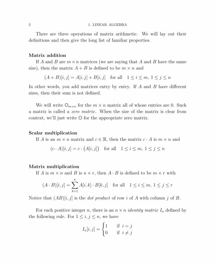
There are three operations of matrix arithmetic. We will lay out their

definitions and then give the long list of familiar properties.

Matrix addition

If A and B are m×n matrices (we are saying that A and B have the same

size), then the matrix A+B is defined to be m× n and

(A+B)[i, j] = A[i, j] +B[i, j] for all 1 ≤ i ≤ m, 1 ≤ j ≤ n

In other words, you add matrices entry by entry. If A and B have different

sizes, then their sum is not defined.

We will write Om×n for the m× n matrix all of whose entries are 0. Such

a matrix is called a zero matrix . When the size of the matrix is clear from

context, we’ll just write O for the appropriate zero matrix.

Scalar multiplication

If A is an m× n matrix and c ∈ R, then the matrix c · A is m× n and

(c · A)[i, j] = c ·(A[i, j]

)for all 1 ≤ i ≤ m, 1 ≤ j ≤ n

Matrix multiplication

If A is m× n and B is n× r, then A ·B is defined to be m× r with

(A ·B)[i, j] =n∑

k=1

A[i, k] ·B[k, j] for all 1 ≤ i ≤ m, 1 ≤ j ≤ r

Notice that (AB)[i, j] is the dot product of row i of A with column j of B.

For each positive integer n, there is an n×n identity matrix In defined by

the following rule. For 1 ≤ i, j ≤ n, we have

In[i, j] =

{1 if i = j

0 if i 6= j

1. MATRIX OPERATIONS 3

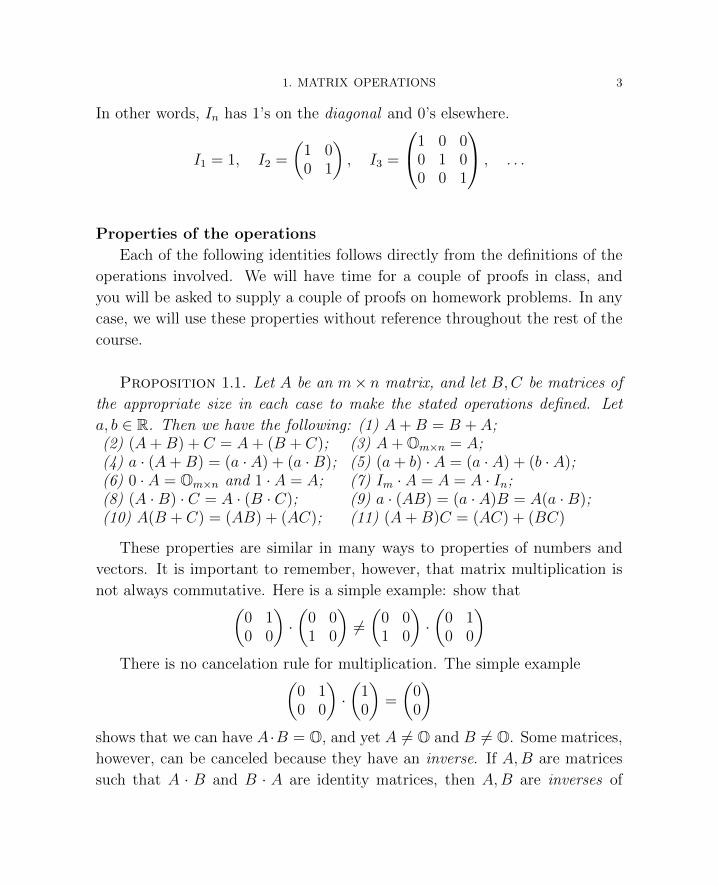
In other words, In has 1’s on the diagonal and 0’s elsewhere.

I1 = 1, I2 =

(1 00 1

), I3 =

1 0 00 1 00 0 1

, . . .

Properties of the operations

Each of the following identities follows directly from the definitions of the

operations involved. We will have time for a couple of proofs in class, and

you will be asked to supply a couple of proofs on homework problems. In any

case, we will use these properties without reference throughout the rest of the

course.

Proposition 1.1. Let A be an m× n matrix, and let B,C be matrices of

the appropriate size in each case to make the stated operations defined. Let

a, b ∈ R. Then we have the following: (1) A+B = B + A;(2) (A+B) + C = A+ (B + C); (3) A+ Om×n = A;(4) a · (A+B) = (a · A) + (a ·B); (5) (a+ b) · A = (a · A) + (b · A);(6) 0 · A = Om×n and 1 · A = A; (7) Im · A = A = A · In;(8) (A ·B) · C = A · (B · C); (9) a · (AB) = (a · A)B = A(a ·B);(10) A(B + C) = (AB) + (AC); (11) (A+B)C = (AC) + (BC)

These properties are similar in many ways to properties of numbers and

vectors. It is important to remember, however, that matrix multiplication is

not always commutative. Here is a simple example: show that(0 10 0

)·(

0 01 0

)6=(

0 01 0

)·(

0 10 0

)There is no cancelation rule for multiplication. The simple example(

0 10 0

)·(

10

)=

(00

)shows that we can have A ·B = O, and yet A 6= O and B 6= O. Some matrices,

however, can be canceled because they have an inverse. If A,B are matrices

such that A · B and B · A are identity matrices, then A,B are inverses of

4 1. LINEAR ALGEBRA

each other. A matrix that has an inverse is called an invertible matrix. In the

equation A · C = D, if A has an inverse B, then

B · A · C = B ·D so that C = B ·D

Later, we will show that an invertible matrix has to be square – it has the

same number of rows as columns. For now, we will prove that inverses are

unique. For if B,C are both inverses of A, then using I for the identity

matrix of appropriate size and using Proposition 1.1(8) (the associative law of

multiplication), we see that

B = B · I = B · (A · C) = (B · A) · C = I · C = C

It will not surprise you that we write the unique inverse of A as A−1.

♦ Problem 1

Suppose that the matrix J satisfies J ·A = A for all m× n matrices A. Show

that J = Im.

♦

♦ Problem 2

Show that if A and B invert, then so does A ·B. (Hint: use the inverses of A

and B to get the inverse of A ·B, but remember that multiplication is

usually not commutative.)

♦

♦ Problem 3

Show, by finding explicit examples, that there are infinitely many matrices A

such that A2 = I2.

♦

♦ Problem 4

Suppose that A and B are m× n, and that AX = BX for all n× 1 matrices

X. Then A = B.

♦

2. REDUCED FORM AND REPLACEMENT 5

Transpose

We will need one more operation: the transpose. Given the m× n matrix

A, its transpose AT is the n ×m matrix with AT [i, j] = A[j, i] for 1 ≤ i ≤ n

and 1 ≤ j ≤ m. Thus, AT writes each row of A as a column, and each column

of A as a row.

Here are the properties of the transpose; as with Proposition 1.1, the proofs

will be left partly to class and partly to homework.

Proposition 1.2. Let A,B be matrices of the appropriate size in each case

to make the stated operations defined. Let a ∈ R. Then we have the following.

(a) (AT )T = A

(b) (A+B)T = (AT ) + (BT )

(c) (a · A)T = a · (AT )

(d) (A ·B)T = (BT ) · (AT )

♦ Problem 5

Let A be an n× n matrix, and define f : Rn → R by f(X) = XT · A ·X(writing X as a column).

(a) Show that if AT is used in place of A in the definition of f , then the

same function results.

(b) Let B = (A+AT )/2. Show that BT = B and that if B is used in place of

A in the definition of f , then the same function results.

♦

2. Reduced Form and Replacement

Matrices will arise in this course in the context of linear equations. If A

is m × n and B is m × 1, the equation A · X = B, where X is an unknown

n × 1 matrix, is a linear equation with coefficient matrix A and right side

B. The reader probably knows how to use elimination, often called Gaussian

elimination or Gauss-Jordan elimination to solve linear equations. We will

6 1. LINEAR ALGEBRA

describe this technique as a way of transforming a matrix into a specific form

called reduced form. The matrix A is in reduced form if it has two properties:

(1) Any zero rows of A are grouped at the bottom.

(2) For each non-zero row j of A, there is a basic column cj such that

A[j, cj] = 1 and where A[k, cj] = 0 for all k 6= j.

Every identity matrix is in reduced form. So are all the zero matrices. Here

are some other examples.0 3 11 −4 00 0 0

,

(1 1 1 02 0 3 1

),

(3 4 1 10 0 0 0

)The example on the far right shows that c1 could be either 3 or 4. In other

words, the columns cj are not uniquely determined by the reduced form. When

we speak of reduced form, however, we assume that particular choices of those

columns have been made.2 The rank of a matrix in reduced form is the number

of non-zero rows it has. (Every zero matrix has rank 0.)

The main theoretical fact: for each matrix A, there is an invertible matrix

R such that R · A is in reduced form. To prove this and to show how to find

such a matrix R, we introduce the elementary operations that are done on the

rows of a given matrix:

Elementary operations

(1) Multiplying a row by a non-zero number.

(2) Adding a multiple of one row to another (leaving the first row un-

changed).

(3) Switching two rows.

The elementary operations are actually multiplication on the left by an

invertible matrix.

2So, technically speaking, we are in reduced form if there is a list of distinct basiccolumns for which the stated properties hold.

2. REDUCED FORM AND REPLACEMENT 7

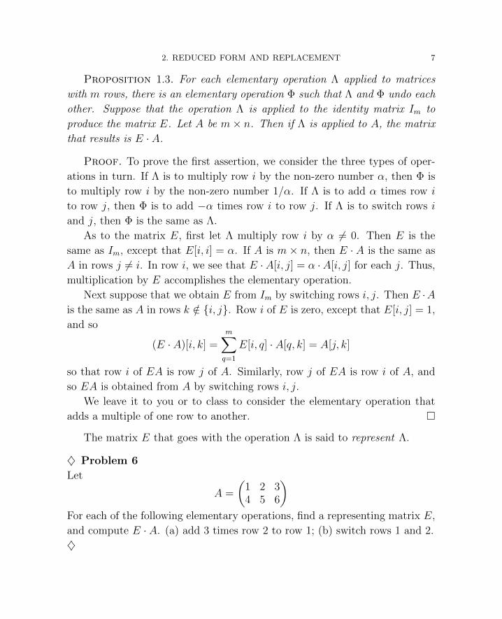
Proposition 1.3. For each elementary operation Λ applied to matrices

with m rows, there is an elementary operation Φ such that Λ and Φ undo each

other. Suppose that the operation Λ is applied to the identity matrix Im to

produce the matrix E. Let A be m× n. Then if Λ is applied to A, the matrix

that results is E · A.

Proof. To prove the first assertion, we consider the three types of oper-

ations in turn. If Λ is to multiply row i by the non-zero number α, then Φ is

to multiply row i by the non-zero number 1/α. If Λ is to add α times row i

to row j, then Φ is to add −α times row i to row j. If Λ is to switch rows i

and j, then Φ is the same as Λ.

As to the matrix E, first let Λ multiply row i by α 6= 0. Then E is the

same as Im, except that E[i, i] = α. If A is m × n, then E · A is the same as

A in rows j 6= i. In row i, we see that E ·A[i, j] = α ·A[i, j] for each j. Thus,

multiplication by E accomplishes the elementary operation.

Next suppose that we obtain E from Im by switching rows i, j. Then E ·Ais the same as A in rows k /∈ {i, j}. Row i of E is zero, except that E[i, j] = 1,

and so

(E · A)[i, k] =m∑q=1

E[i, q] · A[q, k] = A[j, k]

so that row i of EA is row j of A. Similarly, row j of EA is row i of A, and

so EA is obtained from A by switching rows i, j.

We leave it to you or to class to consider the elementary operation that

adds a multiple of one row to another. �

The matrix E that goes with the operation Λ is said to represent Λ.

♦ Problem 6

Let

A =

(1 2 34 5 6

)For each of the following elementary operations, find a representing matrix E,

and compute E · A. (a) add 3 times row 2 to row 1; (b) switch rows 1 and 2.

♦

8 1. LINEAR ALGEBRA

Suppose that an elementary operation Λ is applied to Im to produce the

matrix E. Applying the inverse operation Φ to E we get Im. On the other

hand, the inverse operation is accomplished by multiplying by a matrix F .

Thus F ·E = Im. Moreover, if we do Φ and then Λ, we also get Im back again.

Thus, E · F = Im. In other words, E,F are inverses.

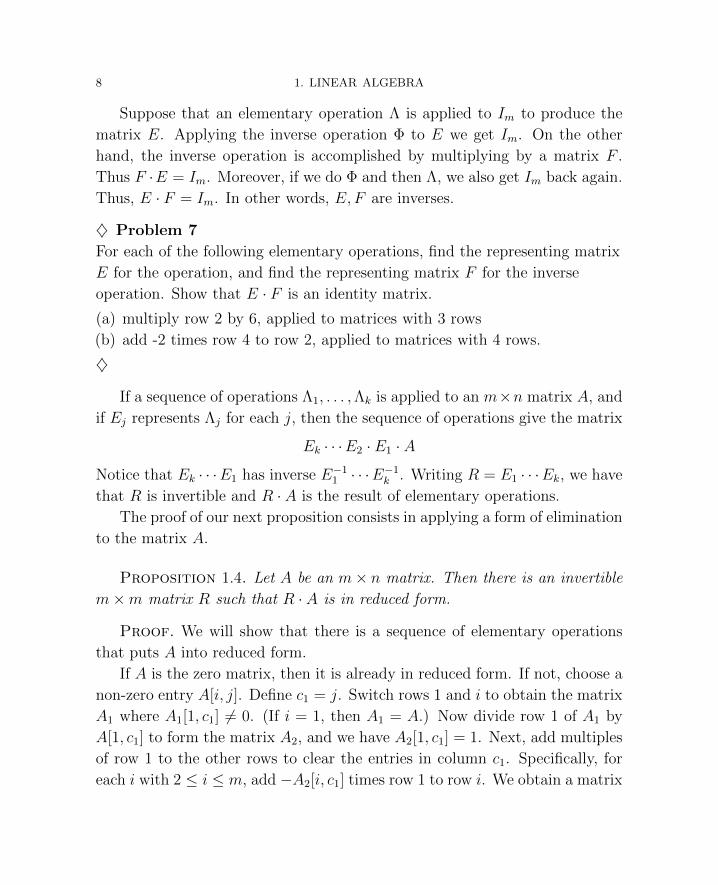
♦ Problem 7

For each of the following elementary operations, find the representing matrix

E for the operation, and find the representing matrix F for the inverse

operation. Show that E · F is an identity matrix.

(a) multiply row 2 by 6, applied to matrices with 3 rows

(b) add -2 times row 4 to row 2, applied to matrices with 4 rows.

♦

If a sequence of operations Λ1, . . . ,Λk is applied to an m×n matrix A, and

if Ej represents Λj for each j, then the sequence of operations give the matrix

Ek · · ·E2 · E1 · A

Notice that Ek · · ·E1 has inverse E−11 · · ·E−1k . Writing R = E1 · · ·Ek, we have

that R is invertible and R · A is the result of elementary operations.

The proof of our next proposition consists in applying a form of elimination

to the matrix A.

Proposition 1.4. Let A be an m× n matrix. Then there is an invertible

m×m matrix R such that R · A is in reduced form.

Proof. We will show that there is a sequence of elementary operations

that puts A into reduced form.

If A is the zero matrix, then it is already in reduced form. If not, choose a

non-zero entry A[i, j]. Define c1 = j. Switch rows 1 and i to obtain the matrix

A1 where A1[1, c1] 6= 0. (If i = 1, then A1 = A.) Now divide row 1 of A1 by

A[1, c1] to form the matrix A2, and we have A2[1, c1] = 1. Next, add multiples

of row 1 to the other rows to clear the entries in column c1. Specifically, for

each i with 2 ≤ i ≤ m, add −A2[i, c1] times row 1 to row i. We obtain a matrix

2. REDUCED FORM AND REPLACEMENT 9

A3 where A3[1, c1] = 1 and A3[i, c1] = 0 for i ≥ 2. And A3 was obtained from

A by a sequence of elementary operations.

We continue, looking for a non-zero entry in row 2 or below. If there

are non-zero entries here, we choose one A3[i, c2]. Notice that c2 6= c1, since

A[i, c1] = 0. Switch rows if necessary to bring this entry to row 2, divide row 2

by the entry, and add multiples of row 2 to other rows to clear out column c2.

These operations will not affect column c1, since that column is zero except

for A[1, c1] = 1.

This procedure can be applied below row 2, and then below row 3, and so

on, until either we hit the bottom row or we end up with rows of 0’s. The

resulting matrix is in reduced form, and it was obtained from A by a sequence

of elementary operations. The discussion right before this proof finds the

required invertible matrix. �

An invertible matrix R such that R·A is in reduced form is called a reducing

matrix for A. The matrix R · A is a reduced form for the matrix A. We will

usually need merely the existence of a reducing matrix – we will rarely need

to find it explicitly. Nonetheless, it is a good exercise to compute a couple of

them to make sure you can put together the relevant facts. Proposition 1.4

shows how to perform elementary operations on an m × n matrix A to put

it into reduced form, row by row. Suppose we perform the same operations

in the same order starting with the identity matrix Im, so that the matrix R

results. Proposition 1.3 shows that the matrix R that results from Im is a

reducing matrix for A.

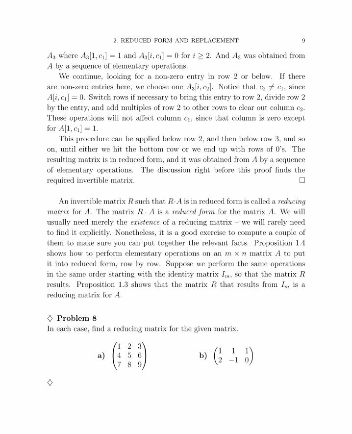
♦ Problem 8

In each case, find a reducing matrix for the given matrix.

a)

1 2 34 5 67 8 9

b)

(1 1 12 −1 0

)

♦

10 1. LINEAR ALGEBRA

Proposition 1.4 finds a particular reduced form for a given matrix. A

matrix will have, in general, many reduced forms. We need to see how to

change one form into another using replacement.

Suppose that the m × n matrix A is in reduced form, and let A[j, cj] = 1

for 1 ≤ j ≤ k, where the rows of A below row k are all 0. Suppose that j ≤ k

and A[j, p] 6= 0 for some p 6= cj. We can perform elementary row operations

to get a new reduced form in which A[j, p] replaces A[j, cj]. Here’s what we

do:

(1) Divide row j by A[j, p] to form the matrix A1 with A1[j, p] = 1.

(2) Add multiples of row j to the other rows to form the matrix A2 with

A2[i, p] = 0 for all i 6= j. (Specifically, add −A1[i, p] times row j to

row i, for each i 6= j.)

Notice that in the matrix A2 that results, we have A2[q, cq] = 1 for all q 6= j,

and column cq of A2 is still 0 except for the entry at row q. This is because

the row operations just described do not affect column cq. We describe the

process of going from A to A2 as replacement and we say we replace column

cj by column p.

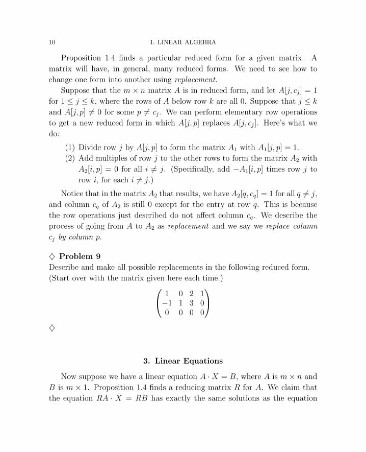
♦ Problem 9

Describe and make all possible replacements in the following reduced form.

(Start over with the matrix given here each time.) 1 0 2 1−1 1 3 00 0 0 0

♦

3. Linear Equations

Now suppose we have a linear equation A ·X = B, where A is m× n and

B is m × 1. Proposition 1.4 finds a reducing matrix R for A. We claim that

the equation RA · X = RB has exactly the same solutions as the equation

3. LINEAR EQUATIONS 11

AX = B. Indeed, if AX = B, then certainly RAX = RB. Conversely, if

RAX = RB, then since R is invertible, we have

AX = R−1RAX = R−1RB = B

As an alternative to finding a reducing matrix, we can simply perform elemen-

tary operations on both A,B to bring the A-part into reduced form. As we

mentioned above, such a process constitutes elimination in its various forms.

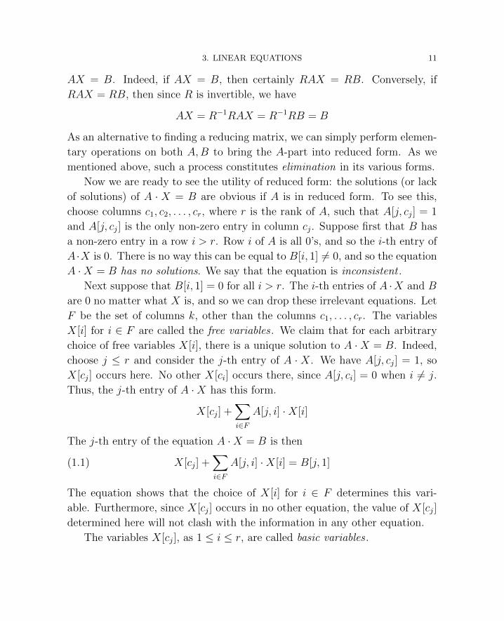
Now we are ready to see the utility of reduced form: the solutions (or lack

of solutions) of A · X = B are obvious if A is in reduced form. To see this,

choose columns c1, c2, . . . , cr, where r is the rank of A, such that A[j, cj] = 1

and A[j, cj] is the only non-zero entry in column cj. Suppose first that B has

a non-zero entry in a row i > r. Row i of A is all 0’s, and so the i-th entry of

A ·X is 0. There is no way this can be equal to B[i, 1] 6= 0, and so the equation

A ·X = B has no solutions. We say that the equation is inconsistent .

Next suppose that B[i, 1] = 0 for all i > r. The i-th entries of A ·X and B

are 0 no matter what X is, and so we can drop these irrelevant equations. Let

F be the set of columns k, other than the columns c1, . . . , cr. The variables

X[i] for i ∈ F are called the free variables . We claim that for each arbitrary

choice of free variables X[i], there is a unique solution to A ·X = B. Indeed,

choose j ≤ r and consider the j-th entry of A · X. We have A[j, cj] = 1, so

X[cj] occurs here. No other X[ci] occurs there, since A[j, ci] = 0 when i 6= j.

Thus, the j-th entry of A ·X has this form.

X[cj] +∑i∈F

A[j, i] ·X[i]

The j-th entry of the equation A ·X = B is then

(1.1) X[cj] +∑i∈F

A[j, i] ·X[i] = B[j, 1]

The equation shows that the choice of X[i] for i ∈ F determines this vari-

able. Furthermore, since X[cj] occurs in no other equation, the value of X[cj]

determined here will not clash with the information in any other equation.

The variables X[cj], as 1 ≤ i ≤ r, are called basic variables .

12 1. LINEAR ALGEBRA

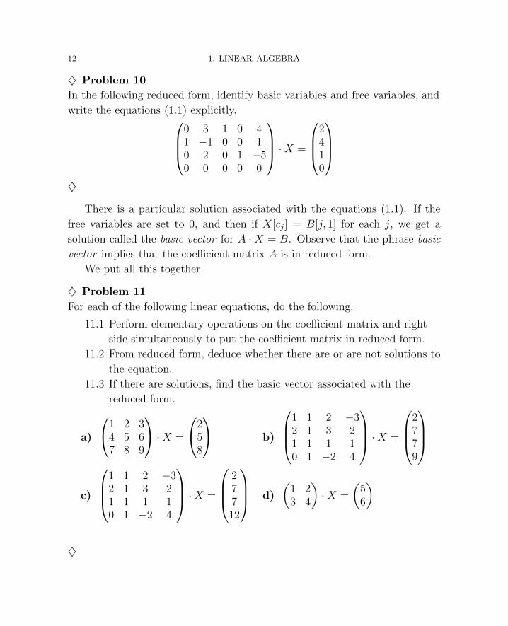
♦ Problem 10

In the following reduced form, identify basic variables and free variables, and

write the equations (1.1) explicitly.0 3 1 0 41 −1 0 0 10 2 0 1 −50 0 0 0 0

·X =

2410

♦

There is a particular solution associated with the equations (1.1). If the

free variables are set to 0, and then if X[cj] = B[j, 1] for each j, we get a

solution called the basic vector for A ·X = B. Observe that the phrase basic

vector implies that the coefficient matrix A is in reduced form.

We put all this together.

♦ Problem 11

For each of the following linear equations, do the following.

11.1 Perform elementary operations on the coefficient matrix and right

side simultaneously to put the coefficient matrix in reduced form.

11.2 From reduced form, deduce whether there are or are not solutions to

the equation.

11.3 If there are solutions, find the basic vector associated with the

reduced form.

a)

1 2 34 5 67 8 9

·X =

258

b)

1 1 2 −32 1 3 21 1 1 10 1 −2 4

·X =

2779

c)

1 1 2 −32 1 3 21 1 1 10 1 −2 4

·X =

27712

d)

(1 23 4

)·X =

(56

)

♦

4. INVERSES 13

Here is a summary of what we have done in this section. If we are given

an arbitrary linear equation A ·X = B, we can find a reducing matrix R for

A, and then the equation R · A · X = R · B has a reduced coefficient matrix

and the same solutions as the original equation. The reduced form allows us

to observe whether the equation has any solutions at all. If it does, then we

can write the basic variables in terms of the free variables to obtain the set of

solutions. It should be noted that if there are no free variables at all, then the

equation has a unique solution. We have also described replacement that gets

us from one reduced form to another; replacement will play a key role in the

solution of linear optimization problems, as we will see in Chapter 2.

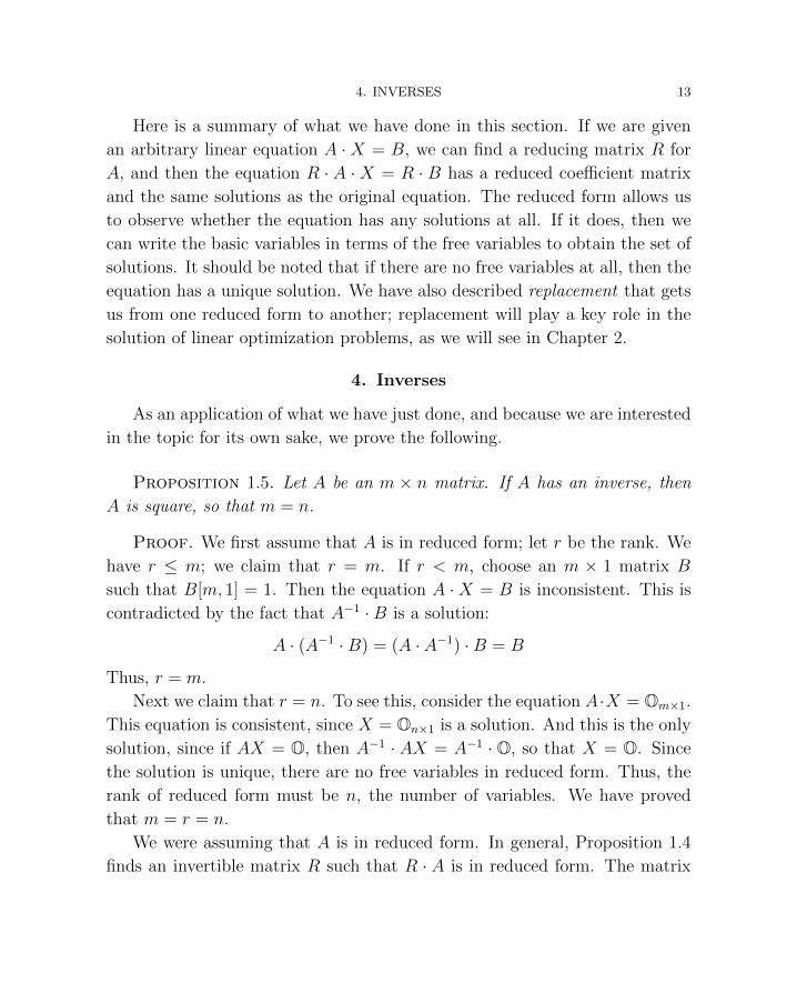
4. Inverses

As an application of what we have just done, and because we are interested

in the topic for its own sake, we prove the following.

Proposition 1.5. Let A be an m × n matrix. If A has an inverse, then

A is square, so that m = n.

Proof. We first assume that A is in reduced form; let r be the rank. We

have r ≤ m; we claim that r = m. If r < m, choose an m × 1 matrix B

such that B[m, 1] = 1. Then the equation A ·X = B is inconsistent. This is

contradicted by the fact that A−1 ·B is a solution:

A · (A−1 ·B) = (A · A−1) ·B = B

Thus, r = m.

Next we claim that r = n. To see this, consider the equation A·X = Om×1.

This equation is consistent, since X = On×1 is a solution. And this is the only

solution, since if AX = O, then A−1 · AX = A−1 · O, so that X = O. Since

the solution is unique, there are no free variables in reduced form. Thus, the

rank of reduced form must be n, the number of variables. We have proved

that m = r = n.

We were assuming that A is in reduced form. In general, Proposition 1.4

finds an invertible matrix R such that R · A is in reduced form. The matrix

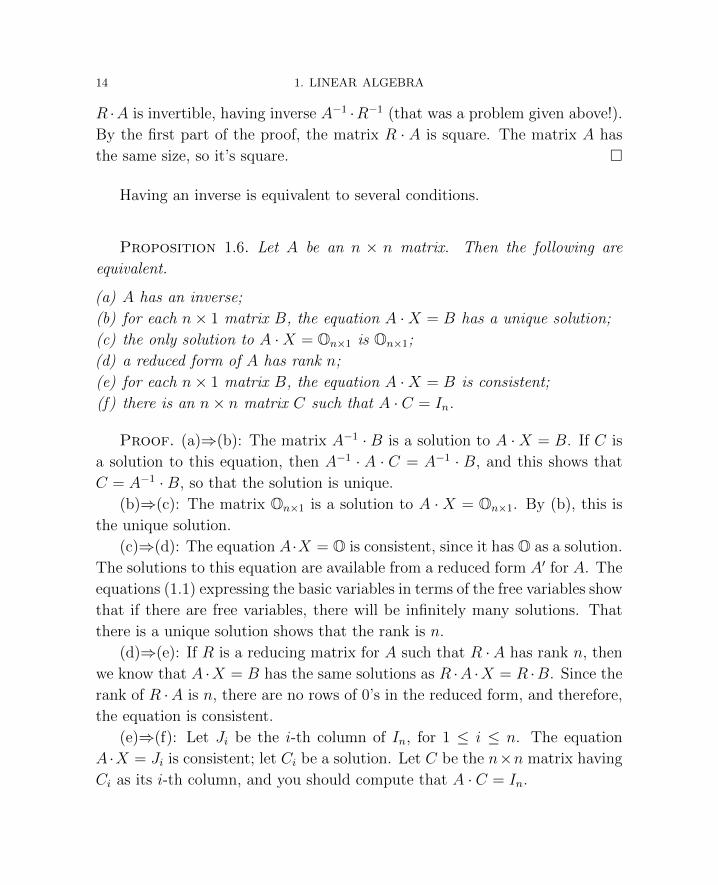
14 1. LINEAR ALGEBRA

R ·A is invertible, having inverse A−1 ·R−1 (that was a problem given above!).

By the first part of the proof, the matrix R · A is square. The matrix A has

the same size, so it’s square. �

Having an inverse is equivalent to several conditions.

Proposition 1.6. Let A be an n × n matrix. Then the following are

equivalent.

(a) A has an inverse;

(b) for each n× 1 matrix B, the equation A ·X = B has a unique solution;

(c) the only solution to A ·X = On×1 is On×1;

(d) a reduced form of A has rank n;

(e) for each n× 1 matrix B, the equation A ·X = B is consistent;

(f) there is an n× n matrix C such that A · C = In.

Proof. (a)⇒(b): The matrix A−1 · B is a solution to A ·X = B. If C is

a solution to this equation, then A−1 · A · C = A−1 · B, and this shows that

C = A−1 ·B, so that the solution is unique.

(b)⇒(c): The matrix On×1 is a solution to A ·X = On×1. By (b), this is

the unique solution.

(c)⇒(d): The equation A·X = O is consistent, since it has O as a solution.

The solutions to this equation are available from a reduced form A′ for A. The

equations (1.1) expressing the basic variables in terms of the free variables show

that if there are free variables, there will be infinitely many solutions. That

there is a unique solution shows that the rank is n.

(d)⇒(e): If R is a reducing matrix for A such that R ·A has rank n, then

we know that A ·X = B has the same solutions as R ·A ·X = R ·B. Since the

rank of R ·A is n, there are no rows of 0’s in the reduced form, and therefore,

the equation is consistent.

(e)⇒(f): Let Ji be the i-th column of In, for 1 ≤ i ≤ n. The equation

A ·X = Ji is consistent; let Ci be a solution. Let C be the n×n matrix having

Ci as its i-th column, and you should compute that A · C = In.

4. INVERSES 15

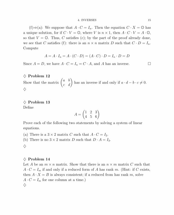
(f)⇒(a): We suppose that A · C = In. Then the equation C ·X = O has

a unique solution, for if C · V = O, where V is n× 1, then A · C · V = A ·O,

so that V = O. Thus, C satisfies (c); by the part of the proof already done,

we see that C satisfies (f): there is an n × n matrix D such that C ·D = In.

Compute

A = A · In = A · (C ·D) = (A · C) ·D = In ·D = D

Since A = D, we have A · C = In = C · A, and A has an inverse. �

♦ Problem 12

Show that the matrix

(a bc d

)has an inverse if and only if a · d− b · c 6= 0.

♦

♦ Problem 13

Define

A =

(1 2 34 5 6

)Prove each of the following two statements by solving a system of linear

equations.

(a) There is a 3× 2 matrix C such that A · C = I2.

(b) There is no 3× 2 matrix D such that D · A = I3.

♦

♦ Problem 14

Let A be an m× n matrix. Show that there is an n×m matrix C such that

A · C = Im if and only if a reduced form of A has rank m. (Hint: if C exists,

then A ·X = B is always consistent; if a reduced from has rank m, solve

A · C = Im for one column at a time.)

♦

16 1. LINEAR ALGEBRA

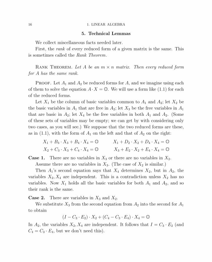
5. Technical Lemmas

We collect miscellaneous facts needed later.

First, the rank of every reduced form of a given matrix is the same. This

is sometimes called the Rank Theorem.

Rank Theorem. Let A be an m × n matrix. Then every reduced form

for A has the same rank.

Proof. Let A1 and A2 be reduced forms for A, and we imagine using each

of them to solve the equation A ·X = O. We will use a form like (1.1) for each

of the reduced forms.

Let X1 be the column of basic variables common to A1 and A2; let X2 be

the basic variables in A1 that are free in A2; let X3 be the free variables in A1

that are basic in A2; let X4 be the free variables in both A1 and A2. (Some

of these sets of variables may be empty; we can get by with considering only

two cases, as you will see.) We suppose that the two reduced forms are these,

as in (1.1), with the form of A1 on the left and that of A2 on the right:

X1 +B3 ·X3 +B4 ·X4 = O X1 +D2 ·X2 +D4 ·X4 = OX2 + C3 ·X3 + C4 ·X4 = O X3 + E2 ·X2 + E4 ·X4 = O

Case 1. There are no variables in X3 or there are no variables in X2.

Assume there are no variables in X3. (The case of X2 is similar.)

Then A1’s second equation says that X4 determines X2, but in A2, the

variables X2, X4 are independent. This is a contradiction unless X2 has no

variables. Now X1 holds all the basic variables for both A1 and A2, and so

their rank is the same.

Case 2. There are variables in X3 and X2.

We substitute X3 from the second equation from A2 into the second for A1

to obtain

(I − C3 · E2) ·X2 + (C4 − C3 · E4) ·X4 = OIn A2, the variables X2, X4 are independent. It follows that I = C3 · E2 (and

C4 = C3 · E4, but we don’t need this).

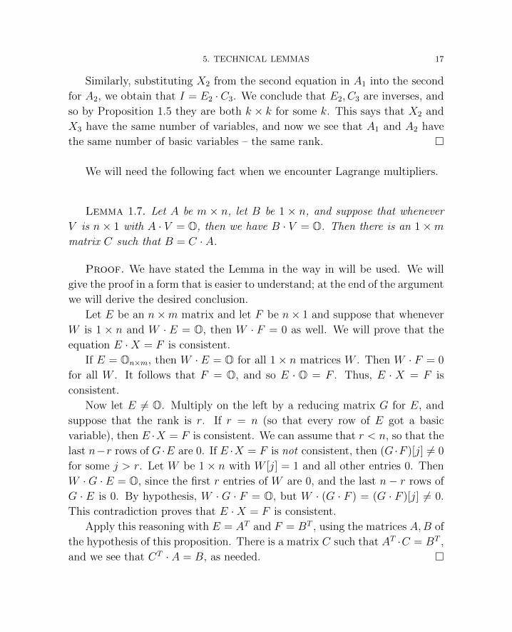
5. TECHNICAL LEMMAS 17

Similarly, substituting X2 from the second equation in A1 into the second

for A2, we obtain that I = E2 ·C3. We conclude that E2, C3 are inverses, and

so by Proposition 1.5 they are both k × k for some k. This says that X2 and

X3 have the same number of variables, and now we see that A1 and A2 have

the same number of basic variables – the same rank. �

We will need the following fact when we encounter Lagrange multipliers.

Lemma 1.7. Let A be m × n, let B be 1 × n, and suppose that whenever

V is n× 1 with A · V = O, then we have B · V = O. Then there is an 1×mmatrix C such that B = C · A.

Proof. We have stated the Lemma in the way in will be used. We will

give the proof in a form that is easier to understand; at the end of the argument

we will derive the desired conclusion.

Let E be an n×m matrix and let F be n× 1 and suppose that whenever

W is 1 × n and W · E = O, then W · F = 0 as well. We will prove that the

equation E ·X = F is consistent.

If E = On×m, then W · E = O for all 1× n matrices W . Then W · F = 0

for all W . It follows that F = O, and so E · O = F . Thus, E · X = F is

consistent.

Now let E 6= O. Multiply on the left by a reducing matrix G for E, and

suppose that the rank is r. If r = n (so that every row of E got a basic

variable), then E ·X = F is consistent. We can assume that r < n, so that the

last n−r rows of G ·E are 0. If E ·X = F is not consistent, then (G ·F )[j] 6= 0

for some j > r. Let W be 1× n with W [j] = 1 and all other entries 0. Then

W ·G · E = O, since the first r entries of W are 0, and the last n− r rows of

G · E is 0. By hypothesis, W · G · F = O, but W · (G · F ) = (G · F )[j] 6= 0.

This contradiction proves that E ·X = F is consistent.

Apply this reasoning with E = AT and F = BT , using the matrices A,B of

the hypothesis of this proposition. There is a matrix C such that AT ·C = BT ,

and we see that CT · A = B, as needed. �

18 1. LINEAR ALGEBRA

You are familiar with the dot product of vectors. If v, w ∈ Rn, then

v ◦ w =n∑

j=1

v[j] · w[j]

If we regard v, w as n × 1 matrices, then notice that v ◦ w = vT · w, where

the right hand product is matrix multiplication. You should know that the

dot product is symmetric, linear in both vectors, and that it commutes with

scalar multiplication.

We will also need the concept of norm of matrices in general and vectors

in particular. Given a vector v ∈ Rn, its norm is

|v| =

√√√√ n∑k=1

v[k]2

If we write v as an n× 1 matrix, we see that |v|2 = v ◦ v = vT · v.

An m × n matrix M has m · n entries, and so it can be considered as an

element of Rm·n. Then we have a natural norm:

|M | =

√√√√ m∑i=1

n∑j=1

M [i, j]2

When M is m×1 or 1×n, its matrix norm is obviously the same as its vector

norm.

We will need the following fact – the Cauchy-Schwarz Inequality .

Proposition 1.8. Let x, y ∈ Rn. Then

|x ◦ y| ≤ |x| · |y|

Proof. If |y| = 0, then y = O and both inequalities are trivial. We

assume that |y| 6= 0.

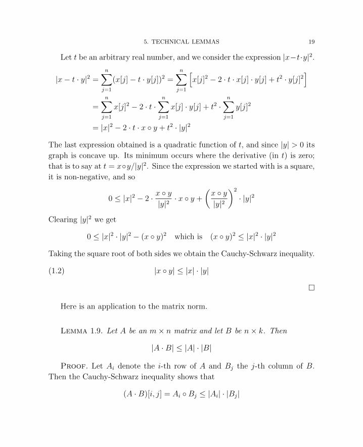
5. TECHNICAL LEMMAS 19

Let t be an arbitrary real number, and we consider the expression |x−t·y|2.

|x− t · y|2 =n∑

j=1

(x[j]− t · y[j])2 =n∑

j=1

[x[j]2 − 2 · t · x[j] · y[j] + t2 · y[j]2

]=

n∑j=1

x[j]2 − 2 · t ·n∑

j=1

x[j] · y[j] + t2 ·n∑

j=1

y[j]2

= |x|2 − 2 · t · x ◦ y + t2 · |y|2

The last expression obtained is a quadratic function of t, and since |y| > 0 its

graph is concave up. Its minimum occurs where the derivative (in t) is zero;

that is to say at t = x◦y/|y|2. Since the expression we started with is a square,

it is non-negative, and so

0 ≤ |x|2 − 2 · x ◦ y|y|2

· x ◦ y +

(x ◦ y|y|2

)2

· |y|2

Clearing |y|2 we get

0 ≤ |x|2 · |y|2 − (x ◦ y)2 which is (x ◦ y)2 ≤ |x|2 · |y|2

Taking the square root of both sides we obtain the Cauchy-Schwarz inequality.

(1.2) |x ◦ y| ≤ |x| · |y|

�

Here is an application to the matrix norm.

Lemma 1.9. Let A be an m× n matrix and let B be n× k. Then

|A ·B| ≤ |A| · |B|

Proof. Let Ai denote the i-th row of A and Bj the j-th column of B.

Then the Cauchy-Schwarz inequality shows that

(A ·B)[i, j] = Ai ◦Bj ≤ |Ai| · |Bj|

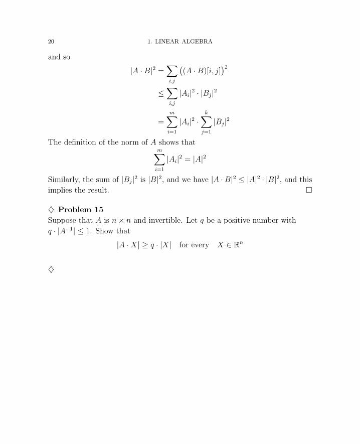
20 1. LINEAR ALGEBRA

and so

|A ·B|2 =∑i,j

((A ·B)[i, j]

)2≤∑i,j

|Ai|2 · |Bj|2

=m∑i=1

|Ai|2 ·k∑

j=1

|Bj|2

The definition of the norm of A shows thatm∑i=1

|Ai|2 = |A|2

Similarly, the sum of |Bj|2 is |B|2, and we have |A ·B|2 ≤ |A|2 · |B|2, and this

implies the result. �

♦ Problem 15

Suppose that A is n× n and invertible. Let q be a positive number with

q · |A−1| ≤ 1. Show that

|A ·X| ≥ q · |X| for every X ∈ Rn

♦

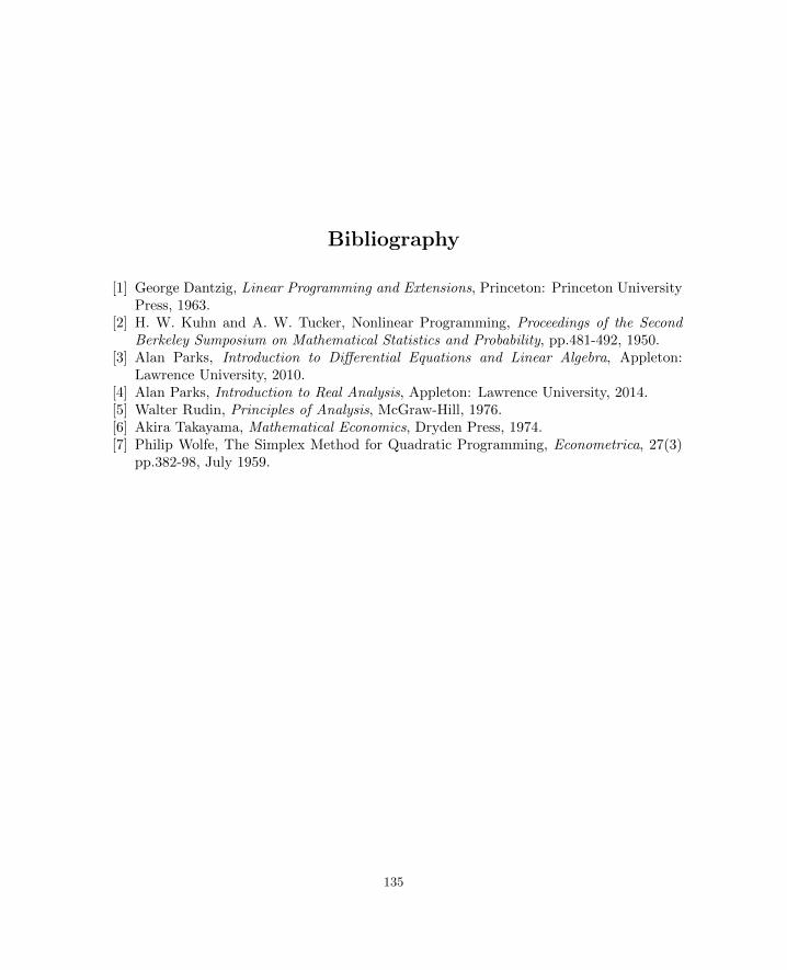
Bibliography

[1] George Dantzig, Linear Programming and Extensions, Princeton: Princeton UniversityPress, 1963.

[2] H. W. Kuhn and A. W. Tucker, Nonlinear Programming, Proceedings of the SecondBerkeley Sumposium on Mathematical Statistics and Probability, pp.481-492, 1950.

[3] Alan Parks, Introduction to Differential Equations and Linear Algebra, Appleton:Lawrence University, 2010.

[4] Alan Parks, Introduction to Real Analysis, Appleton: Lawrence University, 2014.[5] Walter Rudin, Principles of Analysis, McGraw-Hill, 1976.[6] Akira Takayama, Mathematical Economics, Dryden Press, 1974.[7] Philip Wolfe, The Simplex Method for Quadratic Programming, Econometrica, 27(3)

pp.382-98, July 1959.

135

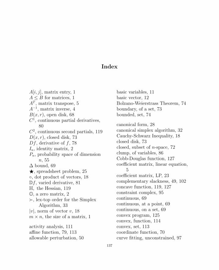
Index

A[i, j], matrix entry, 1A ≤ B for matrices, 1AT , matrix transpose, 5A−1, matrix inverse, 4B(x, r), open disk, 68C1, continuous partial derivatives,

80C2, continuous second partials, 119D(x, r), closed disk, 73Df , derivative of f , 78In, identity matrix, 2Pn, probability space of dimension

n, 55∆ bound, 69F, spreadsheet problem, 25◦, dot product of vectors, 18Df , varied derivative, 81H, the Hessian, 119O, a zero matrix, 2�, lex-top order for the Simplex

Algorithm, 33|v|, norm of vector v, 18m× n, the size of a matrix, 1

activity analysis, 111affine function, 79, 113allowable perturbation, 50

basic variables, 11basic vector, 12Bolzano-Weierstrass Theorem, 74boundary, of a set, 73bounded, set, 74

canonical form, 28canonical simplex algorithm, 32Cauchy-Schwarz Inequality, 18closed disk, 73closed, subset of n-space, 72clump, of variables, 86Cobb-Douglas function, 127coefficient matrix, linear equation,

5coefficient matrix, LP, 23complementary slackness, 49, 102concave function, 119, 127constraint complex, 95continuous, 69continuous, at a point, 69continuous, on a set, 69convex program, 125convex, function, 114convex, set, 113coordinate function, 70curve fitting, unconstrained, 97

137

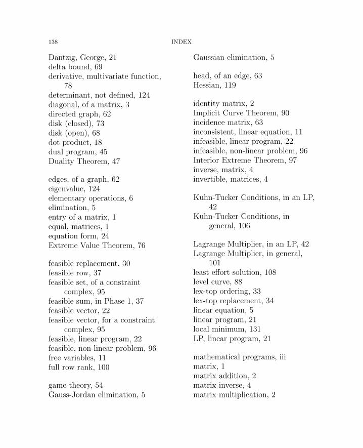
138 INDEX

Dantzig, George, 21delta bound, 69derivative, multivariate function,

78determinant, not defined, 124diagonal, of a matrix, 3directed graph, 62disk (closed), 73disk (open), 68dot product, 18dual program, 45Duality Theorem, 47

edges, of a graph, 62eigenvalue, 124elementary operations, 6elimination, 5entry of a matrix, 1equal, matrices, 1equation form, 24Extreme Value Theorem, 76

feasible replacement, 30feasible row, 37feasible set, of a constraint

complex, 95feasible sum, in Phase 1, 37feasible vector, 22feasible vector, for a constraint

complex, 95feasible, linear program, 22feasible, non-linear problem, 96free variables, 11full row rank, 100

game theory, 54Gauss-Jordan elimination, 5

Gaussian elimination, 5

head, of an edge, 63Hessian, 119

identity matrix, 2Implicit Curve Theorem, 90incidence matrix, 63inconsistent, linear equation, 11infeasible, linear program, 22infeasible, non-linear problem, 96Interior Extreme Theorem, 97inverse, matrix, 4invertible, matrices, 4

Kuhn-Tucker Conditions, in an LP,42

Kuhn-Tucker Conditions, ingeneral, 106

Lagrange Multiplier, in an LP, 42Lagrange Multiplier, in general,

101least effort solution, 108level curve, 88lex-top ordering, 33lex-top replacement, 34linear equation, 5linear program, 21local minimum, 131LP, linear program, 21

mathematical programs, iiimatrix, 1matrix addition, 2matrix inverse, 4matrix multiplication, 2

INDEX 139

matrix over a set, whose entriesare points, 81

matrix scalar multiplication, 2

non-degenerate, linear program, 32non-zero part, of a feasible point,

100norm, matrix, 18norm, vector, 18normal equations, 98

objective, iii, 21objective coefficient matrix, 23objective value, of canonical form,

28open disk, 68open, subset of n-space, 68

parameter, 23partial derivative, 77payoff matrix, 56payoff, of distributions, 56perturbation, 49Phase 1, 36Phase 2, 38positive definite, 131positive semi-definite, 122primal form, 23probability space, 55problem variables, 21product rule, 79production theory, 110

quadratic function, 79, 120quadratic program, 129

rank, 6Rank Theorem, 16

reduced form, 6reduced form, for an arbitrary

matrix, 9reducing matrix, 9regression line, 97replace, basic variable, 10replacement, basic variable, 10representing matrix, for an

elementary operation, 7resource bound, 49, 103right side matrix, 23right side, linear equation, 5

shadow price, 50, 105sign condition, 106Simplex Algorithm, 40size, of a matrix, 1slack variables, 24solution form, 30solution, linear program, 22solution, non-linear problem, 96special canonical form, for lex-top

ordering, 33square, matrix, 4squares error, 97standard segment, 113

tail, of an edge, 63theta ratio, 30transpose, 5Triangle Inequality, 67

utility function, 119, 128

varied derivative, of a function, 81vertices, of a graph, 62

140 INDEX

Wolfe’s Theorem for quadraticprograms, 129

Young’s inequality, 109

zero matrix, 2zero part, of a feasible point, 100zero sum, 56zero sum linear game, 54