Embed Size (px)
Citation preview
Introduction to Optimization
Introduction to Continuous Optimization III /Gradient-Based Algorithms
Dimo Brockhoff
INRIA Lille – Nord Europe
November 20, 2015
École Centrale Paris, Châtenay-Malabry, France
2Introduction to Optimization @ ECP, Nov. 20, 2015© Dimo Brockhoff, INRIA 2
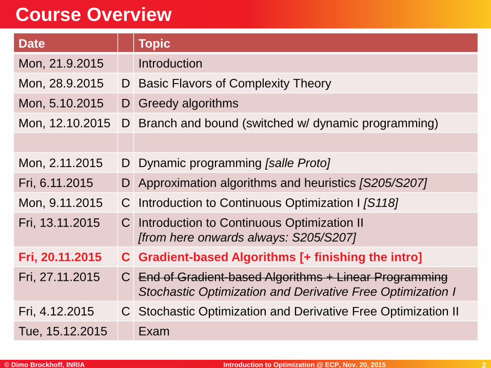
Date Topic
Mon, 21.9.2015 Introduction
Mon, 28.9.2015 D Basic Flavors of Complexity Theory
Mon, 5.10.2015 D Greedy algorithms
Mon, 12.10.2015 D Branch and bound (switched w/ dynamic programming)
Mon, 2.11.2015 D Dynamic programming [salle Proto]
Fri, 6.11.2015 D Approximation algorithms and heuristics [S205/S207]
Mon, 9.11.2015 C Introduction to Continuous Optimization I [S118]
Fri, 13.11.2015 C Introduction to Continuous Optimization II
[from here onwards always: S205/S207]
Fri, 20.11.2015 C Gradient-based Algorithms [+ finishing the intro]
Fri, 27.11.2015 C End of Gradient-based Algorithms + Linear Programming
Stochastic Optimization and Derivative Free Optimization I
Fri, 4.12.2015 C Stochastic Optimization and Derivative Free Optimization II
Tue, 15.12.2015 Exam
Course Overview
3Introduction to Optimization @ ECP, Nov. 20, 2015© Dimo Brockhoff, INRIA 3
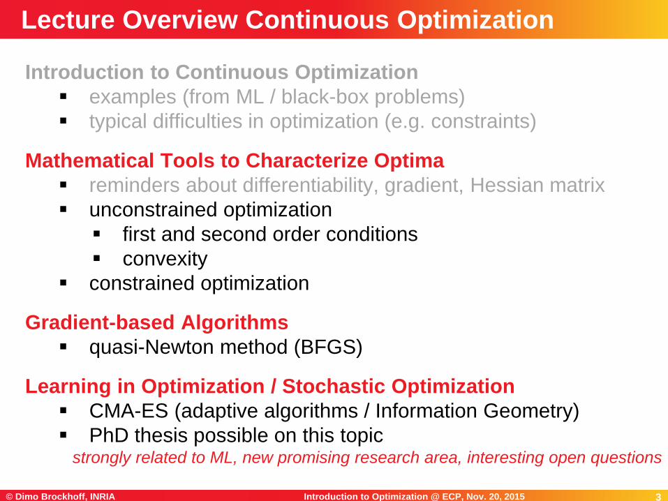
Introduction to Continuous Optimization
examples (from ML / black-box problems)
typical difficulties in optimization (e.g. constraints)
Mathematical Tools to Characterize Optima
reminders about differentiability, gradient, Hessian matrix
unconstrained optimization
first and second order conditions
convexity
constrained optimization
Gradient-based Algorithms
quasi-Newton method (BFGS)
Learning in Optimization / Stochastic Optimization
CMA-ES (adaptive algorithms / Information Geometry)
PhD thesis possible on this topicstrongly related to ML, new promising research area, interesting open questions
Lecture Overview Continuous Optimization
4Introduction to Optimization @ ECP, Nov. 20, 2015© Dimo Brockhoff, INRIA 4
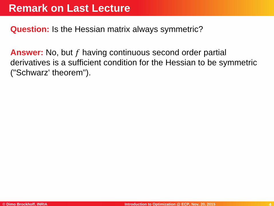
Question: Is the Hessian matrix always symmetric?
Answer: No, but 𝑓 having continuous second order partial
derivatives is a sufficient condition for the Hessian to be symmetric
("Schwarz' theorem").
Remark on Last Lecture
5Introduction to Optimization @ ECP, Nov. 20, 2015© Dimo Brockhoff, INRIA 5
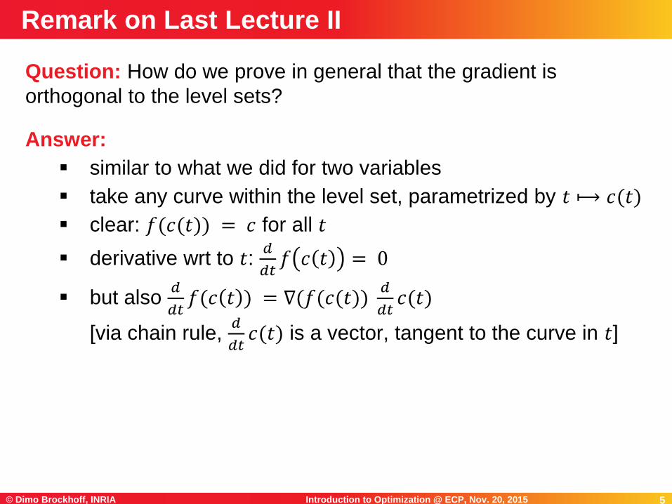
Question: How do we prove in general that the gradient is
orthogonal to the level sets?
Answer:
similar to what we did for two variables
take any curve within the level set, parametrized by 𝑡 ⟼ 𝑐(𝑡)
clear: 𝑓(𝑐(𝑡)) = 𝑐 for all 𝑡
derivative wrt to 𝑡: 𝑑
𝑑𝑡𝑓 𝑐 𝑡 = 0
but also 𝑑
𝑑𝑡𝑓(𝑐 𝑡 ) = ∇(𝑓(𝑐(𝑡))
𝑑
𝑑𝑡𝑐(𝑡)
[via chain rule, 𝑑
𝑑𝑡𝑐(𝑡) is a vector, tangent to the curve in 𝑡]
Remark on Last Lecture II

6Introduction to Optimization @ ECP, Nov. 20, 2015© Dimo Brockhoff, INRIA 6
Mathematical Tools to Characterize Optima
7Introduction to Optimization @ ECP, Nov. 20, 2015© Dimo Brockhoff, INRIA 7
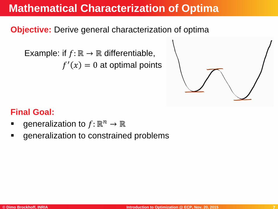
Objective: Derive general characterization of optima
Example: if 𝑓:ℝ → ℝ differentiable,
𝑓′ 𝑥 = 0 at optimal points
Final Goal:
generalization to 𝑓:ℝ𝑛 → ℝ
generalization to constrained problems
Mathematical Characterization of Optima

8Introduction to Optimization @ ECP, Nov. 20, 2015© Dimo Brockhoff, INRIA 8
Optimality Conditions
for Unconstrained Problems
9Introduction to Optimization @ ECP, Nov. 20, 2015© Dimo Brockhoff, INRIA 9
For 1-dimensional optimization problems 𝒇: ℝ → ℝ
Assume 𝑓 is differentiable
𝒙∗ is a local optimum ⟹ 𝑓′ 𝒙∗ = 0
not a sufficient condition: consider 𝑓 𝒙 = 𝒙3
proof via Taylor formula: 𝑓 𝒙∗ + 𝒉 = 𝑓 𝒙∗ + 𝑓′ 𝒙∗ 𝒉 + 𝑜(||𝒉||)
points 𝒚 such that 𝑓′ 𝒚 = 0 are called critical or stationary points
Generalization to 𝒏-dimensional functions
If 𝑓:𝑈 ⊂ ℝ𝑛 ⟼ ℝ is differentiable
necessary condition: If 𝒙∗ is a local optimum of 𝑓, then 𝛻𝑓 𝒙∗ = 𝟎
proof via Taylor formula
Optimality Conditions: First Order Necessary Cond.
10Introduction to Optimization @ ECP, Nov. 20, 2015© Dimo Brockhoff, INRIA 10
If 𝑓 is twice continuously differentiable
Necessary condition: if 𝒙∗ is a local minimum, then 𝛻𝑓 𝒙∗ = 0and 𝛻2𝑓(𝒙∗) is positive semi-definite
proof via Taylor formula at order 2
Sufficient condition: if 𝛻𝑓 𝒙∗ = 0 and 𝛻2𝑓 𝒙∗ is positive definite,
then 𝒙∗ is a strict local minimum
Proof of Sufficient Condition:
Let 𝜆 > 0 be the smallest eigenvalue of 𝛻2𝑓(𝒙∗), using a second
order Taylor expansion, we have for all 𝒉:
𝑓 𝒙∗ + 𝒉 − 𝑓 𝒙∗ = 𝛻𝑓 𝒙∗ 𝑇𝒉 +1
2𝒉𝑇𝛻2𝑓 𝒙∗ 𝒉 + 𝑜(||𝒉||2)
>𝜆
2| 𝒉 |2 + o(||𝒉||2) =
𝜆
2+𝑜(||𝒉||2)
||𝒉||2||𝒉||2
Second Order Necessary and Sufficient Opt. Cond.
11Introduction to Optimization @ ECP, Nov. 20, 2015© Dimo Brockhoff, INRIA 11
Let 𝑈 be a convex open set of ℝ𝑛 and 𝑓:𝑈 → ℝ. The function 𝑓 is
said to be convex if for all 𝒙, 𝒚 ∈ 𝑈 and for all 𝑡 ∈ [0,1]
𝑓 1 − 𝑡 𝒙 + 𝑡𝒚 ≤ 1 − 𝑡 𝑓 𝒙 + 𝑡𝑓(𝒚)
Theorem
If 𝑓 is differentiable, then 𝑓 is convex if and only if for all 𝒙, 𝒚
𝑓 𝒚 − 𝑓 𝒙 ≥ 𝛻𝑓 𝑥𝑇(𝒚 − 𝒙)
if 𝑛 = 1, the curve is on top of the tangent
If 𝑓 is twice continuously differentiable, then 𝑓 is convex if and only if
𝛻2𝑓(𝒙) is positive semi-definite for all 𝒙.
Convex Functions
12Introduction to Optimization @ ECP, Nov. 20, 2015© Dimo Brockhoff, INRIA 12
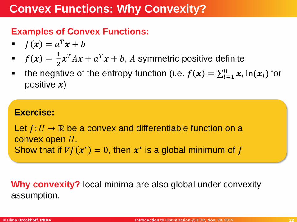
Examples of Convex Functions:
𝑓 𝒙 = 𝑎𝑇𝒙 + 𝑏
𝑓 𝒙 =1
2𝒙𝑇𝐴𝒙 + 𝑎𝑇𝒙 + 𝑏, 𝐴 symmetric positive definite
the negative of the entropy function (i.e. 𝑓 𝒙 = 𝑖=1𝑛 𝒙𝑖 ln(𝒙𝒊) for
positive 𝒙)
Why convexity? local minima are also global under convexity
assumption.
Convex Functions: Why Convexity?
Exercise:
Let 𝑓:𝑈 → ℝ be a convex and differentiable function on a
convex open 𝑈.
Show that if 𝛻𝑓 𝒙∗ = 0, then 𝒙∗ is a global minimum of 𝑓

13Introduction to Optimization @ ECP, Nov. 20, 2015© Dimo Brockhoff, INRIA 13
Constrained Optimization
14Introduction to Optimization @ ECP, Nov. 20, 2015© Dimo Brockhoff, INRIA 14
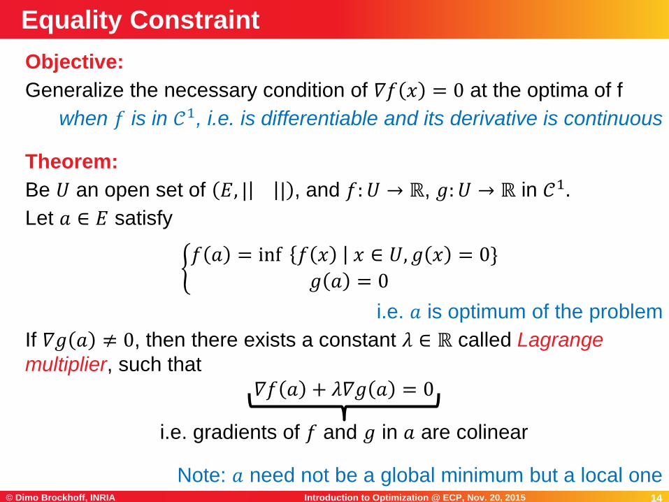
Objective:
Generalize the necessary condition of 𝛻𝑓 𝑥 = 0 at the optima of f
when 𝑓 is in 𝒞1, i.e. is differentiable and its derivative is continuous
Theorem:
Be 𝑈 an open set of 𝐸, | | , and 𝑓: 𝑈 → ℝ, 𝑔:𝑈 → ℝ in 𝒞1.
Let 𝑎 ∈ 𝐸 satisfy
𝑓 𝑎 = inf 𝑓 𝑥 𝑥 ∈ 𝑈, 𝑔 𝑥 = 0}
𝑔 𝑎 = 0
i.e. 𝑎 is optimum of the problem
If 𝛻𝑔 𝑎 ≠ 0, then there exists a constant 𝜆 ∈ ℝ called Lagrange
multiplier, such that
𝛻𝑓 𝑎 + 𝜆𝛻𝑔 𝑎 = 0
i.e. gradients of 𝑓 and 𝑔 in 𝑎 are colinear
Note: 𝑎 need not be a global minimum but a local one
Equality Constraint
15Introduction to Optimization @ ECP, Nov. 20, 2015© Dimo Brockhoff, INRIA 15
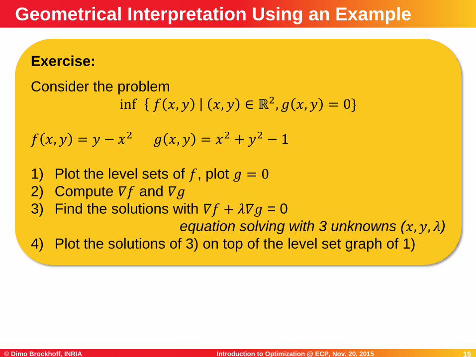
Geometrical Interpretation Using an Example
Exercise:
Consider the problem
inf 𝑓 𝑥, 𝑦 𝑥, 𝑦 ∈ ℝ2, 𝑔 𝑥, 𝑦 = 0}
𝑓 𝑥, 𝑦 = 𝑦 − 𝑥2 𝑔 𝑥, 𝑦 = 𝑥2 + 𝑦2 − 1
1) Plot the level sets of 𝑓, plot 𝑔 = 02) Compute 𝛻𝑓 and 𝛻𝑔3) Find the solutions with 𝛻𝑓 + 𝜆𝛻𝑔 = 0
equation solving with 3 unknowns (𝑥, 𝑦, 𝜆)
4) Plot the solutions of 3) on top of the level set graph of 1)
17Introduction to Optimization @ ECP, Nov. 20, 2015© Dimo Brockhoff, INRIA 17
Intuitive way to retrieve the Euler-Lagrange equation:
In a local minimum 𝑎 of a constrained problem, the
hypersurfaces (or level sets) 𝑓 = 𝑓(𝑎) and 𝑔 = 0 are necessarily
tangent (otherwise we could decrease 𝑓 by moving along 𝑔 = 0).
Since the gradients 𝛻𝑓 𝑎 and 𝛻𝑔(𝑎) are orthogonal to the level
sets 𝑓 = 𝑓(𝑎) and 𝑔 = 0, it follows that 𝛻𝑓(𝑎) and 𝛻𝑔(𝑎) are
colinear.
Interpretation of Euler-Lagrange Equation
18Introduction to Optimization @ ECP, Nov. 20, 2015© Dimo Brockhoff, INRIA 18
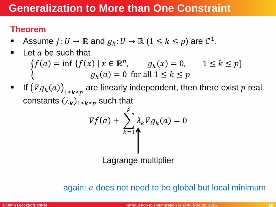
Theorem
Assume 𝑓:𝑈 → ℝ and 𝑔𝑘: 𝑈 → ℝ (1 ≤ 𝑘 ≤ 𝑝) are 𝒞1.
Let 𝑎 be such that
𝑓 𝑎 = inf 𝑓 𝑥 𝑥 ∈ ℝ𝑛, 𝑔𝑘 𝑥 = 0, 1 ≤ 𝑘 ≤ 𝑝}
𝑔𝑘 𝑎 = 0 for all 1 ≤ 𝑘 ≤ 𝑝
If 𝛻𝑔𝑘 𝑎1≤𝑘≤𝑝
are linearly independent, then there exist 𝑝 real
constants 𝜆𝑘 1≤𝑘≤𝑝 such that
𝛻𝑓 𝑎 +
𝑘=1
𝑝
𝜆𝑘𝛻𝑔𝑘 𝑎 = 0
again: 𝑎 does not need to be global but local minimum
Generalization to More than One Constraint
Lagrange multiplier
19Introduction to Optimization @ ECP, Nov. 20, 2015© Dimo Brockhoff, INRIA 19
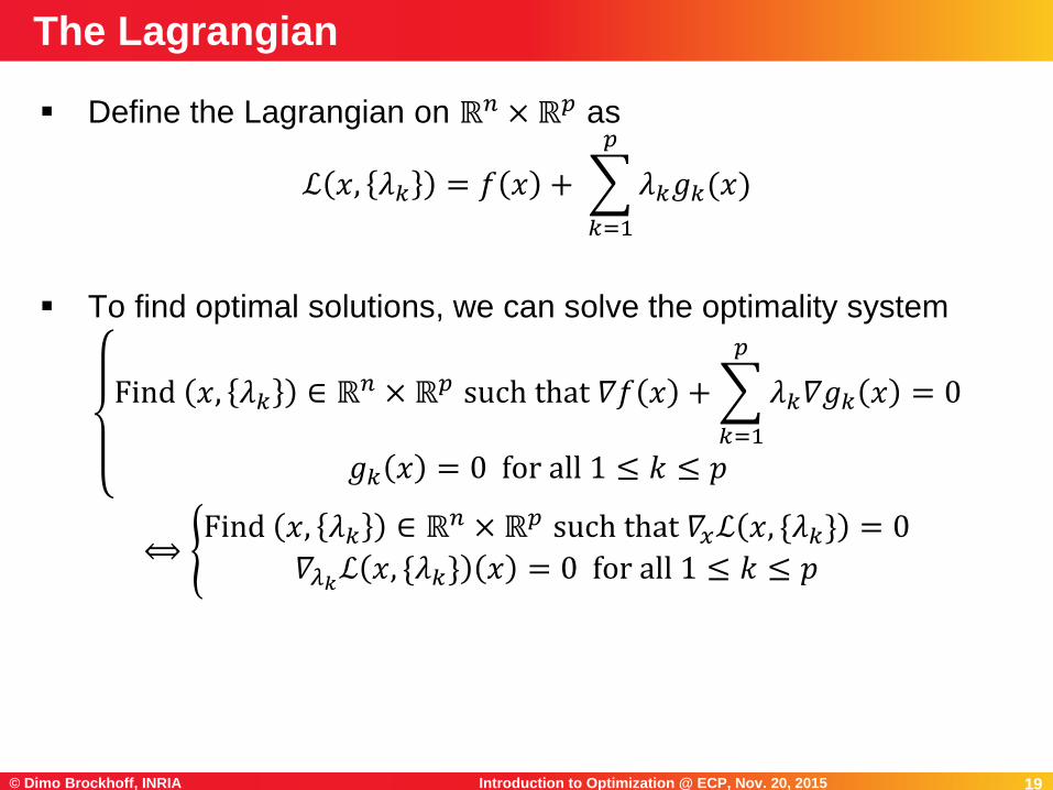
Define the Lagrangian on ℝ𝑛 × ℝ𝑝 as
ℒ 𝑥, 𝜆𝑘 = 𝑓 𝑥 +
𝑘=1
𝑝
𝜆𝑘𝑔𝑘(𝑥)
To find optimal solutions, we can solve the optimality system
Find 𝑥, 𝜆𝑘 ∈ ℝ𝑛 × ℝ𝑝 such that 𝛻𝑓 𝑥 +
𝑘=1
𝑝
𝜆𝑘𝛻𝑔𝑘 𝑥 = 0
𝑔𝑘 𝑥 = 0 for all 1 ≤ 𝑘 ≤ 𝑝
⟺ Find 𝑥, 𝜆𝑘 ∈ ℝ𝑛 × ℝ𝑝 such that 𝛻𝑥ℒ 𝑥, {𝜆𝑘} = 0
𝛻𝜆𝑘ℒ 𝑥, {𝜆𝑘} 𝑥 = 0 for all 1 ≤ 𝑘 ≤ 𝑝
The Lagrangian
20Introduction to Optimization @ ECP, Nov. 20, 2015© Dimo Brockhoff, INRIA 20
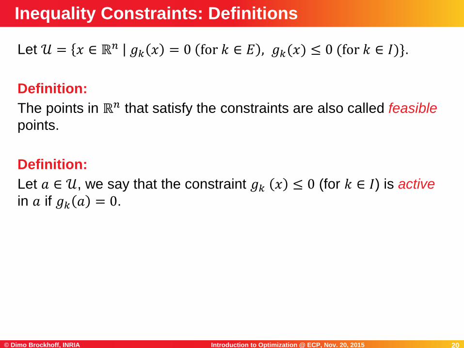
Let 𝒰 = 𝑥 ∈ ℝ𝑛 𝑔𝑘 𝑥 = 0 for 𝑘 ∈ 𝐸 , 𝑔𝑘(𝑥) ≤ 0 (for 𝑘 ∈ 𝐼)}.
Definition:
The points in ℝ𝑛 that satisfy the constraints are also called feasible
points.
Definition:
Let 𝑎 ∈ 𝒰, we say that the constraint 𝑔𝑘 𝑥 ≤ 0 (for 𝑘 ∈ 𝐼) is active
in 𝑎 if 𝑔𝑘 𝑎 = 0.
Inequality Constraints: Definitions
21Introduction to Optimization @ ECP, Nov. 20, 2015© Dimo Brockhoff, INRIA 21
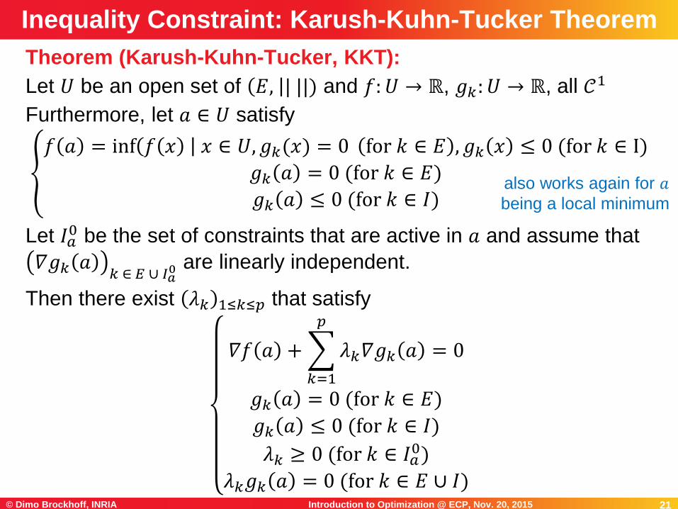
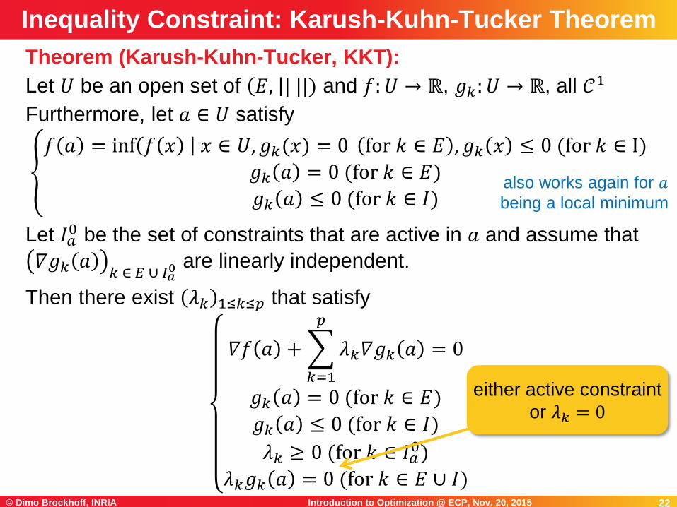
Theorem (Karush-Kuhn-Tucker, KKT):
Let 𝑈 be an open set of 𝐸, | ||) and 𝑓: 𝑈 → ℝ, 𝑔𝑘: 𝑈 → ℝ, all 𝒞1
Furthermore, let 𝑎 ∈ 𝑈 satisfy
𝑓 𝑎 = inf 𝑓 𝑥 𝑥 ∈ 𝑈, 𝑔𝑘(𝑥) = 0 for 𝑘 ∈ 𝐸 , 𝑔𝑘 𝑥 ≤ 0 (for 𝑘 ∈ I)
𝑔𝑘 𝑎 = 0 (for 𝑘 ∈ 𝐸)
𝑔𝑘 𝑎 ≤ 0 (for 𝑘 ∈ 𝐼)
Let 𝐼𝑎0 be the set of constraints that are active in 𝑎 and assume that
𝛻𝑔𝑘 𝑎𝑘 ∈ 𝐸 ∪ 𝐼𝑎
0 are linearly independent.
Then there exist 𝜆𝑘 1≤𝑘≤𝑝 that satisfy
𝛻𝑓 𝑎 +
𝑘=1
𝑝
𝜆𝑘𝛻𝑔𝑘 𝑎 = 0
𝑔𝑘 𝑎 = 0 (for 𝑘 ∈ 𝐸)
𝑔𝑘 𝑎 ≤ 0 (for 𝑘 ∈ 𝐼)
𝜆𝑘 ≥ 0 (for 𝑘 ∈ 𝐼𝑎0)
𝜆𝑘𝑔𝑘 𝑎 = 0 (for 𝑘 ∈ 𝐸 ∪ 𝐼)
Inequality Constraint: Karush-Kuhn-Tucker Theorem
also works again for 𝑎being a local minimum
22Introduction to Optimization @ ECP, Nov. 20, 2015© Dimo Brockhoff, INRIA 22
Theorem (Karush-Kuhn-Tucker, KKT):
Let 𝑈 be an open set of 𝐸, | ||) and 𝑓: 𝑈 → ℝ, 𝑔𝑘: 𝑈 → ℝ, all 𝒞1
Furthermore, let 𝑎 ∈ 𝑈 satisfy
𝑓 𝑎 = inf 𝑓 𝑥 𝑥 ∈ 𝑈, 𝑔𝑘(𝑥) = 0 for 𝑘 ∈ 𝐸 , 𝑔𝑘 𝑥 ≤ 0 (for 𝑘 ∈ I)
𝑔𝑘 𝑎 = 0 (for 𝑘 ∈ 𝐸)
𝑔𝑘 𝑎 ≤ 0 (for 𝑘 ∈ 𝐼)
Let 𝐼𝑎0 be the set of constraints that are active in 𝑎 and assume that
𝛻𝑔𝑘 𝑎𝑘 ∈ 𝐸 ∪ 𝐼𝑎
0 are linearly independent.
Then there exist 𝜆𝑘 1≤𝑘≤𝑝 that satisfy
𝛻𝑓 𝑎 +
𝑘=1
𝑝
𝜆𝑘𝛻𝑔𝑘 𝑎 = 0
𝑔𝑘 𝑎 = 0 (for 𝑘 ∈ 𝐸)
𝑔𝑘 𝑎 ≤ 0 (for 𝑘 ∈ 𝐼)
𝜆𝑘 ≥ 0 (for 𝑘 ∈ 𝐼𝑎0)
𝜆𝑘𝑔𝑘 𝑎 = 0 (for 𝑘 ∈ 𝐸 ∪ 𝐼)
Inequality Constraint: Karush-Kuhn-Tucker Theorem
also works again for 𝑎being a local minimum
either active constraint
or 𝜆𝑘 = 0
23Introduction to Optimization @ ECP, Nov. 20, 2015© Dimo Brockhoff, INRIA 23
Descent Methods
24Introduction to Optimization @ ECP, Nov. 20, 2015© Dimo Brockhoff, INRIA 24
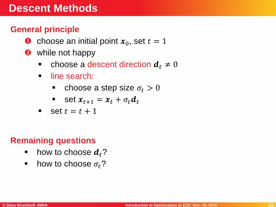
General principle
choose an initial point 𝒙0, set 𝑡 = 1
while not happy
choose a descent direction 𝒅𝑡 ≠ 0
line search:
choose a step size 𝜎𝑡 > 0
set 𝒙𝑡+1 = 𝒙𝑡 + 𝜎𝑡𝒅𝑡
set 𝑡 = 𝑡 + 1
Remaining questions
how to choose 𝒅𝑡?
how to choose 𝜎𝑡?
Descent Methods
25Introduction to Optimization @ ECP, Nov. 20, 2015© Dimo Brockhoff, INRIA 25
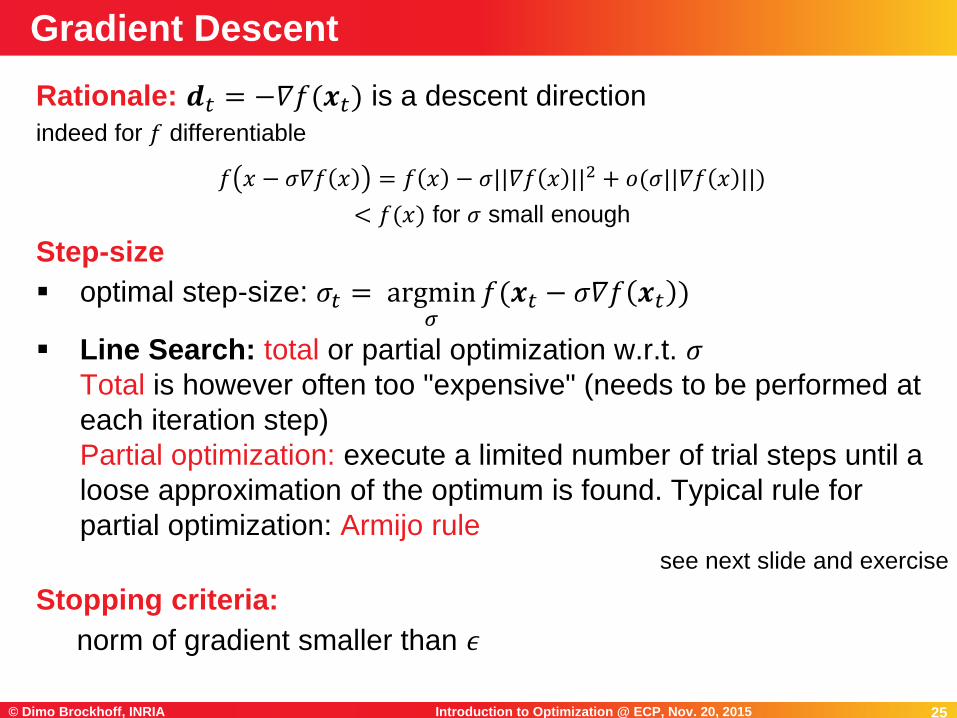
Rationale: 𝒅𝑡 = −𝛻𝑓(𝒙𝑡) is a descent direction
indeed for 𝑓 differentiable
𝑓 𝑥 − 𝜎𝛻𝑓 𝑥 = 𝑓 𝑥 − 𝜎||𝛻𝑓 𝑥 ||2 + 𝑜(𝜎||𝛻𝑓 𝑥 ||)
< 𝑓(𝑥) for 𝜎 small enough
Step-size
optimal step-size: 𝜎𝑡 = argmin𝜎
𝑓(𝒙𝑡 − 𝜎𝛻𝑓 𝒙𝑡 )
Line Search: total or partial optimization w.r.t. 𝜎Total is however often too "expensive" (needs to be performed at
each iteration step)
Partial optimization: execute a limited number of trial steps until a
loose approximation of the optimum is found. Typical rule for
partial optimization: Armijo rulesee next slide and exercise
Stopping criteria:
norm of gradient smaller than 𝜖
Gradient Descent
26Introduction to Optimization @ ECP, Nov. 20, 2015© Dimo Brockhoff, INRIA 26
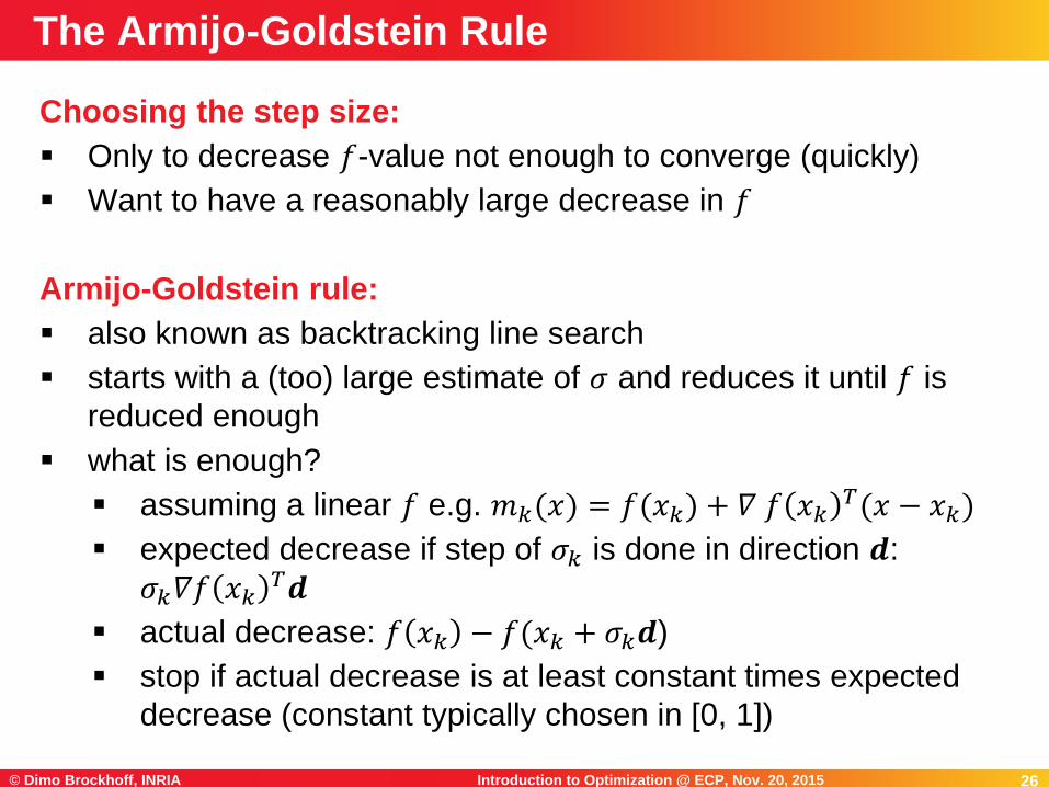
Choosing the step size:
Only to decrease 𝑓-value not enough to converge (quickly)
Want to have a reasonably large decrease in 𝑓
Armijo-Goldstein rule:
also known as backtracking line search
starts with a (too) large estimate of 𝜎 and reduces it until 𝑓 is
reduced enough
what is enough?
assuming a linear 𝑓 e.g. 𝑚𝑘(𝑥) = 𝑓(𝑥𝑘) + 𝛻 𝑓 𝑥𝑘𝑇(𝑥 − 𝑥𝑘)
expected decrease if step of 𝜎𝑘 is done in direction 𝒅:
𝜎𝑘𝛻𝑓 𝑥𝑘𝑇𝒅
actual decrease: 𝑓 𝑥𝑘 − 𝑓(𝑥𝑘 + 𝜎𝑘𝒅)
stop if actual decrease is at least constant times expected
decrease (constant typically chosen in [0, 1])
The Armijo-Goldstein Rule
27Introduction to Optimization @ ECP, Nov. 20, 2015© Dimo Brockhoff, INRIA 27
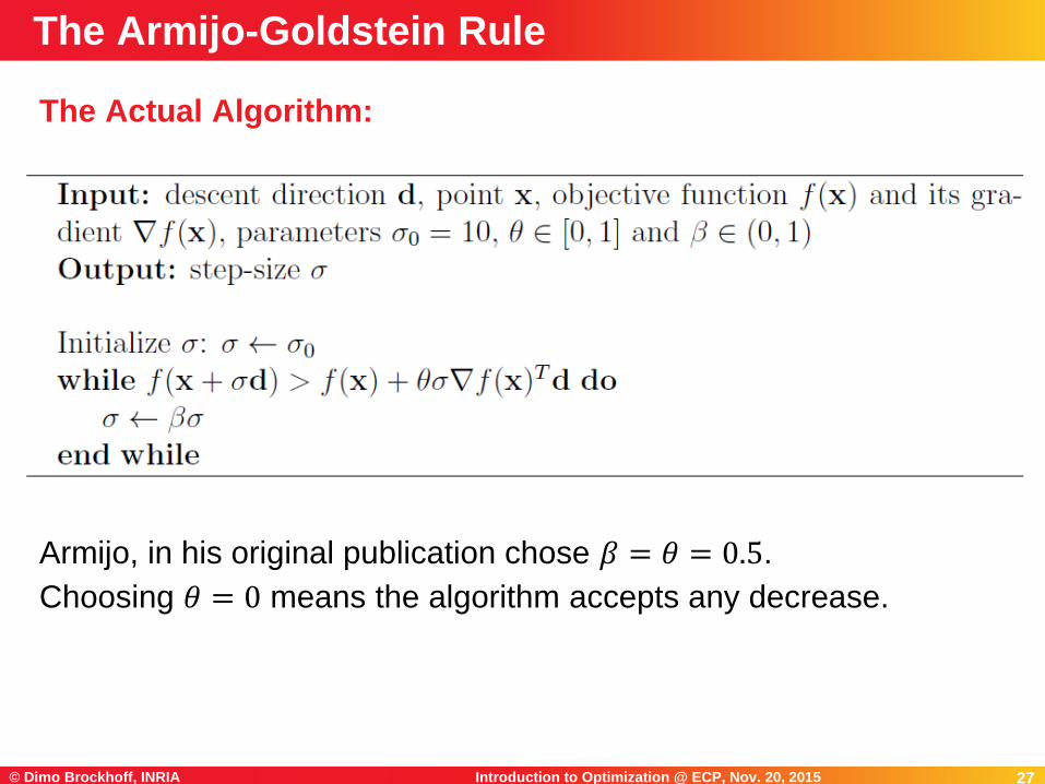
The Actual Algorithm:
Armijo, in his original publication chose 𝛽 = 𝜃 = 0.5.
Choosing 𝜃 = 0 means the algorithm accepts any decrease.
The Armijo-Goldstein Rule
28Introduction to Optimization @ ECP, Nov. 20, 2015© Dimo Brockhoff, INRIA 28
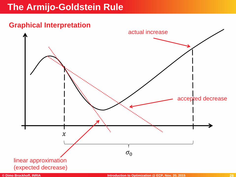
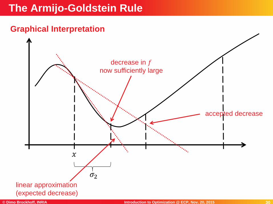
Graphical Interpretation
The Armijo-Goldstein Rule
𝑥
𝜎0linear approximation
(expected decrease)
accepted decrease
actual increase
29Introduction to Optimization @ ECP, Nov. 20, 2015© Dimo Brockhoff, INRIA 29
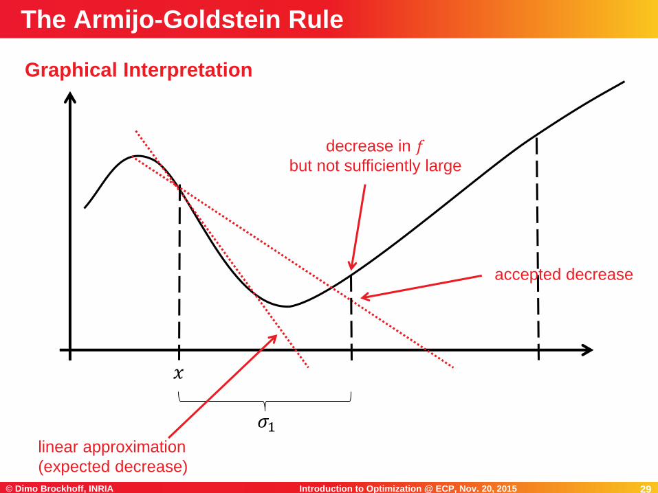
Graphical Interpretation
The Armijo-Goldstein Rule
𝑥
𝜎1linear approximation
(expected decrease)
accepted decrease
decrease in 𝑓but not sufficiently large
30Introduction to Optimization @ ECP, Nov. 20, 2015© Dimo Brockhoff, INRIA 30
Graphical Interpretation
The Armijo-Goldstein Rule
𝑥
𝜎2linear approximation
(expected decrease)
accepted decrease
decrease in 𝑓now sufficiently large
31Introduction to Optimization @ ECP, Nov. 20, 2015© Dimo Brockhoff, INRIA 31
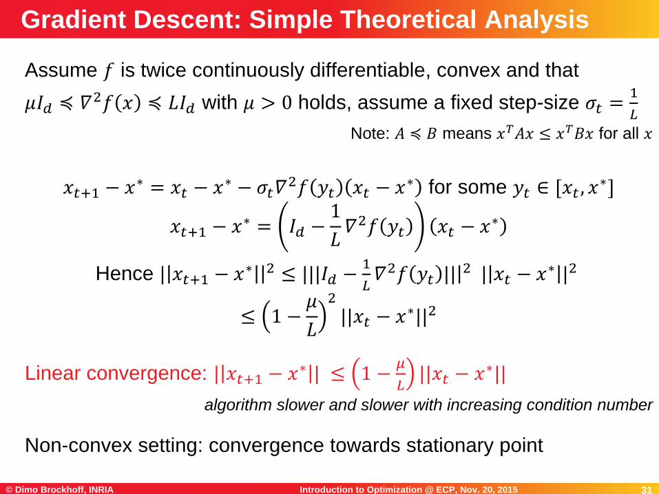
Assume 𝑓 is twice continuously differentiable, convex and that
𝜇𝐼𝑑 ≼ 𝛻2𝑓 𝑥 ≼ 𝐿𝐼𝑑 with 𝜇 > 0 holds, assume a fixed step-size 𝜎𝑡 =1
𝐿
Note: 𝐴 ≼ 𝐵 means 𝑥𝑇𝐴𝑥 ≤ 𝑥𝑇𝐵𝑥 for all 𝑥
𝑥𝑡+1 − 𝑥∗ = 𝑥𝑡 − 𝑥∗ − 𝜎𝑡𝛻2𝑓 𝑦𝑡 𝑥𝑡 − 𝑥∗ for some 𝑦𝑡 ∈ [𝑥𝑡 , 𝑥
∗]
𝑥𝑡+1 − 𝑥∗ = 𝐼𝑑 −1
𝐿𝛻2𝑓 𝑦𝑡 𝑥𝑡 − 𝑥∗
Hence | 𝑥𝑡+1 − 𝑥∗ |2 ≤ |||𝐼𝑑 −1
𝐿𝛻2𝑓 𝑦𝑡 |||2 | 𝑥𝑡 − 𝑥∗ |2
≤ 1 −𝜇
𝐿
2
||𝑥𝑡 − 𝑥∗||2
Linear convergence: | 𝑥𝑡+1 − 𝑥∗ | ≤ 1 −𝜇
𝐿||𝑥𝑡 − 𝑥∗||
algorithm slower and slower with increasing condition number
Non-convex setting: convergence towards stationary point
Gradient Descent: Simple Theoretical Analysis
32Introduction to Optimization @ ECP, Nov. 20, 2015© Dimo Brockhoff, INRIA 32
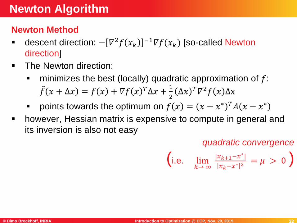
Newton Method
descent direction: − 𝛻2𝑓 𝑥𝑘−1𝛻𝑓(𝑥𝑘) [so-called Newton
direction]
The Newton direction:
minimizes the best (locally) quadratic approximation of 𝑓:
𝑓 𝑥 + Δ𝑥 = 𝑓 𝑥 + 𝛻𝑓 𝑥 𝑇Δ𝑥 +1
2Δ𝑥 𝑇𝛻2𝑓 𝑥 Δx
points towards the optimum on 𝑓 𝑥 = 𝑥 − 𝑥∗ 𝑇𝐴 𝑥 − 𝑥∗
however, Hessian matrix is expensive to compute in general and
its inversion is also not easy
quadratic convergence
(i.e. lim𝑘→∞
|𝑥𝑘+1−𝑥∗|
𝑥𝑘−𝑥∗ 2 = 𝜇 > 0 )
Newton Algorithm
33Introduction to Optimization @ ECP, Nov. 20, 2015© Dimo Brockhoff, INRIA 33
Affine Invariance: same behavior on 𝑓 𝑥 and 𝑓(𝐴𝑥 + 𝑏) for 𝐴 ∈GLn(ℝ)
Newton method is affine invariantsee http://users.ece.utexas.edu/~cmcaram/EE381V_2012F/
Lecture_6_Scribe_Notes.final.pdf
same convergence rate on all convex-quadratic functions
Gradient method not affine invariant
Remark: Affine Invariance
34Introduction to Optimization @ ECP, Nov. 20, 2015© Dimo Brockhoff, INRIA 34
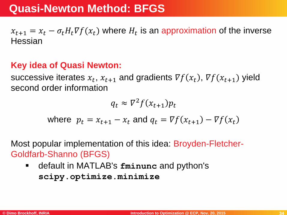
𝑥𝑡+1 = 𝑥𝑡 − 𝜎𝑡𝐻𝑡𝛻𝑓(𝑥𝑡) where 𝐻𝑡 is an approximation of the inverse
Hessian
Key idea of Quasi Newton:
successive iterates 𝑥𝑡, 𝑥𝑡+1 and gradients 𝛻𝑓 𝑥𝑡 , 𝛻𝑓(𝑥𝑡+1) yield
second order information
𝑞𝑡 ≈ 𝛻2𝑓 𝑥𝑡+1 𝑝𝑡
where 𝑝𝑡 = 𝑥𝑡+1 − 𝑥𝑡 and 𝑞𝑡 = 𝛻𝑓 𝑥𝑡+1 − 𝛻𝑓 𝑥𝑡
Most popular implementation of this idea: Broyden-Fletcher-
Goldfarb-Shanno (BFGS)
default in MATLAB's fminunc and python's
scipy.optimize.minimize
Quasi-Newton Method: BFGS
35Introduction to Optimization @ ECP, Nov. 20, 2015© Dimo Brockhoff, INRIA 35
I hope it became clear...
...what are gradient and Hessian
...what are sufficient and necessary conditions for optimality
...what is the difference between gradient and Newton direction
...and that adapting the step size in descent algorithms is crucial.
Conclusions