Embed Size (px)
Citation preview
INTRODUCTION TO NONLINEAR PARTIAL DIFFERENTIAL
EQUATIONS
J. BanasiakSchool of Mathematical Sciences
University of KwaZulu-Natal, Durban, South Africa

2
Contents
1 Origins of partial differential equations 5
1 Basic facts from Calculus . . . . . . . . . . . . . . . . . . . . . . . . . . . . . . . . . . . . . . 5
2 Conservation laws . . . . . . . . . . . . . . . . . . . . . . . . . . . . . . . . . . . . . . . . . . 13
2.1 One-dimensional conservation law . . . . . . . . . . . . . . . . . . . . . . . . . . . . . 13
2.2 Conservation laws in higher dimensions . . . . . . . . . . . . . . . . . . . . . . . . . . 16
3 Constitutive relations and examples . . . . . . . . . . . . . . . . . . . . . . . . . . . . . . . . 17
3.1 Transport equation . . . . . . . . . . . . . . . . . . . . . . . . . . . . . . . . . . . . . . 17
3.2 McKendrick partial differential equation . . . . . . . . . . . . . . . . . . . . . . . . . . 17
3.3 Diffusion/heat equations . . . . . . . . . . . . . . . . . . . . . . . . . . . . . . . . . . . 18
3.4 Variations of diffusion equation . . . . . . . . . . . . . . . . . . . . . . . . . . . . . . . 19
2 First order linear partial differential equations 21
1 Basic theory and examples . . . . . . . . . . . . . . . . . . . . . . . . . . . . . . . . . . . . . . 21
1.1 The McKendrick equation . . . . . . . . . . . . . . . . . . . . . . . . . . . . . . . . . . 28
3 First order nonlinear equations 31
1 Basic theory . . . . . . . . . . . . . . . . . . . . . . . . . . . . . . . . . . . . . . . . . . . . . . 31
2 Application to traffic flow . . . . . . . . . . . . . . . . . . . . . . . . . . . . . . . . . . . . . . 46
3 An exactly solvable McKendrick nonlinear model . . . . . . . . . . . . . . . . . . . . . . . . . 52
4 Similarity methods for linear and non-linear diffusion 57
1 Similarity method . . . . . . . . . . . . . . . . . . . . . . . . . . . . . . . . . . . . . . . . . . 57
2 Linear diffusion equation . . . . . . . . . . . . . . . . . . . . . . . . . . . . . . . . . . . . . . . 59
3 Nonlinear diffusion models . . . . . . . . . . . . . . . . . . . . . . . . . . . . . . . . . . . . . . 61
3.1 Models . . . . . . . . . . . . . . . . . . . . . . . . . . . . . . . . . . . . . . . . . . . . 61
3.2 Some solutions . . . . . . . . . . . . . . . . . . . . . . . . . . . . . . . . . . . . . . . . 62
5 Travelling waves 71
1 Introduction . . . . . . . . . . . . . . . . . . . . . . . . . . . . . . . . . . . . . . . . . . . . . . 71
2 Basic examples . . . . . . . . . . . . . . . . . . . . . . . . . . . . . . . . . . . . . . . . . . . . 72
3

4 CONTENTS
3 The Burger equation . . . . . . . . . . . . . . . . . . . . . . . . . . . . . . . . . . . . . . . . . 73
3.1 Travelling wave solutions . . . . . . . . . . . . . . . . . . . . . . . . . . . . . . . . . . 73
3.2 The Cole-Hopf transformation and analytic solution to the Burgers equation . . . . . 74
4 The Korteweg-de Vries equation and solitons . . . . . . . . . . . . . . . . . . . . . . . . . . . 77
5 The Fisher equation . . . . . . . . . . . . . . . . . . . . . . . . . . . . . . . . . . . . . . . . . 79
5.1 An explicit travelling wave solution to the Fisher equation . . . . . . . . . . . . . . . . 82
6 The Nagumo equation . . . . . . . . . . . . . . . . . . . . . . . . . . . . . . . . . . . . . . . . 83

Chapter 1
Origins of partial differentialequations
1 Basic facts from Calculus
In the course we shall frequently need several facts from the integration theory. We list them here as theorems,though we shall not prove them during the lecture. Some easier proofs should be done as exercises.
Theorem 1.1 Let f be a continuous function in Ω, where Ω ⊂ Rd is a bounded domain. Assume that∀x∈Ω f(x) ≥ 0 and
∫Ω
f(x)dx = 0. Then f ≡ 0 in Ω.
Another ”vanishing function” theorem reads as follows.
Theorem 1.2 Let f be a continuous function in a domain Ω such that∫Ω0
f(x)dx = 0 for any Ω0 ⊂ Ω.
Then f ≡ 0 in Ω.
In the proofs of both theorems the crucial role is played by the theorem on local sign preservation bycontinuous functions: if f is continuous at x0 and f(x0) > 0, then there exists a ball centered at x0 suchf(x) > 0 for x from this ball.
Next we shall consider perhaps the most important theorem of multidimensional integral calculus which isGreen’s-Gauss’-Divergence-.... Theorem. Before entering into details, however, we shall devote some timeto the geometry of domains in space.
In one-dimensional space R1 typical sets with which we will be concerned are open intervals ]a, b[, where−∞ ≤ a < b ≤ +∞. For −∞ < a < b < +∞, by [a, b] we will denote the closed interval with endpointsa, b. In this case, we say that ]a, b[ is the interior of the interval, [a, b] is its closure and the two-point setconsisting of a and b constitutes the boundary.
In general, for a set Ω, we denote by ∂Ω its boundary.
The situation in R2 and R3 is much more complicated. Let us consider first the two-dimensional situation.Then, in most cases, the boundary ∂Ω of a two-dimensional region Ω is a closed curve. The two most usedanalytic descriptions of curves in R2 are:
a) as a level curve of a function of two variables
F (x1, x2) = c,
5
6 CHAPTER 1. ORIGINS OF PARTIAL DIFFERENTIAL EQUATIONS
b) using two functions of a single variable
x1(t) = f(t),x2(t) = g(t),
where t ∈ [t0, t1] (parametric description). Note that since the curve is to be closed, we must havef(t0) = f(t1) and g(t0) = g(t1).
In many cases the boundary is composed of a number of arcs so that it is impossible to give a single analyticaldescription applicable to the whole boundary.
Example 1.1 Let us consider the elliptical region x21/a2 + x2
2/b2 ≤ 1. The boundary is then the ellipse
x21
a2+
x22
b2= 1.
This is the description of the curve (ellipse) as a level curve of the function F (x1, x2) = x21/a2 + x2
2/b2 (withthe constant c = 1). Equivalently, the boundary can be written in parametric form as
x1(t) = a cos t, x2(t) = b sin t,
with t ∈ [0, 2π].
In three dimensions the boundary of a solid Ω is a two-dimensional surface. This surface can be analyticallydescribed as a level surface of a function of three variables
F (x1, x2, x3) = c,
or parametrically by, this time, three functions of two variables each:
x1(t, s) = f(t, s),x2(t, s) = g(t, s),x3(t, s) = h(t, s), t ∈ [t0, t1], s ∈ [s0, s1].
As in two dimensions, it is possible that the boundary is made up of several patches having different analyticdescriptions.
Example 1.2 Consider the domain Ω bounded by the ellipsoid
x21
a2+
x22
b2+
x23
c2= 1.
The boundary here is directly given as the level surface of the function F (x1, x2, x3) = x21/a2 +x2
2/b2 +x23/c2:
F (x1, x2, x3) = 1.
The same boundary can be described parametrically as r(t, s) = (f(t, s), g(t, s), h(t, s)), where
f(t, s) = a cos t sin s
g(t, s) = b sin t sin s
h(t, s) = c cos s
where t ∈ [0, 2π], s ∈ [0, π].
1. BASIC FACTS FROM CALCULUS 7
One of the most important concepts in partial differential equations is that of the unit outward normal vectorto the boundary of the set. For a given point p ∈ ∂Ω this is the vector n, normal (perpendicular) to theboundary at p, pointing outside Ω, and having unit length.
If the boundary of (two or three dimensional) set Ω is given as a level curve of a function F , then the vectorgiven by
N(p) = ∇F |p,
is normal to the boundary at p. However, it is not necessarily unit, nor outward. To make it a unit vector,we divide N by its length; then the unit outward normal is either n = N/‖N‖, or n = −N/‖N‖ and theproper sign must be selected by inspection.
Example 1.3 Find the unit outward normal to the ellipsoid
x21 +
x22
4+
x23
9= 1,
at the point p = (1/√
2, 0, 3/√
2).
Since F (x1, x2, x3) = x21 + x2
24 + x2
39 , we obtain ∇F = (2x1, x2/2, 2x3/9). Therefore
N(p) = ∇F |p = (2/√
2, 0, 2/3√
2).
Furthermore‖N(p)‖ =
√2 + 2/9 =
√20/9 = 2
√5/3,
thusn(p) = ±(3/
√10, 0, 1/
√10).
To select the proper sign let us observe that the vector pointing outside the ellipsoid must necessarily pointaway from the origin. Since the coordinates of the point p are nonnegative, a vector rooted at this pointand pointing away from the origin must have positive coordinates, thus finally
n(p) = (3/√
10, 0, 1/√
10).
If the boundary is given in a parametric way, then the situation is more complicated and we have to distinguishbetween dimensions 2 and 3.
Let us first consider the boundary ∂Ω of a two-dimensional domain Ω, described by r(t) = (x1(t), x2(t)) =(f(t), g(t)). It is known that the derivative vector
d
dtr(tp) = (f ′(tp), g′(tp))
is tangent to ∂Ω at p = (f(tp), g(tp)). Since any normal vector at p ∈ Ω is perpendicular to any tangentvector at this point, we immediately obtain that
N(p) = (−g′(tp), f ′(tp)). (1.1.1)
Therefore the unit outward normal is given by
n(p) = ± N(p)‖N(p)‖ ,
where the sign must be decided by inspection so that n points outside Ω.
If the domain Ω is 3-dimensional, then its boundary ∂Ω is a surface described by the 3-dimensional vectorfunction of 2 variables:
r(t, s) = (x1(t, s), x2(t, s), x3(t, s)) = (f(t, s), g(t, s), h(t, s)).
8 CHAPTER 1. ORIGINS OF PARTIAL DIFFERENTIAL EQUATIONS
Fig. 3.1 Domain Ω with boundary ∂Ω showing a surface element dS with the outward normal n(x) and fluxφ(x, t) at point x and time t
In this case, at each point ∂Ω 3 p = r(tp), we have two derivative vectors r′s(tp) and r′t(tp) which span thetwo dimensional tangent plane to ∂Ω at p. Any normal vector must be thus perpendicular to both thesevectors and the easiest way to find such a vector is to use the cross-product:
N(p) = r′t(tp)× r′s(tp).
Again, the unit outward normal is given by
n(p) = ± N(p)‖N(p)‖ = ± r′t(tp)× r′s(tp)
‖r′t(tp)× r′s(tp)‖,
where the sign must be decided by inspection.
Example 1.4 Find the outward unit normal to the ellipse r(t) = (cos t, 2 sin t) at the point p = r(π/4)Differentiating, we obtain r′t = (− sin t, 2 cos t); this is a tangent vector to ellipse at r(t). Thus,
N = (−2 cos t,− sin t).
Next, ‖N‖ =√
4 cos2 t + sin2 t and
n = ± 1√4 cos2 t + sin2 t
(2 cos t, sin t).
At the particular point p we have cos π/2 = sin π/2 =√
22 , thus ‖N‖ =
√5/2 and
n(p) = ±2/√
5(1, 1/2).
Since the normal must point outside the ellipse, we must chose the ”+” sign and finally
n(p) = 2/√
5(1, 1/2).
Another important concept related to the normal is the normal derivative of a function. Let us recall that ifu is any unit vector and f is a function, then the derivative of f at a point p in the direction of u is definedas
fu(p) = limt→0+
f(p + tu)− f(p)t
.

1. BASIC FACTS FROM CALCULUS 9
Application of the Chain Rule produces the following handy formula for the directional derivative:
fu(p) = ∇f |p · u.
Let now f be defined in a neighbourhood of a point p ∈ ∂Ω. The normal derivative of f at p is defined asthe derivative of f in the direction of n(p):
∂f
∂n(p) = fn(p) = ∇f |p · n(p).
Example 1.5 Let us consider the spherical coordinates
x1 = r cos θ sin φ,
x2 = r sin θ sinφ,
x3 = r cos φ
and let f(x1, x2, x3) be a function of three variables. This function can be expressed in the sphericalcoordinates as the function of (r, θ, φ)
F (r, θ, φ) = f(r cos θ sin φ, r sin θ sin φ, r cos φ) = f(x1, x2, x3).
Using the Chain Rule we have
∂F
∂r=
∂f
∂x1
∂x1
∂r+
∂f
∂x2
∂x2
∂r+
∂f
∂x3
∂x3
∂r.
Since, for i = 1, 2, 3, ∂xi/∂r = xi/r, we can write
∂F
∂r=
1r∇f · r. (1.1.2)
Assume now that f (and thus F ) be given in some neighbourhood of the sphere
F (x1, x2, x3) = x21 + x2
2 + x23 = R2.
To find the outward unit normal to this sphere we note that∇F = (2x1, 2x2, 2x3) and ‖∇F‖ = 2√
x21 + x2
2 + x23 =
2R. Thus,
n =1R
(x1, x2, x3) =1R
r. (1.1.3)
Geometrically, n is parallel to the radius of the sphere but has unit length.
Combining (1.1.2) with (1.1.3), we see that the normal derivative of f at any point of the sphere is given by
∂f
∂n= ∇f · n =
∂F
∂r.
In other words, the normal derivative of any function at the surface of a sphere is equal to the derivative ofthis function (expressed in spherical coordinates) with respect to r.
Next we shall discuss yet another important concept: the flux of a vector field. Let us recall that a vectorfield is a function f : Ω → Rd, where Ω ⊂ Rd, where d = 1, 2, 3.... In other words, a vector field assigns avector to each point of a subset of the space.
Definition 1.1 The flux of the vector field f across the boundary ∂Ω of a domain Ω ⊂ Rd, d ≥ 2 is
∫
∂Ω
f · ndσ.
10 CHAPTER 1. ORIGINS OF PARTIAL DIFFERENTIAL EQUATIONS
Here, if d = 2, then ∂Ω is a closed curve and the integral above is the line integral (of the second kind). Thearc length element dσ is to be calculated according to the description of ∂Ω. The easiest situation occurs if∂Ω is described in a parametric form by r(t) = (f(t), g(t)), t ∈ [t0, t1]; then dσ =
√(f ′)2 + (g′)2dt and
∫
∂Ω
f · ndσ =
t1∫
t0
f · n(t)√
(f ′)2(t) + (g′)2(t)dt.
When d = 3, then ∂Ω is a closed surface and the integral above is the surface integral (of the secondkind). The surface element dσ is again the easiest to calculate if ∂Ω is given in a parametric form r(t) =(f(t, s), g(t, s), h(t, s)), t ∈ [t0, t1], s ∈ [s0, s1]. Then dσ = |rt × rs|dtds and
∫
∂Ω
f · ndσ =
t1∫
t0
s1∫
s0
f · n(t, s)|rt × rs|dsdt.
Remark 1.1 With a little imagination the definition of the flux can be used also in one dimensional case.To do this, we have to understand that the integration is something like a summation of the integrand overall the points of the boundary. In one-dimensional case we have Ω = [a, b] with ∂Ω = a ∪ b. A vectorfield in one-dimension is just a scalar function. The unit outward normal at a is −1, and at b is 1. Thusfn(a) = f(a)(−1) and fn(b) = f(b)(1) and the flux across the boundary of Ω is
f · n(a) + f · n(b) = f(b)− f(a). (1.1.4)
Example 1.6 To understand the meaning of the flux let us consider a fluid moving in a certain domain ofspace. The standard way of describing the motion of the fluid is to associate with any point p of the domainfilled by the fluid its velocity v(p). In this way we have the velocity field of the fluid.
Consider first the one-dimensional case (one can think about a thin pipe). If at a certain point x we havev(x) > 0, then the fluid flows to the right, and if v(x) < 0, then it flows to the left. Let the points x = aand x = b be the end-points of a section of the pipe and consider the new field f(x) = ρ(x)v(x), where ρ isthe (linear) density of the fluid in point x. The flux of f , as defined by (1.1.4), is
f(b)− f(a) = ρ(b)v(b)− ρ(a)v(a).
For instance, if both v(b) and v(a) are positive, then at x = b the fluid leaves the pipe with velocity v(b)and at x = a it enters the pipe with velocity v(a). In a small interval of time ∆t mass of fluid which leftthe segment through x = b is equal ρ(b)v(b)∆t and the mass which entered the segment through x = a isρ(a)v(a)∆t, thus, the net rate at which the mass leaves (enters) the segment is equal to ρ(b)v(b)− ρ(a)v(a),that is, exactly to the flux of the field f across the boundary.
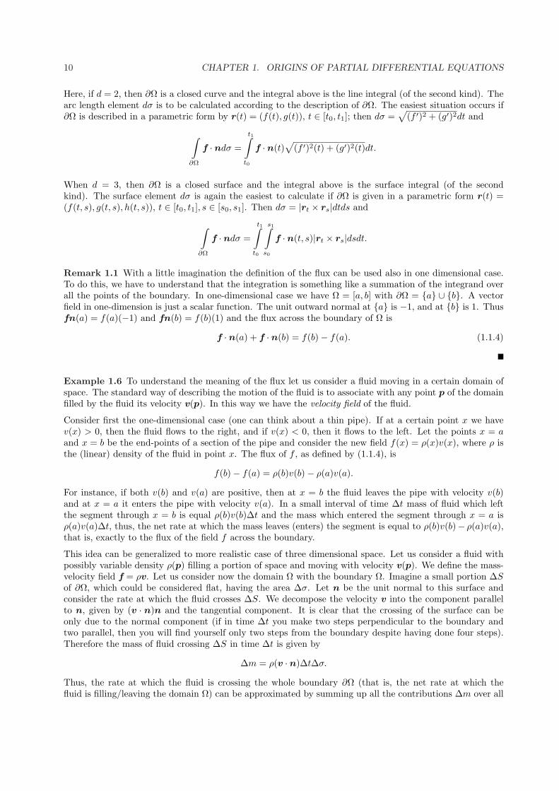
This idea can be generalized to more realistic case of three dimensional space. Let us consider a fluid withpossibly variable density ρ(p) filling a portion of space and moving with velocity v(p). We define the mass-velocity field f = ρv. Let us consider now the domain Ω with the boundary Ω. Imagine a small portion ∆Sof ∂Ω, which could be considered flat, having the area ∆σ. Let n be the unit normal to this surface andconsider the rate at which the fluid crosses ∆S. We decompose the velocity v into the component parallelto n, given by (v · n)n and the tangential component. It is clear that the crossing of the surface can beonly due to the normal component (if in time ∆t you make two steps perpendicular to the boundary andtwo parallel, then you will find yourself only two steps from the boundary despite having done four steps).Therefore the mass of fluid crossing ∆S in time ∆t is given by
∆m = ρ(v · n)∆t∆σ.
Thus, the rate at which the fluid is crossing the whole boundary ∂Ω (that is, the net rate at which thefluid is filling/leaving the domain Ω) can be approximated by summing up all the contributions ∆m over all
1. BASIC FACTS FROM CALCULUS 11
Fig. 3.2 The fluid that flows through the patch ∆S in a short time ∆t fills a slanted cylinder whose volumeis approximately equal to the base times height - v · n∆σ∆t. The mass of the fluid in the cylinder is then
ρ(v · n)Deltaσ∆t.
patches ∆S of the boundary which, in the limit as ∆S go to zero, is nothing but the flux of f:
∫
∂Ω
(ρv · n)dσ.
Thus again we have the identity
Flux of ρv across ∂Ω = the net rate at which the mass of fluid is leaving Ω.
Let us return now to the Green-Gauss-.... Theorem. This is a theorem which relates the behaviour of avector field on the boundary of a domain (flux) with what is happening inside the domain.
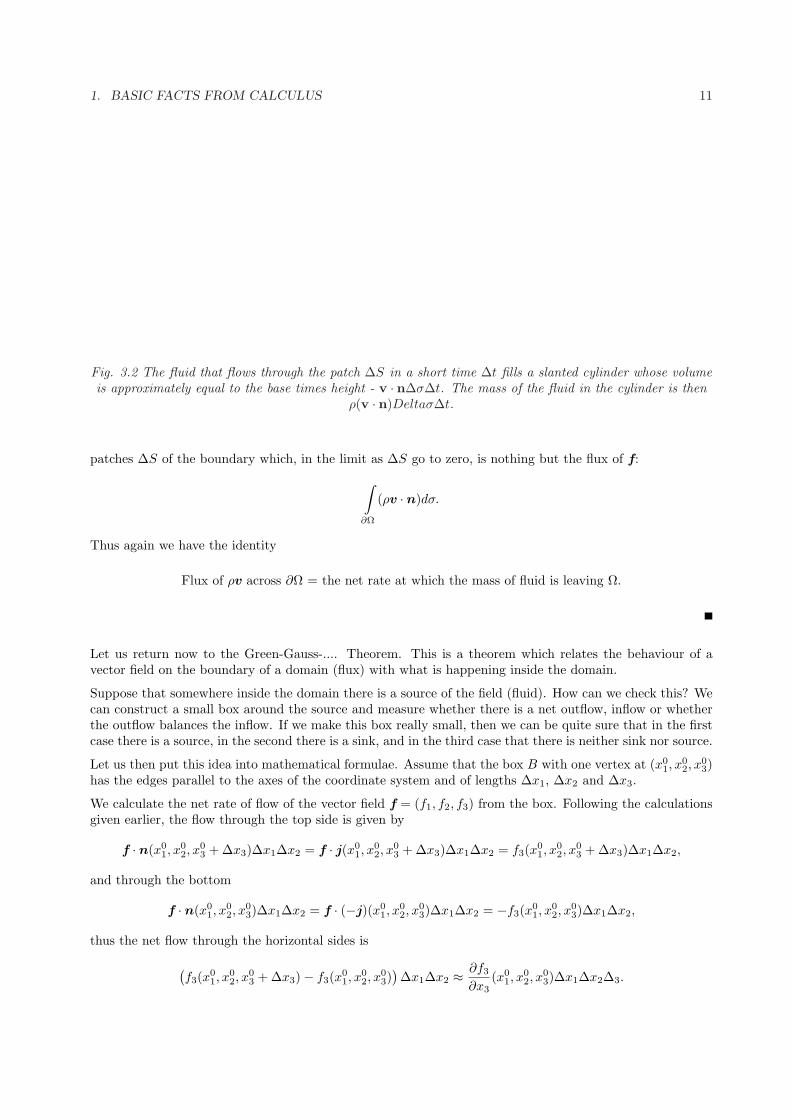
Suppose that somewhere inside the domain there is a source of the field (fluid). How can we check this? Wecan construct a small box around the source and measure whether there is a net outflow, inflow or whetherthe outflow balances the inflow. If we make this box really small, then we can be quite sure that in the firstcase there is a source, in the second there is a sink, and in the third case that there is neither sink nor source.
Let us then put this idea into mathematical formulae. Assume that the box B with one vertex at (x01, x
02, x
03)
has the edges parallel to the axes of the coordinate system and of lengths ∆x1, ∆x2 and ∆x3.
We calculate the net rate of flow of the vector field f = (f1, f2, f3) from the box. Following the calculationsgiven earlier, the flow through the top side is given by
f · n(x01, x
02, x
03 + ∆x3)∆x1∆x2 = f · j(x0
1, x02, x
03 + ∆x3)∆x1∆x2 = f3(x0
1, x02, x
03 + ∆x3)∆x1∆x2,
and through the bottom
f · n(x01, x
02, x
03)∆x1∆x2 = f · (−j)(x0
1, x02, x
03)∆x1∆x2 = −f3(x0
1, x02, x
03)∆x1∆x2,
thus the net flow through the horizontal sides is
(f3(x0
1, x02, x
03 + ∆x3)− f3(x0
1, x02, x
03)
)∆x1∆x2 ≈ ∂f3
∂x3(x0
1, x02, x
03)∆x1∆x2∆3.
12 CHAPTER 1. ORIGINS OF PARTIAL DIFFERENTIAL EQUATIONS
Similar calculations can be done for the two remaining pairs of the sides and the total flow from the box canbe approximated by (
3∑i=1
∂fi
∂xi(x0
1, x02, x
03))
)∆x1∆x2∆3.
This expression can be considered to be the net rate of the production of the field (fluid) in the box B. Theexpression
div f =3∑
i=1
∂fi
∂xi
is called the divergence of the vector field f and can considered to be the rate of the production per unitvolume (density). To obtain the total net rate of the production in the domain Ω we have to add upcontributions coming from all the (small) boxes. Thus using the definition of the integral we obtain that thetotal net rate of the production is given by
∫∫
Ω
∫div f(x1, x2, x3)dv.
Using some common sense reasoning it is easy to arrive at the identity
The net rate of production in Ω = The net flow across the boundary
The Green–Gauss–... Theorem is the mathematical expression of the above law.
Theorem 1.3 Let Ω be a bounded domain in Rd, d ≥ 1, with a piecewise C1 boundary ∂Ω. Let n be theunit outward normal vector on ∂Ω. Let f(x) = (f1(x), · · · , fn(x)) be any C1 vector field on Ω = Ω ∪ ∂Ω.Then ∫
Ω
div fdx =∮
∂Ω
f · ndσ, (1.1.5)
where dσ is the element of surface of ∂Ω.
Remark 1.2 In one dimension this theorem is nothing but the fundamental theorem of calculus:
b∫
a
df
dx(x)dx = f(b)− f(a). (1.1.6)
In fact, for a function of one variable divf = dfdx and the right-hand side of this equation represents the
outward flux across the boundary of Ω = [a, b], as discussed in Remark 1.1.
Remark 1.3 In two dimensions the most popular form of this theorem is known as the Green Theoremwhich apparently differs form the one given above. To explain this, let the boundary ∂Ω of Ω be a curvegiven by parametric equation r(t) = (x1(t), x2(t)), t ∈ [t0, t1] and suppose that if t runs from t0 to t1, thenr(t) traces ∂Ω in the positive (anticlockwise) direction. Then it is easy to check that the unit outward normalvector n is given by
n(t) =1
r′(t)(x′2(t),−x′1(t)),
where r′(t) = (x1(t), x2(t)). Thus, if f = (f1, f2), then Eq. (1.1.5) takes the form
∫∫
Ω
(∂f1
∂x1+
∂f2
∂x2
)dx1dx2 =
t1∫
t0
(f1(t)x′2(t)− f1(t)x′1(t)) dt (1.1.7)
2. CONSERVATION LAWS 13
On the other hand, the standard version of Green’s theorem reads
∫∫
Ω
(∂f2
∂x1− ∂f1
∂x2
)dx1dx2 =
∮
∂Ω
f1dx1 + f2dx2 =
t1∫
t0
(f1(t)x′1(t) + f2(t)x′2(t)) dt. (1.1.8)
To see that these forms are really equivalent, let us define the new vector field g = (g1, g2) by : g1 = −f2, g2 =f1. Then
div f =∂f1
∂x1+
∂f2
∂x2=
∂g2
∂x1− ∂g1
∂x2.
The boundary of ∂Ω is, as above, parameterized by the function r(t). Thus, if we assume that (1.1.8) holds(for an arbitrary vector field), then
∫∫
Ω
(∂f1
∂x1+
∂f2
∂x2
)dx1dx2 =
∫∫
Ω
(∂g2
∂x1− ∂g1
∂x2
)dx1dx2
=
t1∫
t0
(g1(t)x′1(t) + g2(t)x′2(t)) dt =
t1∫
t0
(f1(t)x′2(t)− f2(t)x′1(t)) dt,
which is (1.1.7). The converse is analogous.
2 Conservation laws
Many of the fundamental equations that occurr in the natural and physical sciences are obtained fromconservation laws. Conservation laws express the fact that some quantity is balanced throughout the process.
In thermodynamics, for example, the First Law of Thermodynamics states that the change in the internalenergy in a given system is equal to, or is balanced by, the total heat added to the system plus the work doneon the system. Therefore the First Law of Thermodynamics is really an energy balance, or conservation,law.
As an another example, consider a fluid flowing in some region of space that consists of chemical speciesundergoing chemical reaction. For a given chemical species, the rate of change in time of the total amountof that species in the region must equal the rate at which the species flows into the region, minus the rateat which the species flows out, plus the rate at which the species is created or consumed, by the chemicalreactions. This is a verbal statement of a conservation law for the amount of the given chemical species.
Similar balance or conservation laws occur in all branches of science. We can recall the population equationthe derivation of which was based on the observation that the rate of change of a population in a certainregion must equal the birth rate, minus the death rate, plus the migration rate into or out of the region.
Such conservation laws in mathematics are translated usually into differential equations and it is surprisinghow many different processes of real world end up with the same mathematical formulation. These differentialequations are called the governing equations of the process and dictate how the process evolves in time. Herewe discuss the derivation of some governing equations starting from the first principles. We begin with abasic one-dimensional model.
2.1 One-dimensional conservation law
Let us consider a quantity u = u(x, t) that depends on a single spatial variable x in an interval R ⊂ R,and time t > 0. We assume that u is a density, or concentration, measured in an amount per unit volume,where the amount may refer to the population, mass, energy or any other quantity. The fact that u dependsonly on one spatial variable x can be physically justified by assuming e.g. that we consider a flow in a tube,

14 CHAPTER 1. ORIGINS OF PARTIAL DIFFERENTIAL EQUATIONS
Fig. 3.3 Tube I.
which is uniform (doesn’t change in radial direction), or that the tube is very thin so that any change in theradial direction is negligible (later we shall derive the equation for the same conservation law in an arbitrarydimensional space). Note that the discussion here is related to Remark 1.1 and Example 1.6. We considerthe subinterval I = [x, x + h] ⊂ R. The total amount of the quantity u contained at time t in the section Iof the tube between x and x + h is given by the integral
total amount of quantity in I = A
x+h∫
x
u(s, t)ds,
where A is the area of the cross section of I.
Assume now that there is motion of the quantity in the tube in the axial direction. We define the flux densityof u at time t at x to be the scalar function φ(x, t) which is equal to the amount of the quantity u passingthrough the cross section at x at time t, per unit area, per unit time. By convention, the flux density at xis positive if the flow at x is in the positive x direction. Therefore, at time t the net rate that the quantityis flowing into the section is the rate that it is flowing in at x and minus the rate that it is flowing out atx + h, that is
2. CONSERVATION LAWS 15
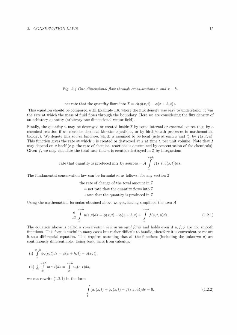
Fig. 3.4 One dimensional flow through cross-sections x and x + h.
net rate that the quantity flows into I = A(φ(x, t)− φ(x + h, t)).
This equation should be compared with Example 1.6, where the flux density was easy to understand: it wasthe rate at which the mass of fluid flows through the boundary. Here we are considering the flux density ofan arbitrary quantity (arbitrary one-dimensional vector field).
Finally, the quantity u may be destroyed or created inside I by some internal or external source (e.g. by achemical reaction if we consider chemical kinetics equations, or by birth/death processes in mathematicalbiology). We denote this source function, which is assumed to be local (acts at each x and t), by f(x, t, u).This function gives the rate at which u is created or destroyed at x at time t, per unit volume. Note that fmay depend on u itself (e.g. the rate of chemical reactions is determined by concentration of the chemicals).Given f , we may calculate the total rate that u is created/destroyed in I by integration:
rate that quantity is produced in I by sources = A
x+h∫
x
f(s, t, u(s, t))ds.
The fundamental conservation law can be formulated as follows: for any section Ithe rate of change of the total amount in I
= net rate that the quantity flows into I+rate that the quantity is produced in I
Using the mathematical formulas obtained above we get, having simplified the area A
d
dt
x+h∫
x
u(s, t)ds = φ(x, t)− φ(x + h, t) +
x+h∫
x
f(s, t, u)ds. (1.2.1)
The equation above is called a conservation law in integral form and holds even if u, f, φ are not smoothfunctions. This form is useful in many cases but rather difficult to handle, therefore it is convenient to reduceit to a differential equation. This requires assuming that all the functions (including the unknown u) arecontinuously differentiable. Using basic facts from calculus:
(i)x+h∫x
φs(s, t)ds = φ(x + h, t)− φ(x, t),
(ii) ddt
x+h∫x
u(s, t)ds =x+h∫x
ut(s, t)ds,
we can rewrite (1.2.1) in the form∫
I
(ut(s, t) + φs(s, t)− f(s, t, u))ds = 0. (1.2.2)
16 CHAPTER 1. ORIGINS OF PARTIAL DIFFERENTIAL EQUATIONS
Since this equation is valid for any interval I we can use Theorem 1.2 to infer that the integral must vanishidentically; that is, changing the independent variable back into x we must have
ut(x, t) + φx(x, t) = f(x, t, u) (1.2.3)
for any x ∈ R and t > 0. Note that in (1.2.3) we have two unknown functions: u and φ; function f is assumedto be given. Function φ is usually to be determined from empirical considerations. Equations resulting fromsuch considerations, which specify φ, are often called constitutive relations or equations of state.
Before we proceed in this direction, we shall show how the procedure described above works in higherdimensions.
2.2 Conservation laws in higher dimensions
It is relatively straightforward to generalize the discussion above to multidimensional space. Let x =(x1, x2, x3) denote a point in R3 and assume that u = u(x, t) is a scalar density function representingthe amount per unit volume of some quantity of interest distributed throughout some domain of R3. In thisdomain, let Ω ⊂ R3 be an arbitrary region with a smooth boundary ∂Ω. As in one-dimensional case, thetotal amount of the quantity in Ω at time t is given by the integral
∫
Ω
u(x, t)dx,
and the rate that the quantity is produced in Ω is given by∫
Ω
f(x, t, u)dx,
where f is the rate at which the quantity is being produced in Ω.
Some changes are required however when we want to calculate the flux of the quantity in or out Ω. Becausenow the flow can occur in any direction, the flux density is given by a vector Φ (in Example 1.6, it wasgiven by ρ(x)v(x)). However, as we noted in this example, not all the flowing quantity which is close to theboundary will leave or enter the region Ω – the component of Φ which is tangential to the boundary ∂Ω willnot contribute to the total loss (see also Fig. 2.1). Therefore, if we denote by n(x) the outward unit normalvector to ∂Ω, then the net outward flux of the quantity u through the boundary ∂Ω is given by the surfaceintegral ∫
∂Ω
Φ(x, t) · n(x)dσ,
where dσ denotes a surface element on ∂Ω. Finally, the balance law for u is given by
d
dt
∫
∂Ω
udx = −∮
∂Ω
Φ · ndσ +∫
Ω
fdx. (1.2.4)
The minus sign at the flux term occurs because the outward flux decreases the amount of u in Ω.
As before, the integral form can be reformulated as a local differential equation, provided Φ and u aresufficiently smooth in x and t. To this end we must use the Gauss theorem (Theorem 1.3) which gives
∫
∂Ω
Φ · ndσ =∫
Ω
div Φdx.
Using this formula, Equation (1.2.4) can be rewritten as∫
Ω
(ut + div Φ− f) dx = 0
3. CONSTITUTIVE RELATIONS AND EXAMPLES 17
for any subregion Ω. Using the vanishing theorem (Theorem 1.2) we finally obtain the differential form ofthe general conservation law in 3 (or higher) dimensional space
ut + div Φ = f(x, t, u). (1.2.5)
In the next section we discuss a number of constitutive relations which provide examples of the flux function.
3 Constitutive relations and examples
In this section we describe a few constitutive relation which often appear in the applied sciences. It isimportant to understand that a constitutive relations appear on a different level than conservation law: thelatter is is a fundamental law of nature – the mathematical expression of the fact that books should balance(at least in a decent(?) enterprise like the Universe), whereas the former is often an approximate equationhaving its origins in empirics.
3.1 Transport equation
Probably the simplest nontrivial constitutive relation is when the quantity of interest moves together withthe surrounding medium with a given velocity, say, v. This can be a simple model for a low density pollutantin the air moving only due to wind with velocity v or, as we discussed earlier, fluid with density u movingwith the velocity v. Then the flux density is given by
Φ = vu
and, if there are no sources or sinks, the transport equation is given by
ut + div (vu) = 0. (1.3.1)
We can rewrite this equation in a more explicit form
ut + v · ∇u + udiv v = 0,
or, if the velocity is constant or, more general, divergence (or source) free,
∂tu + v · ∇u = 0. (1.3.2)
In more general cases, v may depend on the solution u itself. For example, (1.3.1) may describe a motionof a herd of animals over certain area with u being (suitably rounded) density of animals per, say, squarekilometer. Then the speed of the herd will depend on the density - the bigger the squeeze, the slower theanimals move. This constitutes an example of a quasilinear equation in which the coefficient of the highestderivative depend on the solution:
ut + div (v(u)u) = 0. (1.3.3)
3.2 McKendrick partial differential equation
The derivation of the conservation law was based on a physical intuition about a fluid flow in a physicalspace. Yet the argument can be used in a much broader context. Consider an age-structured population,described by the density of the population n(a, t) with respect to age n(a, t), and look at the population asif it was ’transported’ through stages of life. Taking into account that n(a, t)∆a is the number of individuals(females) in the age group [a, a + ∆a) at time t, we may write that the rate of change of this number
∂
∂t[n(a, t)∆a]
18 CHAPTER 1. ORIGINS OF PARTIAL DIFFERENTIAL EQUATIONS
equals rate of entry at a minus rate of exit at a + ∆a and minus deaths. Denoting per capita mortality ratefor individuals by µ(a, t), the last term is simply −µ(a, t)n(a, t)∆t. The first two terms require introductionof the ’flux density’ of individuals J describing the ‘speed’ of ageing. Thus, passing to the limit ∆a → 0, weget
∂n(a, t)∂t
+∂J(a, t)
∂a= −µ(a, t)n(a, t).
Let us determine the flux density in the simplest case when ageing is just the passage of time measured inthe same units.
Here for consistency, we derive the full equation. If the number of individuals in the age bracket [a, a + ∆a)is n(a, t)∆a, then after ∆t we will have n(a, t+∆t)∆a. On the other hand, u(a−∆t, t)∆t individuals movedin while u(a + ∆a−∆t, t)∆t moved out, where we assumed, for simplicity, ∆t < ∆a. Thus
n(a, t + ∆t)∆a− n(a, t)∆a = u(a−∆t, t)∆t− u(a + ∆a−∆t)∆t− µ(a, t)n(a, t)∆a∆t
or, using the Mean Value Theorem (0 ≤ θ, θ′ ≤ 1)
nt(a, t + θ∆t)∆a∆t = −na(a−∆t + θ′∆a, t)∆a∆t− µ(a, t)n(a, t)∆a∆t
and, passing to the limit with ∆t,∆a → 0, we obtain
∂n(a, t)∂t
+∂n(a, t)
∂a= −µ(a, t)n(a, t). (1.3.4)
This equation is defined for a > 0 and the flow is to the right hence we need a boundary condition. In thismodel the birth rate enters here: the number of neonates (a = 0) is the number of births across the wholeage range:
n(0, t) =
ω∫
0
n(a, t)m(a, t)da,
where m is the maternity function. Eq. (1.3.4) also must be supplemented by the initial condition
n(a, 0) = n0(a)
describing the initial age distribution.
3.3 Diffusion/heat equations
Assume at first that there are no sources, and write the basic conservation law in one-dimension as
ut + φx = 0 (1.3.5)
In many physical (and not only) problems it was observed that the substance (represented here by the densityu) moves from the regions of higher concentration to regions of lower concentration (heat, population, etc.offer a good illustration of this). Moreover, the larger difference the more rapid flow is observed. At a point,the large difference can be expressed as a large gradient of the concentration u, so it is reasonable to assumethat
φ(x, t) = −F (ux(x, t)),
where F is an increasing function passing through (0, 0). The explanation of the minus sign comes from thefact that if the x-derivative of u at x is positive, that is, u is increasing, then the flow occurs in the negativedirection of the x axis. Moreover, the larger the gradient, the larger (in magnitude) the flow. Now, thesimplest increasing function passing through (0, 0) is a linear function with positive leading coefficient, andthis assumption gives the so-called Fick law:
φ(x, t) = −Dux(x, t) (1.3.6)
3. CONSTITUTIVE RELATIONS AND EXAMPLES 19
where D is a constant which is to be determined empirically. We can substitute Fick’s law (1.3.6) into theconservation law (1.2.3) (assuming that the solution is twice differentiable and D is a constant) and get theone dimensional diffusion equation
ut −Duxx = 0, (1.3.7)
which governs conservative processes when the flux is specified by Fick’s law.
To understand why this equation governs also the evolution of the temperature distribution in a body, weapply the conservation law (1.2.3) to heat (thermal energy). Then the amount of heat in a unit volumecan be written as u = cρθ, where c is the specific heat of the medium, ρ the density of the medium andθ is the temperature. The heat flow is governed by Fourier’s law which states that the heat flux densityis proportional to the gradient of the temperature, with the proportionality constant equal to −k, wherek is the thermal conductivity of the medium. Assuming c, ρ, k to be constants, we arrive at (1.3.7) withD = k/cρ.
Generalization of Equation (1.3.7) to multidimensional cases requires some assumptions on the medium. Tosimplify the discussion we assume that the medium is isotropic, that is, the process of diffusion is independentof the orientation in space. Then the Fick law states that the flux density is proportional to the gradient ofu, that is,
Φ = −D∇u
and the diffusion equation, obtained from the conservation law (1.2.5) in the absence of sources, reads
ut = div(D∇u) = D∆u, (1.3.8)
where the second equality is valid if D is a constant.
3.4 Variations of diffusion equation
In many cases the evolution is governed by more then one process. One of the most widely occuring cases iswhen we have simultaneously both transport and diffusion. For example, when we have a pollutant in theair or water, then it is transported with the moving medium (due to the wind or water flow) and, at thesame time, it is dispersed by diffusion. Without the latter, a cloud of pollution would travel without anychange - the same amount that was released from the factory would eventually reach other places with thesame concentration. Diffusion, as we shall see later, has a dispersing effect, that is, the pollution will beeventually deposited but in a uniform, less concentrated way, making life (perhaps) more bearable.
Mathematical expression of the above consideration is obtained by combining equations (1.3.1) and (1.3.8):
ut + div (vu) = D∆u, (1.3.9)
or, equivalently, by determining the expression for the flux taking both processes simultaneously into account.The resulting equation (1.3.9) is called the drift-diffusion equation.
When the sources are present and the constitutive relation is given by Fick’s law, then the resulting equation
ut −D∆u = f(x, t, u) (1.3.10)
is called the reaction-diffusion equation. If f is independent of u, then physically we have the situationwhen the sources are given a priori (like the injection performed by an observer); the equation becomes thena linear non-homogeneous equation. Sources, however, can depend on u. The simplest case is then whenf = cu with c constant. Then the source term describes spontaneous decay (or creation) of the substance atthe rate that is proportional to the concentration. In such a case Equation (1.3.10) takes the form
ut −D∆u = cu (1.3.11)
and can be thought of as the combination of the diffusion and the law of exponential growth.

20 CHAPTER 1. ORIGINS OF PARTIAL DIFFERENTIAL EQUATIONS
If f is nonlinear in u, then Equation (1.3.10) has many important applications, particularly in the combustiontheory and mathematical biology.
Here we describe the so called Fisher equation which appears as a combination of the one-dimensional logisticprocess and the diffusion. It is reasonable to assume that the population is governed by the logistic law,which is mathematically expressed as the ordinary differential equation
du
dt= ru(N − u), (1.3.12)
where u is the population in some region, rN > 0 is the growth rate and N > 0 is the carrying capacity ofthis region. If we are however interested is the spatial distribution of individuals, then we must introducethe density of the population u(x, t), that is, the amount of individuals per unit of volume (or surface) andthe conservation law will take the form
ut + div Φ = ru (N − u) . (1.3.13)
As a first approximation, it is reasonable to assume that within the region the population obeys the Ficklaw, that is, individuals migrate from the regions of higher density to regions of lower density. This isnot always true (think about people migrating to cities) and therefore the range of validity of Fick’s lawis limited; in such cases Φ has to be determined otherwise. However, if we assume that the resources areevenly distributed, then Fick’s law can be used with good accuracy. In such a case, Equation (1.3.13) takesthe form
ut −D∆u = ru (N − u) , (1.3.14)
which is called the Fisher equation. Note, that if the capacity of the region N is very large, then writing theFisher equation in the form
ut −D∆u = cu(1− u
N
),
where c = rN , we see that it is reasonable to neglect the small term u/N and approximate the Fisherequation by the linear equation (5.5.15) which describes a combination of diffusion-type migratory processesand exponential growth.
Chapter 2
First order linear partial differentialequations
1 Basic theory and examples
We start with the simplest transport equation. Assume that u is a concentration of some substance (pollu-tant) in a fluid (amount per unit length). This substance is moving to the right with a speed c. Then thedifferential equation for u has the form:
ut + cux = 0. (2.1.1)
Let us consider more general linear first order partial differential equation (PDE) of the form:
aut + bux = 0, t, x ∈ R (2.1.2)
where a and b are constants. This equation can be written as
Dvu = 0, (2.1.3)
where v = aj+ bi (j and i are the unit vectors in, respectively, t and x directions), and Dv = ∇u ·v denotesthe directional derivative in the direction of v. This means that the solution u is a constant function alongeach line having direction v, that is, along each line of equation bt−ax = ξ. Along each such a line the valueof the parameter ξ remains constant. However, the solution can change from one line to another, thereforethe solution is a function of ξ, that is the solution to Eq. (2.1.2) is given by
u(x, t) = f(bt− ax), (2.1.4)
where f is an arbitrary differentiable function. Such lines are called the characteristic lines of the equation.
Example 1.1 To obtain a unique solution we must specify the initial value for u. Hence, let us considerthe initial value problem for Eq. (2.1.2): find u satisfying both
aut + bux = 0 x ∈ R, t > 0,
u(x, 0) = g(x) x ∈ R, (2.1.5)
where g is an arbitrary given function. From Eq. (2.1.4) we find that
u(x, t) = g
(−bt− ax
a
). (2.1.6)
We note that the initial shape propagates without any change along the characteristic lines, as seen belowfor the initial function g = 1− x2 for |x| < 1 and zero elsewhere. The speed c = b/a is taken to be equal to1.
21

22 CHAPTER 2. FIRST ORDER LINEAR PARTIAL DIFFERENTIAL EQUATIONS
Fig. 4.1 The graph of the solution in Example 1.1
Example 1.2 Let us consider a variation of this problem and try to solve the initial- boundary value problem
aut + bux = 0 x ∈ R, t > 0,
u(x, 0) = g(x) x > 0, (2.1.7)u(0, t) = h(t) t > 0, (2.1.8)
for a, b > 0 From Example 1.1 we have the general solution of the equation in the form
u(x, t) = f(bt− ax).
Putting t = 0 we get f(−ax) = g(x) for x > 0, hence f(x) = g(−x/a) for x < 0. Next, for x = 0 we obtainf(bt) = h(t) for t > 0, hence f(x) = h(x/b) for x > 0. Combining these two equations we obtain
u(x, t) =
g(− bt−axa ) for x > bt/a
h( bt−axb ) for x < bt/a
Now, let us consider what happens if a = 1 > 0, b = −1 < 0. Then the initial condition defines f(x) = g(−x)for x < 0 and the boundary condition gives f(x) = h(−x) also for x < 0! Hence, we cannot specify bothinitial and boundary conditions in an arbitrary way as this could make the problem ill-posed.
The physical explanation of this comes from the observation that since the characteristics are given byξ = x + t, the flow occurs in the negative direction and therefore the values at x = 0 for any t are uniquelydetermined by the initial condition. Therefore we see that to have a well-posed problem we must specify theboundary conditions at the point where the medium flows into the region.
The same principle could be used to solve equations with variable coefficients. In fact, consider the equation
a(x, t)ut + b(x, t)ux = f(x, t, u). (2.1.9)
This equation asserts that the derivative of u in the direction of the vector (b(x, t), a(t, x)) is equal to f(x, t, u)at each point (x, t) where this vector is not vanishing. We can consider a family of curves τ → (x(τ), t(τ))which are tangent to these vectors at each point. In other words, we consider the family of curves determinedby the system of differential equations
xτ = b(x, t), tτ = a(x, t) (2.1.10)
subject to the initial condition x(0) = ξ, and t(0) = 0, expressing the fact that the curves cross the line t = 0at τ = 0 at an unspecified for a time being point x = ξ. Let Iξ be an interval of existence of the solution
1. BASIC THEORY AND EXAMPLES 23
passing through ξ. The curves (x(τ, ξ), t(τ, ξ))τ∈Iξare called the characteristics of the system. We note that,
depending on the properties of the vector field (b, a), the system (2.1.10) may not have a solution, may havenon-unique solutions, the solutions may exist for a finite time interval and also may fill only a region of R2.
Let us consider a characteristic τ → (x(τ, ξ), t(τ)) lying in the domain D of the (x, t)-plane in which thereis a differentiable solution u of (2.1.9). Then we can define
v(ξ, τ) = u(x(τ, ξ), t(τ, ξ))
and, differentiating with respect to τ we find, by the chain rule,
vτ = uttτ + uxxτ = uta + uxb = g
where g(τ, ξ) := f(x(τ, ξ), t(τ, ξ), v(ξ, τ)). Thus, the partial differential equation (2.1.9) reduces to a firstorder ordinary equation which requires an initial condition. Since we have u(x, 0) = u0(x), for v we canwrite
v(ξ, 0) = u(x(0, ξ), t(0, ξ)) = u(ξ, 0) = u0(ξ).
Conversely, if u is a differentiable function of two variables such that v(τ, ξ) = u(x(τ, ξ), t(τ, ξ)) satisfies thesystem
vτ = g,
xτ = b,
tτ = a,
v(0) = u0(ξ), x(0) = ξ, t(0) = 0, (2.1.11)
then u(x, t) solves (2.1.9) at any point (x, t) through which a characteristic passes.
This indicates a way to solving
a(x, t)ut(x, t) + b(x, t)ux(x, y) = f(x, t, u(x, t)), u(x, 0) = u0(x), x ∈ R, t ≥ 0. (2.1.12)
DefineE = (x, t); x = x(τ, ξ), t = t(τ, ξ), ξ ∈ R, τ ∈ Iξ,
so that E is a set filled with characteristics starting from t = 0. If the field (b, a) is Lipschitz continuous,then these characteristics do not cross each other and thus present a new coordinate system. Then, for any(x, t) ∈ E there is a unique characteristic passing through (x, t); that is, there is unique pair (ξ, τ) such thatx = x(ξ, τ), t = t(ξ, τ) and then
u(x, t) = v(ξ(x, t), τ(x, t))
is the solution of (2.1.12).
The above considerations can be simplified if a 6= 0. Then dividing the equation by a we arrive at anequivalent form
ut + c(x, t)ux = f(x, t, u),u(x, 0) = u0(x). (2.1.13)
In this case we have tτ = 1 and thus we can take t = τ reducing the number of equations by 1. Then thesystem (2.1.11)
vt(ξ, t) = g(ξ, t, v(ξ, t)) = f(x(t, ξ), t, v(ξ, t)),xt = c(x, t),
x(0) = ξ, v(0, ξ) = u0(ξ), (2.1.14)
which, in principle, can be solved. The second equation is independent of the first so that it determines theequation of characteristics x = x(t, ξ). This solution can be substituted into the first equation the solutionof which gives the values of v as a function of t that is a parameter along a characteristic. Eliminating ξfrom equations for v and x produces the solution u in terms of x and t only.
We illustrate the method in the examples below.
24 CHAPTER 2. FIRST ORDER LINEAR PARTIAL DIFFERENTIAL EQUATIONS
Example 1.3 Find the solution of the equation
ut + 2ux = x, x ∈ R,
which satisfies the initial condition:u(x, 0) = v0(x).
The characteristic equation isxt = 2, x(0) = ξ
giving the characteristicsx− 2t = ξ
Then v(t, ξ) = u(x(t, ξ), t), x = 2t + ξ and
vt = 2t + ξ, v(ξ, 0) = v0(ξ),
so that we havev(t, ξ) = c + t2 + ξt.
To determine c we put t = 0 so thatv(0, ξ) = c = v0(ξ).
Thusv(t, ξ) = t2 + ξt + v0(ξ).
To find the solution u(x, t) we must revert to old variables. Using again the characteristic equation, we havex− 2t = ξ so that
u(x, t) = v(t, x− 2t) = t2 + (x− 2t)t + v0(x− 2t) = xt− t2 + v0(x− 2t).
In the next example we consider an initial-boundary value problem. In many one-dimensional cases weencounter the so called signalling problem when the boundary condition is prescribed at one end-point of ahalf-line.
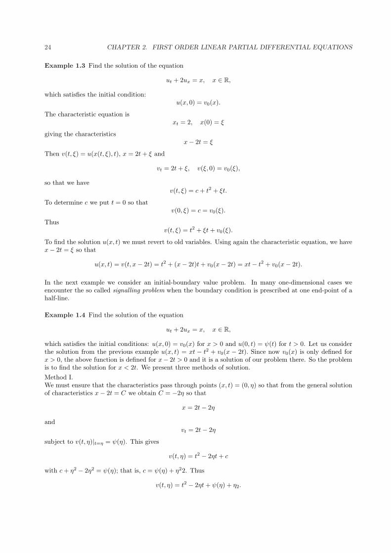
Example 1.4 Find the solution of the equation
ut + 2ux = x, x ∈ R,
which satisfies the initial conditions: u(x, 0) = v0(x) for x > 0 and u(0, t) = ψ(t) for t > 0. Let us considerthe solution from the previous example u(x, t) = xt − t2 + v0(x − 2t). Since now v0(x) is only defined forx > 0, the above function is defined for x− 2t > 0 and it is a solution of our problem there. So the problemis to find the solution for x < 2t. We present three methods of solution.Method I.We must ensure that the characteristics pass through points (x, t) = (0, η) so that from the general solutionof characteristics x− 2t = C we obtain C = −2η so that
x = 2t− 2η
andvt = 2t− 2η
subject to v(t, η)|t=η = ψ(η). This gives
v(t, η) = t2 − 2ηt + c
with c + η2 − 2η2 = ψ(η); that is, c = ψ(η) + η22. Thus
v(t, η) = t2 − 2ηt + ψ(η) + η2.
1. BASIC THEORY AND EXAMPLES 25
Returning to the original variables, we find that for x < 2t
u(x, t) = v(t, t− x/2) = t2 − 2t(t− x/2) + (t− x/2)2 + ψ(t− x/2) = ψ(t− x/2) + x2/4.
Method 2.We observe that for the boundary value part, the variables interchange their roles. Thus, we can re-writethe equation as
ux +12ut =
x
2and proceed as before. Thus, the characteristic equation becomes
tx =12
with the initial condition t(0) = η giving t− x/2 = η. However, contrary to the previous method, now x isthe independent variable so that u(x, t) = u(t, t(x)) = v(x, η) and we obtain
vx =x
2, v(0) = ψ(η)
yielding
v(x, η) =14x2 + g(η)
or, in the old variables,
u(x, t) =14x2 + ψ(t− x/2), x > 2t,
exactly as in the previous method.
Method 3.In this method we pretend that we know the initial condition on the whole line and will try to match thissolution to the particular boundary condition. Thus, consider the solution
u(x, t) = xt− t2 + φ(x− 2t).
for some function φ. Since φ(x) = v0(x) for x > 0, the above function is a solution to our problem forx > t/2. On the other hand, we need u(0, t) = ψ(t) so that
ψ(t) = −t2 + φ(−2t)
which gives φ(s) = s2/4 + ψ(−s/2) for s < 0. Hence, for x < t/2,
u(x, t) = xt− t2 + (x− 2t)2/4 + ψ(t− x/2) = x2/4 + ψ(t− x/2)
as previously.
Example 1.5 Find the solution to the following initial value problem
ut + xux + u = 0, t > 0, x ∈ R,
u(x, 0) = u0(x),
where u0(x) = 1− x2 for |x| < 1, and u0(x) = 0 for |x| ≥ 1. The characteristic system is
vt = −v,
xt = x, (2.1.15)
with the initial conditions v(0, ξ) = u0(ξ), x(0, ξ) = ξ where ξ is the intercept of the characteristic and thex-axis. The general solution of (2.1.15) is
v(t, ξ) = ae−t, x(t, ξ) = bet,
26 CHAPTER 2. FIRST ORDER LINEAR PARTIAL DIFFERENTIAL EQUATIONS
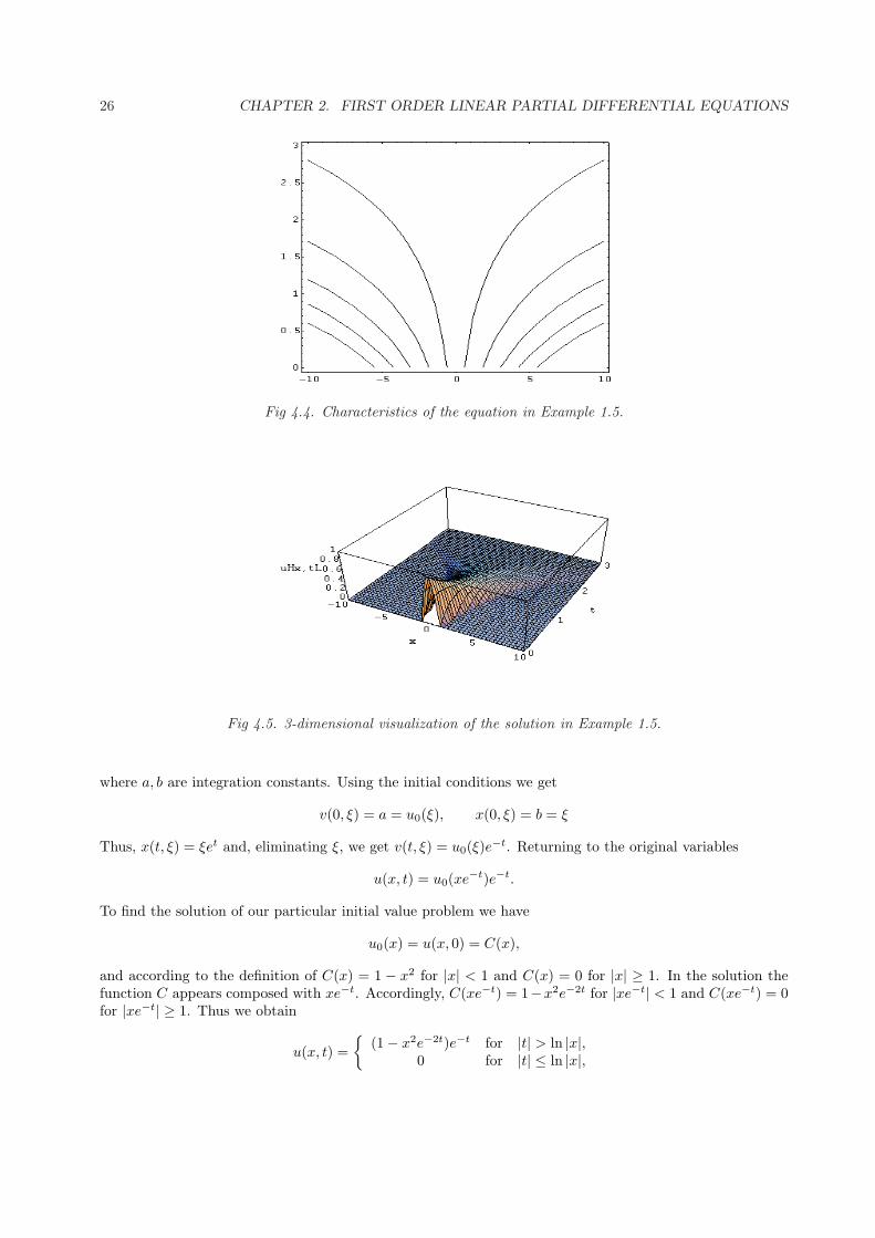
Fig 4.4. Characteristics of the equation in Example 1.5.
Fig 4.5. 3-dimensional visualization of the solution in Example 1.5.
where a, b are integration constants. Using the initial conditions we get
v(0, ξ) = a = u0(ξ), x(0, ξ) = b = ξ
Thus, x(t, ξ) = ξet and, eliminating ξ, we get v(t, ξ) = u0(ξ)e−t. Returning to the original variables
u(x, t) = u0(xe−t)e−t.
To find the solution of our particular initial value problem we have
u0(x) = u(x, 0) = C(x),
and according to the definition of C(x) = 1 − x2 for |x| < 1 and C(x) = 0 for |x| ≥ 1. In the solution thefunction C appears composed with xe−t. Accordingly, C(xe−t) = 1−x2e−2t for |xe−t| < 1 and C(xe−t) = 0for |xe−t| ≥ 1. Thus we obtain
u(x, t) =
(1− x2e−2t)e−t for |t| > ln |x|,0 for |t| ≤ ln |x|,
1. BASIC THEORY AND EXAMPLES 27
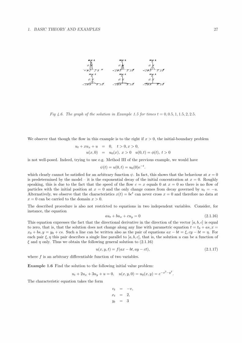
Fig 4.6. The graph of the solution in Example 1.5 for times t = 0, 0.5, 1, 1.5, 2, 2.5.
We observe that though the flow in this example is to the right if x > 0, the initial-boundary problem
ut + xux + u = 0, t > 0, x > 0,
u(x, 0) = u0(x), x > 0 u(0, t) = φ(t), t > 0
is not well-posed. Indeed, trying to use e.g. Method III of the previous example, we would have
ψ(t) = u(0, t) = u0(0)e−t.
which clearly cannot be satisfied for an arbitrary function ψ. In fact, this shows that the behaviour at x = 0is predetermined by the model – it is the exponential decay of the initial concentration at x = 0. Roughlyspeaking, this is due to the fact that the speed of the flow c = x equals 0 at x = 0 so there is no flow ofparticles with the initial position at x = 0 and the only change comes from decay governed by ut = −u.Alternatively, we observe that the characteristics x(t) = bet can never cross x = 0 and therefore no data atx = 0 can be carried to the domain x > 0.
The described procedure is also not restricted to equations in two independent variables. Consider, forinstance, the equation
aut + bux + cuy = 0 (2.1.16)
This equation expresses the fact that the directional derivative in the direction of the vector [a, b, c] is equalto zero, that is, that the solution does not change along any line with parametric equation t = t0 + as, x =x0 + bs, y = y0 + cs. Such a line can be written also as the pair of equations ax − bt = ξ, cy − bt = η. Foreach pair ξ, η this pair describes a single line parallel to [a, b, c], that is, the solution u can be a function ofξ and η only. Thus we obtain the following general solution to (2.1.16)
u(x, y, t) = f(ax− bt, ay − ct), (2.1.17)
where f is an arbitrary differentiable function of two variables.
Example 1.6 Find the solution to the following initial value problem:
ut + 2ux + 3uy + u = 0, u(x, y, 0) = u0(x, y) = e−x2−y2.
The characteristic equation takes the form
vt = −v,
xt = 2,
yt = 3
28 CHAPTER 2. FIRST ORDER LINEAR PARTIAL DIFFERENTIAL EQUATIONS
with initial conditions v(0, ξ, η) = u0(ξ, η), x(0, ξ, η) = ξ, y(0, ξ, η) = η. Then x− 2t = ξ, y − 3t = η and
v(t, ξ, η) = C(ξ, η)e−t.
Thus, C(ξ, η) = u0(ξ, η) andu(x, y, t) = u0(x− 2t, y − 3t)e−t.
Finally, using the initial equation, we get
u(x, y, t) = e−(x−2t)2−(y−3t)2e−t.
1.1 The McKendrick equation
Consider the simplified population dynamics problem
nt(a, t) + na(a, t) = −µn(a, t). (2.1.18)
coupled with the boundary condition
n(0, t) = m
∞∫
0
n(a, t)da,
and the initial conditionn(a, 0) = n0(a).
First, let us simplify the equation (2.1.18) by introducing the integrating factor
(eµan(a, t))t = −(eµan(a, t))a
and denote u(a, t) = eµan(a, t). Then
u(0, t) = n(0, t) = m
∞∫
0
e−µau(a, t)da
with u(a, 0) = eµan0(a) =: u0(a). Now, if we knew ψ(t) = u(0, t), then
u(a, t) =
u0(a− t), t < a,ψ(t− a), a < t.
(2.1.19)
The boundary condition can be rewritten as
ψ(t) = m
∞∫
0
e−µau(a, t)da = m
t∫
0
e−µaψ(t− a)da + m
∞∫
t
e−µau0(a− t)da
= me−µt
t∫
0
eµσψ(σ)dσ + me−µt
∞∫
0
e−µru0(r)dr
which, upon denoting φ(t) = ψ(t)eµt and using the original initial value, can be written as
φ(t) = m
t∫
0
φ(σ)dσ + m
∞∫
0
n0(r)dr. (2.1.20)
Now, if we differentiate both sides, we getφ′ = mφ
1. BASIC THEORY AND EXAMPLES 29
which is just a first order linear equation. Letting t = 0 in (2.1.20) we obtain the initial value for φ:
φ(0) = m∞∫0
n0(r)dr. Then
φ(t) = memt
∞∫
0
n0(r)dr
and
ψ(t) = me(m−µ)t
∞∫
0
n0(r)dr.
Then
n(a, t) = e−µau(a, t) = e−µt
n0(a− t), t < a,
mem(t−a)∞∫0
n0(r)dr, a < t.
30 CHAPTER 2. FIRST ORDER LINEAR PARTIAL DIFFERENTIAL EQUATIONS
Chapter 3
First order nonlinear equations
1 Basic theory
The linear models discussed in the previous section described propagation of signals with speed that isindependent of the solution. This is the case for e.g. acoustic signals that propagate at a constant soundspeed. However, signals with large amplitude propagate at a speed that is proportional to the local densityof the air. Thus, it is important to consider equations in which the speed of propagation depends on thevalue of the solution. The qualitative picture in such cases is completely different than for linear equations.
We shall focus on the simple nonlinear value problem:
ut + c(u)ux = 0, x ∈ R, t > 0,
u(x, 0) = u0(x), x ∈ R. (3.1.1)
Here, c is a given smooth function of u. The above equation is simply the conservation law
ut + φ(u)x = 0
after differentiation with respect to x so that c(u) = φu(u).
To analyse (3.1.1) we assume at first that a C1 solution u(x, t) to (3.1.1) exists for all t > 0. Motivated bythe linear approach we define characteristic curves by the differential equation
dx
dt= c(u(x, t)). (3.1.2)
Of course, contrary to the situation for linear equations, the right hand side of this equation is not known apriori. Thus, characteristics cannot be determined in advance. However, assuming that we know them, wecan solve (3.1.2) getting
x = x(t, η)
where η is an integration constant. Fixing η we obtain, as in the linear case, that
d
dtu(x(t, η), t) = uxxt + ut = uxc(u) + ut = 0
thus the solution is constant any characteristic and depends only on the single variable ξ. Now, we observethat along each characteristic at each point the slope is given by c(u(x(t, ξ), t)) but this depends only onξ that is fixed along each characteristic. Thus, the slope of each characteristic is constant so that eachcharacteristic is a straight line. Alternatively, we can prove it by differentiating x = x(t, ξ) twice to get
d2x
dt2=
d
dtc(u(x(t, ξ), t)) = cu(u) · (uxxt + ut) = cu(u) · (uxc(u) + ut) = 0.
31
32 CHAPTER 3. FIRST ORDER NONLINEAR EQUATIONS
Thus, from each point (x, t) we draw a straight line to an unspecified (yet) point (ξ, 0) on the x-axis so thatthe equation of this characteristic is given by
x− ξ = c(u(ξ, 0))t = c(u0(ξ))t (3.1.3)
because the slope is constant and therefore it must be equal to the value of c(u) at the initial time t = 0.Note that since c and u0 are known functions, then (3.1.3) determines ξ implicitly in terms of a given (x, t)(if it can be solved). Since the solution u is constant along characteristics, we have the implicit formula forit
u(x, t) = u(ξ, 0) = u0(ξ)
where ξ is given by (3.1.3). In some instances (3.1.3) can be solved explicitly.
Example 1.1 Find the solution to the initial value problem
ut + uux = 0, x ∈ R, t > 0,
u(x, 0) = x.
The characteristics emanating from a point (ξ, 0) on the x-axis have speed c(u0(ξ)) = u0(ξ). Using thediscussion above we see that the solution is given implicitly by
u(x, t) = c(u0(ξ)) = ξ
wherex− ξ = tξ
so that easilyξ =
x
1 + t
and the solution is given byu(x, t) =
x
1 + t.
Note that in this example the solution is defined for values of t > 0. This is not always the case and ourprior discussion based on the assumption that for any (x, t) with t > 0 we have a smooth solution can beinvalid. However, we can prove the following result
Theorem 1.1 If the functions c and u0 are C1(R) and if u0 and c are either both nondecreasing or bothnonincreasing on R, then the initial value problem (3.1.1) has a unique solution defined implicitly by theparametric equations
u(x, t) = u0(ξ),x− ξ = c(u(ξ, 0))t = c(u0(ξ))t (3.1.4)
Proof. Since we have shown that if there is a smooth solution to (3.1.1), then it must be of the form (3.1.4),all we have to do is to show that (3.1.4) is uniquely solvable and that the function u(x, t) obtained from(3.1.4) is, in fact, a solution of (3.1.1). As we already mentioned, the second equation of (3.1.4) shoulduniquely determine ξ = ξ(x, t) for any (x, t), t > 0. This is an implicit equation of the form
F (ξ, x, t) = 0
where F (ξ, x, t) = ξ + c(u0(ξ))t− x and, from the general theory, this equation is (locally) solvable aroundany point at which Fξ 6= 0. In this case,
Fξ(ξ, x, t) = 1 + c′u(u0(ξ))u′0,ξt 6= 0
1. BASIC THEORY 33
and since from the assumption, c0, u0 are either both increasing, or both decreasing, the derivatives are ofthe same sign and the second term is always positive. Thus, under the assumptions, Fξ 6= 0 everywhere and(3.1.4) is uniquely solvable for any choice of (x, t) and ξ(x, t) is differentiable. Implicit differentiation of thefirst equation of (3.1.4) gives
ut(x, t) = u′0,ξξt, ux(x, t) = u′0,ξξx
where, by implicit differentiation of the second equation in (3.1.4),
−ξt = c′(u0(ξ))u′0,ξξtt + c(u0(ξ)), 1− ξx = c′(u0(ξ))u′0,ξξxt
so that
ut(x, t) = − c(u0(ξ))u′0,ξ
1 + c′u(u0(ξ))u′0,ξt, ux(x, t) =
u′0,ξ
1 + c′u(u0(ξ))u′0,ξt,
where the denominator is always positive by the argument above. Hence,
ut + c(u)ux = 0
and we have indeed a unique solution defined everywhere for t > 0.
The general method of characteristic system, described in Remark ?? can be used also for nonlinear equations,as illustrated in the example below. The resulting system in the nonlinear case become coupled and, in manycases, rather impossible to solve.
Example 1.2 Consider the initial value problem
ut + uux = −u, x ∈ R, t > 0
u(x, 0) = −x
2, x ∈ R.
The characteristic system for v(t, ξ) = u(x(t), t) is
dv
dt= −v,
dx
dt= v,
with the initial data v(0) = −ξ/2, x(0) = ξ. The general solution of the system is
v(t) = ae−t, x(t) = b− ae−t.
Using the initial conditions, we obtain
a = −ξ
2, b =
ξ
2,
so that
v = −ξ
2e−t, x =
ξ
2(1 + e−t
).
Dividing v by x, we eliminate ξ, getting
u(x, t) = − xe−t
1 + e−t.
This is a smooth solution defined for all x ∈ R and t > 0.
It should be stressed that the situation described in the previous two examples are far from being typical.Firstly, in most cases the implicit equation for ξ in (3.1.4) cannot be solved explicitly. Secondly, a solutionmay cease to exist after finite time, as shown in the example below.

34 CHAPTER 3. FIRST ORDER NONLINEAR EQUATIONS
Example 1.3 Consider the equation
ut + uux = 0, x ∈ R, t > 0,
with the initial condition
u0(x) =
2 for x < 0,2− x for 0 ≤ x ≤ 1,1 for x > 1
Since c(u) = u, the characteristics are straight lines emanating from (ξ, 0) with speed u0(ξ). For ξ < 0 theselines have speed 2; for ξ > 1 the lines have speed 1. For 0 ≤ ξ ≤ 1 the lines have speed 2 − ξ and theirequations are
t =1
2− ξ(x− ξ)
and we see that all these lines pass through the point (x, t) = (2, 1). This means that the solution (2, 1)cannot exist as it should be equal to the value carried by each characteristic, and each characteristic carriesdifferent value of the solution. Thus, smooth solution cannot continue beyond t = 1. Thus, at t = 1 breakingof the wave occurs.
To find the solution for t < 1, we first note that u(x, t) = 2 for x < 2t and u(x, t) = 1 for x > t + 1. For2t < x < t + 1, the second equation in (3.1.4) becomes
x− ξ = (2− ξ)t
that gives
ξ =x− 2t
1− t
and the first equation gives then
u(x, t) = u0(ξ) = 2− x− 2t
1− t=
2− x
1− t,
valid for 2t < x < t + 1, t < 1. The explicit form of the solution also indicates the difficulty at the breakingtime t = 1.
The phenomenon observed in the above example is typical when the speed of propagation c is increasing andu0 is increasing, or conversely, as in the above example. To explain this, let us concentrate on the initialvalue problem
ut + c(u)ux = 0,
u(x, 0) = u0(x) (3.1.5)
where c(u) > 0, c′(u) > 0, and u0 is a differentiable function on R. We have already seen that if u′0 ≥ 0,then a smooth solution u(x, t) exists for all t > 0 and is given implicitly by
u(x, t) = u0(ξ), x− ξ = c(u0(ξ))t.
Let, on the contrary, u0 be such that for some ξ1 < ξ2 we have u0(ξ1) > u0(ξ2). Then clearly also c(u0(ξ1)) >c(u0(ξ2)), that is the characteristic emanating from ξ1 is faster (has greater speed) that that emanating fromξ2. Therefore the characteristics cross at some point (x, t) which is a contradiction as the value u(x, t) shouldbe uniquely determined as u0(ξ1) (or u0(ξ2)?).
As we observed in the previous example, at this point the gradient ux becomes infinite. That is why wesay that at this point a gradient catastrophe occurs. Certainly, along different characteristics the gradientcatastrophe can occur in different times; along some it is possible that it will never occur. It is possible todetermine the breaking time, when a gradient catastrophe occurs, even if we do not know the explicit formof the solution. To do this, let us calculate the gradient ux along a characteristic that has the equation
x− ξ = c(u0(ξ))t.
1. BASIC THEORY 35
We assume that c′ > 0 and u′0(ξ) < 0 for this ξ. Let g(t) = ux(x(t), t) denotes the gradient of the solutionalong this characteristic. Then
dg
dt= utx + c(u)uxx
and, on the other hand, differentiating the partial differential equation in (3.1.5) with respect to x, we find
utx + c′(u)(ux)2 + c(u)uxx = 0,
thus we obtaindg
dt= −c′(u)g2,
along the characteristic. Along the characteristic c′(u) is constant (as u is constant) and equal to c′(u0(ξ))and therefore this equation can be solved, giving
g(t) =g(0)
1 + g(0)c′(u0(ξ))t,
where g(0) is the initial gradient at t = 0. But along the characteristic the initial gradient is u′0(ξ), thus
ux =u′0(ξ)
1 + u′0(ξ)c′(u0(ξ))t.
This is the same formula for that gradient that we obtained in the proof of Theorem 1.1 and clearly thefinitness of the gradient is equivalent to the solvability of the implicit equation for ξ. In any case, as u′0 andc′ have opposite sign, the product is negative and there always exist time t for which
tu′0(ξ)c′(u0(ξ)) = −1.
If the initial condition is decreasing on R, then the gradient catastrophe will occur along any characteristic.To find when the wave brakes, we must find the characteristic along which the catastrophe occurs first.Since, for a given ξ the catastrophe time along this characteristic is given by
t(ξ) = − 1u′0(ξ)c′(u0(ξ)
and since the denominator is the derivative of
F (ξ) = c(u0(ξ))
we conclude that the wave first breaks along the characteristic ξ = ξb for which F ′(ξ) < 0 attains minimum.Thus, the time of (the first) breaking is
tb = − 1F ′(ξb)
.
The positive time tb is called the breaking time of the wave.
We remark that is the initial function u0 is not monotone, breaking will first occur on the characteristicξ = ξb, for which F ′(ξb) < 0 and F ′(ξb) is a minimum.
Example 1.4 Consider the problem
ut + uux = 0,
u(x, 0) = e−x2.
To determine the breaking time, we findF (ξ) = e−ξ2
so thatF ′(ξ) = −2ξe−ξ2
, F ′′(ξ) = −(4ξ2 − 2)e−ξ2.
36 CHAPTER 3. FIRST ORDER NONLINEAR EQUATIONS
Thus, F ′(ξ) attains minimum at ξb = 1√2
and the breaking time is
tb = − 1F ′(ξb)
=e1/2
√2≈ 1.16.
Thus, the breaking will occur first along the characteristic emanating from ξb = 1√2
at tb ≈ 1.16.
Is there life after the break time?
We have observed that at the break time the solution should become multivalued as it is defined by manycharacteristics each carrying a different value. However, in most physical problems described by this theory,the solution is just the density of some medium and is inherently single-valued. Therefore when breakingoccurs, then
ut + c(u)ux = 0 (3.1.6)
must cease to be valid as a description of the physical problem. Even in cases such as water waves, wherea multivalued solution for the height of the surface could at least be interpreted, it is still found that(3.1.6) is inadequate to describe the process. Thus the situation is that some assumption or approximaterelation leading to (3.1.6) is no longer valid. In principle one must return to the physics of the problem, seewhat went wrong, and formulate an improved theory. However, it turns out, that fortunately the foregoingsolution can be saved by allowing discontinuities into the solution: a single-valued solution with a simplejump discontinuity replaces the multivalued continuous solution. This requires some mathematical extensionof what we mean by a ”solution” to (3.1.6) since, strictly speaking, the derivatives of u do not exist at adiscontinuity.
Let us recall the modelling process that led to (3.1.6). We started with the conservation law
d
dt
b∫
a
u(x, t)dx = φ(a, t)− φ(b, t), (3.1.7)
where φ was the flux, and under assumption that both u and φ are differentiable, we arrived at (3.1.6). Now,clearly u is not known beforehand and, as we have observed in several examples, it can be not differentiable.Thus, while for functions u and φ with jump discontinuities the conservation law (3.1.7) may have sense,one cannot derive (3.1.6) from it. Since in the modelling process (3.1.7) is more basic than (3.1.6), we willinsist on the validity of the former without necessarily having (3.1.6).
Let us find out what type of discontinuities are allowed by (3.1.7). Assume that x = s(t) is a smooth curvein space-time along which u suffers a simple discontinuity, that is, u(x, t) is continuously differentiable forx > s(t) and x < s(t), and that u and its derivatives have one sided limits as x → s(t)− and x → s(t)+, forany t > 0. If we chose a and b such that a < s(t) < b then we can write (3.1.7) in the form
d
dt
s(t)∫
a
u(x, t)dx +d
dt
b∫
s(t)
u(x, t)dx = φ(a, t)− φ(b, t), (3.1.8)
The Leibniz rule for differentiating an integral whose integrand and limits depend on a parameter can beapplied as the integrands are differentiable. In this way we obtain
s(t)∫
a
ut(x, t)dx +
b∫
s(t)
ut(x, t)dx + u(s(t)−, t)ds
dt− u(s(t)+, t)
ds
dt= φ(a, t)− φ(b, t), (3.1.9)
whereu(s±(t), t) = lim
x→s±(t)u(x, t).
1. BASIC THEORY 37
and ds/dt is the speed of discontinuity x = s(t). Passing with a → s(t)− and b → s(t)+, we see that theintegral terms on the left-hand side become zero as the integrands are bounded and the length of integrationshrinks to zero. Thus, we obtain
ds
dt[u] = [φ(u)], (3.1.10)
where the brackets denote the jump of the quantity inside across the discontinuity. Equation (3.1.10) is calledthe jump condition or Rankine-Hugoniot condition, and it relates the conditions ahead of the discontinuityand behind the discontinuity to the speed of the discontinuity itself. The discontinuity in u that propagatesalong the curve x = s(t) is called a shock wave, the curve itself is called the shock path, ds/dt is the shockspeed, and the magnitude of the jump [u] is called the shock strength. We illustrate this discussion bycontinuing the solution of Example 1.3.
Example 1.5 Consider the conservation law
d
dt
b∫
a
u(x, t)dx =12u2(a, t)− 1
2u2(b, t)
that, for smooth solutions, reduces to
ut + uux = 0, x ∈ R, t > 0,
with the initial condition
u0(x) =
2 for x < 0,2− x for 0 ≤ x ≤ 1,1 for x > 1
Since characteristic cannot carry values of the solution across the shock, the only possible values behind theshock are u− = 2 and in front of the shock are u+ = 1, where we denoted u± = u(s±(t), t). As φ(u) = 1
2u2,we have
ds
dt=
32
and the shock propagates as x(t) = s(t) = 3t2 + 1
2 .
It must be remembered, however, that in most cases fitting the shock cannot be done explicitly as the valuesof u+ and u− are not known.
Rarefaction waves
Another phenomenon specific to nonlinear problems is creation of rarefaction waves which, in some sense,are opposite to shock waves. To illustrate it, consider the problem
ut + uux = 0, x ∈ R, t > 0,
with the initial condition
u0(x) =
0 for x < 0,1 for x > 0.
The characteristic diagram is easy. Recall that the characteristic crossing t = 0 at x = ξ for this equationis given by x − ξ = tu0(ξ). Thus, the slope of characteristics originating from x > 0 is 1; that is, thecharacteristics are given by x − t = ξ, ξ ≥ 0. For x < 0, the characteristics are vertical as u0(x) = 0 andthus their equation in x = ξ, ξ < 0. The solution is constant along the characteristics and therefore we have
u(x, t) =
0 for x < 0,1 for x > t.
We note, however, that there is a region 0 < x/t < 1 in which the solution is not defined. A typicalargument used to construct a solution filling this void is based on the understanding of the properties of the
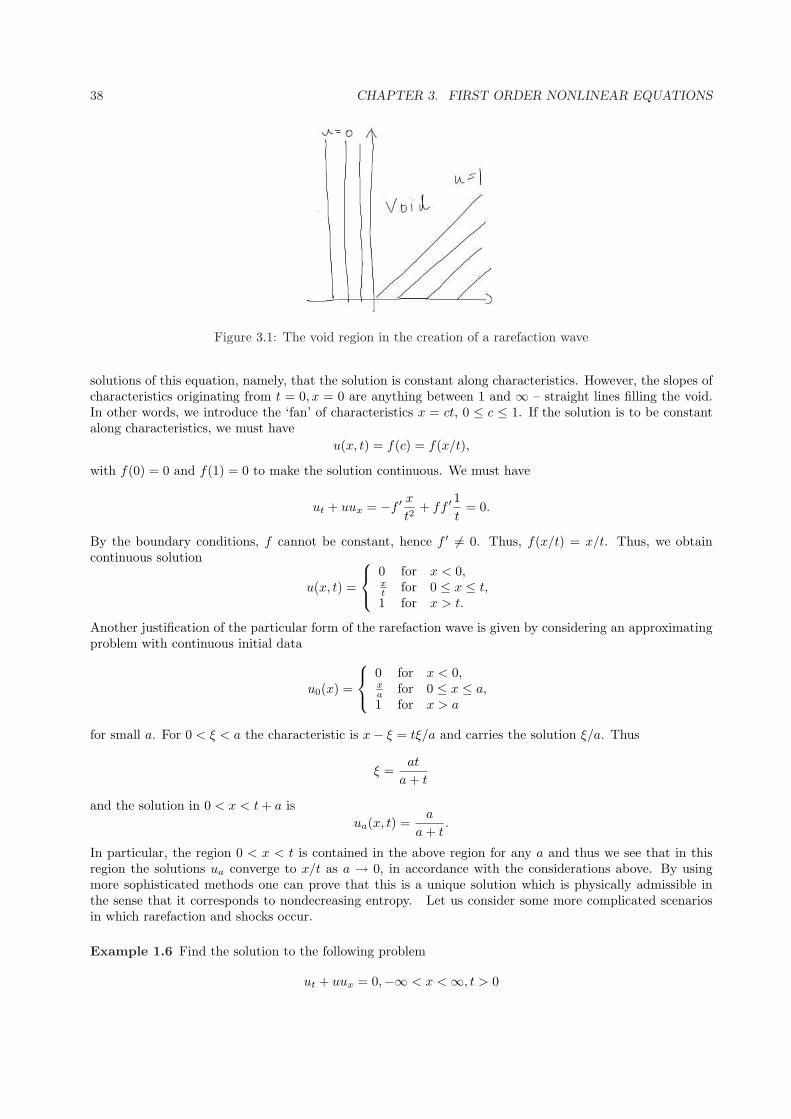
38 CHAPTER 3. FIRST ORDER NONLINEAR EQUATIONS
Figure 3.1: The void region in the creation of a rarefaction wave
solutions of this equation, namely, that the solution is constant along characteristics. However, the slopes ofcharacteristics originating from t = 0, x = 0 are anything between 1 and ∞ – straight lines filling the void.In other words, we introduce the ‘fan’ of characteristics x = ct, 0 ≤ c ≤ 1. If the solution is to be constantalong characteristics, we must have
u(x, t) = f(c) = f(x/t),
with f(0) = 0 and f(1) = 0 to make the solution continuous. We must have
ut + uux = −f ′x
t2+ ff ′
1t
= 0.
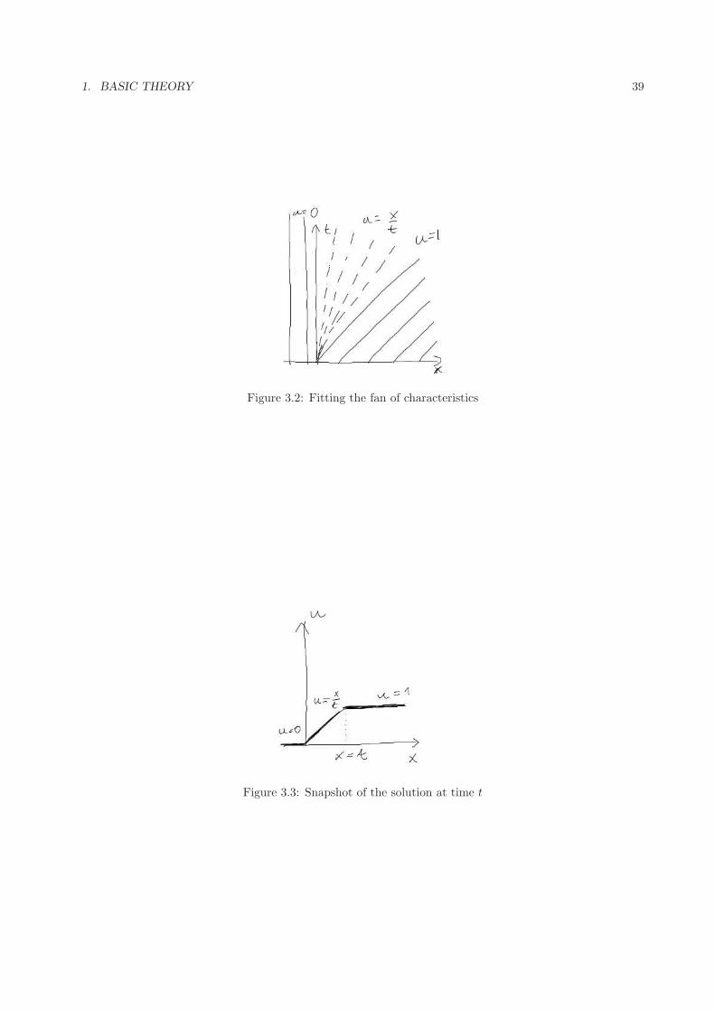
By the boundary conditions, f cannot be constant, hence f ′ 6= 0. Thus, f(x/t) = x/t. Thus, we obtaincontinuous solution
u(x, t) =
0 for x < 0,xt for 0 ≤ x ≤ t,1 for x > t.
Another justification of the particular form of the rarefaction wave is given by considering an approximatingproblem with continuous initial data
u0(x) =
0 for x < 0,xa for 0 ≤ x ≤ a,1 for x > a
for small a. For 0 < ξ < a the characteristic is x− ξ = tξ/a and carries the solution ξ/a. Thus
ξ =at
a + t
and the solution in 0 < x < t + a isua(x, t) =
a
a + t.
In particular, the region 0 < x < t is contained in the above region for any a and thus we see that in thisregion the solutions ua converge to x/t as a → 0, in accordance with the considerations above. By usingmore sophisticated methods one can prove that this is a unique solution which is physically admissible inthe sense that it corresponds to nondecreasing entropy. Let us consider some more complicated scenariosin which rarefaction and shocks occur.
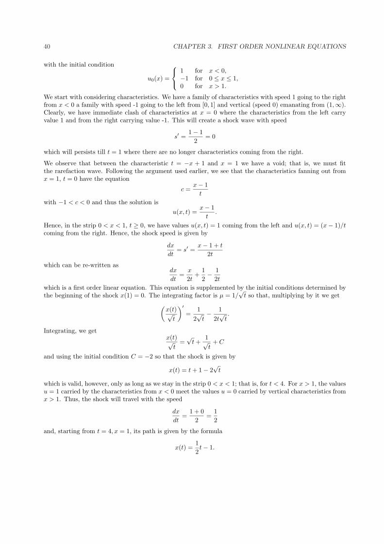
Example 1.6 Find the solution to the following problem
ut + uux = 0,−∞ < x < ∞, t > 0
1. BASIC THEORY 39
Figure 3.2: Fitting the fan of characteristics
Figure 3.3: Snapshot of the solution at time t
40 CHAPTER 3. FIRST ORDER NONLINEAR EQUATIONS
with the initial condition
u0(x) =
1 for x < 0,−1 for 0 ≤ x ≤ 1,0 for x > 1.
We start with considering characteristics. We have a family of characteristics with speed 1 going to the rightfrom x < 0 a family with speed -1 going to the left from [0, 1] and vertical (speed 0) emanating from (1,∞).Clearly, we have immediate clash of characteristics at x = 0 where the characteristics from the left carryvalue 1 and from the right carrying value -1. This will create a shock wave with speed
s′ =1− 1
2= 0
which will persists till t = 1 where there are no longer characteristics coming from the right.
We observe that between the characteristic t = −x + 1 and x = 1 we have a void; that is, we must fitthe rarefaction wave. Following the argument used earlier, we see that the characteristics fanning out fromx = 1, t = 0 have the equation
c =x− 1
t
with −1 < c < 0 and thus the solution isu(x, t) =
x− 1t
.
Hence, in the strip 0 < x < 1, t ≥ 0, we have values u(x, t) = 1 coming from the left and u(x, t) = (x− 1)/tcoming from the right. Hence, the shock speed is given by
dx
dt= s′ =
x− 1 + t
2t
which can be re-written asdx
dt=
x
2t+
12− 1
2t
which is a first order linear equation. This equation is supplemented by the initial conditions determined bythe beginning of the shock x(1) = 0. The integrating factor is µ = 1/
√t so that, multiplying by it we get
(x(t)√
t
)′=
12√
t− 1
2t√
t.
Integrating, we getx(t)√
t=√
t +1√t
+ C
and using the initial condition C = −2 so that the shock is given by
x(t) = t + 1− 2√
t
which is valid, however, only as long as we stay in the strip 0 < x < 1; that is, for t < 4. For x > 1, the valuesu = 1 carried by the characteristics from x < 0 meet the values u = 0 carried by vertical characteristics fromx > 1. Thus, the shock will travel with the speed
dx
dt=
1 + 02
=12
and, starting from t = 4, x = 1, its path is given by the formula
x(t) =12t− 1.
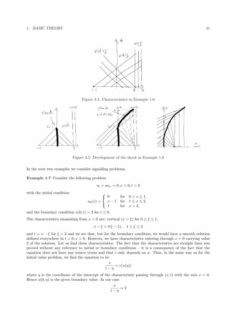
1. BASIC THEORY 41
Figure 3.4: Characteristics in Example 1.6
Figure 3.5: Development of the shock in Example 1.6
In the next two examples we consider signalling problems.
Example 1.7 Consider the following problem
ut + uux = 0, x > 0, t > 0
with the initial condition
u0(x) =
0 for 0 < x ≤ 1,x− 1 for 1 ≤ x ≤ 2,1 for x > 2,
and the boundary condition u(0, t) = 2 for t ≥ 0.
The characteristics emanating from x > 0 are: vertical (x = ξ) for 0 ≤ ξ ≤ 1,
x− ξ = t(ξ − 1), 1 ≤ ξ ≤ 2
and t = x− ξ for ξ > 2 and we see that, but for the boundary condition, we would have a smooth solutiondefined everywhere in t > 0, x > 0. However, we have characteristics entering through x = 0 carrying value2 of the solution. Let us find these characteristics. The fact that the characteristics are straight lines wasproved without any reference to initial or boundary conditions – it is a consequence of the fact that theequation does not have any source terms and that c only depends on u. Thus, in the same way as for theinitial value problem, we find the equation to be
x
t− η= c(u(η))
where η is the coordinate of the intercept of the characteristic passing through (x, t) with the axis x = 0.Hence u(0, η) is the given boundary value. In our case
x
t− η= 2
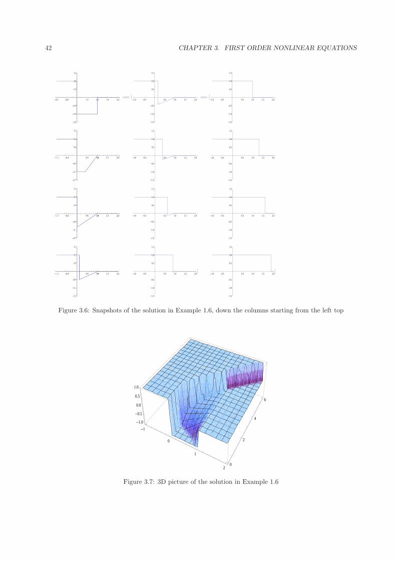
42 CHAPTER 3. FIRST ORDER NONLINEAR EQUATIONS
Out[21]= :-1.0 -0.5 0.5 1.0 1.5 2.0
-1.5
-1.0
-0.5
0.5
1.0
1.5
,
-1.0 -0.5 0.5 1.0 1.5 2.0
-1.5
-1.0
-0.5
0.5
1.0
1.5
,
-1.0 -0.5 0.5 1.0 1.5 2.0
-1.5
-1.0
-0.5
0.5
1.0
1.5
,
-1.0 -0.5 0.5 1.0 1.5 2.0
-1.5
-1.0
-0.5
0.5
1.0
1.5
>
Out[22]= :-1.0 -0.5 0.5 1.0 1.5 2.0
-1.5
-1.0
-0.5
0.5
1.0
1.5
,
-1.0 -0.5 0.5 1.0 1.5 2.0
-1.5
-1.0
-0.5
0.5
1.0
1.5
,
-1.0 -0.5 0.5 1.0 1.5 2.0
-1.5
-1.0
-0.5
0.5
1.0
1.5
,
-1.0 -0.5 0.5 1.0 1.5 2.0
-1.5
-1.0
-0.5
0.5
1.0
1.5
>
Figure 3.6: Snapshots of the solution in Example 1.6, down the columns starting from the left top
-1
0
1
20
2
4
6
-1.0
-0.5
0.0
0.5
1.0
Figure 3.7: 3D picture of the solution in Example 1.6
1. BASIC THEORY 43
and the equation of the characteristic is
t =12x + η.
It is clear that these characteristics clash with the characteristics immediately at t = 0 and thus the shockstarts at x = 0, t = 0. Since the characteristics entering from x = 0 carry the value 2 and the verticalcharacteristics from 0 < x < 1 carry the value 0, we immediately obtain the equation for the shock
dx
dt= s′ =
2 + 02
= 1
and so x(t) = t. This shock will continue until it reaches the the line x = 1 (at t = 1) whereupon in thefront of the wave we will have the value carried by the characteristics x − ξ = t(ξ − 1), 1 ≤ ξ ≤ 2. To findthese values, we solve for ξ:
ξ =t + x
t + 1so that the solution is
u(x, t) = u0(ξ) = ξ − 1 =x− 1t + 1
.
Thus, at the shock we would have
dx
dt=
2 + x−1t+1
2=
x
2(t + 1)+
2t + 12(t + 1)
which is a linear equation, which we supplement with the initial condition x = 1, t = 1 at the beginning ofthe shock. To simplify notation, let τ = t + 1 so that the equation becomes
x′ = x/2τ + 1− 1/2τ.
The integrating factor is 1/√
τ so that
(x/√
τ)′ = 1/√
τ − 1/(2τ√
τ)
and solving and returning to the original variables we get
x(t) = 2(t + 1) + 1 + C√
t + 1
and, using the initial condition, C = −4/√
2 hence
x(t) = 2t + 3− 4
√t + 1
2.
This shock continues till it reaches the characteristic t = x− 2; that is, until the time t which is the solutionto
2t + 3− 4
√t + 1
2= t + 2,
or t = 7. At this time the shock, still carrying the value 2 from the left, enters the region where thecharacteristics carry value 1 from the right and thus the shock’s speed is
s′(t) =2 + 1
2=
32
so that the shock’s path is
x(t) =32t + C
with C to be determined by the condition x = 9, t = 7 : 9 = 21/2 + C; that is, C = −3/2. Hence
x(t) =32t− 3
2.

44 CHAPTER 3. FIRST ORDER NONLINEAR EQUATIONS
Figure 3.8: Calculation of characteristics in a signalling problem
Figure 3.9: Characteristics in Example 1.7
Figure 3.10: Development of the shock in Example 1.7

1. BASIC THEORY 45
Example 1.8 Consider the following problem
ut + uux = 0, x > 0, t > 0
with the initial condition u0(x) = 1, x > 0 and the boundary condition u(0, t) = t + 1 for t ≥ 0.
We have characteristics t = x− ξ, ξ > 0 while the characteristics emanating from x = 0 are given implicitlyby
x
t− η= η + 1, η > 0
or−η2 + η(t− 1) + t− x = 0. (3.1.11)
The principle for determining the break time is the same as in the case of the initial value problem - for afixed characteristics we find time t for which the point (x(t), t) on this characteristic does not determine η ina unique way. In our case, the ‘ξ-characteristics’ always determine a unique ξ for any given (x, t). However,along the ‘η-characteristics’ we find that
0 = F (x, t, η) = −η2 + η(t− 1) + t− x
cannot be solved if0 = Fη(x, t, η) = −2η + t− 1
or t = 2η +1 (this gives the solvability region 0 < x < (t+1)2/4). The minimum over (0,∞) occurs at η = 0so that the breaking time is tb = 1. Thus, for 0 < t < 1 we can write the solution as
u(x, t) =
η(x, t) for 0 < x < t, 0 < t < 11 for x > t, 0 < t < 1,
where η(x, t) is given as the positive solution of (3.1.11); that is,
η(x, t) =t− 1 +
√(t− 1)2 + 4(t− x)
2. (3.1.12)
Let us find the equation of the shock wave. The shock will have values transported by ‘η-characteristics’from the left and ‘ξ-characteristics’ from the right; that is
dx
dt= s′(t) =
η(x, t) + 12
. (3.1.13)
However, substituting η found above into this expression creates a formidable equation which seems to beimpossible to solve directly. Since the right hand side appears relatively simple, let us try to express dx/dtin terms of dη/dt. Differentiating (3.1.11) implicitly with respect to t, we get
−2ηηt + ηt(t− 1) + η + 1− xt = 0
orxt = ηt(t− 2ηt − 1) + η + 1.
Substituting into (3.1.13) and simplifying, we obtain
dη
dt=
η
2(2η − (t− 1)).
This equation simplifies if we assume dη/dt 6= 0 (that is, η 6= 0). Then we can treat η as the independentvariable t = t(η) and, substituting τ = t− 1, we get
dτ
dη= 4− 2τ
η(3.1.14)
46 CHAPTER 3. FIRST ORDER NONLINEAR EQUATIONS
which is a linear ordinary differential equation. We see that the integrating factor is µ = η2 so that
(η2τ)′ = 4η2
that isη2τ =
43η3 + C. (3.1.15)
Now, the shock starts at x = 1, t = 1 or η = 0, τ = 0 which is outside the range for which the equation isvalid. However, if we insists that the above solution is valid as η → 0 and τ → 0, we arrive at C = 0. Fornonzero η we get
η =34(t− 1)
and, substituting to (3.1.11), we find
x(t) = (1− η)(η − 1) =(
34(t− 1) + 1
)(t− 3
4(t− 1)
)=
116
(3t + 1)(t + 3). (3.1.16)
We note that up to now the process has been purely formal - we are not sure that all the assumptions for theperformed transformations to be correct are satisfied. However, we can validate the process of obtaining thesolution by first checking that it fits into the region where ηt is defined: t < x < (t + 1)2/4 and substitutingthe above function defined (3.1.16) into (3.1.12) to ascertain that indeed it is a solution. The questionremains whether (3.1.16) is the only solution. We note that (1, 1) is the singular point of (3.1.12) where theassumptions of the Picard theorem are not satisfied and thus there may be other solutions. However, weobserve that in the open region t < x < (t + 1)2/4 the equations (3.1.12) and (3.1.14) are equivalent andthus any solution in this region is given by (3.1.15). If we want this solution to converge to (η, τ) = (0, 0) wemust have C = 0 and thus the solution x(t) we obtained is the only solution in the region t < x < (t + 1)2/4satisfying x(1) = 1.
2 Application to traffic flow
We illustrate the ideas introduced above to the classical model of one dimensional traffic flow.
Imagine a long stretch of narrow straight road with heavy traffic. Then, instead of considering separate carswe can talk about a traffic flow by introducing the traffic density ρ which is the number of vehicles per unitlength of the road and, instead of considering the speed of a particular car, we can consider the speed u(x, t)of traffic at a particular point x and time t. Related to it is the traffic flow φ(x) at x defined, as usual, asthe number of cars passing through x at time t per unit time. It is easy to see that, for an observer sittingat x, over a short time ∆t the traffic will move by the length u∆t but in this length we have ρu∆t vehicles.Thus, in unit time on average we will have the flux
φ = uρ
at x and t. Assuming that no new cars enter the road nor vanish from it, we have the conservation law
d
dt
b∫
a
ρ(x, t)dx = φ(a, t)− φ(b, t),
or, under assumption that u and φ are differentiable,
ρt + φx = 0. (3.2.17)
Our considerations will be carried out under simplifying assumption that the flux only depends on the densityof traffic
φ = φ(ρ)
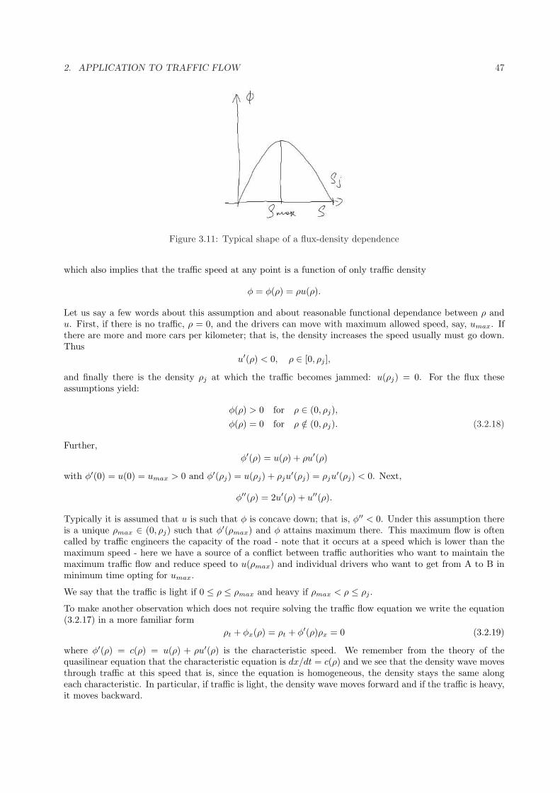
2. APPLICATION TO TRAFFIC FLOW 47
Figure 3.11: Typical shape of a flux-density dependence
which also implies that the traffic speed at any point is a function of only traffic density
φ = φ(ρ) = ρu(ρ).
Let us say a few words about this assumption and about reasonable functional dependance between ρ andu. First, if there is no traffic, ρ = 0, and the drivers can move with maximum allowed speed, say, umax. Ifthere are more and more cars per kilometer; that is, the density increases the speed usually must go down.Thus
u′(ρ) < 0, ρ ∈ [0, ρj ],
and finally there is the density ρj at which the traffic becomes jammed: u(ρj) = 0. For the flux theseassumptions yield:
φ(ρ) > 0 for ρ ∈ (0, ρj),φ(ρ) = 0 for ρ /∈ (0, ρj). (3.2.18)
Further,φ′(ρ) = u(ρ) + ρu′(ρ)
with φ′(0) = u(0) = umax > 0 and φ′(ρj) = u(ρj) + ρju′(ρj) = ρju
′(ρj) < 0. Next,
φ′′(ρ) = 2u′(ρ) + u′′(ρ).
Typically it is assumed that u is such that φ is concave down; that is, φ′′ < 0. Under this assumption thereis a unique ρmax ∈ (0, ρj) such that φ′(ρmax) and φ attains maximum there. This maximum flow is oftencalled by traffic engineers the capacity of the road - note that it occurs at a speed which is lower than themaximum speed - here we have a source of a conflict between traffic authorities who want to maintain themaximum traffic flow and reduce speed to u(ρmax) and individual drivers who want to get from A to B inminimum time opting for umax.
We say that the traffic is light if 0 ≤ ρ ≤ ρmax and heavy if ρmax < ρ ≤ ρj .
To make another observation which does not require solving the traffic flow equation we write the equation(3.2.17) in a more familiar form
ρt + φx(ρ) = ρt + φ′(ρ)ρx = 0 (3.2.19)
where φ′(ρ) = c(ρ) = u(ρ) + ρu′(ρ) is the characteristic speed. We remember from the theory of thequasilinear equation that the characteristic equation is dx/dt = c(ρ) and we see that the density wave movesthrough traffic at this speed that is, since the equation is homogeneous, the density stays the same alongeach characteristic. In particular, if traffic is light, the density wave moves forward and if the traffic is heavy,it moves backward.

48 CHAPTER 3. FIRST ORDER NONLINEAR EQUATIONS
It is important to realize here that we have two speeds involved in the model - the traffic speed and thespeed of the density wave (the speed with which the signal propagates through traffic). Now
c(ρ) = u(ρ) + ρu′(ρ) < u(ρ)
on account of u′ being a decreasing function, thus the density wave travels slower than the traffic.
In the following examples we shall take a simple linear speed-density dependance
u(ρ) = umax
(1− ρ
ρj
)
yielding
φ(ρ) = umaxρ
(1− ρ
ρj
)
It is easy to see that the characteristic speed is
c(ρ) = φ′(ρ) = umax
(1− 2ρ
ρj
).
In other words, we will be working with the equation
ρt + umax
(1− 2ρ
ρj
)ρx = 0 (3.2.20)
From the expression for φ′ we see that the maximum flow occurs at ρmax = ρj/2 corresponding to theoptimal speed umax/2.
We can simplify the equation by introducing a dimensionless density g = ρ/ρj . We also shorten notation bydenoting umax = υ. Then the equation turns into
gt + υ (1− 2g) gx = 0, (3.2.21)
with 0 ≤ g ≤ 1.
Example 2.1 Consider the following problem. It is observed that at a red light at an intersection a typicalqueue of cars is of length x0 with no traffic behind the back of the queue and no traffic in front of the trafficlights. What should be the green phase to allow all cars in the queue pass the intersection.
We assume that the traffic obeys Eq. (3.2.23) and that the traffic lights are at x = 0. The fact that the carsdo not move in front of the red light is modelled by the initial condition
g0(x) =
0 for x < −x0,1 for −x0 < x < 0,0 for x > 0,
(recall that g = 1 corresponds to the maximum density.) To solve the problem, first we find characteristics.Observe that contrary to the previous examples, here we have c(g) = υ(1 − 2g) and thus the characteristicspeed is υ for ξ < −x0 and ξ > 0 and −υ for −x0 < ξ < 0. Hence, we have the following families ofcharacteristics x − ξ = υt for ξ < −x0 and x > 0 and x − ξ = −υt for −x0 < ξ < 0. Therefore we havea rarefaction wave originating at x = 0, t = 0 and a shock wave originating at x = −x0 and t = 0. Inthis model the interpretation of these waves is simply that in the front of the queue cars immediately startmoving with the maximum velocity υ (as there is no traffic in front and the shock wave corresponds to thediscontinuity between the back of the queue and the no traffic zone behind the queue). Mathematically, thefan of characteristics is given by x/t = c(ρ) with −υ < c(ρ) < υ but here c is given by
c(g) = υ(1− 2g)
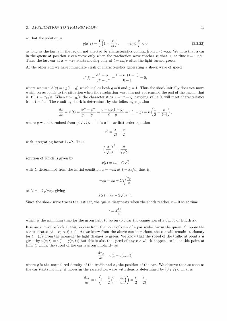
2. APPLICATION TO TRAFFIC FLOW 49
so that the solution isg(x, t) =
12
(1− x
υt
), −υ <
x
t< υ (3.2.22)
as long as the fan is in the region not affected by characteristics coming from x < −x0. We note that a carin the queue at position x can move only when the rarefaction wave reaches x; that is, at time t = −x/υ.Thus, the last car at x = −x0 starts moving only at t = x0/υ after the light turned green.
At the other end we have immediate clash of characteristics generating a shock wave of speed
s′(t) =φ+ − φ−
g+ − g−=
0− υ1(1− 1)0− 1
= 0,
where we used φ(g) = υg(1− g) which is 0 at both g = 0 and g = 1. Thus the shock initially does not movewhich corresponds to the situation when the rarefaction wave has not yet reached the end of the queue; thatis, till t = x0/υ. When t > x0/υ the characteristics x − υt = ξ, carrying value 0, will meet characteristicsfrom the fan. The resulting shock is determined by the following equation
dx
dt= s′(t) =
φ+ − φ−
g+ − g−=
0− υg(1− g)0− g
= υ(1− g) = υ
(12− x
2υt
),
where g was determined from (3.2.22). This is a linear first order equation
x′ =x
2t+
υ
2
with integrating factor 1/√
t. Thus (x√t
)′=
υ
2√
t
solution of which is given byx(t) = υt + C
√t
with C determined from the initial condition x = −x0 at t = x0/υ, that is,
−x0 = x0 + C
√x0
υ
or C = −2√
υx0, givingx(t) = υt− 2
√υx0t.
Since the shock wave traces the last car, the queue disappears when the shock reaches x = 0 so at time
t = 4x0
υ
which is the minimum time for the green light to be on to clear the congestion of a queue of length x0.
It is instructive to look at this process from the point of view of a particular car in the queue. Suppose thecar is located at −x0 < ξ < 0. As we know from the above considerations, the car will remain stationaryfor t = ξ/υ from the moment the light changes to green. We know that the speed of the traffic at point x isgiven by u(x, t) = υ(1 − g(x, t)) but this is also the speed of any car which happens to be at this point attime t. Thus, the speed of the car is given implicitly as
dxc
dt= υ(1− g(xc, t))
where g is the normalized density of the traffic and xc the position of the car. We observe that as soon asthe car starts moving, it moves in the rarefaction wave with density determined by (3.2.22). That is
dxc
dt= υ
(1− 1
2
(1− xc
υt
))=
υ
2+
xc
2t
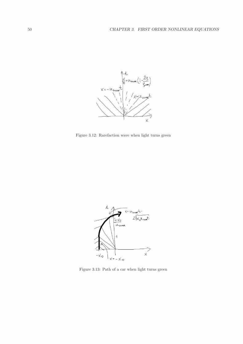
50 CHAPTER 3. FIRST ORDER NONLINEAR EQUATIONS
Figure 3.12: Rarefaction wave when light turns green
Figure 3.13: Path of a car when light turns green
2. APPLICATION TO TRAFFIC FLOW 51
which is exactly the differential equation of the shock wave (which we interpreted as the trajectory of thelast car in the queue), only with different initial conditions. This gives the trajectory of the car
xc(t) = υt− 2√−υξt,
(remember ξ < 0) and the time when the car passes the lights is t = −4ξ/υ.
Next we consider what happens when the light turns red.
Example 2.2 Consider a uniform traffic moving to the right with (normalized) density g0 < 1. Assumethat at t = 0 the traffic light at x = 0 turns red. To model this we note that when the lights are red, themoving cars must stop and cars do not move only when g = 1 (ρ = ρmax). Thus, the traffic behind the lightscan be modelled by the signalling problem
gt + υ (1− 2g) gx = 0, x < 0, t > 0 (3.2.23)
andg(x, 0) = g0, x < 0, g(0, t) = 1, 0 < t < t0
where t0 is the length of the red phase. Then the characteristics emanating from x < 0 are given by
x− ξ = tc(g0) = tυ(1− 2g0)
whereas from x = 0 byx = (t− η)c(1) = υ(t− η).
Depending on whether the traffic is heavy (g0 > 1/2) or light (g0 < 1/2), the characteristic speed of ‘ξ′-characteristics is, respectively, negative or positive, but in both cases υ (1− 2g) > −υ which means thatthe ‘ξ′-characteristics are steeper than the ‘η′-characteristics and therefore we observe creation of a shockoriginating from t = 0 and x = 0. In this case the position of the shock indicated the point to the right ofwhich the traffic is already jammed and to the left it is still moving. The shock speed is given as before by
dx
dt= s′(t) =
φ+ − φ−
g+ − g−=
0− g0u(g0)1− g0
=0− υg0(1− g0)
1− g0= −υg0,
and the shock path is given byx(t) = −υg0t. (3.2.24)
As before, we can look at this problem from the point of view of an individual car which is at a distance ξfrom the origin when the light turns red. Here it is better to use the real density ρ0 and not the normalizedone. Since the density of traffic is uniform, we have approximately N = ξρ0 cars between our car and thetraffic light. The car will stop at the point −ξ1 such that the density on [−ξ1, 0] is ρj . Thus, we must haveρj = N/ξ1. Solving for N we obtain
ξ1 = ξρ0/ρj .
On the other hand, since the density, and hence the traffic speed, is uniform, the path between −ξ and −ξ1
is covered in t = (ξ − ξ1)/u(ρ0). Denoting −ξ1 = x(t) and eliminating ξ we have
x(t) =ρ0
ρj(u(ρ0)t + x(t))
which, due to u(ρ0) = υ(1− ρ0/ρj), yields
x(t) = −υρ0
ρjt = −υg0t,
in perfect agreement with (3.2.24).

52 CHAPTER 3. FIRST ORDER NONLINEAR EQUATIONS
Figure 3.14: Characteristics for heavy traffic (left) and light traffic (right)
Figure 3.15: Shock path when light turns red
3 An exactly solvable McKendrick nonlinear model
In Subsection 1.1 we introduced the age structured McKendrick population model
∂n(a, t)∂t
+∂n(a, t)
∂a= −µ(a, t)n(a, t), t, a > 0
n(0, t) =
∞∫
0
n(a, t)m(a, t)da, t > 0,
n(a, 0) = n0(a), a > 0
where µ is the death rate, m is the maternity rate and∞ is the maximum age of individuals in the population.
In many cases the assumption that µ and m do not depend on the population is an oversimplification. Amore realistic system
∂n(a, t)∂t
+∂n(a, t)
∂a= −µ(a, t,N)n(a, t), t, a > 0
n(0, t) =
∞∫
0
n(a, t)m(a, t, N)da, t > 0,
n(a, 0) = n0(a), a > 0 (3.3.25)
where
N(t) =
∞∫
0
n(a, t)da
3. AN EXACTLY SOLVABLE MCKENDRICK NONLINEAR MODEL 53
is the total population at time t. This makes (3.3.25) a (badly) nonlinear equation which only can be solvedin very special cases. We shall describe one such case. Consider
∂n(a, t)∂t
+∂n(a, t)
∂a= −µ0N(t)n(a, t), t, a > 0
n(0, t) =
∞∫
0
n(a, t)m0N(t)da, t > 0,
n(a, 0) = n0(a), a > 0 (3.3.26)
where µ0,m0 are positive constants. Let us integrate the first and second equation with respect to a. Letus start with observing that
∞∫
0
na(a, t)da = lima→∞
n(a, t)− n(0, t) = −m0N
∞∫
0
n(a, t)da− 0 = −m0N2(t),
where we used lima→∞ n(a, t) = 0 which reflects the the assumption that the number of individuals survivingtill an old age is decreasing to 0. Thus, integration of the first and the last equation in (3.3.28) yields
Nt = N2(m0 − µ0), N(0) = N0 =
∞∫
0
n0(a)da. (3.3.27)
There are two cases to consider.
a) µ0 = m0.In this case, N(t) = N0 for all t ≥ 0 and (3.3.28) turns into
∂n(a, t)∂t
+∂n(a, t)
∂a= −µ0N0n(a, t), t, a > 0
n(0, t) =
∞∫
0
n(a, t)m0N0da, t > 0,
n(a, 0) = n0(a), a > 0 (3.3.28)
which is of the form (2.1.18). We could use the formula which we derived there but here we can use the factthat
n(0, t) =
∞∫
0
n(a, t)m0N0da = m0N0
∞∫
0
n(a, t)da = m0N0N(t) = m0N20
and we deal with a straightforward initial boundary value problem
∂n(a, t)∂t
+∂n(a, t)
∂a= −µ0N0n(a, t), t, a > 0
n(0, t) = m0N20 , t > 0,
n(a, 0) = n0(a), a > 0 (3.3.29)
the solution of which is given by (2.1.19)
n(a, t) = e−m0N0au(a, t) = e−m0N0a
em0N0(a−t)n0(a− t), t < a,m0N
20 , a < t
=
e−m0N0tn0(a− t), t < a,e−m0N0am0N
20 , a < t.
(3.3.30)
54 CHAPTER 3. FIRST ORDER NONLINEAR EQUATIONS
b) µ0 6= m0.In this case the solution of (3.3.27) is given by
1N0
− 1N(t)
= (m0 − µ0)t
orN(t) =
N0
1− (m0 − µ0)N0t. (3.3.31)
At this moment we note that the evolution of the population is determined by the sign of r0 = m0−µ0 whichplays the role of the net growth rate: if r0 > 0 (that is, if the maternity coefficient exceeds the mortalityrate), the population will explode at t = 1/(r0)N0. On the other hand, if r0 < 0 (that is, if the maternitycoefficient is lower than the mortality rate), the population will exists for all time gradually decaying to 0.However, in both cases we can give explicit formulae for n(a, t). Indeed, similarly to a) we arrive at thestraightforward initial boundary value problem
∂n(a, t)∂t
+∂n(a, t)
∂a= −µ0N(t)n(a, t), t, a > 0
n(0, t) = m0N(t)2, t > 0,
n(a, 0) = n0(a), a > 0 (3.3.32)
where N(t) is given (3.3.31). However, contrary to (3.3.29) (and (2.1.18)), the coefficient µ is dependent ontime and thus the reduction must be made with more care. We begin by noting that
d
dteµ0
t∫0
N(s)ds= m0N(t)e
µ0
t∫0
N(s)ds
and thus the first equation of (3.3.32) can be written as
∂
∂t
n(a, t)e
µ0
t∫0
N(s)ds
+
∂
∂a
n(a, t)e
µ0
t∫0
N(s)ds
= 0.
If we denote
u(a, t) = n(a, t)eµ0
t∫0
N(s)ds
then
u(a, 0) = n(a, 0)eµ0
0∫0
N(s)ds= n0(a)
and
u(0, t) = n(0, t)eµ0
t∫0
N(s)ds= m0N(t)2e
µ0
t∫0
N(s)ds
so that, using again (2.1.19), we obtain
n(a, t) = e−µ0
t∫0
N(s)dsu(a, t) = e
−µ0
t∫0
N(s)ds
n0(a− t), t < a,
m0N(t− a)2eµ0
t−a∫0
N(s)ds, a < t
=
e−µ0
t∫0
N(s)dsn0(a− t), t < a,
m0N(t− a)2e−µ0
t∫t−a
N(s)ds
, a < t
(3.3.33)
as long as N is defined. For our particular case we have
∫N(s)ds = N0
∫ds
1− r0N0t= ln
(1
1−N0r0t
) 1r0
+ C
3. AN EXACTLY SOLVABLE MCKENDRICK NONLINEAR MODEL 55
for 0 ≤ t < 1/r0N0 if r0 > 0 and for 0 ≤ t < ∞ otherwise. Hence, for such t
e−µ0
t∫0
N(s)ds= (1− r0N0t)
µ0r0
and
e−µ0
t∫t−a
N(s)ds
=(
1− r0N0t
1− r0N0(t− a)
)µ0r0
.
Thus
n(a, t) =
(1− r0N0t)µ0r0 n0(a− t), t < a,
m0N20
(1−r0N0(t−a))2
(1−r0N0t
1−r0N0(t−a)
)µ0r0
, a < t.

56 CHAPTER 3. FIRST ORDER NONLINEAR EQUATIONS
Chapter 4
Similarity methods for linear andnon-linear diffusion
1 Similarity method
The method described in this section can be applied to equations of arbitrary order. However, having inmind concrete application we shall focus on the general second order partial differential equation in twoindependent variables in the form
G(t, x, u, ux, ut, uxx, uxt, utt) = 0. (4.1.1)
To shorten notation we introduce notation
p = ux, q = ut, r = uxx, s = uxt, v = utt.
We introduce the one-parameter family of stretching transformations, denoted by Tε, by
x = εax, t = εbt, u = εcu (4.1.2)
where a, b, c are real constants and ε is a real parameter restricted to some open interval I containing ε = 1.We note that (4.1.2) induces a transformation of the derivatives in the following way:
p =∂u
∂x= εc ∂u
∂x
dx
dx= εc−ap (4.1.3)
and similarly for other derivatives
q = εc−bq, r = εc−2ar, s = εc−a−bs, v = εc−2bv. (4.1.4)
Further, we say that PDE (4.1.1) is invariant under the one parameter family Tε of stretching transformationsif there exists a smooth function f(ε) such that
G(t, x, u, p, q, r, s, v) = f(ε)G(t, x, u, p, q, r, s, v) (4.1.5)
for all ε ∈ I, with f(1) = 1. If f(ε) ≡ 1 for all ε ∈ I, then the PDE (4.1.1) is said to be absolutely invariant.
We shall formulate and prove the fundamental theorem.
Theorem 1.1 If the equation (4.1.1) is invariant under the family Tε defined by (4.1.2), then the transfor-mation
u = tc/by(z), z =x
ta/b(4.1.6)
reduces (4.1.1) to a second order ordinary differential equation in y(z).
57

58 CHAPTER 4. SIMILARITY METHODS FOR LINEAR AND NON-LINEAR DIFFUSION
Proof. By invariance, we know that (4.1.5) holds for all ε in some open interval containing 1 thus we candifferentiate (4.1.5) and set ε = 1 after differentiation getting
axGx + btGt + cuGu + (c− a)pGp + (c− b)qGq + (c− 2a)rGr + (c− a− b)sGs + (c− 2b)vGv = f ′(1)G
where we used formulae likedx
dε
∣∣∣∣ε=1
= aεa−1x∣∣ε=1
= ax,
etc. The above equation is a first order equation so that we can integrate it using t as the parameter alongcharacteristics. The characteristic system will be then
dG
dt=
f ′(1)Gbt
dx
dt=
ax
btdu
dt=
cu
btdp
dt=
(c− a)pbt
dq
dt=
(c− b)qbt
dr
dt=
(c− 2a)rbt
ds
dt=
(c− a− b)sbt
dv
dt=
(c− 2b)vbt
Thus, we obtain characteristics defined by
xt−a/b = z,
ut−c/b = ξ1, pt−(c−a)/b = ξ2, qt−(c−b)/b = ξ3,
rt−(c−2a)/b = ξ4, st−(c−a−b)/b = ξ5, vt−(c−2b)/b = ξ6
and
G = tf′(1)bΨ(z, ξ1, ξ2, ξ3, ξ4, ξ5, ξ6) (4.1.7)
where Ψ is an arbitrary function. Now, we have y = ut−c/b = ξ1, p = ux = tc/by′zz′x = y′zt
(c−a)/b, henceξ2 = y′z. Further,
q = ut =c
bt−1+c/by − a
btc/b−a/b−1xy′z,
thus
ξ3 = qt1−c/b =c
by − a
bzy′z.
Further,
r = uxx = px = y′′zzt(c−a)/bz′x = y′′zzt
(c−2a)/b,
hence ξ4 = y′′zz. Similarly,
s = utx = qx =c
bt−1+c/by′zz
′x −
a
btc/b−a/b−1y′z −
a
btc/b−a/b−1y′′zzz
′x = tc/b−a/b−1
(c− a
by′z −
a
by′′zzz
)
2. LINEAR DIFFUSION EQUATION 59
giving ξ5 = c−ab y′z − a
b y′′zzz and finally
v = qt =c
b
(c
b− 1
)t−2+c/by +
c
bt−1+c/by′zz
′t
−a
b
((c
b− 1
)t−2+c/bzy′z + t−1+c/bz′ty
′z + t−1+c/bzy′′zzz
′t
)
= t−2+c/b(c
b
((c
b− 1
)y − a
bzy′z
)− a
b
((c
b− 1
)zy′z −
a
bzy′z −
a
bz2y′′zz
))
= t−2+c/b
(c
b
(c
b− 1
)y − 2
ac
b2zy′z +
a
bzy′z +
a2
b2zy′z +
a2
b2z2y′′zz
)
so that
ξ6 =c
b
(c
b− 1
)y − a
b
(2c
b− 1− a
b
)zy′z +
a2
b2z2y′′zz
Hence, combining (4.1.7) with the original equation (4.1.1) we obtain
Ψ(
z, y, y′,c
by − a
bzy′z, y
′′zz,
c− a
by′z −
a
by′′zzz,
c
b
(c
b− 1
)y − a
b
(2c
b− 1− a
b
)zy′z +
a2
b2z2y′′zz
)= 0
which is a second order ordinary differential equation in z.
2 Linear diffusion equation
Consider the diffusion equationut −Duxx. (4.2.1)
We shall try to find a stretching transformation under which this equation is invariant. Using our simplifiednotation for derivatives we have
q −Dr = εc−bq −Dεc−2ar.
We achieve invariance if ε is risen to the same power. Thus, we must have
b = 2a
with c and a at this moment arbitrary. Thus, (4.2.1) is invariant under the stretching transformation
x = εa, t = ε2at, u = εcu (4.2.2)
and the similarity transformation is given by
u = tc/2ay(z), z =x√t. (4.2.3)
We have z′x = 1√t, z′t = − 1
2xt−3/2 = − 12zt−1, hence
ut = − c
2at−1+c/2ay + tc/2ay′zz
′t = −t−1+c/2a
( c
2ay − z
2y′z
)
andux = tc/2a−1/2y′z, uxx = tc/2a−1y′′zz.
Substituting the above relations into the diffusion equation yields
Dy′′ +z
2y′ − c
2ay = 0. (4.2.4)
Constants c and a are in general arbitrary.
An important comment is in place here. Though the diffusion equation has been reduced to an ordinarydifferential equation, one should not think that any problem related to the diffusion equation is reducible to
60 CHAPTER 4. SIMILARITY METHODS FOR LINEAR AND NON-LINEAR DIFFUSION
an ODE problem so the similarity approach by no means solves all PDE problems. In fact, an inherent partof a diffusion problem are initial and boundary conditions and these, in general, cannot be translated intoside conditions for (4.2.4). For instance, consider the initial value problem for the diffusion equation
ut = Duxx, t > 0,−∞ < x < ∞,
u(x, 0) = u0(x). (4.2.5)
Using the similarity transformation, we can convert the equation into an ODE for f defined as u(x, t) =tc/2ay(x/
√t) but then putting t = 0 in the preceding formula in general does not make any sense as, at best,
we would have something like
y(∞) = limt→0+
t−c/2au(x, t), x > 0,
y(−∞) = limt→0+
t−c/2au(x, t), x < 0, (4.2.6)
with the right hand side equal to 0 if c/2a < 0, ∞ if c/2a > 0 or u0(x) if c = 0. Now, in the first two casesall the information coming from the initial condition is lost and the last one imposes a strict condition on u0:u0 must be constant on each semi-axis. Note that such a condition is also invariant under the transformationz = x/
√t: z ≶ 0 if and only if x ≶ 0. In general, the similarity method provides a full solution to the
initial-boundary value problems only if the side conditions are also invariant under the same transformationor, in other words, can be expressed in terms of the similarity variable. Otherwise, this method can serve asa first step in building more general solution, as we shall see below.
Consider the initial value problem
ut = Duxx, t > 0,−∞ < x < ∞,
u(x, 0) = H(x) (4.2.7)
where H is the Heaviside function: H(x) = 1 for x ≥ 0 and H(x) = 0 for x < 0. According to the discussionabove, this initial condition yields to the similarity method provided c = 0; in this case a is irrelevant andwe put it equal to 1. Thus, the initial value problem (4.2.7) is transformed into
y′′ +z
2Dy′ = 0,
y(−∞) = 0, y(∞) = 1. (4.2.8)
Denoting y′ = h, we reduce the equation to the first order equation
h′ +z
2Dh = 0
which can be integrated to y′ = h = c1 exp(−z2/4D). Integrating this once again, we obtain
y(z) = c1
z∫
0
e−η2
4D dη + c2 (4.2.9)
and the constants c1 and c2 can be obtained from the initial conditions
1 = limz→+∞
y(z) = c1
∞∫
0
e−η2
4D dη + c2 =√
4Dc1
∞∫
0
e−s2ds + c2 = c1
√4Dπ
2+ c2,
0 = limz→−∞
y(z) = c1
−∞∫
0
e−η2
4D dη + c2 =√
4Dc1
−∞∫
0
e−s2ds + c2 = −c1
√4Dπ
2+ c2,
where we used∞∫0
e−s2ds =
√π/2, so that
c2 =12, c1 =
1√4πD
.
3. NONLINEAR DIFFUSION MODELS 61
Hence
u(x, t) = y
(x√t
)=
12
+1√4πD
x√t∫
0
e−η2
4D dη (4.2.10)
The fundamental role in the theory of the diffusion equation is played by the derivative of u with respect tox:
S(x, t) =∂u
∂x(x, t) =
1√4πDt
e−x24Dt (4.2.11)
that is called source function or fundamental solution of the diffusion equation.
The reason for the importance of the fundamental solution is that it describes diffusion of a unit quantityof the medium concentrated at the origin and thus provides the solution to the initial value problem for thediffusion equation of the form
ut = Duxx,
u(x, 0) = δ(x)
where δ(x) is Dirac’s delta ”function”. One can check that S(x, t) has the following properties:
limt→0+
S(x, t) = 0, x 6= 0, (4.2.12)
limt→0+
S(x, t) = ∞, x = 0, (4.2.13)
limx→±∞
S(x, t) = 0, x > 0, (4.2.14)
∞∫
−∞S(x, t)dx = 1, t > 0, (4.2.15)
In general, it can be proved that the initial value problem (4.2.5) has a unique solution given by
u(x, t) =
∞∫
−∞S(x− ξ)u0(ξ)dξ (4.2.16)
provided u0 is sufficiently regular (e.g. bounded and continuous).
3 Nonlinear diffusion models
The linear diffusion equation, though extremely useful and important in applications, has at least one majordrawback - it is physically incorrect as it admits infinite speed of signal transmission. To alleviate thisproblem a number of nonlinear versions of this equation has been presented and we shall discuss some ofthem.
3.1 Models
Let us recall that the starting point for the derivation of the diffusion equation was the conservation law
ut + φx = 0 (4.3.1)
and the linear equation was obtained by postulating the flux in the form of Fick’s law
φ = −Dux. (4.3.2)
62 CHAPTER 4. SIMILARITY METHODS FOR LINEAR AND NON-LINEAR DIFFUSION
In population models usually there is the increase in diffusion due to the population pressure and it is thenreasonable to assume that the coefficient D itself should depend on the density u, that is,
φ = −D(u)ux (4.3.3)
and substituting this to the conservation law (4.3.1) yields the nonlinear equation
ut = (D(u)ux)x. (4.3.4)
Another place where the nonlinearity can occur is at the time derivative. For instance, deriving the heatequation we start with the energy conservation law
(ρCT )t + φx = 0 (4.3.5)
where T is the temperature, ρ is the density and C is the specific heat of the medium (so that the first termsdescribes the rate of change of the amount of energy contained in a unit volume). The flux φ is given by theFourier law
φ = −KTx,
where K is thermal conductivity of the medium. In many applications, where the temperature range islimited, the specific heat and the density may be regarded as constants. However, over a wide temperatureranges, they are not constants but rather depend on the temperature and in this case (4.3.5) combined withFourier’s law give the equation
(ρ(T )C(T )T )t = KTxx, (4.3.6)
which is a nonlinear diffusion equation for the temperature T .
These two types of nonlinearities can, of course, appear in a single equation. Consider, for instance, theporous medium equation, where we wish to describe a fluid (e.g. water) seeping downward through the soil.Let ρ(x, t) be the density of the fluid, with positive x measured downward. In a given volume of soil only afraction of the space is available to the fluid, the remaining being reserved for the soil itself. If the fractionof the volume that is available to the fluid is denoted by κ, then mass balance for the fluid can be written as
κρt + (ρv)x = 0, (4.3.7)
where we used the formula φ = vρ with v being the volumetric flow rate (velocity of the flow). Theconservation law (4.3.7) contains two unknowns: the density and the velocity of the flow so we need anotherconstitutive equation relating them. Without going through too much of physics we state that in many casesthe constitutive relation
v = aργx
for some constants γ > 1, a > 0. Thus, the porous media equation can be written as
κρt = a(ρργx)x = aγ(ργρx)x = αρm
xx (4.3.8)
where α = aγ/(γ + 1) and m = γ + 1 > 2. Since, in general, κ can be ρ-dependent, the porous mediaequation combines nonlinearities of (4.3.6) and (4.3.4) (with D(ρ) = aγργ .)
3.2 Some solutions
Let us consider a special case of Eq. (4.3.4) with D(u) = u, that is,
ut − (uux)x = 0. (4.3.9)
To compare the nonlinear equation with the linear diffusion, we shall try to solve it on R subject to theinitial condition of a unit point source applied at x = 0, that is,
u(x, 0) = δ(x).
3. NONLINEAR DIFFUSION MODELS 63
To simplify considerations we shall change this condition into two, more amenable to the similarity method,so that we shall look for solutions satisfying
∞∫
−∞u(x, t)dx = 1, t > 0 (4.3.10)
andlim
x→±∞= 0. (4.3.11)
As follows from Eqs. (4.2.12)–(4.2.15), in the linear case the solution satisfying these conditions is thefundamental solution S(x, t) to the diffusion equation.
Let us introduce the stretching transformation
x = εax, t = εbt, u = εcu (4.3.12)
and substitute it into our nonlinear diffusion equation
ut − (uux)x = ut − u2x − uuxx = p− q2 − ur = εb−cp− ε2(a−c)q2 − ε−2c+2aur
from where we see that b = 2a− c so that
x = εax, t = εbt, u = ε2b−au (4.3.13)
and the similarity transformation is given by
u(x, t) = t(2a−b)/by(z), z =x
ta/b. (4.3.14)
Let us first specialize the parameters a and b by imposing the condition (4.3.10). We have
1 =
∞∫
−∞u(x, t)dx = t(2a−b)/b
∞∫
−∞y
( x
ta/b
)dx = t
3a−bb
∞∫
−∞y(z)dz
so that 3a− b = 0. Henceu(x, t) = t−1/3y(z), z = xt−1/3. (4.3.15)
and substituting these equations we obtain
ut = −13t−4/3(y + y′z),
ux = t−2/3y′,
(uux)x = t−1(yy′)x = t−1(yy′)′zx = t−4/3(yy′)′
and consequently (4.3.11) turns into3(yy′)′ + y + zy′ = 0. (4.3.16)
As y + zy′ = (zy)′, this equation can be integrated at once giving
3yy′ + zy = constant. (4.3.17)
Now, the equation is invariant under the change of variable x → −x and the side conditions also are notaltered when we make this change so that it is reasonable to expect the solution to have the same property,that is u(x) = u(−x). In other ways, we expect the solution to be even and in such a case we derive anothercondition, namely ux(0, t) = 0 for any t > 0. Since y′(z) = t2/3ux(x, t) we see that y′(0) = 0. Putting z = 0in (4.3.17) we see that the constant must be zero and hence we obtain a first order separable equation
3yy′ + zy = 0
64 CHAPTER 4. SIMILARITY METHODS FOR LINEAR AND NON-LINEAR DIFFUSION
that can be immediately integrated giving either y = 0 or y = −z2+A2
6 , where A is a constant of integration.Separately, neither solution makes sense as the former does not satisfy the integral condition and the secondbecomes negative for |z| > A. Let us then patch these two solutions together and consider
y(z) = −z2+A2
6 if |z| < A,0 if |z| ≥ A.
(4.3.18)
At first glance this seems to be a ridiculous idea as such a function is merely continuous and we are lookingfor a solution to the second order differential equation. However, a closer look at (4.3.16) shows that theequation does not involve the second derivative of y by itself but rather requires differentiability of yy′ thatis less stringent as y is zero at the discontinuity of y′. We note thus that
y′(z) = −z
3 if |z| < A,0 if |z| > A,
(4.3.19)
with one-sided derivatives at z = ±A: y′−(−A) = y′+(A) = 0, y′+(−A) = A/3 and y′−(A) = −A/3. Thus
yy′(z) =
−z(A2−z2)
18 if |z| < A,0 if |z| ≥ A,
(4.3.20)
so that
(yy′)′(z) = −A2+3z2
18 if |z| < A,0 if |z| > A,
(4.3.21)
with one-sided derivatives at ±A: (yy′)′−(−A) = (yy′)′+(A) = 0, (yy′)′+(−A) = (yy′)′−(A) = A2/9. Clearly,the equation is satisfied on open intervals |z| < A and |z| > A. Taking one-sided values from the left at−A and from the right at A we have zeros; from the right at −A we obtain 3A2/9 + 0 + (−A)A/3 = 0 andsimilarly from the left at A: 3A2/9 + 0 + A(−A/3) = 0. Hence, the equation is satisfied everywhere if weallow interpretation of derivatives as one-sided ones. Such solutions are called piecewise smooth.
Having accepted (4.3.18) as a solution to our problem, we can specify A by requiring (4.3.10) to be satisfied.Thus
1 =
∞∫
−∞y(z)dz =
A∫
−A
y(z)dz =29A3
that gives A = 3√
2/9.
Therefore we have constructed a piecewise smooth solution
u(x, t) =
16 t−2/3
((9t/2)2/3 − x2
)if |x| < (9t/2)1/3,
0 if |x| ≥ (9t/2)1/3,(4.3.22)
It is easy to see that as t → 0+, u(x, t) converges to δ(x) in the sense of (4.2.12)–(4.2.13). Snapshots of thesolution are shown on Fig. 6.1.
Thus, we see that solution (4.3.22) is fundamentally different from the smooth and everywhere positivesolution u(x, t) = (4π)−1/2 exp
(−x2/4t)
of the corresponding linear problem. In fact, (4.3.22) represents atype of a sharp wavefront xf = (9t/2)1/3 propagating into the medium with speed
dxf
dt= 3
√t/6.
The last example we are going to discuss is the nonlinear heat equation
uut − uxx = 0, x > 0, t > 0 (4.3.23)

3. NONLINEAR DIFFUSION MODELS 65
Fig. 6.1 Snapshots of (4.3.22).
subject to side conditions
u(x, 0) = 0, x > 0, (4.3.24)u(∞, t) = 0, t > 0, (4.3.25)ux(0, t) = −1, t > 0. (4.3.26)
This problem is a simplified version of the nonlinear heat equation (4.3.6) with temperature zero initiallyand as x → ∞. The flux condition describes the heat flowing into the medium at the constant rate −1(gradient of the temperature is negative and heat flows from regions of higher temperature to regions oflower temperature).
As before, we introduce the stretching transformation
x = εax, t = εbt, u = εcu (4.3.27)
and substitute it to our nonlinear diffusion equation
uut − uxx = up− r = εb−2cp− ε2a−cr
from where we see that we have c = b− 2a so that
x = εax, t = εbt, u = εb−2au (4.3.28)
and the similarity transformation is given by
u(x, t) = t(b−2a)/by(z), z =x
ta/b. (4.3.29)
Restrictions on the constants a and b can be determined by the initial and boundary conditions. Evaluatingux(x, t) gives
ux(x, t) = t(b−3a)/by′(z) (4.3.30)
and thereforeux(0, t) = t(b−3a)/by′(0) = −1 (4.3.31)
which could be possible only if b = 3a. Consequently, the similarity transformation is given by
u(x, t) = t1/3y(z), z =x√
3t1/3, (4.3.32)

66 CHAPTER 4. SIMILARITY METHODS FOR LINEAR AND NON-LINEAR DIFFUSION
where the factor√
3 was introduced to simplify further calculations. Since in the initial condition (4.3.26)t > 0 is arbitrary, the flux condition will become
y′(0) = −√
3, (4.3.33)
where the factor√
3 was introduced due to the modified expression for z. Condition (4.3.25) implies
y(∞) = 0 (4.3.34)
and the initial condition can be written as
limt→0+
u(x, t) = limz→0
t1/3y(z) = limz→0
x√3z
y(z) = 0, x > 0
that is even stronger condition than (4.3.34). Thus, conditions (4.3.24) and (4.3.26) have coalesced into thesingle condition (4.3.34). Once again we emphasize here that the fact that the original boundary conditionscan be written as conditions in similarity variables follows from their special form - in general such atransformation is impossible.
Let us now transform the equation. We have
zt = − z
3√
3t,
ut =13t−2/3 (y − y′z) ,
ux =y′√3,
uxx = t−1/3 y′′
3,
uut =13t−1/3
(y2 − yy′z√
3
)
and consequently (4.3.23) turns intof ′′ − f(f − zf ′) = 0. (4.3.35)
Unfortunately, contrary to the previous cases, this is second order non-autonomous equation and cannot beeasily solved. However, we can still simplify it using once again the similarity variables. We shall formulateand prove the following lemma.
Lemma 3.1 Assume that the equationf ′′ −G(z, f, f ′) = 0 (4.3.36)
is invariant under the transformation
s = εz, g = εbf, ε ∈ I (4.3.37)
where I is an open interval containing 1 and b is a constant, that is,
d2g
ds2−G
(s, g,
dg
ds
)= A(ε)
(d2f
dz2−G
(z, f,
df
dz
)).
Then (4.3.36) can be reduced to a first order ordinary differential equation of the form
dη
dξ=
H(ξ, η)− (b− 1)ηη − bξ
, (4.3.38)
where ξ = φ(z, f) and η = ψ(z, f, p) are solutions of the characteristic system
df
dz=
bf
z,
dp
dz=
(b− 1)pz
, (4.3.39)
and H is some function depending on G.
3. NONLINEAR DIFFUSION MODELS 67
Proof. The proof is similar to the proof of Theorem 1.1. Denoting p = f ′, we obtain from invariance
d2g
ds2−G
(s, g,
dg
ds
)= εb−2f ′′ −G(εz, εbf, εb−1p) = A(ε)
(d2f
dz2−G (z, f, p)
),
so thatεb−2G(εz, εbf, εb−1p) = G (z, f, p)
for all ε ∈ I. Differentiating with respect to ε and putting ε = 1 we obtain
zGz + bfGf + (b− 1)pGp = (b− 2)G.
The characteristic system is
dG
dz= (b− 2)
G
z,
df
dz=
bf
z,
dp
dz= (b− 1)
p
z.
The solutions of the characteristic system are
ξ = fz−b, η = pz1−b
so that G = zb−2H(ξ, η) for some function H. To arrive at (4.3.38) we observe that, since
dξ
dz= f ′zz
−b − bfz−b−1 = ηz−1 − bξz−1,
we obtain
f ′′ =dp
dz= z1−bη′z + η(b− 1)zb−2 = z1−b dη
dξ
dξ
dz+ η(b− 1)zb−2
= z1−b dη
dξ(ηz−1 − bξz−1) + η(b− 1)zb−2 = zb−2
(dη
dξ(η − bξ) + (b− 1)η
)
so thatdη
dξ=
H(ξ, η)− (b− 1)ηη − bξ
,
that is exactly (4.3.38).
Returning to our problem, we take the stretching transformation s = εx, g = εby and substitute it to(4.3.35). We get
g′′ss − g(g − sg′) = εb−2y′′zz − ε2by(y − zy′z)
that gives invariance if b = −2. Hence, introducing new variables
ξ = z2y, η = z3y′ (4.3.40)
we obtain directly
d2y
dz2= ηzz
−3 − 3ηz−4 =dη
dξ
dξ
dz− 3ηz−4 = z−4
(dη
dξ(η + 2ξ)− 3η
)
so thatdη
dξ=
ξ2 − ξη + 3η
η + 2ξ. (4.3.41)
This is first order non-autonomous equation that still cannot be solved. However, we can obtain someinformation on the behaviour of the solution by re-writing it as an autonomous system and performing
68 CHAPTER 4. SIMILARITY METHODS FOR LINEAR AND NON-LINEAR DIFFUSION
phase plane analysis. To do this, in some sense we perform the procedure leading to (??) in the oppositedirection. To identify the proper parameter, we write
dξ
dz= z−1(η + 2ξ)
and, using (4.3.41)
dη
dz= 3z2y′ + z3y′′ = 3z−1η + z3(y2 − zyy′) = z−1(3η + ξ2 − ξη)
Thus, introducing a new variable via dτ/dz = 1/z, that is, τ = ln z, we have
ξ′τ = η + 2ξ,
η′τ = ξ2 − ξη + 3η, (4.3.42)
Moreover, we see that as z → 0+, τ → −∞ and as z → +∞, τ → +∞, thus the boundary conditions (4.3.33)and (4.3.34) can be translated into conditions at ±∞. Firstly, we observe that (4.3.33) implicitly imposesthe condition of boundedness on f at 0 so that ξ = η = 0 at s = 0 that is at τ = −∞.
If we look at the equilibrium points of (4.3.42), then we obtain (0, 0) and (2,−4). The Jacobi matrix of theright-hand side is
J(ξ, η) =(
2 12ξ − η 3− ξ
).
Eigenvalues at (0, 0) are calculated from∣∣∣∣
2− λ 10 3− λ
∣∣∣∣ = (2− λ)(3− λ) = 0
hence λ± = 2, 3 and (0, 0) is an unstable node (source) which is consistent with the requirement (ξ(τ), η(τ)) →(0, 0) as τ →∞.
Eigenvalues at (2,−4) are calculated from∣∣∣∣
2− λ 18 1− λ
∣∣∣∣ = λ2 − 3λ− 6 = 0
hence λ± = 2±√332 and since λ± are real with opposite sign, (2,−4) is a saddle. It is important to note that
the tangent of the stable manifold at (2,−4) is λ+ − 2.
The isoclines are η = −2ξ and η = ξ2/ξ − 3 and since tangents of these isoclines at (2,−4) are −2 and −8respectively (η′ = (ξ2−6ξ)/(ξ−3)2 at ξ = 3), we see that the stable manifold is between these two tangents,as seen in Fig. 6.2 Now, we observe that in the bounded region RI between isoclines we have ξ′ > 0, η′ < 0,in the region RII immediately above ξ′ > 0, η′ > 0 and in RIII immediately below ξ′ < 0, η′ < 0.
For the phase-plane analysis, it may be easier to change the direction of τ defining τ = −τ and consequentlyξ(τ) = ξ(τ) and η(τ) = η(τ) so that the stable manifold at (2,−4) becomes the unstable manifold and thesource at (0, 0) becomes a sink. Then in RI we have ξ′ < 0, η′ > 0, in RII ξ′ < 0 and η′ < 0, and inRIII ξ′ > 0 and η′ < 0. In these new variables, there is a unique trajectory starting at (2,−4) at τ = −∞and entering RI. If this trajectory was to leave RI through the isocline η′ = 0, that is, into RII, then theintercept would be a local maximum of η with ξ still moving to the left. This is, however, impossible, as theisocline is a decreasing function. Similarly, if the trajectory was to leave through the isocline ξ′ = 0, then atthe intercept ξ would have local minimum, with η still moving up. This is again impossible as the isoclineis a decreasing function. Thus, the trajectory must stay in RI and since ξ and η are monotonic functions,it must converge to (0, 0).
Returning to the old variable, we have proved the existence of a solution (ξ, η) such that (ξ(z), η(z)) → (0, 0)as z → 0 and (ξ(z), η(z)) → (2,−4) as z →∞. In particular,
ξ(z) ∼ 2z2
, z →∞,
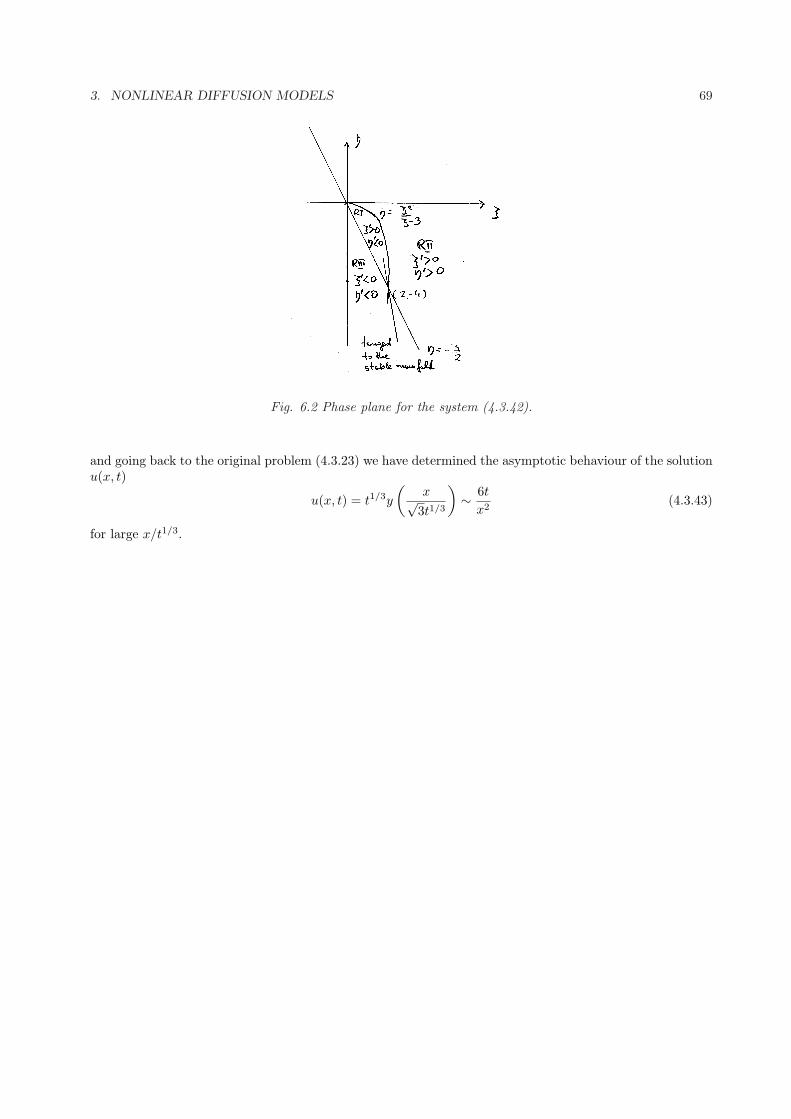
3. NONLINEAR DIFFUSION MODELS 69
Fig. 6.2 Phase plane for the system (4.3.42).
and going back to the original problem (4.3.23) we have determined the asymptotic behaviour of the solutionu(x, t)
u(x, t) = t1/3y
(x√
3t1/3
)∼ 6t
x2(4.3.43)
for large x/t1/3.

70 CHAPTER 4. SIMILARITY METHODS FOR LINEAR AND NON-LINEAR DIFFUSION
Chapter 5
Travelling waves
1 Introduction
One of the cornerstones in the study of both linear and nonlinear PDEs is the wave propagation. A wave isa recognizable signal which is transferred from one part of the medium to another part with a recognizablespeed of propagation. Energy is often transferred as the wave propagates, but matter may not be. Wemention here a few areas where wave propagation is of fundamental importance.
Fluid mechanics (water waves, aerodynamics)
Acoustics (sound waves in air and liquids)
Elasticity (stress waves, earthquakes)
Electromagnetic theory (optics, electromagnetic waves)
Biology (epizootic waves)
Chemistry (combustion and detonation waves)
The simplest form of a mathematical wave is a function of the form
u(x, t) = f(x− ct). (5.1.1)
We adopt the convention that c > 0. We have already seen such a wave as a solution of the constantcoefficient transport equation
ut + cux = 0,
it can, however, appear in many other contexts.
At t = 0 the wave has the form f(x) which is the initial wave profile. Then f(x− ct) represents the profileat time t, that is just the initial profile translated to the right by ct spatial units. Thus the constant crepresents the speed of the wave and thus, evidently, (5.1.1) represents a wave travelling to the right withspeed c > 0. Similarly,
u(x, t) = f(x + ct)
represents a wave travelling to the right with speed c. These waves propagate undistorted along the linesx± ct = const.
One of the fundamental questions in the theory of nonlinear PDEs is whether a given PDE admit such atravelling wave as a solution. This question is generally asked without regard to initial conditions so thatthe wave is assumed to have existed for all times. However, boundary conditions of the form
u(−∞, t) = constant, u(+∞, t) = constant (5.1.2)
71
72 CHAPTER 5. TRAVELLING WAVES
are usually imposed. A wavefront type-solution to a PDE is a solution of the form u(x, t) = f(x± ct) subjectto the condition (5.1.2) of being constant at ±∞ (this constant are not necessarily the same); the function fis assumed to have the requisite degree of smoothness defined by the PDE. If u approaches the same constantat both ±∞, then the wavefront is called a pulse.
2 Basic examples
We have already seen that the transport equation with constant c admits the travelling wave solution and itis the only solution this equation can have. To illustrate the technique of looking for travelling wave solutionson a simple example first, let us consider the wave equation.
Example 2.1 Find travelling wave solutions to the wave equation
utt − a2uxx = 0.
According to definition, travelling wave solution is of the form u(x, t) = f(x − ct). Inserting this into theequation, we find
utt − a2uxx = c2f ′′ − a2f ′′ = f ′′ · (c2 − a2) = 0
so that either f(s) = A + Bs for some constants A, B or c = ±a and f arbitrary. In the first case we wouldhave
u(x, t) = A + B(x± ct)
but the boundary conditions (5.1.2) cannot be satisfied unless B = 0. Thus, the only travelling wave solutionin this case is constant. For the other case, we see that clearly for any twice differentiable function f suchthat
lims→±∞
= d±∞
the solutionu(x, t) = f(x± at)
is a travelling wave solution (a pulse if d+∞ = d−∞).
In general, it follows that any solution to the wave equation can be obtained as a superposition of twotravelling waves: one to the right and one to the left
u(x, t) = f(x− at) + g(x + at).
Not all equations admit travelling wave solutions, as demonstrated below.
Example 2.2 Consider the diffusion equation
ut = Duxx.
Substituting the travelling wave formula u(x, t) = f(x− ct), we obtain
−cf ′ −Df ′′ = 0
that has the general solutionf(s) = a + b exp
(−cs
D
).
It is clear that for f to be constant at both plus and minus infinity it is necessary that b = 0. Thus, thereare no nonconstant travelling wave solutions to the diffusion equation.
We have already seen that the non-viscid Burger’s equation
ut + uux = 0
does not admit a travelling wave solution: any profile will either smooth out or form a shock wave (which canbe considered as a generalized travelling wave - it is not continuous!). However, some amount of dissipationrepresented by a diffusion term allows to avoid shocks.
3. THE BURGER EQUATION 73
3 The Burger equation
Consider Burger’s equation with viscosity
ut + uux − νuxx = 0, ν > 0. (5.3.3)
The term uux will have a shocking up effect that will cause waves to break and the term νuxx is a diffusionlike term.
3.1 Travelling wave solutions
We attempt to find a travelling wave solution of (5.3.3) of the form
u(x, t) = f(x− ct).
Substituting this to (5.3.3) we obtain
−cf ′(s) + f(s)f ′(s)− νf ′′(s) = 0,
where s = x− ct. Noting that ff ′ = 12 (f2)′ we re-write the above as
−cf ′ +12(f2)′ − νf ′′ = 0,
hence we can integrate getting
−cf +12f2 − νf ′ = B
where B is a constant of integration. Hence
df
ds=
12ν
(f2 − 2cf − 2B
). (5.3.4)
Let us consider the case when the quadratic polynomial above factorizes into real linear factors, that is(f2 − 2cf − 2B
)= (f − f1)(f − f2)
wheref1 = c−
√c2 + 2B, f2 = c +
√c2 + 2B. (5.3.5)
This requires c2 > 2B and yields, in particular, f2 > f1. Eq. (5.3.4) can be easily solved by separatingvariables. First note that f1 and f2 are the only equilibrium points and (f − f1)(f − f2) < 0 for f1 < f < f2
so that any solution starting between f1 and f2 will stay there tending to f1 as s → +∞ and to f2 ass → −∞. Any solution starting above f2 will tend to ∞ as s → +∞ and any one starting below f1 will tendto −∞ as s → −∞. Thus, the only non constant travelling wave solutions are possible for f1 < f < f2. Forsuch f integration if (4.3.26) yields
s− s0
2ν=
∫df
(f − f1)(f − f2)= − 1
f2 − f1
∫ (1
f − f1+
1f2 − f
)df
=1
f2 − f1ln
f2 − f
f − f1.
Solving for f yields
f(s) =f2 + f1e
K(s−s0)
1 + eK(s−s0), (5.3.6)
where K = 12ν (f2 − f1) > 0. We see that for large positive s f(s) ∼ f1 whereas for negative values of s we
obtain asymptotically f(s) ∼ f2. It is clear that the initial value s0 is not essential so that we shall suppressit in the sequel. The derivative of f is
f ′(s) = KeKs(f1 − f2)(1 + eKs)2
< 0.

74 CHAPTER 5. TRAVELLING WAVES
It is easy to see that for large |s| the derivative f(s) is close to zero so that f is almost flat. Moreover, thelarger ν (so that the smaller K), the more flat is f as the derivative is closer to zero. Hence, for small ν weobtain a very steep wave front that is consistent with the fact for ν = 0 we obtain inviscid Burger’s equationthat admits only discontinuous travelling waves.
The formula for travelling wave solution to (5.3.3) is then
u(x, t) =f2 + f1e
K(x−ct)
1 + eK(x−ct), (5.3.7)
where the speed of the wave is determined from (5.3.5) as
c =12(f1 + f2).
Graphically the travelling wave solution is the profile f moving to the right at speed c. This solution, becauseit resembles the actual profile of a shock wave, is called the shock structure solution; it joints the asymptoticstates f1 and f2. Without the term νuxx the solutions of (5.3.3) would shock up and tend to break. Thepresence of the diffusion term prevents this breaking effect by countering the nonlinearity. The result iscompetition and balance between the nonlinear term uux and the diffusion term −νuxx, much the same asoccurs in a real shock wave in the narrow region where the gradient is steep. In this context the −νuxx termcould be interpreted as a viscosity term.
3.2 The Cole-Hopf transformation and analytic solution to the Burgers equa-tion
Let us consider the simplified version of the Burgers equation
ut + uux − uxx = 0. (5.3.8)
It can be proved that the Burgers equation is equivalent to the linear diffusion equation. First we introducea new function by
u = wx.
Then (5.3.8) takes the form
wtx + wxwxx − wxxx = wtx +12(wx)2x − wxxx0
which can be integrated with respect to x to give
wt +12w2
x − wxx = c(t)
where x(t) is a function of time t. Next we introduce a new function v by the formula
w = −2 ln v.
Differentiation gives
wt = −2vt
v, wx = −2
vx
v, wxx = −2
vxx
v+ 2
v2x
v2.
Hence
wt +12w2
x − wxx = −2vt
v+ 2
v2x
v2+ 2
vxx
v− 2
v2x
v2= −2
vt
v+ 2
vxx
v= c(t)
which is the diffusion equation (with a growth/decay term).
vt − vxx = −2c(t)v.
3. THE BURGER EQUATION 75
If we denote C(t) =∫
c(t)dt then, using the integrating factor, we can write the above as the standarddiffusion equation
(veC(t))t − (veC(t))xx = 0.
Summarizing, if we can find a solution V (t, x) of the diffusion equation, then
u(x, t) = −2∂
∂xln
(v(x, t)eC(t)
)= −2
vx(x, t)v(x, t)
(5.3.9)
is a solution to the Burgers equation. We see, that the arbitrary function c(t) does not enter into the solutionu and thus we can focus on solving just
vt − vxx = 0.
So, any nonzero solution of the diffusion equation generates a unique solution of the Burgers equation.Conversely, if u is a solution to the Burgers equation, then the formula (5.3.9) determines v according to
v(x, t) = φ(t)e− 1
2
x∫0
u(s,t)ds
where φ is an arbitrary function of t. Differentiating, we obtain
vt(x, t) = φ′(t)e− 1
2
x∫0
u(s,t)ds− 1
2φ(t)
x∫
0
ut(s, t)dse−
x∫0
u(s,t)ds=
φ′(t)φ(t)
v(x, t)− 12v(x, t)
x∫
0
ut(s, t)ds
and, similarly,
vx = −12uv, vxx = −1
2uxv +
14u2v.
Consequently,
vt − vxx =12
φ′
φv − 1
2v
x∫
0
ut(s, t)ds− ux +12u2
where the expression in brackets is the integral with respect to x of the left hand side of (5.3.8), which isan arbitrary function of t. Hence, any solution to the Burgers equation generates a solution to the diffusionequation
vt − vxx = φ(t)v
for some function φ(t).
As our main interest is finding the solution to the Burgers equation, we write down the analytical formulafor the solution to the initial value problem
ut + uux − uxx = 0, u(x, 0) =u (x). (5.3.10)
Using (5.3.9), the initial condition (5.3.10) on u can be obtained from the initial condition on v given by
v (x) = e
− 12
x∫0
u(s)ds
The solution of the initial value problem for the diffusion equation is given by (4.2.16)
v(x, t) =1
2√
πt
∞∫
−∞e−
(x−ξ)2
4tv (ξ)dξ.
Therefore
vx(x, t) = − 12√
πt
∞∫
−∞
(x− ξ)2t
e−(x−ξ)2
4tv (ξ)dξ
76 CHAPTER 5. TRAVELLING WAVES
and
u(x, t) = −2vx(x, t)v(x, t)
= −
∞∫−∞
(x−ξ)t e−
(x−ξ)2
4tv (ξ)dξ
∞∫−∞
e−(x−ξ)2
4tv (ξ)dξ
or, introducing the kernel
G(x, ξ, t) = −12
ξ∫
0
u (s)ds− (x− ξ)2
4t
we obtain the formula explicitly involvingu as
u(x, t) = −
∞∫−∞
(x−ξ)t eG(x,ξ,t)dξ
∞∫−∞
eG(x,ξ,t)dξ
.
Remark 3.1 The considerations above have been done for a spacial case of the Burgers equation with ν = 1.If we have the general form of the equation
ut + auux = νuxx
then the substitution u(x, t) = νa−1U(x, νt) gives the simplified equation
Ut + UUx = Uxx.
Example 3.1 Find the solution to the following initial value problem
ut + uux = 2uxx, u(x, 0) = 2x.
Introducing a new unknown function u(x, t) = 2U(x, 2t) we see that ut = 4Uτ , ux = 2Ux, uxx = 2Uxx andthus have
0 = ut + uux = 2uxx = 4Uτ + 4UUx − 4Uxx
so that U satisfies the simplified Burgers equation with the initial condition U(x, 0) = x. We can then applythe transformation
U = −2Vx
V
to get the diffusion equationVt − Vxx = 0
subject to the initial conditionx
2= −2
Vx(x, 0)V (x, 0)
that isV (x, 0) = e−
14 x2
.
To solve the diffusion equation with this initial condition we can use several methods. We present the solutionby matching and by using the integral formula (4.2.16).
Method 1.We recognize that V (x, 0) has the form similar to the fundamental solution of the diffusion equation (4.2.11)
S(x, t) =1√4πt
e−x24t .
4. THE KORTEWEG-DE VRIES EQUATION AND SOLITONS 77
Since a solution of the diffusion equation multiplied by a constant is again a solution, we look for time t andconstant c such that
cS(x, t) = e−14 x2
,
which gives t = 1 and c = 2√
π. Thus 2√
πS(x, t) takes the value V (x, 0) at t = 1. Since the diffusionequation is invariant with respect to the shift of time, we obtain that
V (x, t) = 2√
πS(x, t + 1) =e−
x24(t+1)
√t + 1
is the sought solution. Consequently
U(x, t) = −2Vx
V=
x
t + 1and
u(x, t) = 2U(x, 2t) =2x
2t + 1.
Method 2.We have
V (x, t) =1
2√
πt
∞∫
−∞e−
(x−y)2
4t e−y2
4 dy.
Completing the quare in the exponent we get
x2 − 2xy + y2
4t+
y2
4=
x2 − 2xy + y2 + ty2
4t=
(x− y(1 + t))2
4t(1 + t)+
x2
4(1 + t)
hence
V (x, t) =e−
x24(t+1)
2√
πt
∞∫
−∞e−
(x−y(1+t))2
4t(1+t) dy.
Introducing the change of variable z = (x− y(1 + t))/2√
t(1 + t), so that dy = −2√
tdz/√
1 + t, we obtain
V (x, t) =e−
x24(t+1)
√π(1 + t)
∞∫
−∞e−z2
dz =e−
x24(t+1)
√(1 + t)
.
The last step follows as before.
4 The Korteweg-de Vries equation and solitons
The last example related to travelling waves is concerned with the so called solitons that appear in solutions ofnumerous important partial differential equations. The simples equation producing solitons is the Korteweg-deVries equation that governs long waves in shallow water. Find travelling wave solutions of the KdVequation
ut + uux + kuxxx = 0, (5.4.11)
where k > 0 is a constant. As before, we are looking for a solution of the form
u(x, t) = f(s), s = x− st,
where the waveform f and the wave speed c are to be determined. Substituting f into (5.4.11) we get
−cf ′ +12(f2)′ + kf ′′′ = 0,
78 CHAPTER 5. TRAVELLING WAVES
integration of which gives
−cf +12f2 + kf ′′ = a
for some constant a. This is a second order equation that does not contain the independent variable, hencewe can use substitution f ′ = F (f). Hence, f ′′s = F ′ff ′s = F ′fF and we can write
−cf +12f2 + kF ′fF = −cf +
12f2 +
k
2(F 2
f )′ = a.
Integrating, we get
F 2 =1k
(cf2 − 1
3f3 + 2af + 2b
)
where b is a constant. Thus,
f ′ = ±√
13k
(−f3 + 3cf2 + 6af + 6b)1/2
. (5.4.12)
To fix attention we shall take the ”+” sign. Denote by φ(f) the cubic polynomial on the right-hand side.We have the following possibilities:
(i) φ has one real root α;
(ii) φ has three distinct real roots γ < β < α;
(iii) φ has three real roots satisfying γ = β < α;
(iv) φ has three real roots satisfying γ < β = α;
(v) φ has a triple root γ.
Since we are looking for travelling wave solutions that should be bounded at ±∞ and nonnegative, we canrule out most of the cases by qualitative analysis describedNote first that the right-hand side of (5.4.12) isdefined only where φ(f) > 0. Then, in the case (i), α is a unique equilibrium point, φ > 0 only for f < αand hence any solution converges to α as t → ∞ and diverges to +∞ as t → −∞. Similar argument rulesout case (v).
If we have three distinct roots, then by the same argument, the only bounded solutions can exist in the cases(iii) and (ii) (in the case (iv) the bounded solutions could only appear where φ < 0. ) The case (ii) leadsto the so-called cnoidal waves expressible through special functions called cn-functions and hence the name.We shall concentrate on case (iii) so that
φ(f) = −f3 + 3cf2 + 6af + 6b = (γ − f)2(β − f)
and, since f > γ √φ(f) = (f − γ)
√α− f.
Thus, the differential equation (5.4.12) can be written
s√3k
=∫
df
(f − γ)√
α− f. (5.4.13)
To integrate, we first denote v = f − γ and B = α− γ (with 0 < v < b), getting
s√3k
=∫
dv
v√
B − v.
Next, we substitute w =√
B − v, hence v = B − w2 and dw = −ds/2√
B − v so that the above will betransformed to
s√3k
= 2∫
dw
w2 −B.

5. THE FISHER EQUATION 79
This integral can be evaluated by partial fractions, so that, using 0 < w <√
B, we get
s√3k
=1√B
∫ (dw
w −√B− dw
w +√
B
)dw =
1√B
ln√
B − w√B + w
.
Solving with respect to w we obtain √B − w√B + w
= exp s
√B
3k
and thus
w =√
B1− exp s
√B3k
1 + exp s√
B3k
= −√
Bsinh s
√B
12k
cosh s√
B12k
.
Returning to the original variables w2 = B − v = α − γ − f + γ = α − f and using the hyperbolic identitycosh2 θ − sinh2 θ = 1, we get
f(s) = α− w2(s) = α− (α− γ)sinh2 s
√α−γ12k
cosh2 s√
α−γ12k
= γ + (α− γ)sech2
(s
√α− γ
12k
)
Clearly, f(s) → γ as s → ±∞ so that the travelling wave here is a pulse. It is instructive to write the rootsα and γ in terms of the original parameters. To identify them we observe
φ(f) = −f3 + 3cf2 + 6af + 6b = (γ − f)2(β − f)= −f3 + f2(α + 2γ) + f(−γ2 − 2αγ) + γ2α.
Thus, the wave speed is given by
c =α + 2γ
3=
α− γ
3+ γ.
Since γ is just the level of the wave at ±∞, by moving the coordinate system we can make it equal to zero.In this case we can write the travelling wave solution to the KdV equation as
u(x, t) = 3csech2
(√√c
4k(x− ct)
)(5.4.14)
It is important to note that the velocity of this wave is proportional to its amplitude which makes it differentfrom linear waves governed by, say the wave equation, where the wave velocity is the property of the mediumrather than of the wave itself.
5 The Fisher equation
Many natural processes involve mechanisms of both diffusion and reaction, and such problems are oftenmodelled by so-called reaction-diffusion equations of the form
ut −Duxx = f(u), (5.5.15)
where f is a given, usually nonlinear function of u. We introduced earlier the Fisher equation
ut −Duxx = ru(1− u
K
)(5.5.16)
80 CHAPTER 5. TRAVELLING WAVES
to model the diffusion of a species (e.g. insect population) when the reaction (or, at this instance) growthterm is given by the logistic law. Here D is the diffusion constant, and r and K are the growth rate andcarrying capacity, respectively.
We shall examine the Fisher equation and, in particular, we shall address the question of existence of atravelling wave solution.
Let us consider the Fisher equation in dimensionless form
ut − uxx = u(1− u) (5.5.17)
and, as before, we shall look for solutions of the form
u(x, t) = U(s), s = x− ct, (5.5.18)
where c is a positive constant and U has the property that it approaches constant values at s → ±∞. Thefunction U to be determined should be twice differentiable. The wave speed c is a priori unknown and mustbe determined as a part of the solution of the problem. Substituting (5.5.18) into (5.5.17) yields a secondorder ordinary differential equation for U :
−cU ′ − U ′′ = U(1− U). (5.5.19)
Contrary to the previous cases, this equation cannot be solved in a closed form and the best approach toanalyze it is to perform the phase plane analysis. In a standard way we write (5.5.19) as a simultaneoussystem of first order equations by defining V = U ′. In this way we obtain
U ′ = V,
V ′ = −cV − U(1− U). (5.5.20)
We find equilibrium points of this system solving
0 = V,
0 = −cV − U(1− U),
which gives two: (0, 0) and (0, 1). The Jacobi matrix of the system is
J(U, V ) =(
0 12U − 1 −c
)
so that
J(0, 0) =(
0 1−1 −c
)
with eigenvalues
λ0,0± =
−c±√c2 − 42
and
J(1, 0) =(
0 11 −c
)
with eigenvalues
λ1,0± =
−c±√c2 + 42
.
It is easily seen that for any c, λ1,0± are real and of opposite sign and therefore (1, 0) is a saddle. On the
other hand, λ0,0± are both real and negative if c ≥ 2 and in this case (0, 0) is a stable node (for the linearized
system), and are complex with negative real part if 0 < c < 2 in which case (0, 0) is a stable focus.
Since the wave profile U(s) must have finite limits as s → ±∞ and since we know that the only limit pointsof solutions of autonomous systems are equilibrium points, search for travelling wave solutions of (5.5.19) is
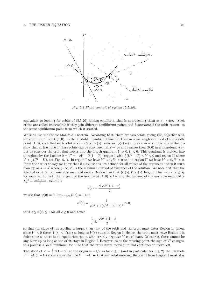
5. THE FISHER EQUATION 81
Fig. 5.1 Phase portrait of system (5.5.20).
equivalent to looking for orbits of (5.5.20) joining equilibria, that is approaching them as s → ±∞. Suchorbits are called heteroclinic if they join different equilibrium points and homoclinic if the orbit returns tothe same equilibrium point from which it started.
We shall use the Stable Manifold Theorem. According to it, there are two orbits giving rise, together withthe equilibrium point (1, 0), to the unstable manifold defined at least in some neighbourhood of the saddlepoint (1, 0), such that each orbit φ(s) = (U(s), V (s)) satisfies: φ(s) to(1, 0) as s → −∞. Our aim is then toshow that at least one of these orbits can be continued till s →∞ and reaches then (0, 0) in a monotonic way.Let us consider the orbit that moves into the fourth quadrant U > 0, V < 0. This quadrant is divided intoto regions by the isocline 0 = V ′ = −cV − U(1− U): region I with 1
c (U2 − U) < V < 0 and region II whereV < 1
c (U2 − U), see Fig. 5. 1. In region I we have V ′ < 0, U ′ < 0 and in region II we have V ′ > 0, U ′ < 0.From the earlier theory we know that if a solution is not defined for all values of the argument s then it mustblow up as s → s′ where (−∞, s′) is the maximal interval of existence of the solution. We note first that theselected orbit on our unstable manifold enters Region I so that (U(s), V (s)) ∈ Region I for −∞ < s ≤ s0
for some s0. In fact, the tangent of the isocline at (1, 0) is 1/c and the tangent of the unstable manifold isλ1,0
+ =√
c2+4−c2 . Denoting
ψ(c) =c(√
c2 + 4− c)2
we see that ψ(0) = 0, limc→+∞ ψ(s) = 1 and
ψ′(c) =4√
c2 + 4(√
c2 + 4 + c)2> 0,
thus 0 ≤ ψ(c) ≤ 1 for all c ≥ 0 and hence
1c≥√
c2 + 4− c
2,
so that the slope of the isocline is larger than that of the orbit and the orbit must enter Region 1. Then,since V ′ < 0 there, V (s) < V (s0) as long as V (s) stays in Region I. Hence, the orbit must leave Region I infinite time as there is no equilibrium point with strictly negative V coordinate. Of course, there cannot beany blow up as long as the orbit stays in Region I. However, as at the crossing point the sign of V ′ changes,this point is a local minimum for V so that the orbit starts moving up and continues to move left.
The slope of V = 1cU(1 − U) at the origin is −1/c so for c ≥ 1 (and in particular for c ≥ 2) the parabola
V = 1cU(1− U) stays above the line V = −U so that any orbit entering Region II from Region I must stay
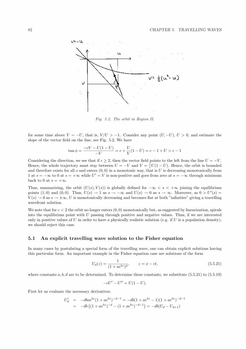
82 CHAPTER 5. TRAVELLING WAVES
Fig. 5.2. The orbit in Region II.
for some time above V = −U , that is, V/U > −1. Consider any point (U,−U), U > 0, and estimate theslope of the vector field on the line, see Fig. 5.2, We have
tan φ =−cV − U(1− U)
−V= c +
U
V(1− U) = c− 1 + U > c− 1
Considering the direction, we see that if c ≥ 2, then the vector field points to the left from the line U = −V .Hence, the whole trajectory must stay between U = −V and V = 1
cU(1− U). Hence, the orbit is boundedand therefore exists for all s and enters (0, 0) in a monotonic way, that is U is decreasing monotonically from1 at s = −∞ to 0 at s = +∞ while U ′ = V is non-positive and goes from zero at s = −∞ through minimumback to 0 at s = +∞.
Thus, summarizing, the orbit (U(s), V (s)) is globally defined for −∞ < s < +∞ joining the equilibriumpoints (1, 0) and (0, 0). Thus, U(s) → 1 as s → −∞ and U(s) → 0 as s → ∞. Moreover, as 0 > U ′(s) =V (s) → 0 as s → ±∞, U is monotonically decreasing and becomes flat at both ”infinities” giving a travellingwavefront solution.
We note that for c < 2 the orbit no longer enters (0, 0) monotonically but, as suggested by linearization, spiralsinto the equilibrium point with U passing through positive and negative values. Thus, if we are interestedonly in positive values of U in order to have a physically realistic solution (e.g. if U is a population density),we should reject this case.
5.1 An explicit travelling wave solution to the Fisher equation
In many cases by postulating a special form of the travelling wave, one can obtain explicit solutions havingthis particular form. An important example in the Fisher equation case are solutions of the form
Ud(z) =1
(1 + aebz)d, z = x− ct, (5.5.21)
where constants a, b, d are to be determined. To determine these constants, we substitute (5.5.21) to (5.5.19)
−cU ′ − U ′′ = U(1− U).
First let us evaluate the necessary derivatives.
U ′d = −dbaebz(1 + aebz)−d−1 = −db(1 + aebz − 1)(1 + aebz)−d−1
= −db((1 + aebz)−d − (1 + aebz)−d−1
)= −db(Ud − Ud+1)
6. THE NAGUMO EQUATION 83
and similarlyU ′′
d = db2(dUd − (2d + 1)Ud+1 + (d + 1)Ud+2).
On the other handU(1− U) = Ud − U2d
so thatcdb(Ud − Ud+1)− db2(dUd − (2d + 1)Ud+1 + (d + 1)Ud+2) = Ud − U2d
Since Ud = (U1)d and y = U1(z) is a one-to-one mapping of (−∞,∞) onto (0, 1), the above equation isequivalent to the polynomial equation
y2d − d(d + 1)b2yd+2 + (d(2d + 1)b2 − cdb)yd+1 + (cdb− (db)2 − 1)yd = 0, y ∈ (0, 1).
Since a polynomial is identically equal zero on an open interval if and only if all coefficients are 0, we obtainthree possible cases: 2d = d+2, 2d = d+1 or 2d = d. The last one gives d = 0 and thus a constant solution.The second results in d = 1 and thus d(d + 1)b = 0, yielding b = 0 and again we obtain a constant solution.Let us consider the first case. Then d = 2 and thus, equating to zero coefficients of like powers
1− 6b2 = 0,
2b(5b− c) = 0,
2cb− 4b2 − 1 = 0,
we immediately obtain b = ±1/√
6, c = ±5/√
6 and it is easy to see that the last equation is automaticallysatisfied. Hence, we obtained a family of travelling wave of the Fisher equation
u(x, t) =1
(1 + ae±√
6x∓5t6 )2
.
The arbitrary parameter a > 0 determines how steep is the wave.
6 The Nagumo equation
The Fisher equation describes spreading of a population which locally reproduces according to the logisticlaw. More sophisticated reproduction laws include the so-called Allee effect describing the situation in whichsmall populations die out. Mathematically the Allee effect is represented by a term with three equilibria0 < L < K, where K is the carrying capacity of the environment and L is the threshold below which thepopulation perishes. In the normalized case we consider the equation
ut = uxx + u(u− a)(1− u) (5.6.22)
where 0 < a < 1. u is normalized density of the population and we assume that 0 < u < 1. This equation iscalled the Nagumo equation. We look for some explicit travelling wave solutions to this equation. As before,we introduce u(x, t) = U(x− ct), 0 < U < 1, which converts (5.6.22) to
−cU ′z = U ′′
zz + U(U − a)(1− U), z = x− ct.
As long as U ′z 6= 0, we can reduce this equation to the first order equation
(Ψ2)′U = −2cΨ− 2U3 − 2(1 + a)U2 + 2aU
where Ψ(U) = U ′z and U ′′
zz = Ψ′UΨ. If we try to find polynomial (in U) solutions to the above equation, thenwe see that the lowest order polynomial which could provide a solution is quadratic. Consider thus
Ψ(U) = γ + βU + αU2.

84 CHAPTER 5. TRAVELLING WAVES
Then(Ψ2(U))′ = 2γβ + 2(2γα + β2)U + 6αβU3 + 4α2U3
and, comparing like powers of U , we obtain
2γβ = −2cγ,
2(2γα + β2) = −2cβ + 2a,
6αβ = −2cα− 2(1 + a),4α2 = 2.
From the last equation α = ±1/√
2. We shall work with the plus sign to keep the notation simpler. Thus
γ(β + c) = 0, (5.6.23)√2γ + β2 = −cβ + a, (5.6.24)
3β = −c−√
2(1 + a). (5.6.25)
From the last equation c = −3β −√2(1 + a) and the first equation becomes
γ(2β +√
2(1 + a)) = 0.
Now, we have to distinguish two cases.Case 1. γ = 0.In this case the second equation gives
4β2 + 2√
2(1 + a) + 2a = 0
and we obtain solutionsβ1,2 = − a√
a,− 1√
2.
In the first caseΨ(U) =
1√2U(U − a)
so that Ψ(U) = U ′z becomes 0 for U = a. It means that there is a possibility that the transformation reducing
the second order equation to the first order maybe not invertible at some point and thus we discard thissolution. The second case gives
Ψ(U) =1√2U(U − 1)
and Ψ(U) 6= 0 in the range where U is allowed to change. So, we shall use this solution with
c =√
2(
12− a
). (5.6.26)
Case 2. γ 6= 0.In this case
−c = β = − 1√2(1 + a)
and, from the second equation in (5.6.25), γ = a/√
2. Thus
Ψ(U) =a√2− 1√
2(1 + a)U +
1√2U2 =
1√2(a− U)(1− U)
and, again, we see that U ′ can vanish for some U ∈ (0, 1). Hence, again we rule this case out.
Thus, we are left with the equation
U ′ =1√2U(U − 1).
6. THE NAGUMO EQUATION 85
This is a separable equation which we solve by partial fractions. For U ∈ (0, 1)
K +z√2
=∫
dU
U+
∫dU
1− U= ln
U
1− U
for some constant K, that is,
U(z) =Ke
z√2
1 + Kez√2
and we obtain a travelling wave in the form
u(x, t) =Ke
x−ct√2
1 + Kex−ct√
2
.