Introduction to Neural Networks U. Minn. Psy 5038 Daniel ...vision.psych.umn.edu/users/kersten/kersten-lab/courses/Psy5038WF… · Introduction to Neural Networks U. Minn. Psy 5038

Introduction to Neural NetworksU. Minn. Psy 5038Daniel KerstenBelief Propagation

Initialize

‡ Read in Statistical Add-in packages:

In[1]:= Off@General::spell1D;Needs@"ErrorBarPlots`"D

Last time

Generative modeling: Multivariate gaussian, mixtures

‡ Drawing samples

‡ Mixtures of gaussians

‡ Will use mixture distributions in the next lecture on EM application to segmentation

Introduction to Optimal inference and taskIntroduction to Bayesian learning

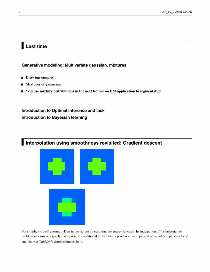
Interpolation using smoothness revisited: Gradient descent

For simplicity, we'll assume 1-D as in the lecture on sculpting the energy function. In anticipation of formulating the problem in terms of a graph that represents conditional probability dependence, we represent observable depth cues by y*, and the true ("hidden") depth estimates by y.

2 Lect_24_BeliefProp.nb

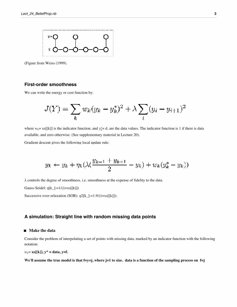
(Figure from Weiss (1999).

First-order smoothnessWe can write the energy or cost function by:

where wk= xs[[k]] is the indicator function, and yk*= d, are the data values. The indicator function is 1 if there is data available, and zero otherwise. (See supplementary material in Lecture 20).

Gradient descent gives the following local update rule:

l controls the degree of smoothness, i.e. smoothness at the expense of fidelity to the data.

Gauss-Seidel: h[k_]:=1/(l+xs[[k]])

Successive over-relaxation (SOR): h2[k_]:=1.9/(l+xs[[k]]);

A simulation: Straight line with random missing data points

‡ Make the data

Consider the problem of interpolating a set of points with missing data, marked by an indicator function with the following notation:

wk= xs[[k]], y* = data, y=f.

We'll assume the true model is that f=y=j, where j=1 to size. data is a function of the sampling process on f=j

Lect_24_BeliefProp.nb 3

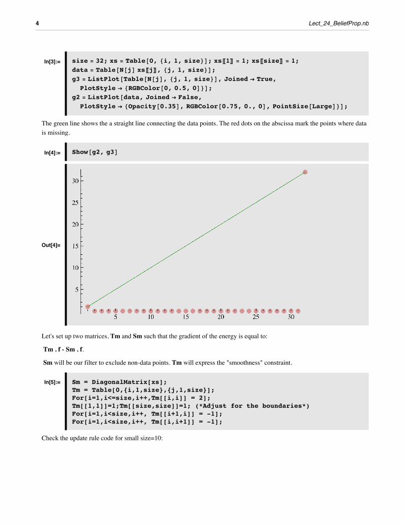
In[3]:= size = 32; xs = Table@0, 8i, 1, size<D; xsP1T = 1; xsPsizeT = 1;data = Table@N@jD xsPjT, 8j, 1, size<D;g3 = ListPlot@Table@N@jD, 8j, 1, size<D, Joined Ø True,PlotStyle Ø 8RGBColor@0, 0.5, 0D<D;

g2 = ListPlot@data, Joined Ø False,PlotStyle Ø [email protected], [email protected], 0., 0D, PointSize@LargeD<D;

The green line shows the a straight line connecting the data points. The red dots on the abscissa mark the points where data is missing.

In[4]:= Show@g2, g3D

Out[4]=

Let's set up two matrices, Tm and Sm such that the gradient of the energy is equal to:

Tm . f - Sm . f.

Sm will be our filter to exclude non-data points. Tm will express the "smoothness" constraint.

In[5]:= Sm = DiagonalMatrix[xs];Tm = Table[0,{i,1,size},{j,1,size}];For[i=1,i<=size,i++,Tm[[i,i]] = 2];Tm[[1,1]]=1;Tm[[size,size]]=1; (*Adjust for the boundaries*)For[i=1,i<size,i++, Tm[[i+1,i]] = -1];For[i=1,i<size,i++, Tm[[i,i+1]] = -1];

Check the update rule code for small size=10:


In[11]:= Clear@f, d, lDHl * Tm.Array@f, sizeD - Sm.HHArray@d, sizeDL - Array@f, sizeDLL êê

MatrixForm ;

‡ Run gradient descent

In[13]:= Clear[Tf,f1];dt = 1; l=2;Tf[f1_] := f1 - dt*(1/(l+xs))*(Tm.f1 - l*Sm.(data-f1));

We will initialize the state vector to zero, and then run the network for iter iterations:

In[16]:= iter=256;f = Table[0,{i,1,size}];result = Nest[Tf,f,iter];

Now plot the interpolated function.


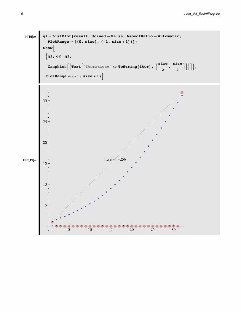
In[19]:= g1 = ListPlot@result, Joined Ø False, AspectRatio Ø Automatic,PlotRange Ø 880, size<, 8-1, size + 1<<D;

ShowB:g1, g2, g3,

GraphicsB:TextB"Iteration=" <> ToString@iterD, :size2

,size

2>F>F>,

PlotRange Ø 8-1, size + 1<F

Out[19]=


Try starting with f = random values between 0 and 40. Try various numbers of iterations.

Try different sampling functions xs[[i]].

Belief Propagation

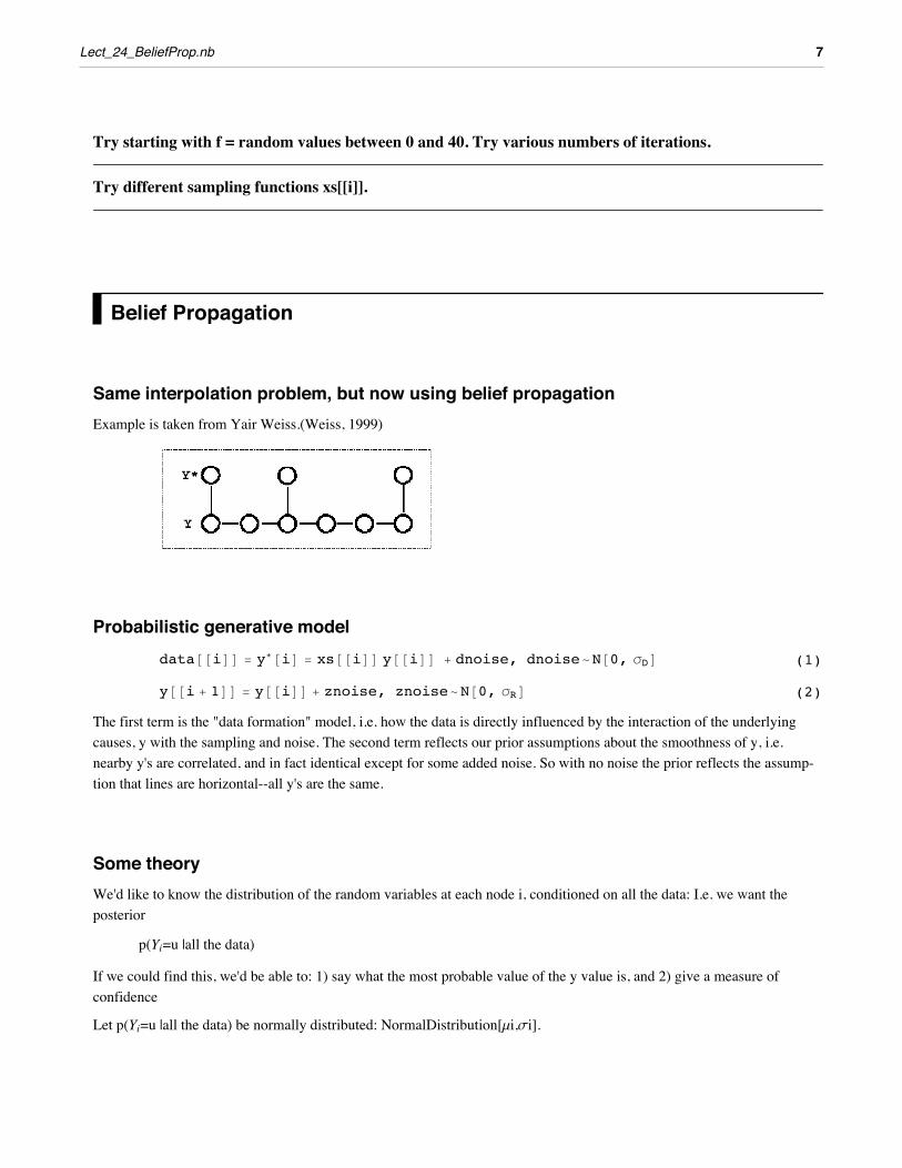
Same interpolation problem, but now using belief propagationExample is taken from Yair Weiss.(Weiss, 1999)

Probabilistic generative model(1)data@@iDD = y*@iD = xs@@iDD y@@iDD + dnoise, dnoise~N@0, sDD(2)y@@i + 1DD = y@@iDD + znoise, znoise~N@0, sRD

The first term is the "data formation" model, i.e. how the data is directly influenced by the interaction of the underlying causes, y with the sampling and noise. The second term reflects our prior assumptions about the smoothness of y, i.e. nearby y's are correlated, and in fact identical except for some added noise. So with no noise the prior reflects the assump-tion that lines are horizontal--all y's are the same.

Some theoryWe'd like to know the distribution of the random variables at each node i, conditioned on all the data: I.e. we want the posterior

p(Yi=u |all the data)

If we could find this, we'd be able to: 1) say what the most probable value of the y value is, and 2) give a measure of confidence

Let p(Yi=u |all the data) be normally distributed: NormalDistribution[mi,si].

Consider the ith unit. The posterior p(Yi=u|all the data) =


Consider the ith unit. The posterior p(Yi=u|all the data) =

(3)p(Yi=u|all the data) ∝ p(Yi=u|data before i) p(data at i| Yi=u) p(Yi=u|data after i)

Suppose that p(Yi=u | data before i) is also gaussian:

p(Yi=u|data before i) = a[u] ~ NormalDistribution[ma,sa]

and so is probability conditioned on the data after i:

p(Yi=u|data after i)= b[u] ~ NormalDistribution[mb,sb]

And the noise model for the data:

p(data at i| Yi=u) = L[u]~ NormalDistribution@yp, sDDyp=data[[i]]

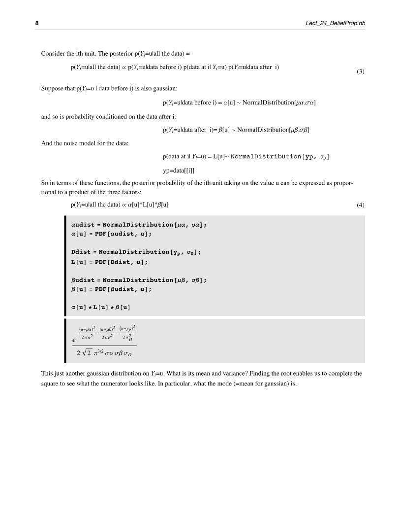
So in terms of these functions, the posterior probability of the ith unit taking on the value u can be expressed as propor-tional to a product of the three factors:

(4)p(Yi=u|all the data) ∝ a[u]*L[u]*b[u]

audist = NormalDistribution@ma, saD;a@uD = PDF@audist, uD;

Ddist = NormalDistribution@yp, sDD;L@uD = PDF@Ddist, uD;

budist = NormalDistribution@mb, sbD;b@uD = PDF@budist, uD;

a@uD * L@uD * b@uD

‰-Hu-maL22sa2

-Hu-mbL22sb2

-Iu-ypM22sD2

2 2 p3ê2 sasbsD

This just another gaussian distribution on Yi=u. What is its mean and variance? Finding the root enables us to complete the square to see what the numerator looks like. In particular, what the mode (=mean for gaussian) is.


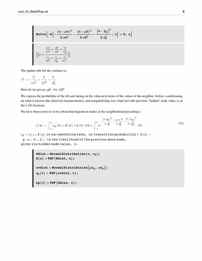
SolveB-DB- Hu - maL22 sa2

-Hu - mbL22 sb2

-Iu - ypM2

2 sD2

, uF ã 0, uF

::u Ø

ma

sa2+

mb

sb2+

yp

sD2

1sb2

+ 1sD2 + 1

sa2

>>

The update rule for the variance is:

s2 ->1

sa2+

1

sb2+

1

sD2

How do we get ma, mb , sa, sb?

We express the probability of the ith unit taking on the value u in terms of the values of the neighbor before, conditioning on what is known (the observed measurements), and marginalizing over what isn't (the previous "hidden" node value, v, at the i-1th location).

We have three terms to worry about that depend on nodes in the neighborhood preceding i:

(5)a@uD = ‡

-¶

¶

ap@vD * S@uD * L@vD „v ∝ ‡-¶

¶

‰-Iv-ypM2

2 sD2

-Hu-vL22 sR

2-Jv-mapN2

2 sap2

„v

ap = ai-1. S@uD is our smoothing term, or transition probability : S@uD =

p Hu » vL. L@D is the likelihood of the previous data node,given its hidden node value, v.

Rdist = NormalDistribution@v, sRD;S@uD = PDF@Rdist, uD;

avdist = NormalDistributionAmap, sapE;ap@vD = PDF@avdist, vD;

Lp@vD = PDF@Ddist, vD;


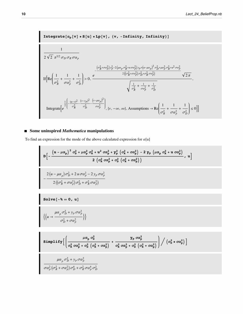
Integrate@ap@vD * S@uD * Lp@vD, 8v, -Infinity, Infinity<D

1

2 2 p3ê2 sD sR sap

IfBRe1

sR2+

1

sap2+

1

sD2

> 0,‰-JsR2 +sap2 N yp2-2 Jmap sR2 +usap2 N yp+Ju-mapN

2 sD2 +map

2 sR2 +u2 sap

2

2 JJsR2 +sap2 NsD2 +sR2 sap2 N 2 p

1sR2 + 1

sap2 + 1

sD2

,

IntegrateB‰12

-Hu-vL2sR2

-Iv-ypM2sD2

-Jv-mapN2

sap2

, 8v, -¶, ¶<, Assumptions Ø Re1

sR2+

1

sap2+

1

sD2

§ 0FF

‡ Some uninspired Mathematica manipulations

To find an expression for the mode of the above calculated expression for a[u]

DB-Iu - mapM2 sD

2 + map2 sR

2 + u2 sap2 + yp

2 IsR2 + sap2M - 2 yp Imap sR

2 + u sap2M

2 IsR2 sap2 + sD

2 IsR2 + sap2MM

, uF

-2 Iu - mapMsD

2 + 2 usap2 - 2 yp sap2

2 IIsR2 + sap

2 MsD2 + sR

2 sap2 M

Solve@-% ã 0, uD

::u Ømap sD

2 + yp sap2

sD2 + sap

2>>

SimplifyBmap sD

2

sR2 sap

2 + sD2 IsR2 + sap

2M+

yp sap2

sR2 sap

2 + sD2 IsR2 + sap

2Mì IsD2 * sap

2MF

map sD2 + yp sap2

sap2 IsR

2 + sap2 MsD

4 + sR2 sap

4 sD2


SimplifyB sD2

sR2 sap

2 + sD2 IsR2 + sap

2M+

sap2

sR2 sap

2 + sD2 IsR2 + sap

2Mì IsD2 * sap

2MF

sD2 + sap

2

sap2 IsR

2 + sap2 MsD

4 + sR2 sap

4 sD2

map sD2 + yp sap

2

sD2 sR

2 sap4 + sD

4 sap2 IsR2 + sap

2Mì

sD2 + sap

2

sD2 sR

2 sap4 + sD

4 sap2 IsR2 + sap

2M

map sD2 + yp sap2

sD2 + sap

2

So we now have rule that tells us how to update the a(u)=p(yi=u|data before i), in terms of the mean and variance parame-ters of the previous node:

ma map sD

2 + yp sap2

sD2 + sap

2=

map sD2

sap2 sD

2+

yp sap2

sap2 sD

2

sD2

sap2 sD

2+

sap2

sap2 sD

2

=

map

sap2

+yp

sD2

1

sap2

+ 1

sap2

The update rule for the variance is:

sa2 sR2 +

11

sD2

+ 1

sap2

A similar derivation gives us the rules for mb, sb2

mb

mba

sba2+ya

sD2

1

sba2+

1

saa2

sb2 sR2 +

11

sD2

+ 1

sba2

Where the subscript index p (for "previous", i.e. unit i-1) is replaced by a (for "after", i.e. unit i+1).

Recall that sometimes we have data and sometimes we don't. So replace:

(6)yp Ø xs@i - 1D data@i - 1D = wi-1 yi-1*

And similarly for ya.


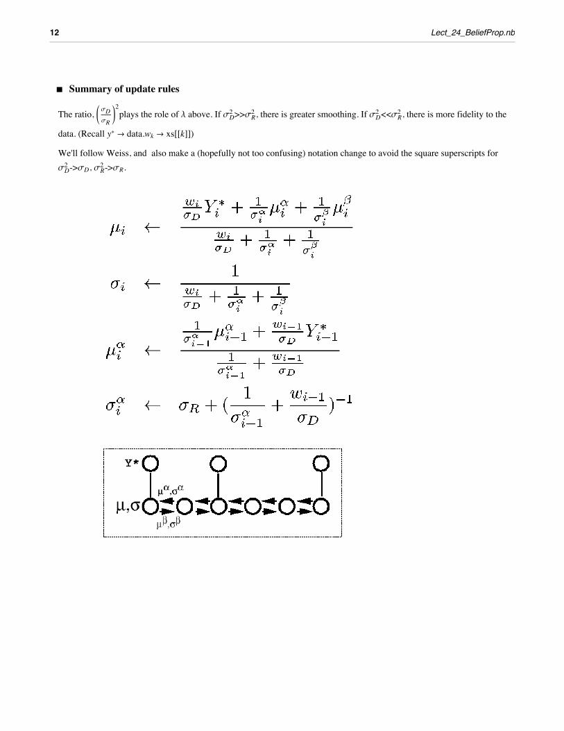
‡ Summary of update rules

The ratio, KsDsR

O2plays the role of l above. If sD2 >>sR

2 , there is greater smoothing. If sD2 <<sR

2 , there is more fidelity to the

data. (Recall y* Ø data.wk Ø xs@@kDD)We'll follow Weiss, and also make a (hopefully not too confusing) notation change to avoid the square superscripts for sD2 ->sD, sR

2 ->sR.


A simulation: Belief propagation for interpolation with missing data

‡ Initialization

In[37]:= size = 32;m0 = 1;ma = 1; sa = 100 000; H*large uncertainty *Lmb = 1; sb = 100 000;H*large*LsR = 4.0; sD = 1.0;– = Table@m0, 8i, 1, size<D;s = Table@sa, 8i, 1, size<D;–a = Table@m0, 8i, 1, size<D;sa = Table@sa, 8i, 1, size<D;–b = Table@m0, 8i, 1, size<D;sb = Table@sb, 8i, 1, size<D;iter = 0;i = 1;j = size;

The code below implements the above iterative equations, taking care near the boundaries. The plot shows the estimates of yi= µ, and the error bars show ±si.


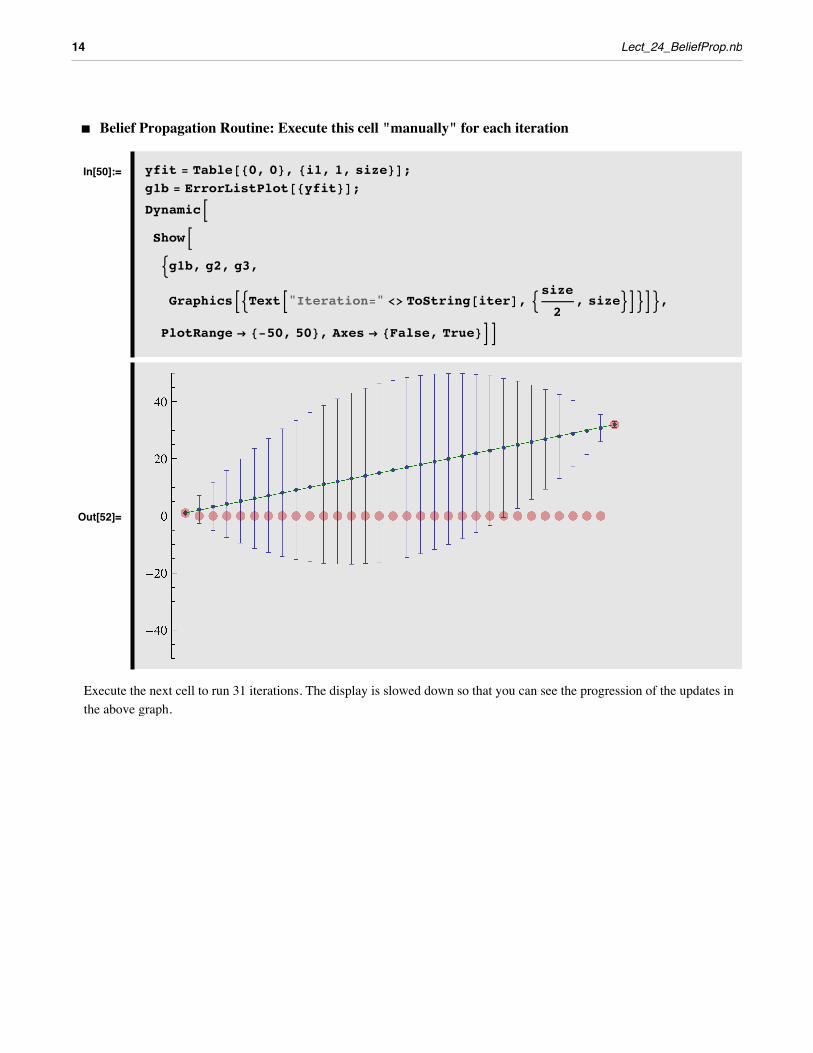
‡ Belief Propagation Routine: Execute this cell "manually" for each iteration

In[50]:= yfit = Table@80, 0<, 8i1, 1, size<D;g1b = ErrorListPlot@8yfit<D;DynamicBShowB:g1b, g2, g3,

GraphicsB:TextB"Iteration=" <> ToString@iterD, :size2

, size>F>F>,

PlotRange Ø 8-50, 50<, Axes Ø 8False, True<FF

Out[52]=

Execute the next cell to run 31 iterations. The display is slowed down so that you can see the progression of the updates in the above graph.


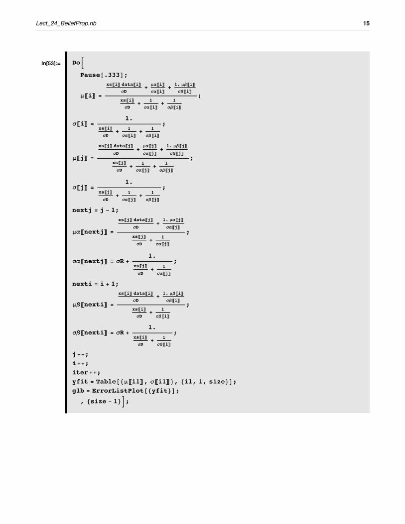
In[53]:= [email protected];

–PiT =

xsPiT dataPiTsD

+ –aPiTsaPiT + 1. –bPiT

sbPiTxsPiTsD

+ 1saPiT + 1

sbPiT

;

sPiT =1.

xsPiTsD

+ 1saPiT + 1

sbPiT

;

–PjT =

xsPjT dataPjTsD

+–aPjTsaPjT +

1. –bPjTsbPjT

xsPjTsD

+ 1saPjT + 1

sbPjT

;

sPjT =1.

xsPjTsD

+ 1saPjT + 1

sbPjT

;

nextj = j - 1;

–aPnextjT =

xsPjT dataPjTsD

+1. –aPjTsaPjT

xsPjTsD

+ 1saPjT

;

saPnextjT = sR +1.

xsPjTsD

+ 1saPjT

;

nexti = i + 1;

–bPnextiT =

xsPiT dataPiTsD

+ 1. –bPiTsbPiT

xsPiTsD

+ 1sbPiT

;

sbPnextiT = sR +1.

xsPiTsD

+ 1sbPiT

;

j--;i++;iter++;yfit = Table@8–Pi1T, sPi1T<, 8i1, 1, size<D;g1b = ErrorListPlot@8yfit<D;, 8size - 1<F;


Exercises

Run the descent algorithm using successive over-relaxation (SOR): h2[k_]:=1.9/(l+xs[[k]]). How does convergence compare with Gauss-Seidel?

Run Belief Propation using: sR=1.0; sD=4.0; How does fidelity to the data compare with the original case (sR=4.0; sD=1.0).

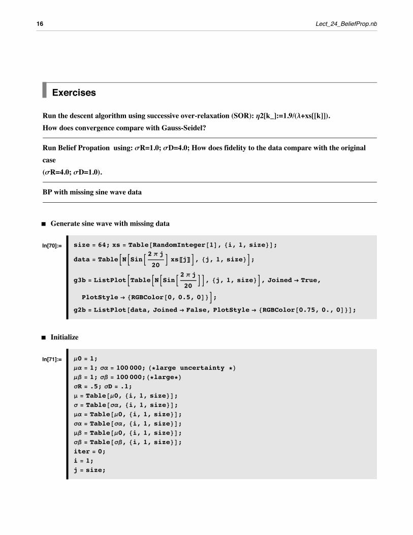
BP with missing sine wave data

‡ Generate sine wave with missing data

In[70]:= size = 64; xs = Table@RandomInteger@1D, 8i, 1, size<D;data = TableBNBSinB2 p j

20F xsPjTF, 8j, 1, size<F;

g3b = ListPlotBTableBNBSinB2 p j

20FF, 8j, 1, size<F, Joined Ø True,

PlotStyle Ø 8RGBColor@0, 0.5, 0D<F;g2b = ListPlot@data, Joined Ø False, PlotStyle Ø [email protected], 0., 0D<D;

‡ Initialize

In[71]:= m0 = 1;ma = 1; sa = 100 000; H*large uncertainty *Lmb = 1; sb = 100 000;H*large*LsR = .5; sD = .1;– = Table@m0, 8i, 1, size<D;s = Table@sa, 8i, 1, size<D;–a = Table@m0, 8i, 1, size<D;sa = Table@sa, 8i, 1, size<D;–b = Table@m0, 8i, 1, size<D;sb = Table@sb, 8i, 1, size<D;iter = 0;i = 1;j = size;


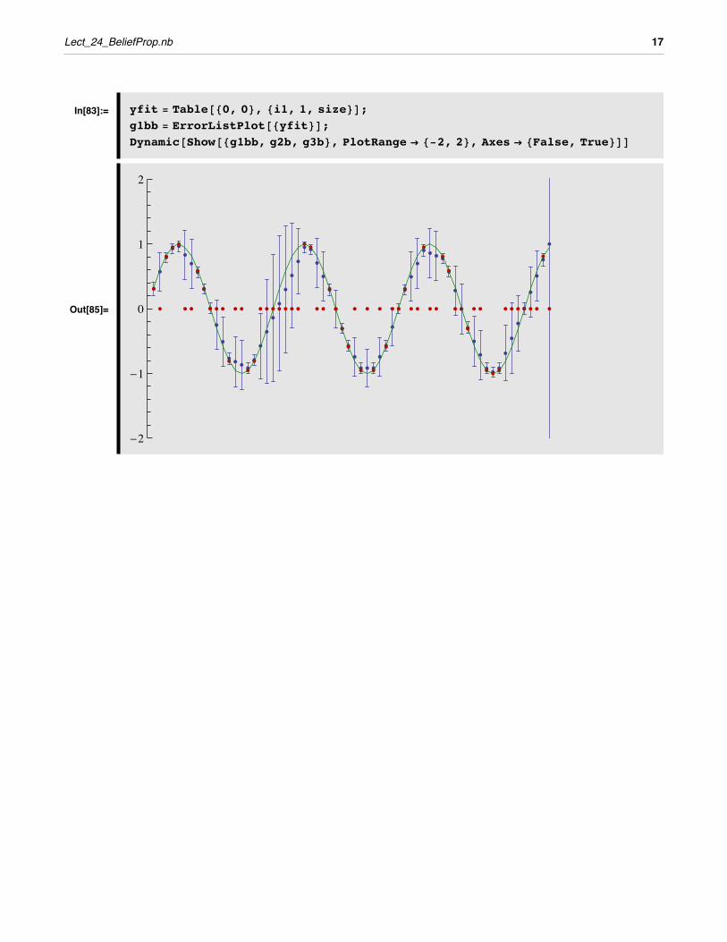
In[83]:= yfit = Table@80, 0<, 8i1, 1, size<D;g1bb = ErrorListPlot@8yfit<D;Dynamic@Show@8g1bb, g2b, g3b<, PlotRange Ø 8-2, 2<, Axes Ø 8False, True<DD

Out[85]=

-2

-1

0

1

2


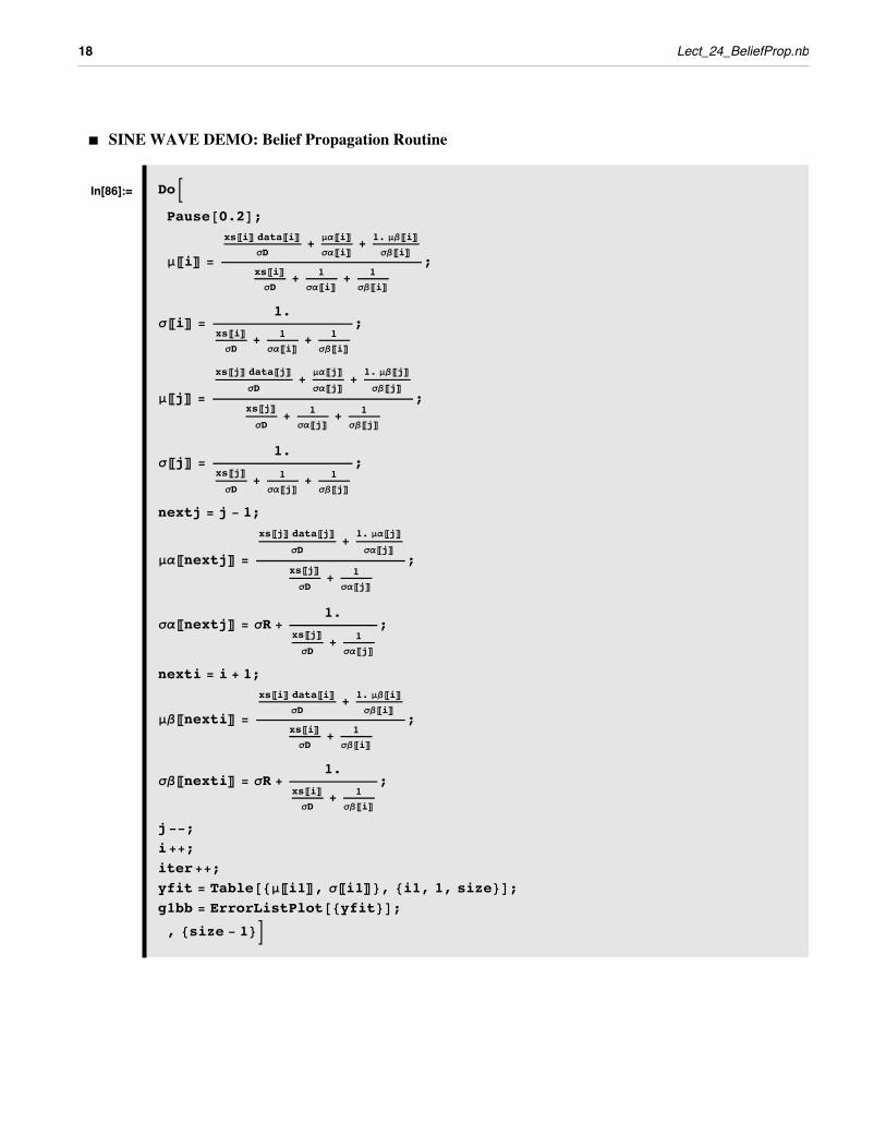
‡ SINE WAVE DEMO: Belief Propagation Routine

In[86]:= [email protected];

–PiT =

xsPiT dataPiTsD

+ –aPiTsaPiT + 1. –bPiT

sbPiTxsPiTsD

+ 1saPiT + 1

sbPiT

;

sPiT =1.

xsPiTsD

+ 1saPiT + 1

sbPiT

;

–PjT =

xsPjT dataPjTsD

+–aPjTsaPjT +

1. –bPjTsbPjT

xsPjTsD

+ 1saPjT + 1

sbPjT

;

sPjT =1.

xsPjTsD

+ 1saPjT + 1

sbPjT

;

nextj = j - 1;

–aPnextjT =

xsPjT dataPjTsD

+1. –aPjTsaPjT

xsPjTsD

+ 1saPjT

;

saPnextjT = sR +1.

xsPjTsD

+ 1saPjT

;

nexti = i + 1;

–bPnextiT =

xsPiT dataPiTsD

+ 1. –bPiTsbPiT

xsPiTsD

+ 1sbPiT

;

sbPnextiT = sR +1.

xsPiTsD

+ 1sbPiT

;

j--;i++;iter++;yfit = Table@8–Pi1T, sPi1T<, 8i1, 1, size<D;g1bb = ErrorListPlot@8yfit<D;, 8size - 1<F

References


ReferencesApplebaum, D. (1996). Probability and Information . Cambridge, UK: Cambridge University Press.

Frey, B. J. (1998). Graphical Models for Machine Learning and Digital Communication. Cambridge, Massachusetts: MIT Press.

Jepson, A., & Black, M. J. (1993). Mixture models for optical flow computation. Paper presented at the Proc. IEEE Conf. Comput. Vsion Pattern Recog., New York.

Kersten, D. and P.W. Schrater (2000), Pattern Inference Theory: A Probabilistic Approach to Vision, in Perception and the Physical World, R. Mausfeld and D. Heyer, Editors. , John Wiley & Sons, Ltd.: Chichester. (pdf)

Kersten, D., & Madarasmi, S. (1995). The Visual Perception of Surfaces, their Properties, and Relationships. DIMACS Series in Discrete Mathematics and Theoretical Computer Science, 19, 373-389.

Madarasmi, S., Kersten, D., & Pong, T.-C. (1993). The computation of stereo disparity for transparent and for opaque surfaces. In C. L. Giles & S. J. Hanson & J. D. Cowan (Eds.), Advances in Neural Information Processing Systems 5. San Mateo, CA: Morgan Kaufmann Publishers.

Pearl, Judea. (1997) Probabilistic Reasoning in Intelligent Systems : Networks of Plausible Inference. (amazon.com link)

Ripley, B. D. (1996). Pattern Reco gnition and Neural Networks. Cambridge, UK: Cambridge University Press.

Weiss Y. (1999) Bayesian Belief Propagation for Image Understanding submitted to SCTV 1999. (gzipped postscript 297K)

Weiss, Y. (1997). Smoothness in Layers: Motion segmentation using nonparametric mixture estimation. Paper presented at the Proceedings of IEEE conference on Computer Vision and Pattern Recognition.

Yuille, A., Coughlan J., Kersten D.(1998) (pdf)

For notes on Graphical Models, see:http://www.cs.berkeley.edu/~murphyk/Bayes/bayes.html

© 2000, 2001, 2003, 2005, 2007 Daniel Kersten, Computational Vision Lab, Department of Psychology, University of Minnesota. (http://vision.psych.umn.edu/www/kersten-lab/kersten-lab.html)


Documents

Introduction to Neural Networks U. Minn. Psy 5038 Daniel ...vision.psych.umn.edu/users/kersten/kersten-lab/courses/Psy5038WF… · Introduction to Neural Networks U. Minn. Psy 5038