Embed Size (px)
Citation preview
Algorithmic Intelligence Laboratory
Algorithmic Intelligence Laboratory
AI602: Recent Advances in Deep LearningLecture 1
Slide made by
Hyungwon Choi and Yunhun JangKAIST EE
Introduction to Neural Networks: DNN / CNN / RNN
Algorithmic Intelligence Laboratory
What is Machine/Deep Learning?
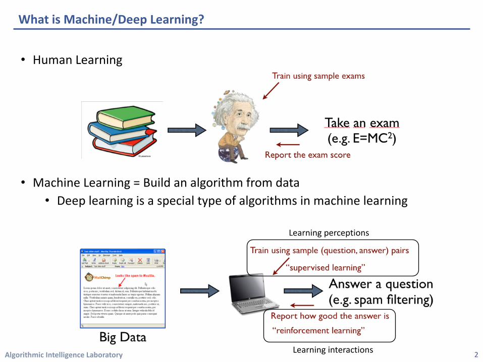
• Human Learning
• Machine Learning = Build an algorithm from data• Deep learning is a special type of algorithms in machine learning
2
Learning perceptions
Learning interactions
Algorithmic Intelligence Laboratory
Definition of Deep Learning
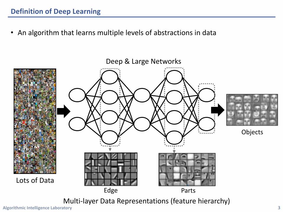
• An algorithm that learns multiple levels of abstractions in data
3
Lots of Data
Objects
Edge Parts
Deep & Large Networks
Multi-layer Data Representations (feature hierarchy)
Algorithmic Intelligence Laboratory
Deep Learning = Feature Learning
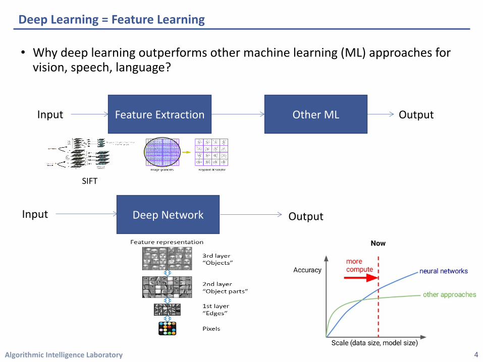
• Why deep learning outperforms other machine learning (ML) approaches for vision, speech, language?
Feature Extraction Other MLInput Output
Deep NetworkInput Output
SIFT
4
Algorithmic Intelligence Laboratory
1. Deep Neural Networks (DNN)• Basics • Training : Back propagation
2. Convolutional Neural Networks (CNN)• Basics• Convolution and pooling• Some applications
3. Recurrent Neural Networks (RNN)• Basics• Character-level language model (example)
4. Question• Why is it difficult to train a deep neural network?
Table of Contents
5
Algorithmic Intelligence Laboratory
1. Deep Neural Networks (DNN)• Basics• Training : Back propagation
2. Convolutional Neural Networks (CNN)• Basics• Convolution and pooling• Some applications
3. Recurrent Neural Networks (RNN)• Basics• Character-level language model (example)
4. Question• Why is it difficult to train a deep neural network?
Table of Contents
6
Algorithmic Intelligence Laboratory
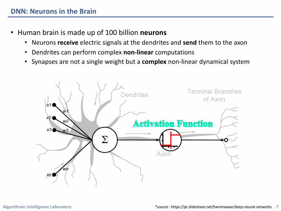
• Human brain is made up of 100 billion neurons• Neurons receive electric signals at the dendrites and send them to the axon• Dendrites can perform complex non-linear computations • Synapses are not a single weight but a complex non-linear dynamical system
DNN: Neurons in the Brain
7*source : https://pt.slideshare.net/hammawan/deep-neural-networks
Algorithmic Intelligence Laboratory
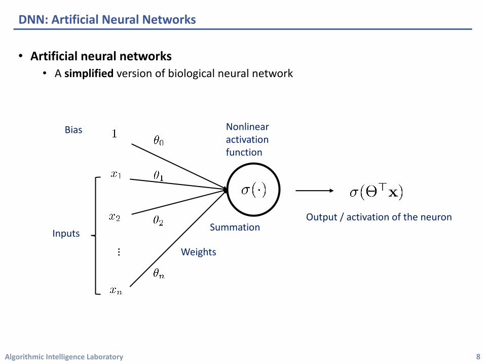
• Artificial neural networks• A simplified version of biological neural network
DNN: Artificial Neural Networks
8
Output / activation of the neuron
…
Bias
Inputs
Weights
Summation
Nonlinear activation function
Algorithmic Intelligence Laboratory
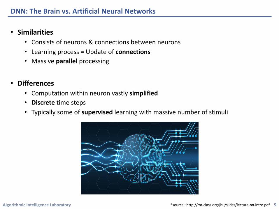
• Similarities• Consists of neurons & connections between neurons • Learning process = Update of connections• Massive parallel processing
• Differences• Computation within neuron vastly simplified• Discrete time steps • Typically some of supervised learning with massive number of stimuli
DNN: The Brain vs. Artificial Neural Networks
9*source : http://mt-class.org/jhu/slides/lecture-nn-intro.pdf
Algorithmic Intelligence Laboratory
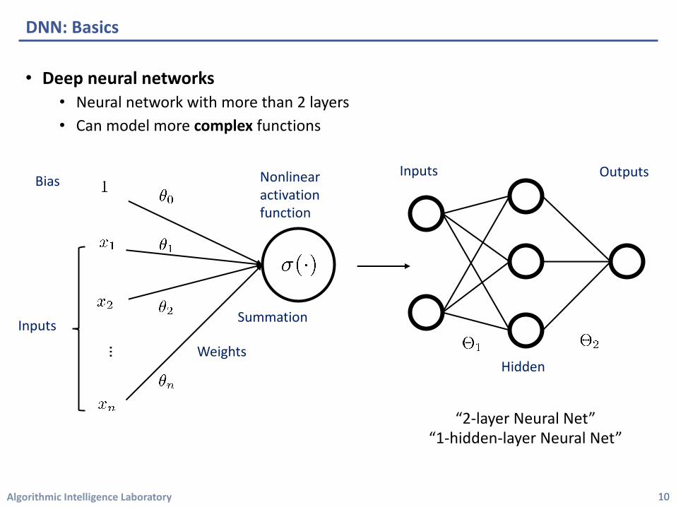
• Deep neural networks • Neural network with more than 2 layers• Can model more complex functions
DNN: Basics
10
Hidden
Inputs Outputs
“2-layer Neural Net” “1-hidden-layer Neural Net”
…
Bias
Inputs
Weights
Summation
Nonlinear activation function
Algorithmic Intelligence Laboratory
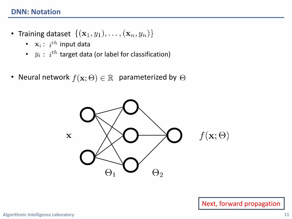
• Training dataset • : input data • : target data (or label for classification)
• Neural network parameterized by
DNN: Notation
11
Next, forward propagation
Algorithmic Intelligence Laboratory
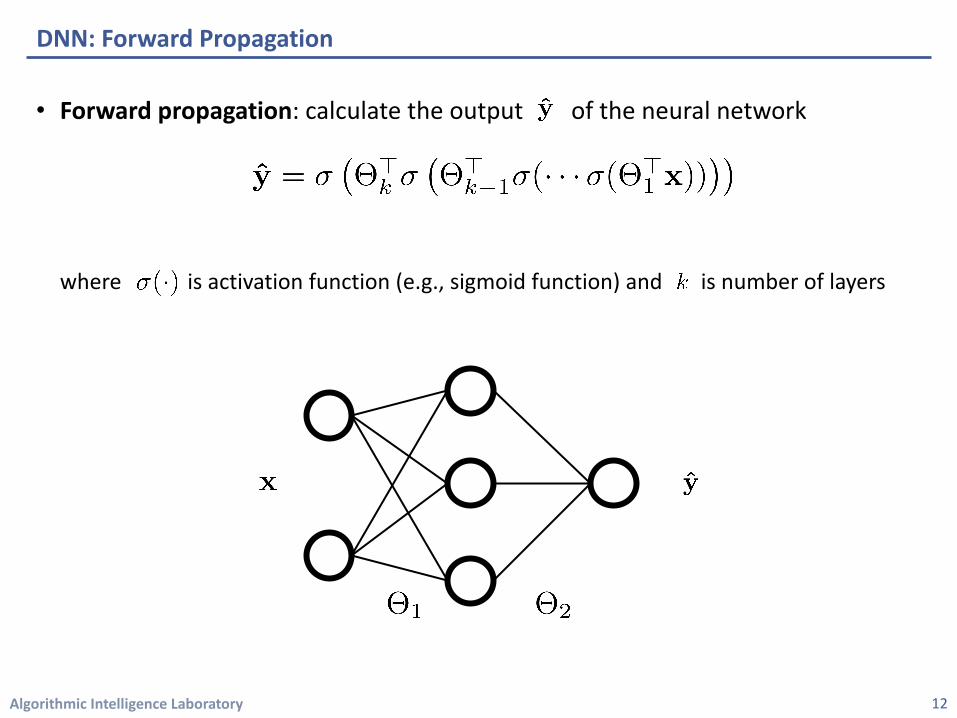
• Forward propagation: calculate the output of the neural network
where is activation function (e.g., sigmoid function) and is number of layers
DNN: Forward Propagation
12
Algorithmic Intelligence Laboratory
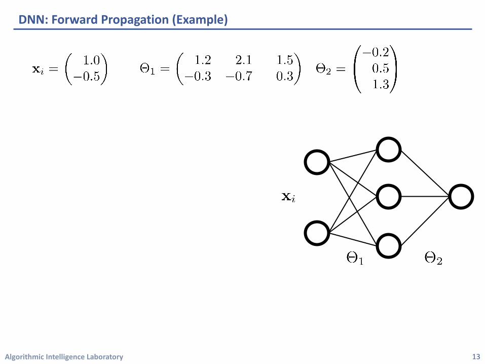
DNN: Forward Propagation (Example)
13
Algorithmic Intelligence Laboratory
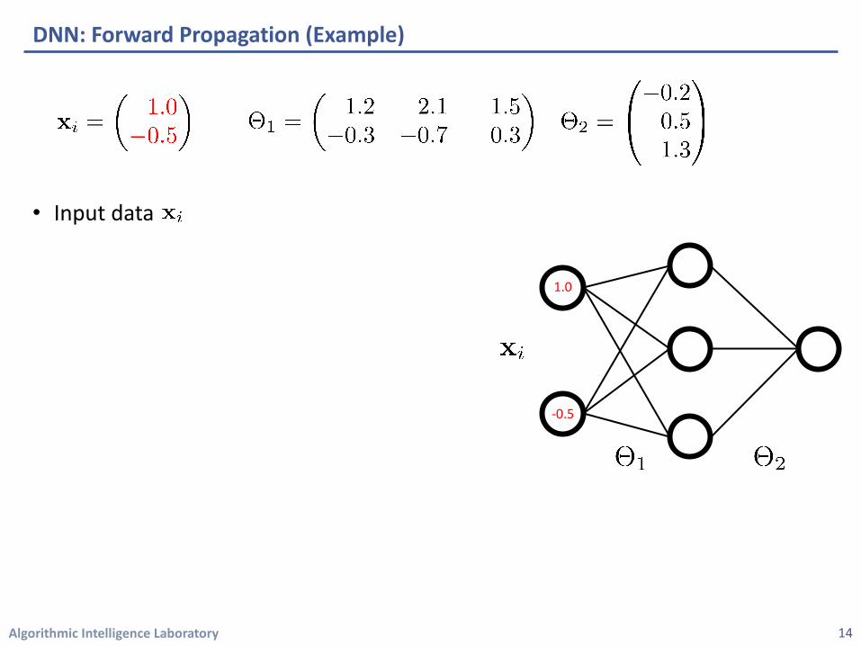
• Input data
DNN: Forward Propagation (Example)
14
1.0
-0.5
Algorithmic Intelligence Laboratory
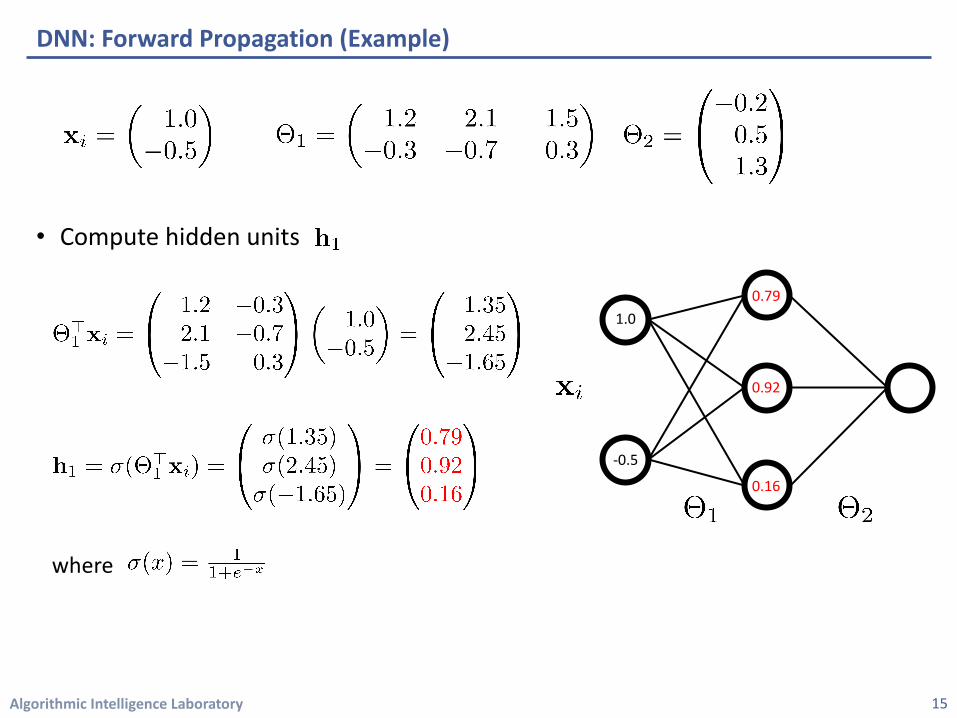
• Compute hidden units
DNN: Forward Propagation (Example)
15
0.79
0.92
0.16
1.0
-0.5
where
Algorithmic Intelligence Laboratory
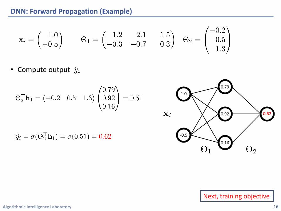
• Compute output
DNN: Forward Propagation (Example)
16
Next, training objective
0.79
0.92
0.16
1.0
-0.5
0.62
Algorithmic Intelligence Laboratory
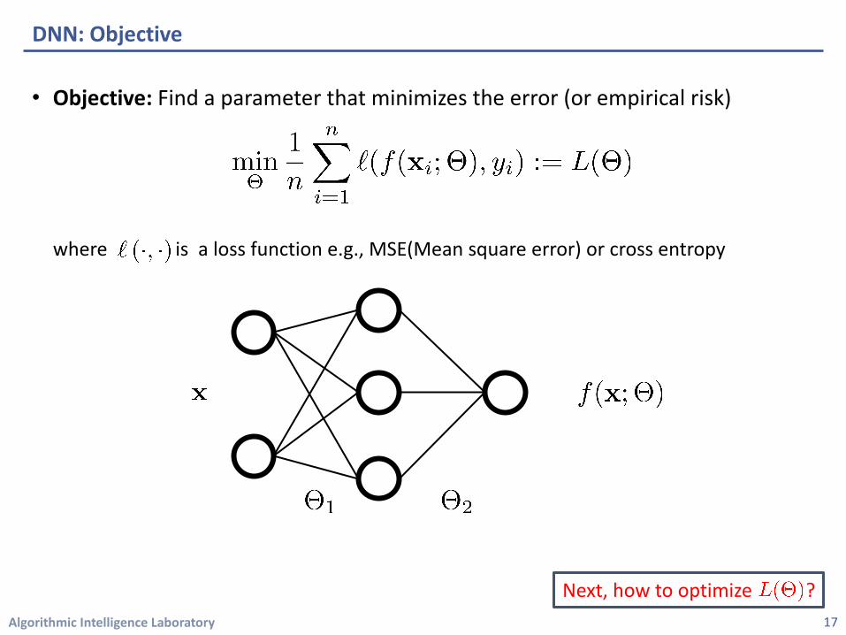
• Objective: Find a parameter that minimizes the error (or empirical risk)
where is a loss function e.g., MSE(Mean square error) or cross entropy
DNN: Objective
17
Next, how to optimize ?
Algorithmic Intelligence Laboratory
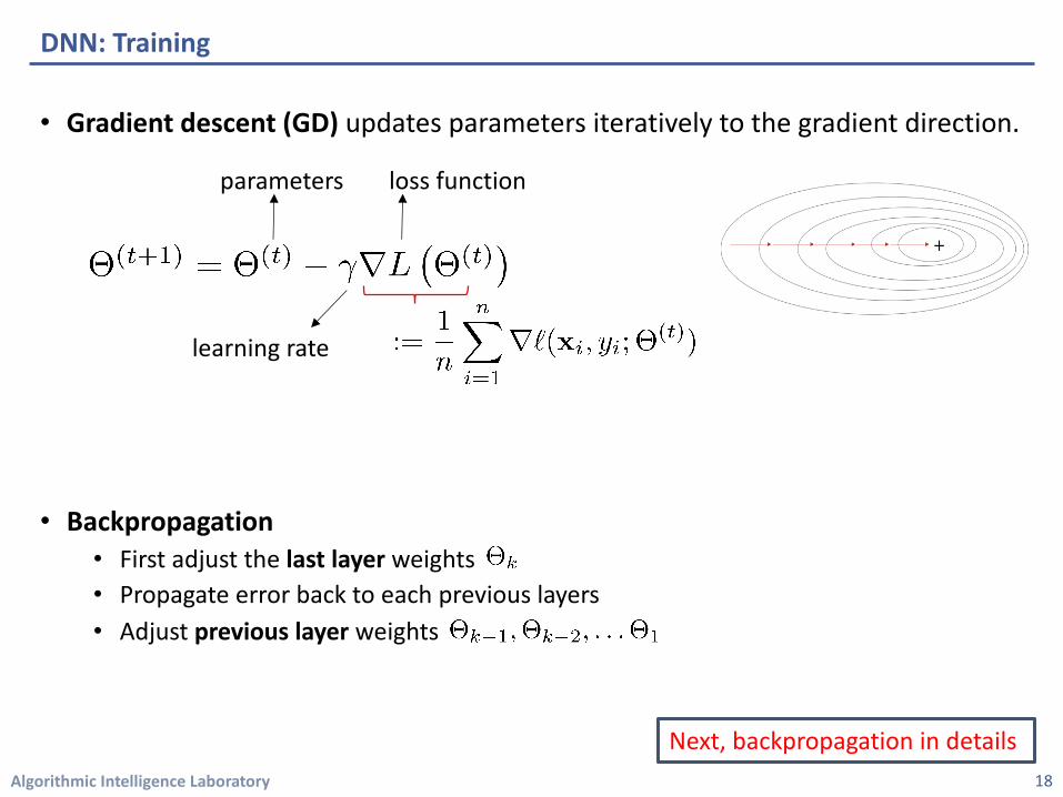
• Gradient descent (GD) updates parameters iteratively to the gradient direction.
• Backpropagation • First adjust the last layer weights• Propagate error back to each previous layers• Adjust previous layer weights
DNN: Training
18
parameters
learning rate
loss function
Next, backpropagation in details
Algorithmic Intelligence Laboratory
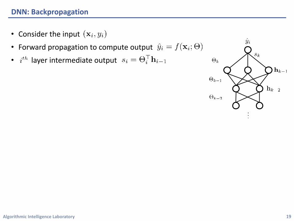
DNN: Backpropagation
19
• Consider the input
• Forward propagation to compute output
• layer intermediate output
Algorithmic Intelligence Laboratory
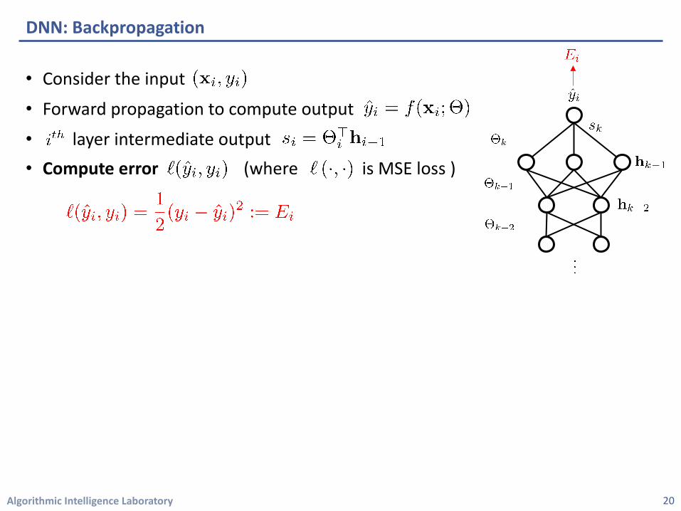
DNN: Backpropagation
20
• Consider the input
• Forward propagation to compute output
• layer intermediate output • Compute error (where is MSE loss )
Algorithmic Intelligence Laboratory
DNN: Backpropagation
21
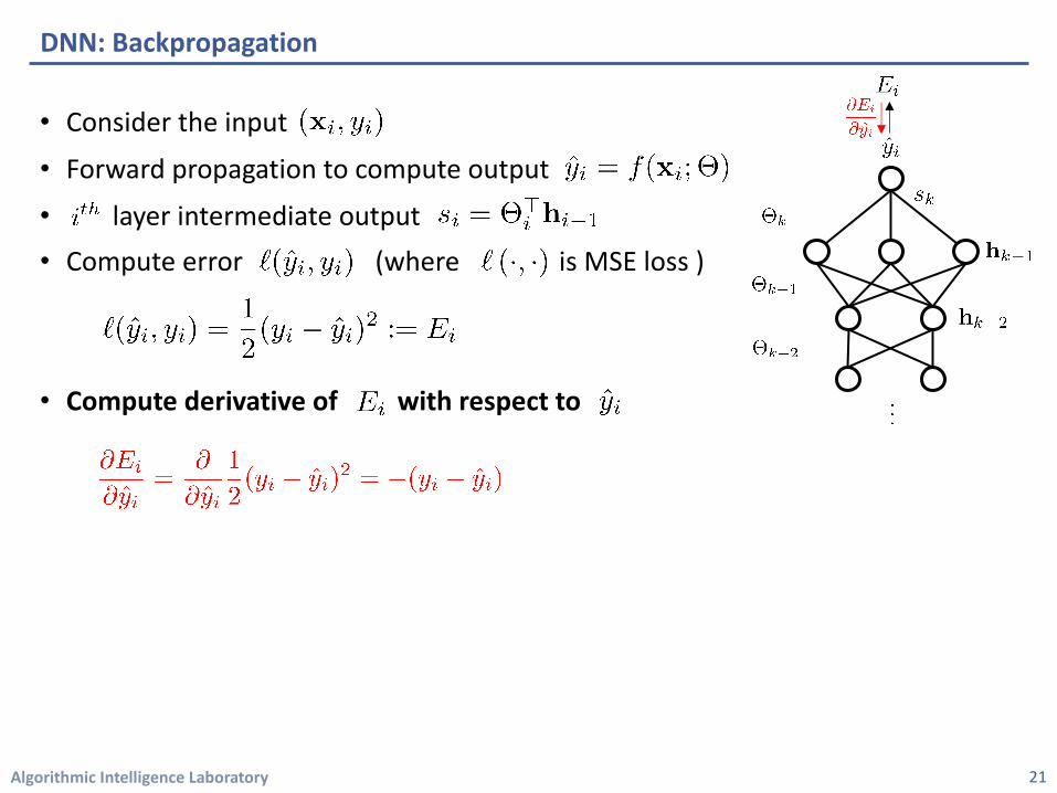
• Consider the input
• Forward propagation to compute output
• layer intermediate output • Compute error (where is MSE loss )
• Compute derivative of with respect to
Algorithmic Intelligence Laboratory
DNN: Backpropagation
22
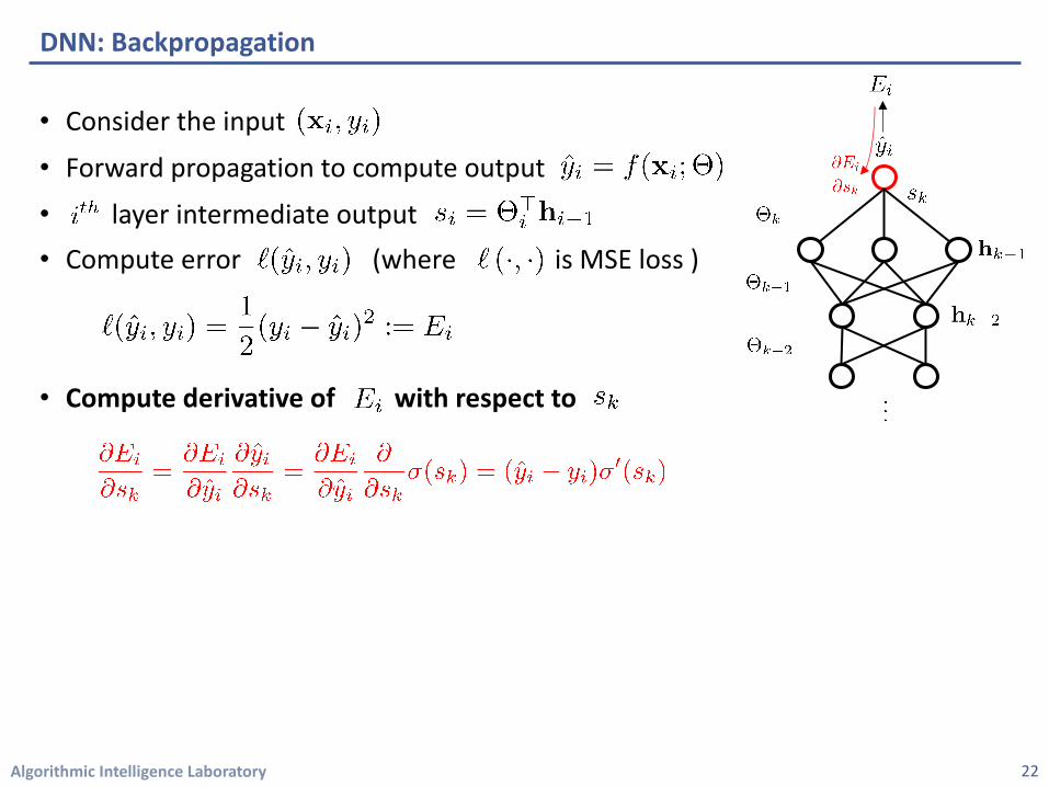
• Consider the input
• Forward propagation to compute output
• layer intermediate output • Compute error (where is MSE loss )
• Compute derivative of with respect to
Algorithmic Intelligence Laboratory
DNN: Backpropagation
23
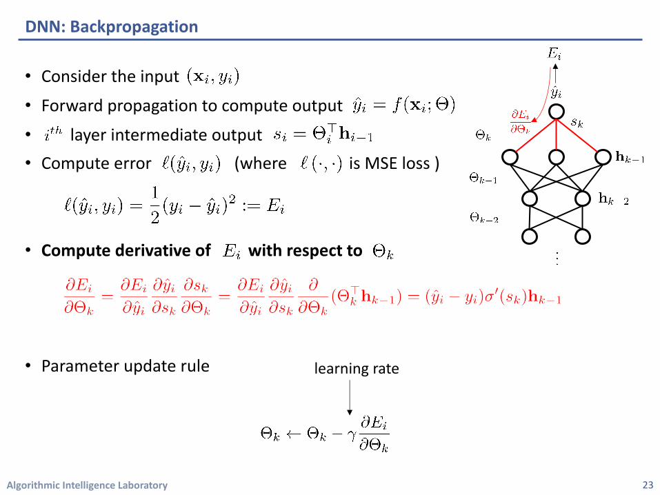
• Consider the input
• Forward propagation to compute output
• layer intermediate output • Compute error (where is MSE loss )
• Compute derivative of with respect to
• Parameter update rule learning rate
Algorithmic Intelligence Laboratory
DNN: Backpropagation
24
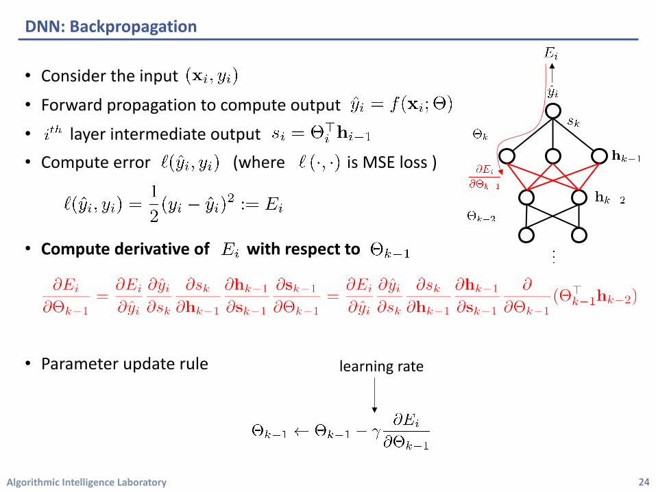
• Consider the input
• Forward propagation to compute output
• layer intermediate output • Compute error (where is MSE loss )
• Compute derivative of with respect to
• Parameter update rule learning rate
Algorithmic Intelligence Laboratory
DNN: Backpropagation
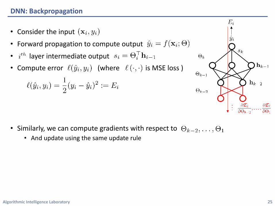
25
• Consider the input
• Forward propagation to compute output
• layer intermediate output • Compute error (where is MSE loss )
• Similarly, we can compute gradients with respect to • And update using the same update rule
Algorithmic Intelligence Laboratory
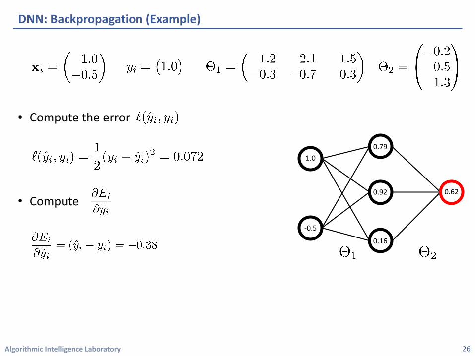
• Compute the error
• Compute
DNN: Backpropagation (Example)
26
0.79
0.92
0.16
1.0
-0.5
0.62
Algorithmic Intelligence Laboratory
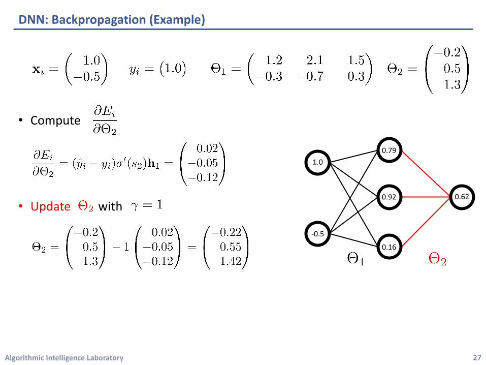
• Compute
• Update with
DNN: Backpropagation (Example)
27
0.79
0.92
0.16
1.0
-0.5
0.62
Algorithmic Intelligence Laboratory
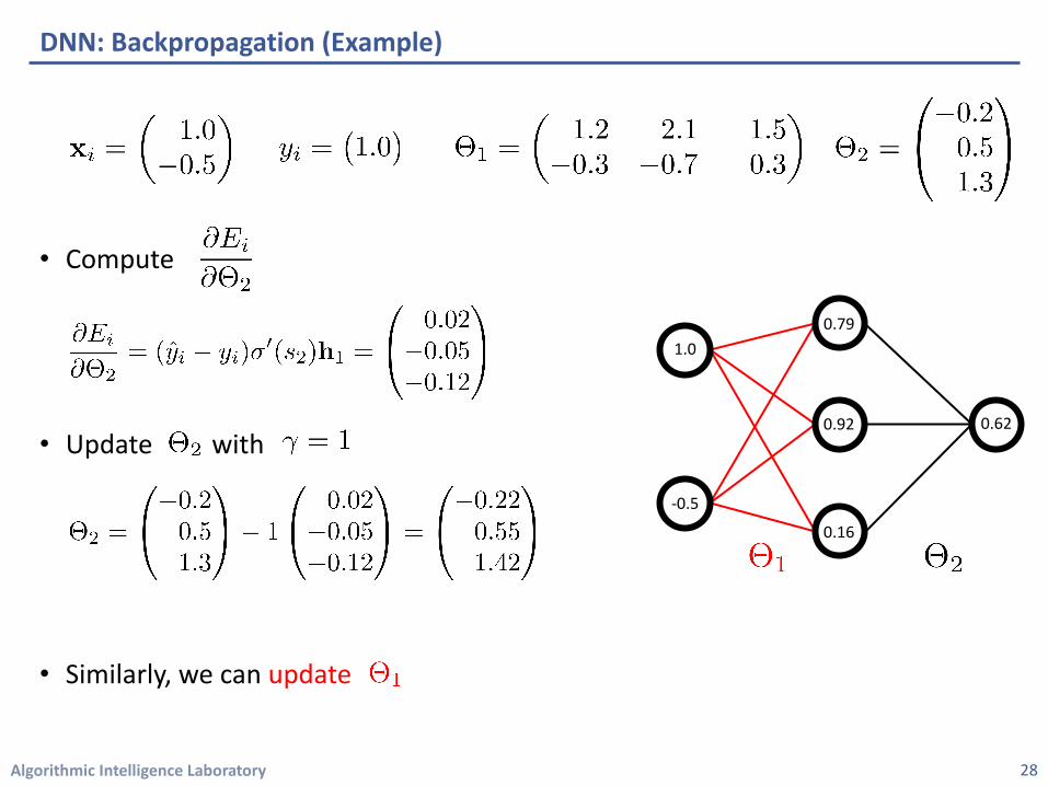
• Compute
• Update with
• Similarly, we can update
DNN: Backpropagation (Example)
28
0.79
0.16
1.0
-0.5
0.620.92
Algorithmic Intelligence Laboratory
1. Deep Neural Networks (DNN)• Basics • Training : Back propagation
2. Convolutional Neural Networks (CNN)• Basics• Convolution and Pooling• Some applications
3. Recurrent Neural Networks (RNN)• Basics• Character-level language model (example)
4. Question• Why is it difficult to train a deep neural network?
Table of Contents
29
Algorithmic Intelligence Laboratory
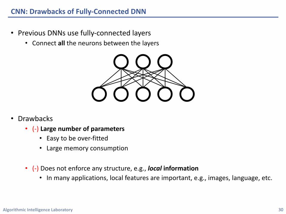
• Previous DNNs use fully-connected layers• Connect all the neurons between the layers
• Drawbacks• (-) Large number of parameters
• Easy to be over-fitted• Large memory consumption
• (-) Does not enforce any structure, e.g., local information• In many applications, local features are important, e.g., images, language, etc.
CNN: Drawbacks of Fully-Connected DNN
30
Algorithmic Intelligence Laboratory
CNN: Basics
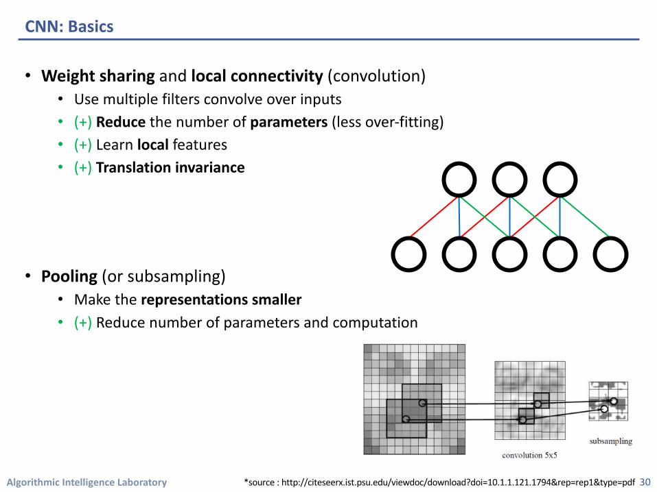
• Weight sharing and local connectivity (convolution)• Use multiple filters convolve over inputs • (+) Reduce the number of parameters (less over-fitting)• (+) Learn local features• (+) Translation invariance
• Pooling (or subsampling)• Make the representations smaller• (+) Reduce number of parameters and computation
30*source : http://citeseerx.ist.psu.edu/viewdoc/download?doi=10.1.1.121.1794&rep=rep1&type=pdf
Algorithmic Intelligence Laboratory
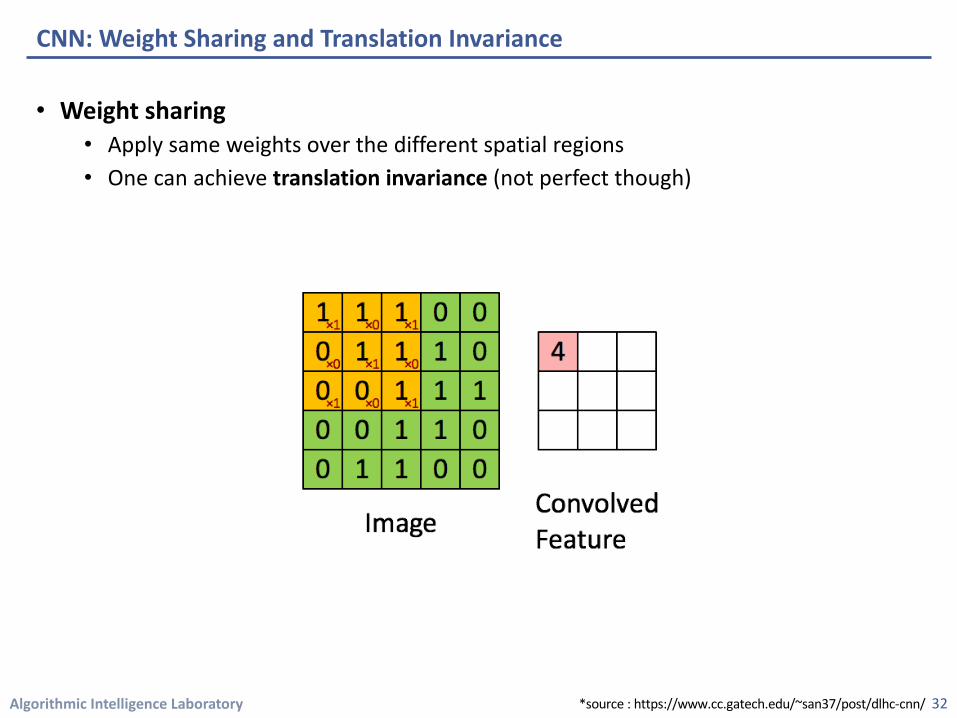
• Weight sharing• Apply same weights over the different spatial regions• One can achieve translation invariance (not perfect though)
CNN: Weight Sharing and Translation Invariance
32*source : https://www.cc.gatech.edu/~san37/post/dlhc-cnn/
Algorithmic Intelligence Laboratory
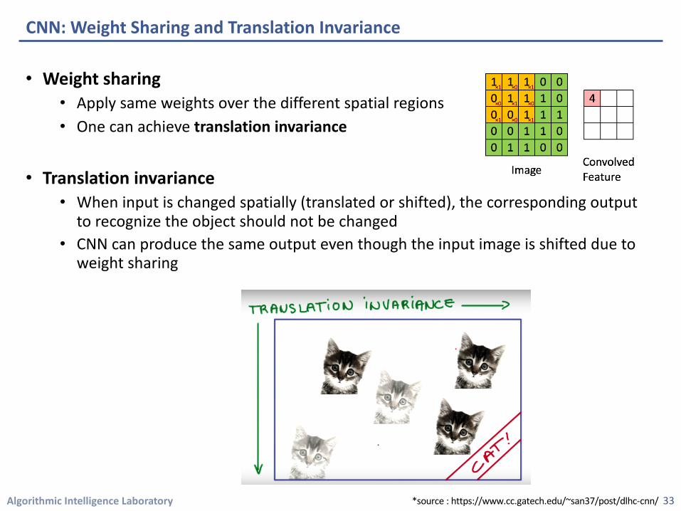
• Weight sharing• Apply same weights over the different spatial regions• One can achieve translation invariance
• Translation invariance • When input is changed spatially (translated or shifted), the corresponding output
to recognize the object should not be changed • CNN can produce the same output even though the input image is shifted due to
weight sharing
CNN: Weight Sharing and Translation Invariance
33*source : https://www.cc.gatech.edu/~san37/post/dlhc-cnn/
Algorithmic Intelligence Laboratory
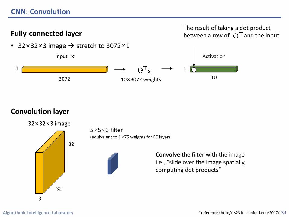
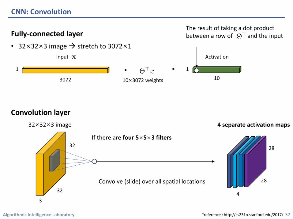
Fully-connected layer• 32×32×3 image à stretch to 3072×1
Convolution layer
CNN: Convolution
34
Input
1
3072 10×3072 weights
Activation
110
The result of taking a dot product between a row of and the input
3
32
32
32×32×3 image 5×5×3 filter(equivalent to 1×75 weights for FC layer)
Convolve the filter with the imagei.e., “slide over the image spatially, computing dot products”
*reference : http://cs231n.stanford.edu/2017/
Algorithmic Intelligence Laboratory
Fully-connected layer• 32×32×3 image à stretch to 3072×1
Convolution layer
CNN: Convolution
35
1
3072 10×3072 weights
Activation
110
3
32
32
32×32×3 image
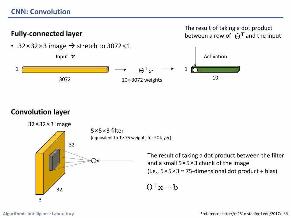
The result of taking a dot product between the filter and a small 5×5×3 chunk of the image(i.e., 5×5×3 = 75-dimensional dot product + bias)
5×5×3 filter(equivalent to 1×75 weights for FC layer)
Input
The result of taking a dot product between a row of and the input
*reference : http://cs231n.stanford.edu/2017/
Algorithmic Intelligence Laboratory
Fully-connected layer• 32×32×3 image à stretch to 3072×1
Convolution layer
CNN: Convolution
36
1
3072 10×3072 weights
Activation
110
3
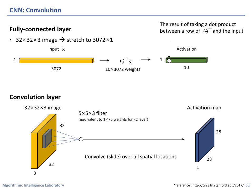
32Convolve (slide) over all spatial locations
32
32×32×3 image Activation map
1
28
28
5×5×3 filter(equivalent to 1×75 weights for FC layer)
Input
The result of taking a dot product between a row of and the input
*reference : http://cs231n.stanford.edu/2017/
Algorithmic Intelligence Laboratory
Fully-connected layer• 32×32×3 image à stretch to 3072×1
Convolution layer
CNN: Convolution
37
1
3072 10×3072 weights
Activation
110
3
32
If there are four 5×5×3 filters
Convolve (slide) over all spatial locations
32
32×32×3 image 4 separate activation maps
4
28
28
Input
The result of taking a dot product between a row of and the input
*reference : http://cs231n.stanford.edu/2017/

Algorithmic Intelligence Laboratory
• Closer look at spatial dimensions
CNN: An Example
38
7
7
7×7 input (spatially)Assume 3×3 filterApplied with stride 1
*reference : http://cs231n.stanford.edu/2017/
Algorithmic Intelligence Laboratory
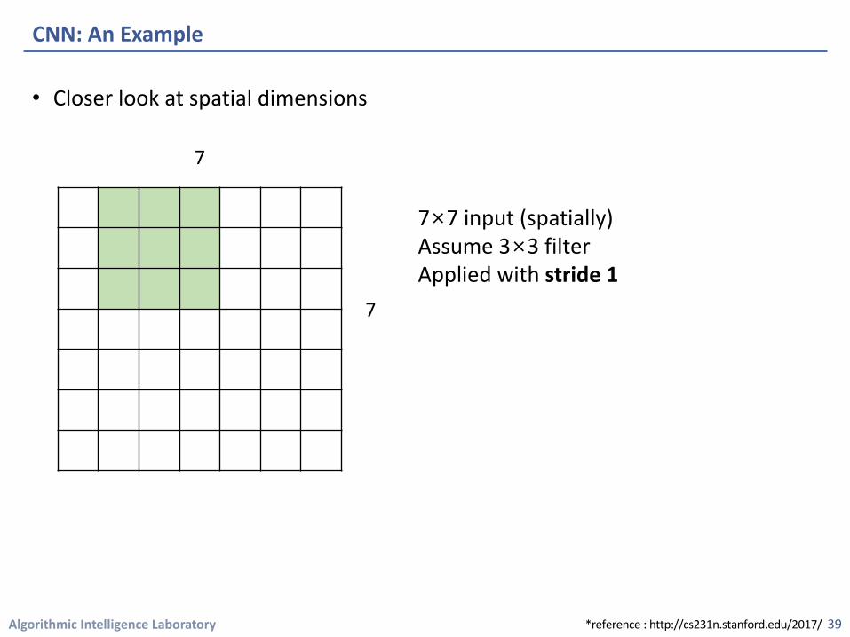
• Closer look at spatial dimensions
CNN: An Example
39
7
7
7×7 input (spatially)Assume 3×3 filterApplied with stride 1
*reference : http://cs231n.stanford.edu/2017/
Algorithmic Intelligence Laboratory
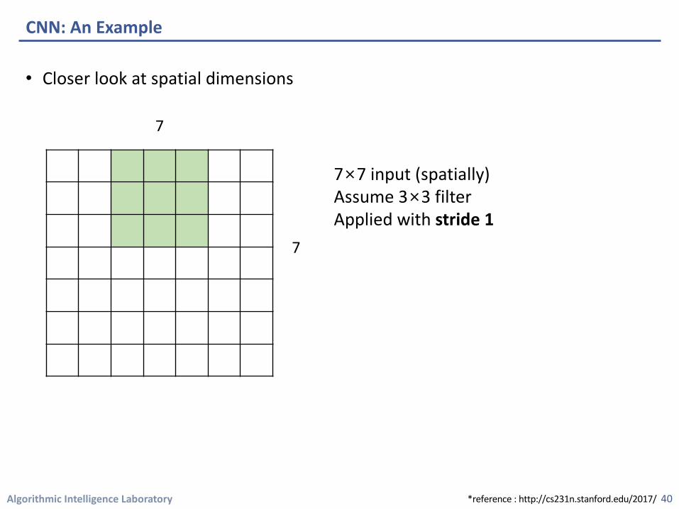
• Closer look at spatial dimensions
CNN: An Example
40
7
7
7×7 input (spatially)Assume 3×3 filterApplied with stride 1
*reference : http://cs231n.stanford.edu/2017/
Algorithmic Intelligence Laboratory
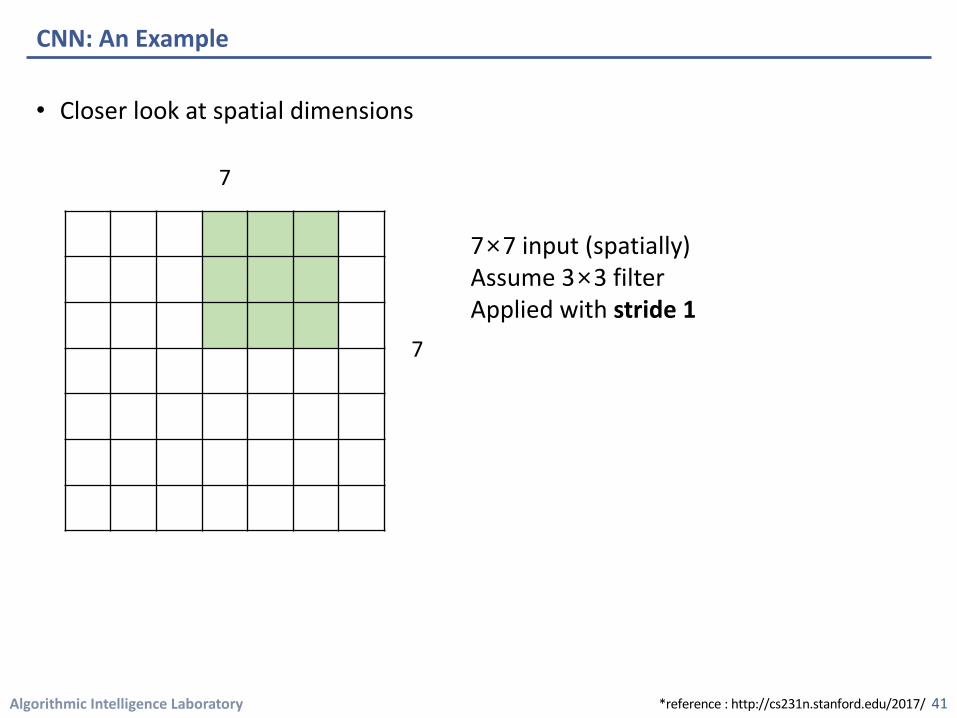
• Closer look at spatial dimensions
CNN: An Example
41
7
7
7×7 input (spatially)Assume 3×3 filterApplied with stride 1
*reference : http://cs231n.stanford.edu/2017/

Algorithmic Intelligence Laboratory
• Closer look at spatial dimensions
CNN: An Example
42
7
7
7×7 input (spatially)Assume 3×3 filterApplied with stride 1
à 5×5 output
*reference : http://cs231n.stanford.edu/2017/
Algorithmic Intelligence Laboratory
• Closer look at spatial dimensions
CNN: An Example
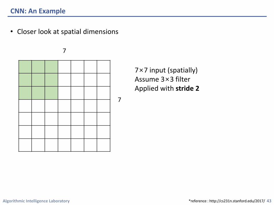
43
7
7
7×7 input (spatially)Assume 3×3 filter Applied with stride 2
*reference : http://cs231n.stanford.edu/2017/

Algorithmic Intelligence Laboratory
• Closer look at spatial dimensions
CNN: An Example
44
7
7
7×7 input (spatially)Assume 3×3 filter Applied with stride 2
*reference : http://cs231n.stanford.edu/2017/
Algorithmic Intelligence Laboratory
• Closer look at spatial dimensions
CNN: An Example
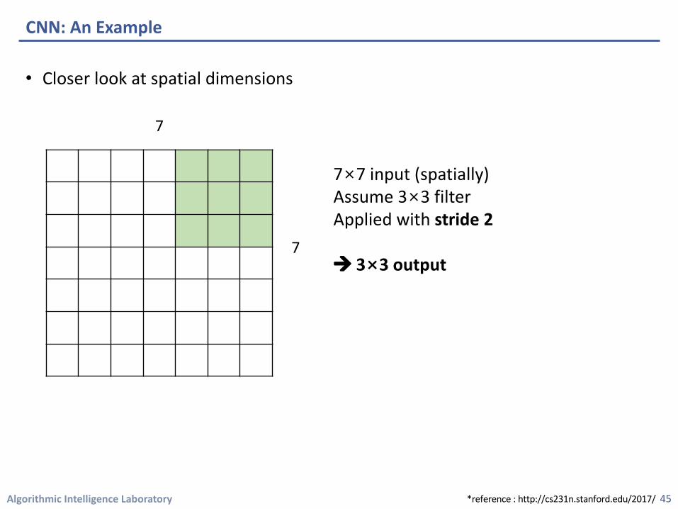
45
7
7
7×7 input (spatially)Assume 3×3 filter Applied with stride 2
à 3×3 output
*reference : http://cs231n.stanford.edu/2017/
Algorithmic Intelligence Laboratory
• Closer look at spatial dimensions
CNN: An Example
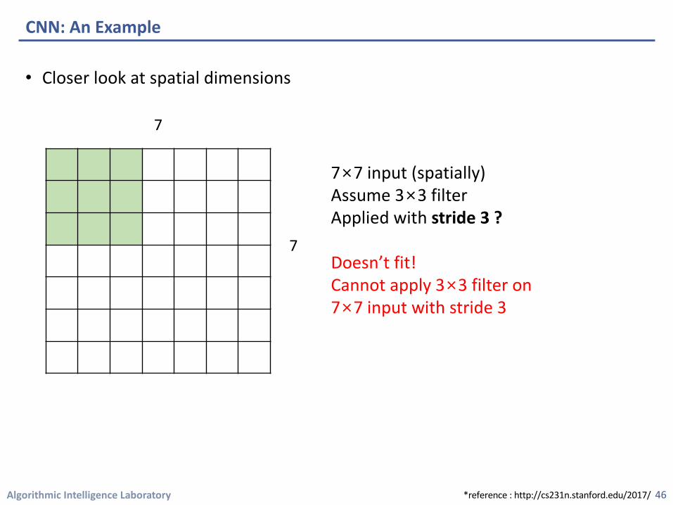
46
7
7
7×7 input (spatially)Assume 3×3 filter Applied with stride 3 ?
Doesn’t fit!Cannot apply 3×3 filter on 7×7 input with stride 3
*reference : http://cs231n.stanford.edu/2017/
Algorithmic Intelligence Laboratory
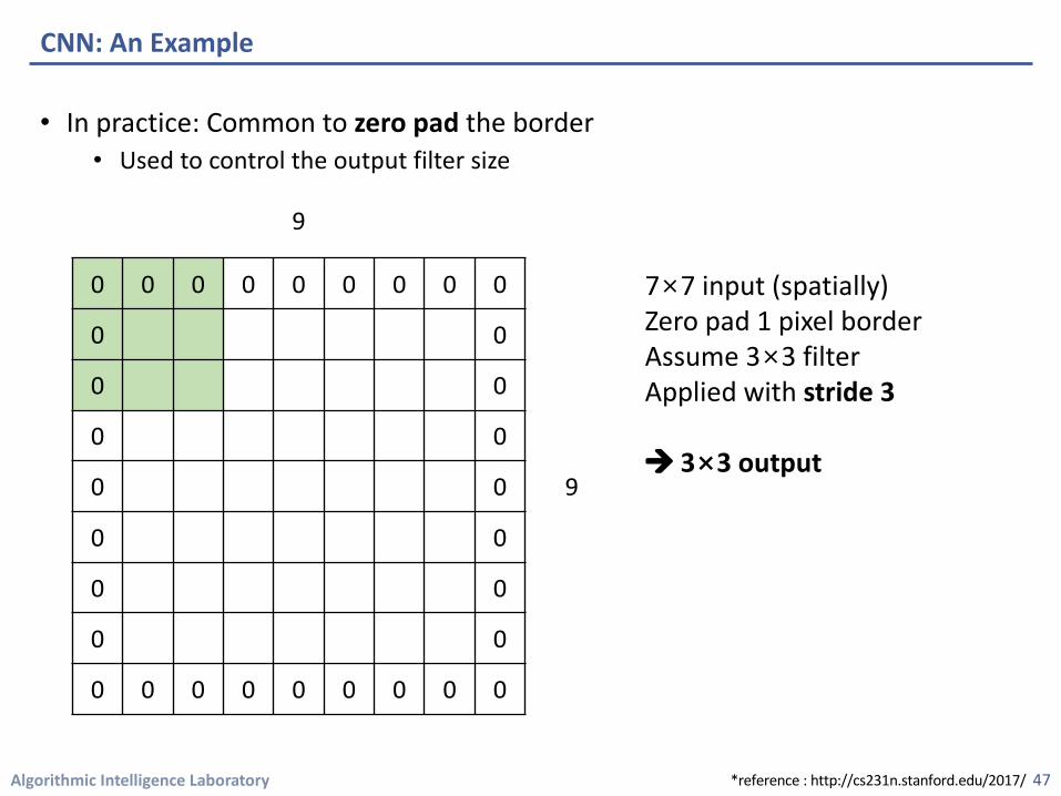
• In practice: Common to zero pad the border • Used to control the output filter size
CNN: An Example
47
9
7×7 input (spatially)Zero pad 1 pixel borderAssume 3×3 filter Applied with stride 3
à 3×3 output
0 0 0 0 0 0 0 0 0
0 0
0 0
0 0
0 0
0 0
0 0
0 0
0 0 0 0 0 0 0 0 0
9
*reference : http://cs231n.stanford.edu/2017/
Algorithmic Intelligence Laboratory
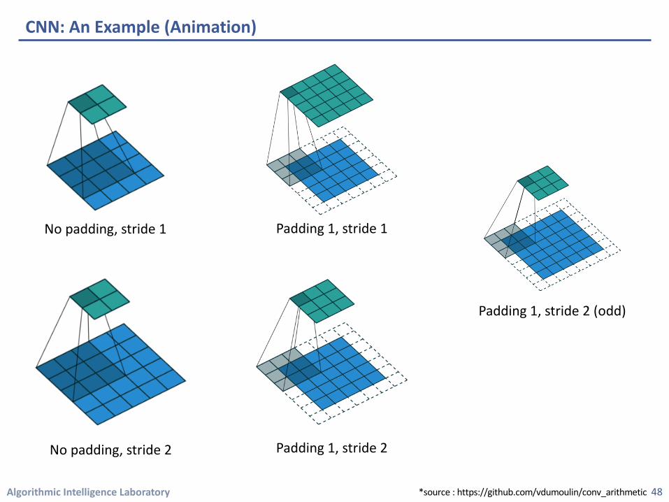
CNN: An Example (Animation)
48*source : https://github.com/vdumoulin/conv_arithmetic
No padding, stride 1
No padding, stride 2
Padding 1, stride 1
Padding 1, stride 2
Padding 1, stride 2 (odd)
Algorithmic Intelligence Laboratory
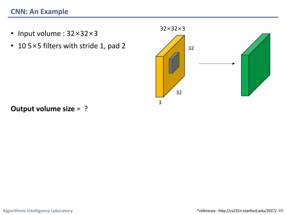
• Input volume : 32×32×3• 10 5×5 filters with stride 1, pad 2
Output volume size = ?
CNN: An Example
49
3
32
32
32×32×3
*reference : http://cs231n.stanford.edu/2017/
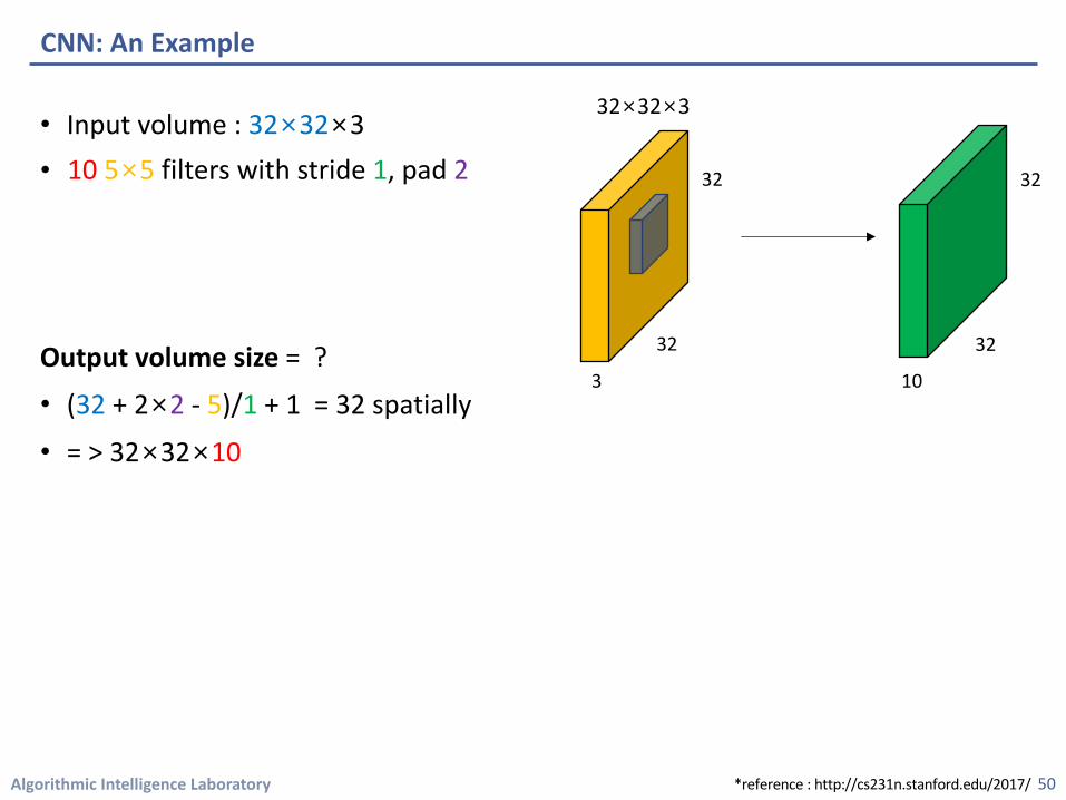
Algorithmic Intelligence Laboratory
• Input volume : 32×32×3•
Output volume size = ?
• (32 + 2×2 - 5)/1 + 1 = 32 spatially
• = > 32×32×10
CNN: An Example
50
3
32
32
32×32×3
10
32
32
*reference : http://cs231n.stanford.edu/2017/
10 5×5 filters with stride 1, pad 2
Algorithmic Intelligence Laboratory
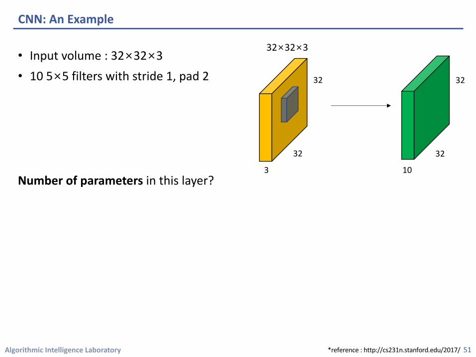
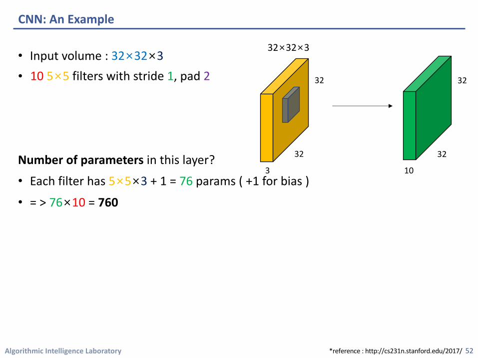
• Input volume : 32×32×3• 10 5×5 filters with stride 1, pad 2
Number of parameters in this layer?
CNN: An Example
51
3
32
32
32×32×3
10
32
32
*reference : http://cs231n.stanford.edu/2017/
Algorithmic Intelligence Laboratory
• Input volume : 32×32×3•
Number of parameters in this layer?
• Each filter has 5×5×3 + 1 = 76 params ( +1 for bias )
• = > 76×10 = 760
CNN: An Example
52
3
32
32
32×32×3
10
32
32
*reference : http://cs231n.stanford.edu/2017/
10 5×5 filters with stride 1, pad 2
Algorithmic Intelligence Laboratory
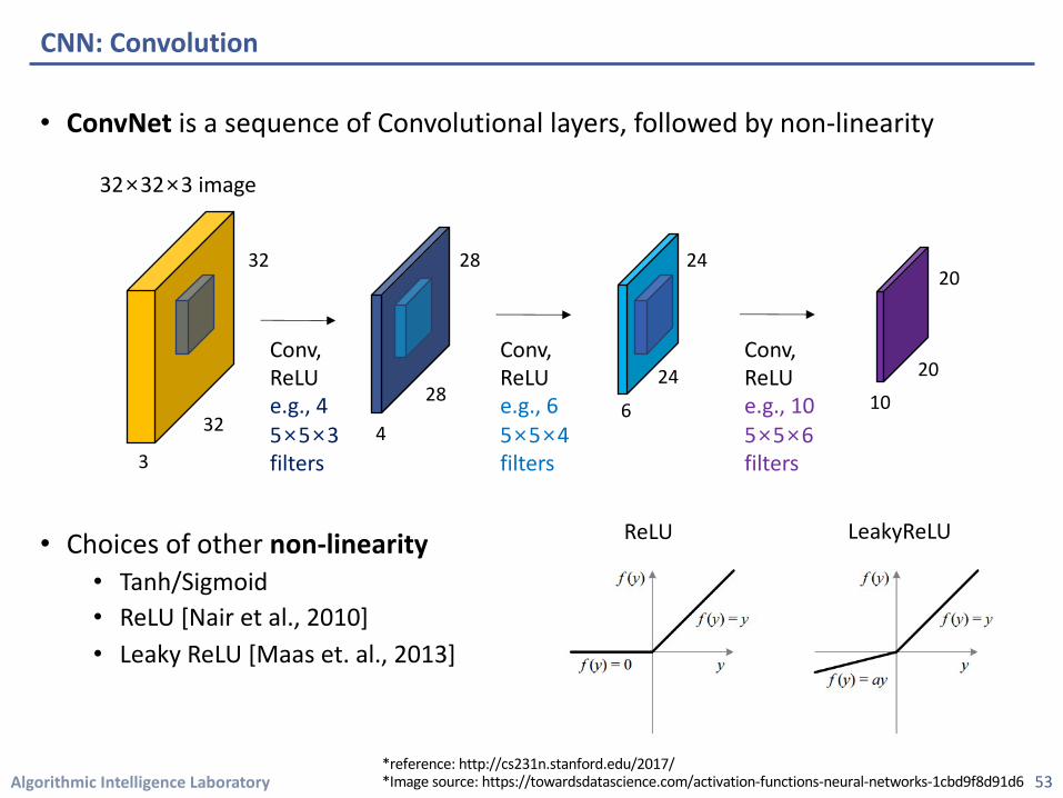
• ConvNet is a sequence of Convolutional layers, followed by non-linearity
• Choices of other non-linearity • Tanh/Sigmoid• ReLU [Nair et al., 2010]• Leaky ReLU [Maas et. al., 2013]
CNN: Convolution
53
3
32
32
32×32×3 image
4
28
28
Conv,ReLUe.g., 45×5×3filters
Conv,ReLUe.g., 65×5×4filters
6
24
24
Conv,ReLUe.g., 105×5×6filters
10
20
20
*reference: http://cs231n.stanford.edu/2017/*Image source: https://towardsdatascience.com/activation-functions-neural-networks-1cbd9f8d91d6
ReLU LeakyReLU
Algorithmic Intelligence Laboratory
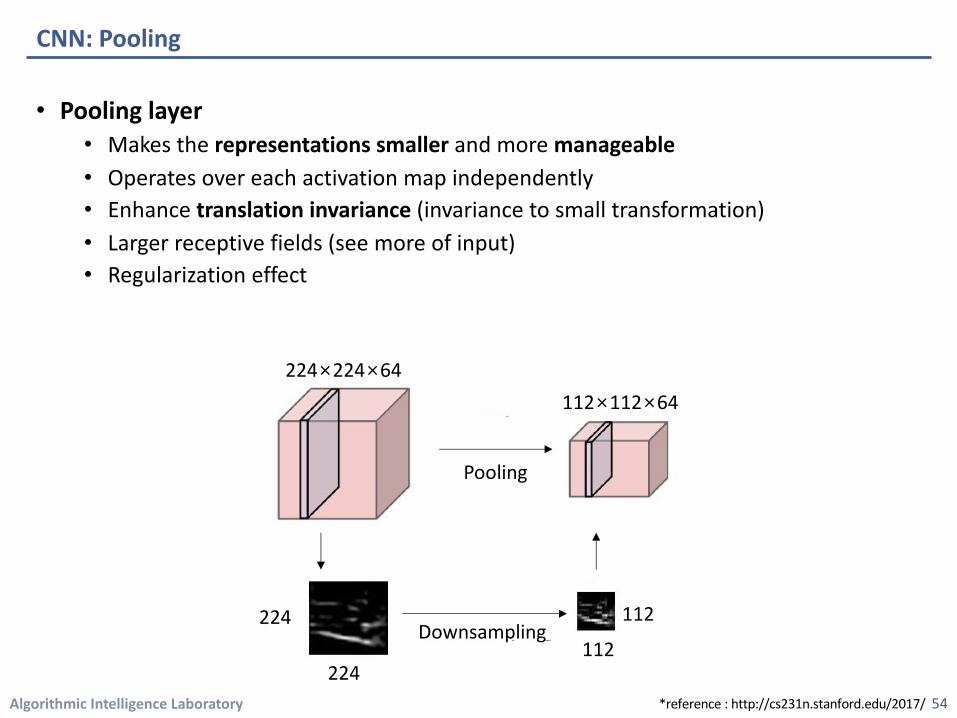
• Pooling layer• Makes the representations smaller and more manageable• Operates over each activation map independently • Enhance translation invariance (invariance to small transformation) • Larger receptive fields (see more of input)• Regularization effect
CNN: Pooling
54
224×224×64
224112
112Downsampling
Pooling
112×112×64
224*reference : http://cs231n.stanford.edu/2017/
Algorithmic Intelligence Laboratory
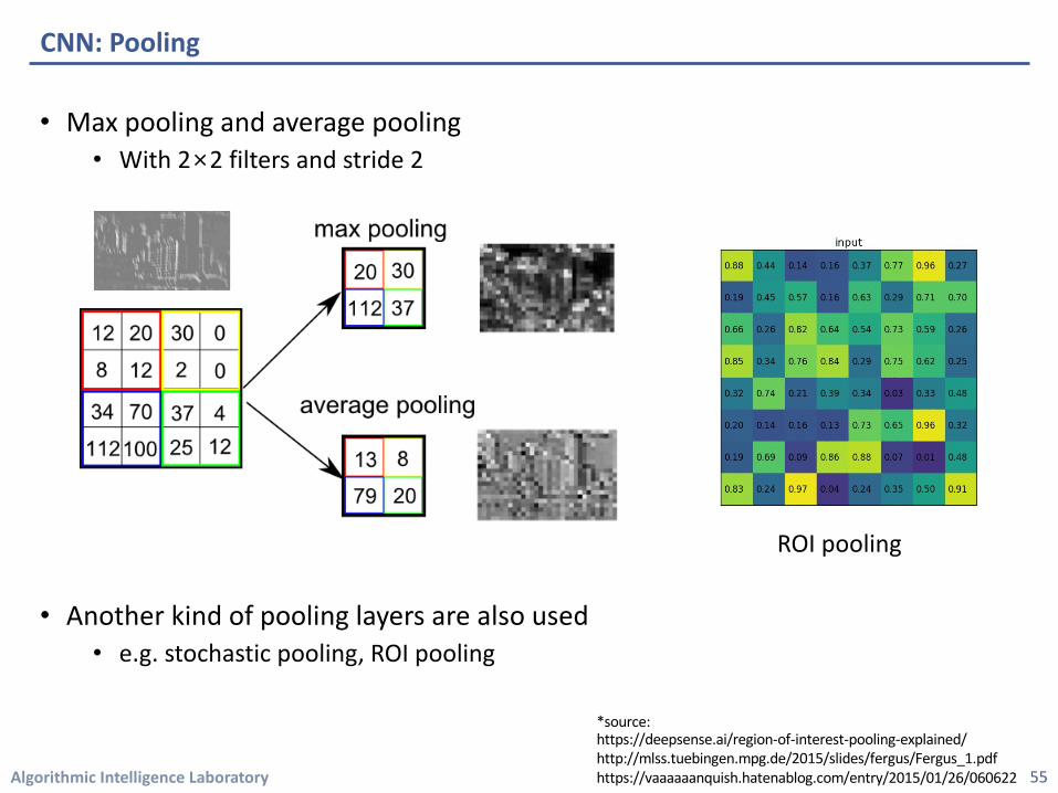
• Max pooling and average pooling • With 2×2 filters and stride 2
• Another kind of pooling layers are also used• e.g. stochastic pooling, ROI pooling
CNN: Pooling
55
ROI pooling
*source: https://deepsense.ai/region-of-interest-pooling-explained/http://mlss.tuebingen.mpg.de/2015/slides/fergus/Fergus_1.pdfhttps://vaaaaaanquish.hatenablog.com/entry/2015/01/26/060622
Algorithmic Intelligence Laboratory
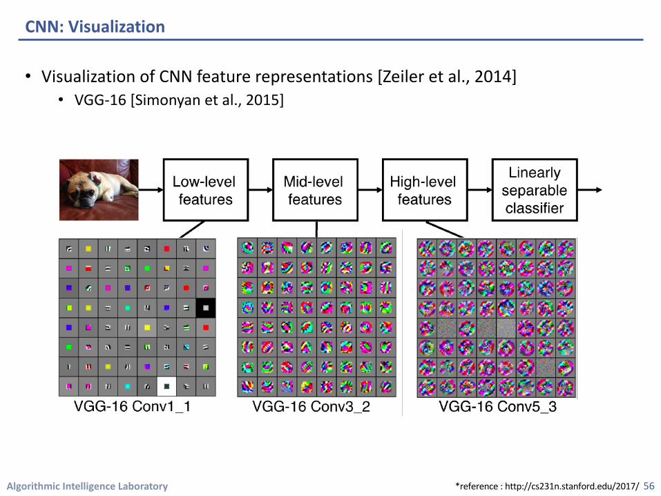
• Visualization of CNN feature representations [Zeiler et al., 2014]• VGG-16 [Simonyan et al., 2015]
CNN: Visualization
56*reference : http://cs231n.stanford.edu/2017/
Algorithmic Intelligence Laboratory
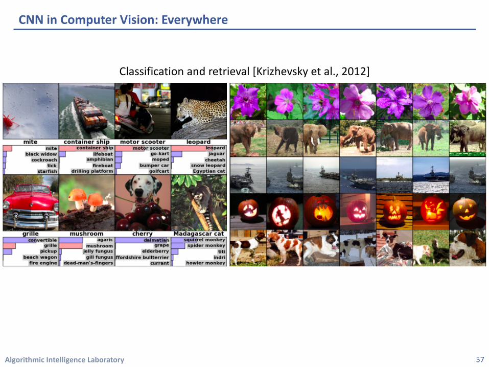
CNN in Computer Vision: Everywhere
57
Classification and retrieval [Krizhevsky et al., 2012]
Algorithmic Intelligence Laboratory
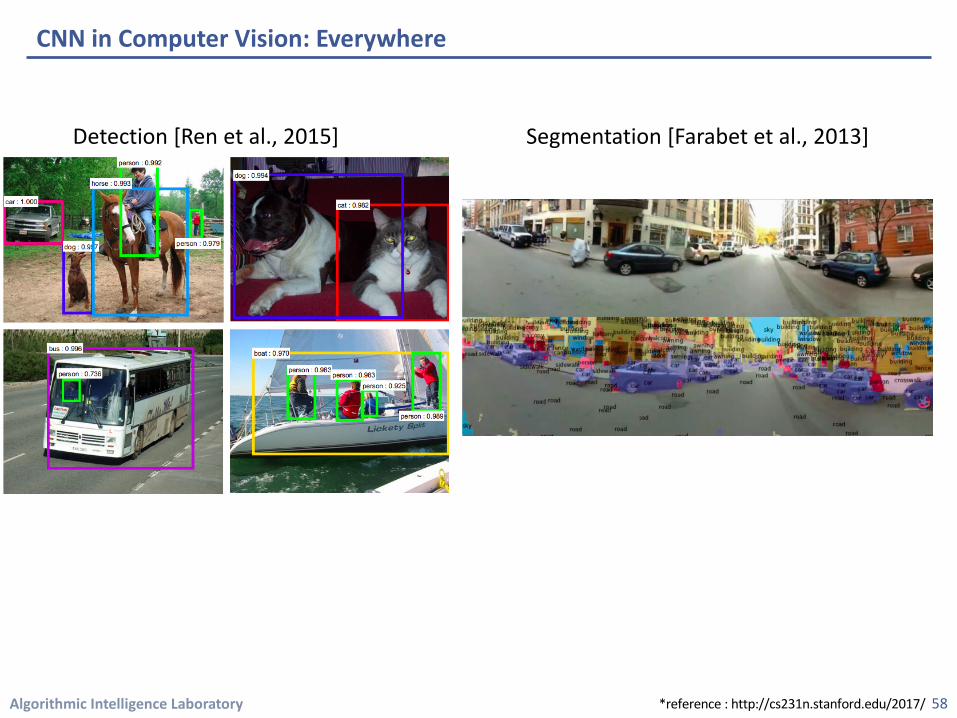
CNN in Computer Vision: Everywhere
58
Detection [Ren et al., 2015] Segmentation [Farabet et al., 2013]
*reference : http://cs231n.stanford.edu/2017/
Algorithmic Intelligence Laboratory
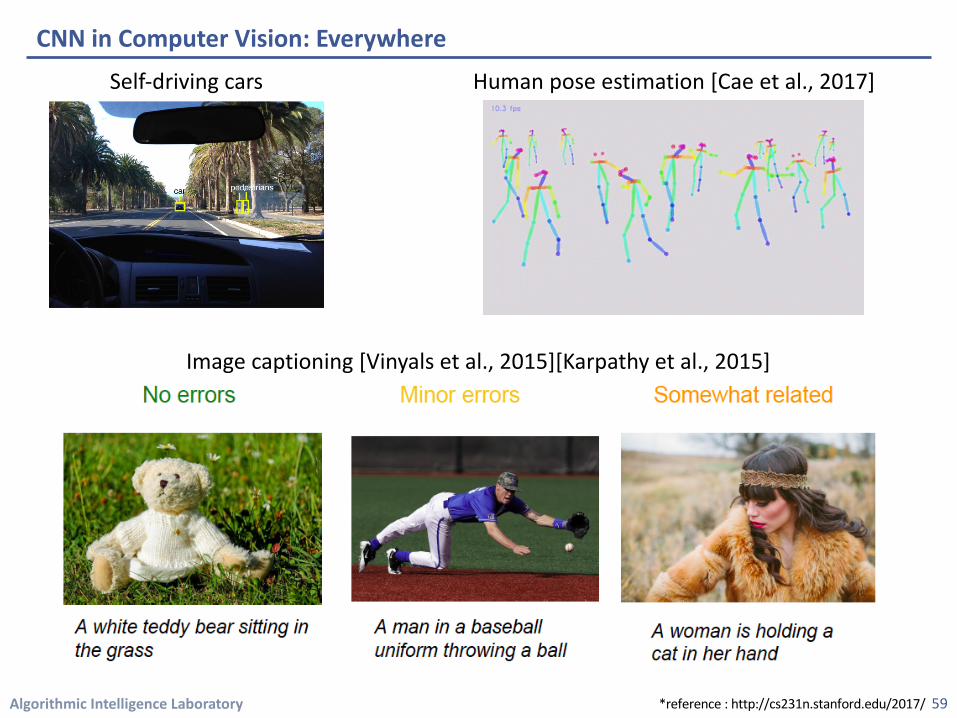
CNN in Computer Vision: Everywhere
59
Self-driving cars Human pose estimation [Cae et al., 2017]
Image captioning [Vinyals et al., 2015][Karpathy et al., 2015]
*reference : http://cs231n.stanford.edu/2017/
Algorithmic Intelligence Laboratory
1. Deep Neural Networks (DNN)• Basics • Training : Back propagation
2. Convolutional Neural Networks (CNN)• Basics• Convolution and Pooling• Some applications
3. Recurrent Neural Networks (RNN)• Basics• Character-level language model (example)
4. Question• Why is it difficult to train a deep neural network ?
Table of Contents
60
Algorithmic Intelligence Laboratory
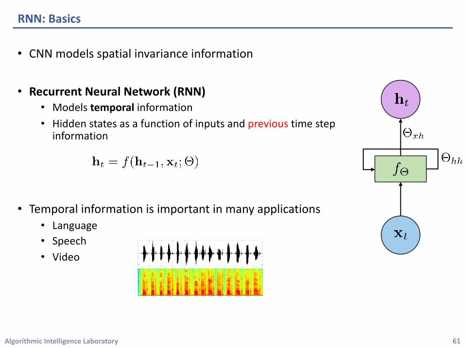
• CNN models spatial invariance information
• Recurrent Neural Network (RNN)• Models temporal information• Hidden states as a function of inputs and previous time step
information
• Temporal information is important in many applications• Language• Speech• Video
RNN: Basics
61
Algorithmic Intelligence Laboratory
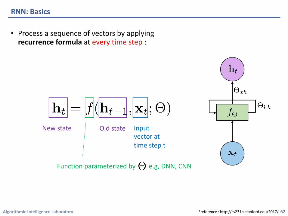
• Process a sequence of vectors by applying recurrence formula at every time step :
RNN: Basics
62
New state Old state Input vector at time step t
Function parameterized by e.g, DNN, CNN
*reference : http://cs231n.stanford.edu/2017/
Algorithmic Intelligence Laboratory
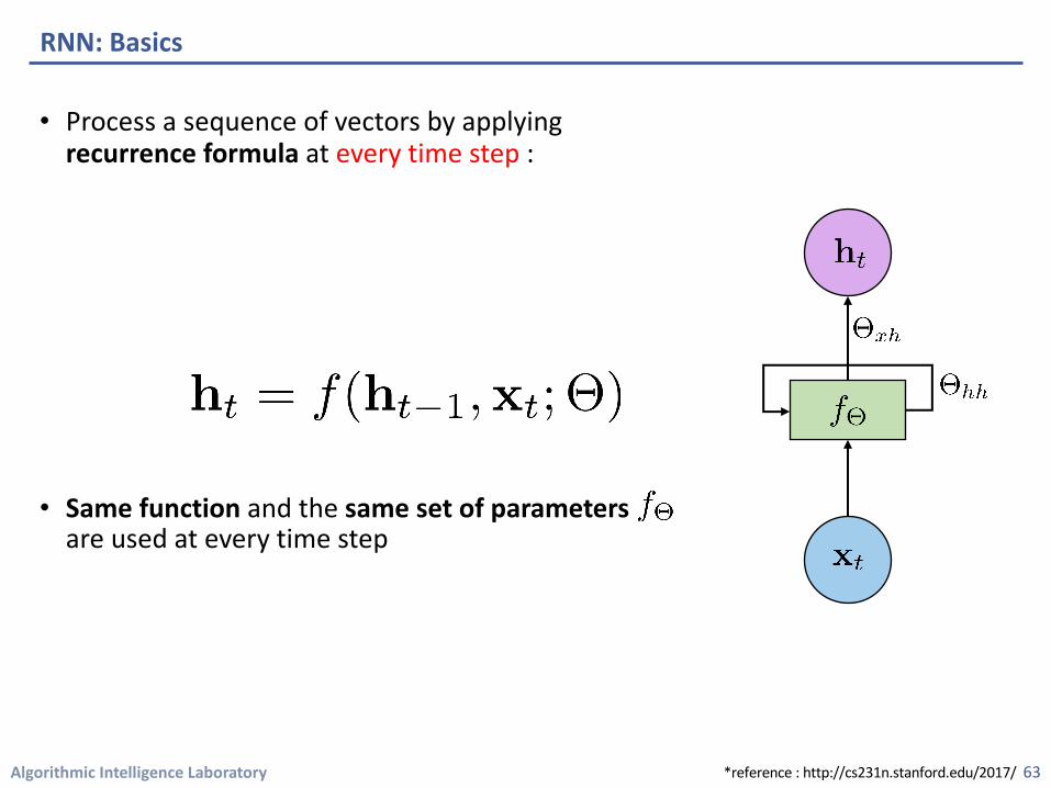
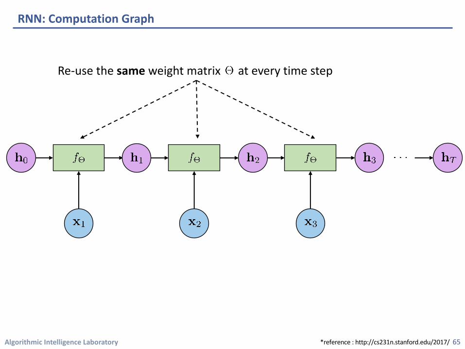
• Process a sequence of vectors by applying recurrence formula at every time step :
• Same function and the same set of parameters are used at every time step
RNN: Basics
63*reference : http://cs231n.stanford.edu/2017/
Algorithmic Intelligence Laboratory
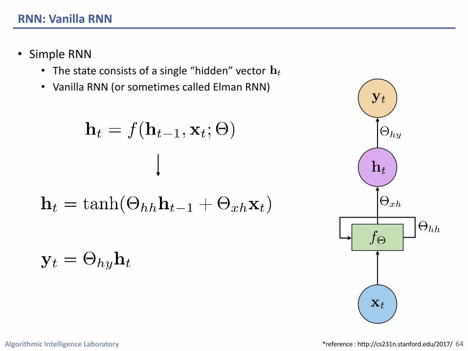
• Simple RNN • The state consists of a single “hidden” vector • Vanilla RNN (or sometimes called Elman RNN)
RNN: Vanilla RNN
64*reference : http://cs231n.stanford.edu/2017/
Algorithmic Intelligence Laboratory
RNN: Computation Graph
65
Re-use the same weight matrix at every time step
*reference : http://cs231n.stanford.edu/2017/
Algorithmic Intelligence Laboratory
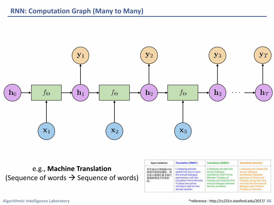
RNN: Computation Graph (Many to Many)
66
e.g., Machine Translation(Sequence of words à Sequence of words)
*reference : http://cs231n.stanford.edu/2017/
Algorithmic Intelligence Laboratory
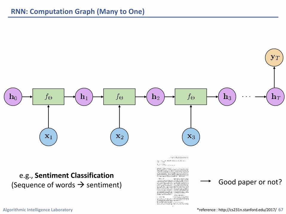
RNN: Computation Graph (Many to One)
67
e.g., Sentiment Classification(Sequence of words à sentiment)
*reference : http://cs231n.stanford.edu/2017/
Good paper or not?
Algorithmic Intelligence Laboratory
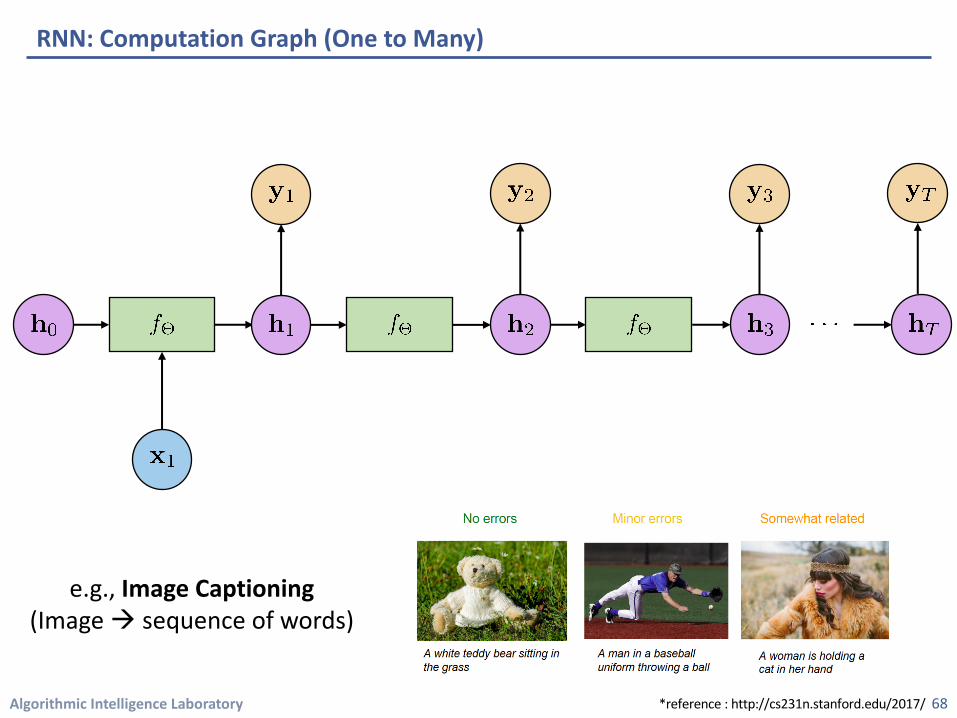
RNN: Computation Graph (One to Many)
68
e.g., Image Captioning(Image à sequence of words)
*reference : http://cs231n.stanford.edu/2017/
Algorithmic Intelligence Laboratory
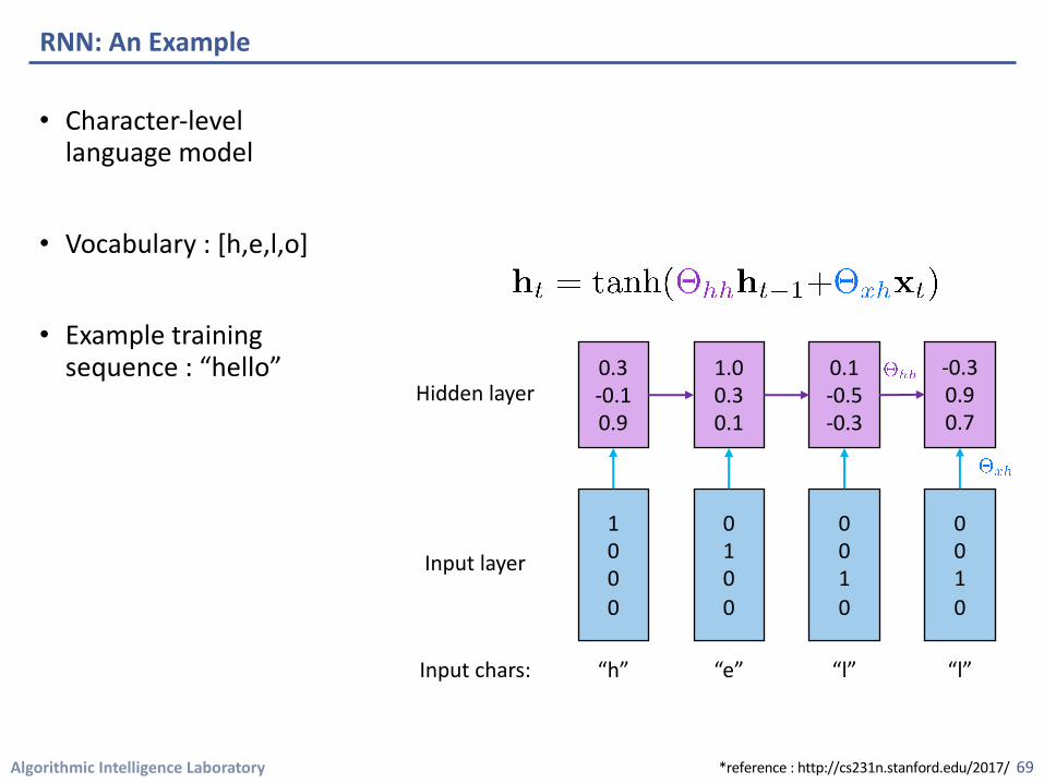
• Character-level language model
• Vocabulary : [h,e,l,o]
• Example training sequence : “hello”
RNN: An Example
69
1000
0100
0010
0010
Input chars:
Input layer
“h” “e” “l” “l”
0.3-0.10.9
1.00.30.1
0.1-0.5-0.3
-0.30.90.7
Hidden layer
*reference : http://cs231n.stanford.edu/2017/
Algorithmic Intelligence Laboratory
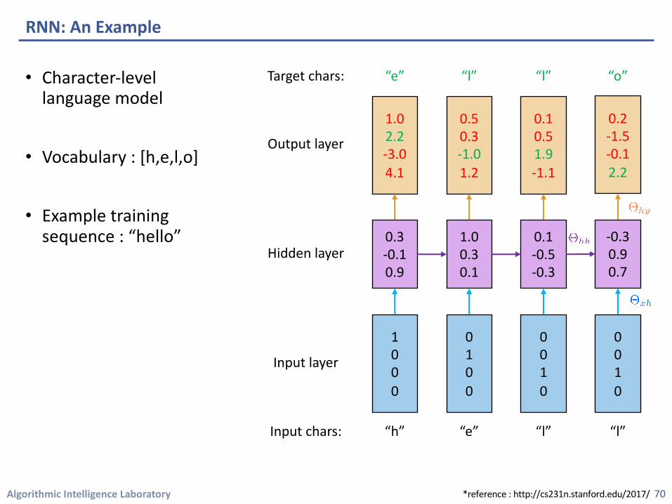
• Character-level language model
• Vocabulary : [h,e,l,o]
• Example training sequence : “hello”
RNN: An Example
70
1.02.2-3.04.1
0.50.3-1.01.2
0.10.51.9-1.1
0.2-1.5-0.12.2
Output layer
Target chars: “e” “l” “l” “o”
1000
0100
0010
0010
Input chars:
Input layer
“h” “e” “l” “l”
0.3-0.10.9
1.00.30.1
0.1-0.5-0.3
-0.30.90.7
Hidden layer
*reference : http://cs231n.stanford.edu/2017/
Algorithmic Intelligence Laboratory
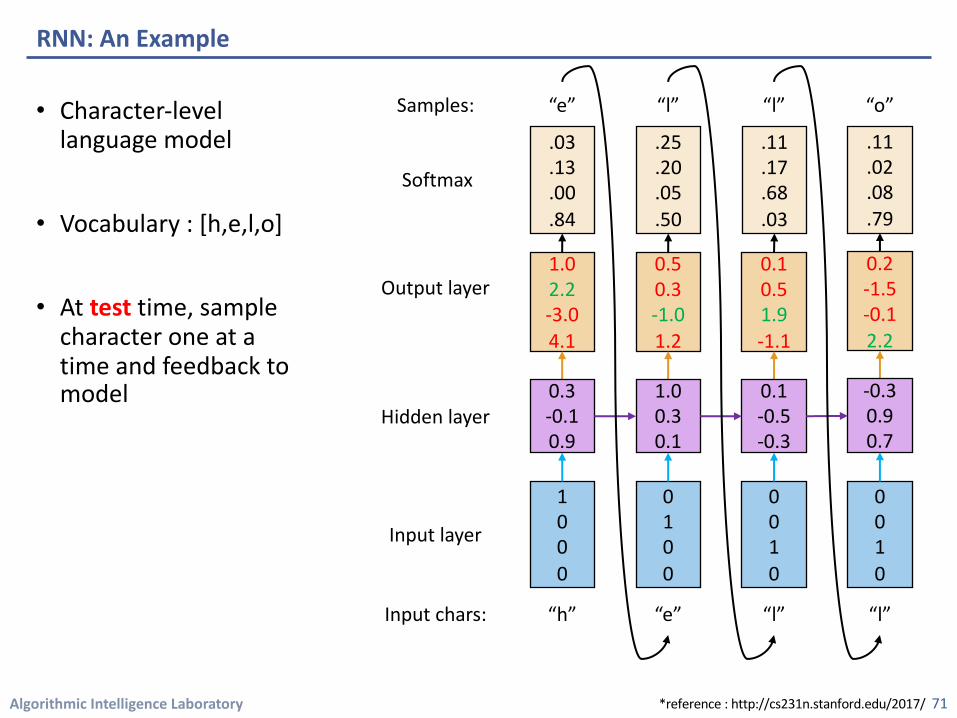
• Character-level language model
• Vocabulary : [h,e,l,o]
• At test time, sample character one at a time and feedback to model
RNN: An Example
71
1.02.2-3.04.1
Output layer
Samples: “e”
1000
Input chars:
Input layer
“h”
0.3-0.10.9
Hidden layer
.03
.13
.00
.84
Softmax
0.50.3-1.01.2
“l”
0100
“e”
1.00.30.1
.25
.20
.05
.50
0.10.51.9-1.1
“l”
0010
“l”
0.1-0.5-0.3
.11
.17
.68
.03
0.2-1.5-0.12.2
“o”
0010
“l”
-0.30.90.7
.11
.02
.08
.79
*reference : http://cs231n.stanford.edu/2017/
Algorithmic Intelligence Laboratory
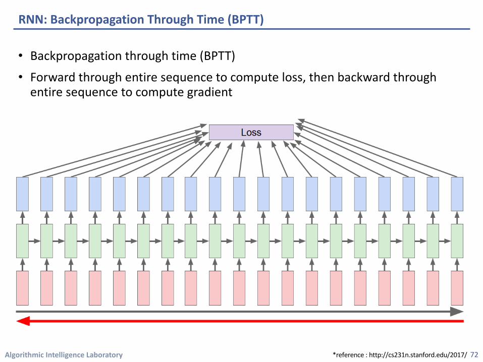
• Backpropagation through time (BPTT)
• Forward through entire sequence to compute loss, then backward through entire sequence to compute gradient
RNN: Backpropagation Through Time (BPTT)
72*reference : http://cs231n.stanford.edu/2017/
Algorithmic Intelligence Laboratory
1. Deep Neural Networks (DNN)• Basics • Training : Back propagation
2. Convolutional Neural Networks (CNN)• Basics• Convolution and Pooling• Some applications
3. Recurrent Neural Networks (RNN)• Basics• Character-level language model (example)
4. Question• Why is it difficult to train a deep neural network?
Contents
73
Algorithmic Intelligence Laboratory
• Why is it difficult to train a deep neural network?
• Can we just simply stack multiple layers and train them all? • Unfortunately, it does not work well • Even if we have infinite amount of computational resource
Vanishing gradient problem :• The magnitude of the gradients shrink exponentially as we backpropagate through
many layers• Since typical activation functions such as sigmoid or tanh are bounded• The phenomenon is called vanishing gradient problem
Question
74
Algorithmic Intelligence Laboratory
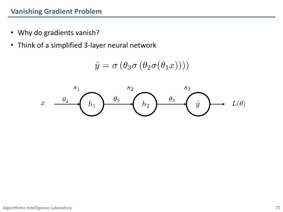
• Why do gradients vanish?
• Think of a simplified 3-layer neural network
Vanishing Gradient Problem
75
Algorithmic Intelligence Laboratory
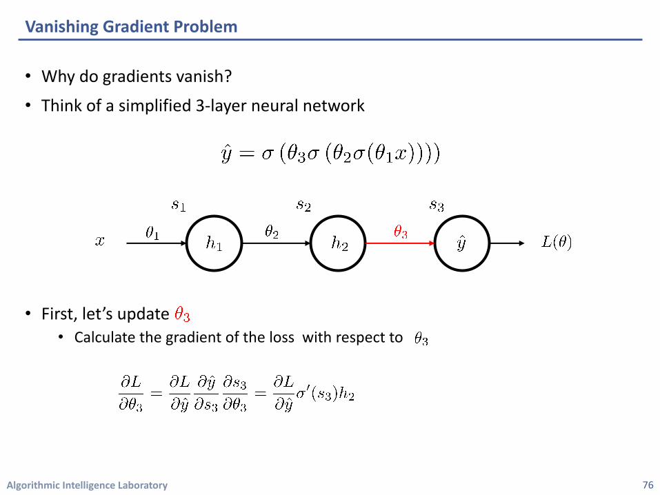
• Why do gradients vanish?
• Think of a simplified 3-layer neural network
• First, let’s update• Calculate the gradient of the loss with respect to
Vanishing Gradient Problem
76
Algorithmic Intelligence Laboratory
Vanishing Gradient Problem
77
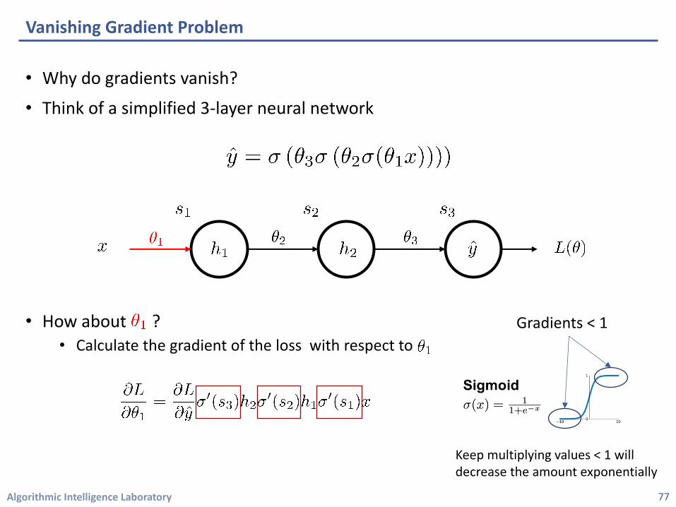
Keep multiplying values < 1 will decrease the amount exponentially
Gradients < 1
• Why do gradients vanish?
• Think of a simplified 3-layer neural network
• How about ?• Calculate the gradient of the loss with respect to
Algorithmic Intelligence Laboratory
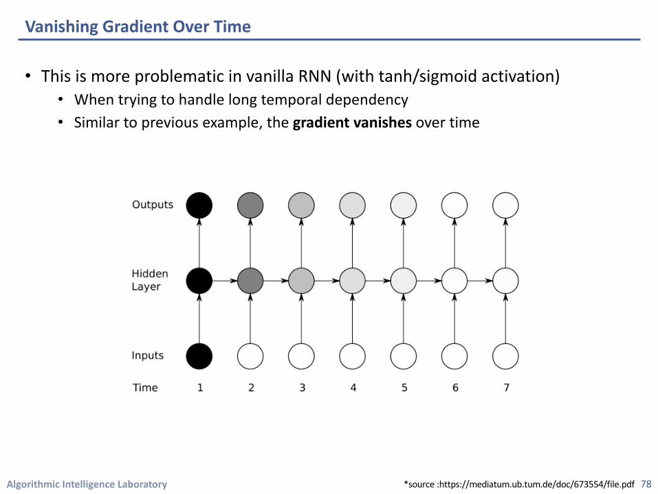
• This is more problematic in vanilla RNN (with tanh/sigmoid activation)• When trying to handle long temporal dependency • Similar to previous example, the gradient vanishes over time
Vanishing Gradient Over Time
78*source :https://mediatum.ub.tum.de/doc/673554/file.pdf
Algorithmic Intelligence Laboratory
• Vanishing gradient problem is critical in training neural network
• Q: Can we just use activation function that has gradients > 1?
Quiz
79
Algorithmic Intelligence Laboratory
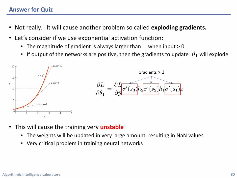
• Not really. It will cause another problem so called exploding gradients.
• Let’s consider if we use exponential activation function:• The magnitude of gradient is always larger than 1 when input > 0 • If output of the networks are positive, then the gradients to update will explode
• This will cause the training very unstable • The weights will be updated in very large amount, resulting in NaN values • Very critical problem in training neural networks
Answer for Quiz
80
Gradients > 1
Algorithmic Intelligence Laboratory
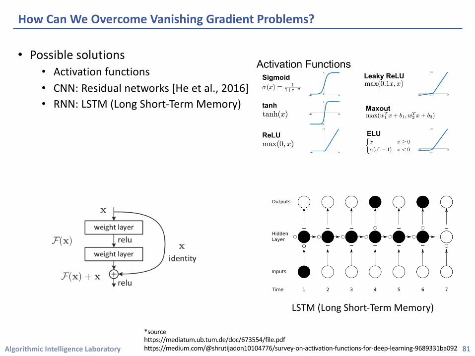
• Possible solutions • Activation functions • CNN: Residual networks [He et al., 2016] • RNN: LSTM (Long Short-Term Memory)
How Can We Overcome Vanishing Gradient Problems?
81
LSTM (Long Short-Term Memory)
*sourcehttps://mediatum.ub.tum.de/doc/673554/file.pdfhttps://medium.com/@shrutijadon10104776/survey-on-activation-functions-for-deep-learning-9689331ba092
Algorithmic Intelligence Laboratory
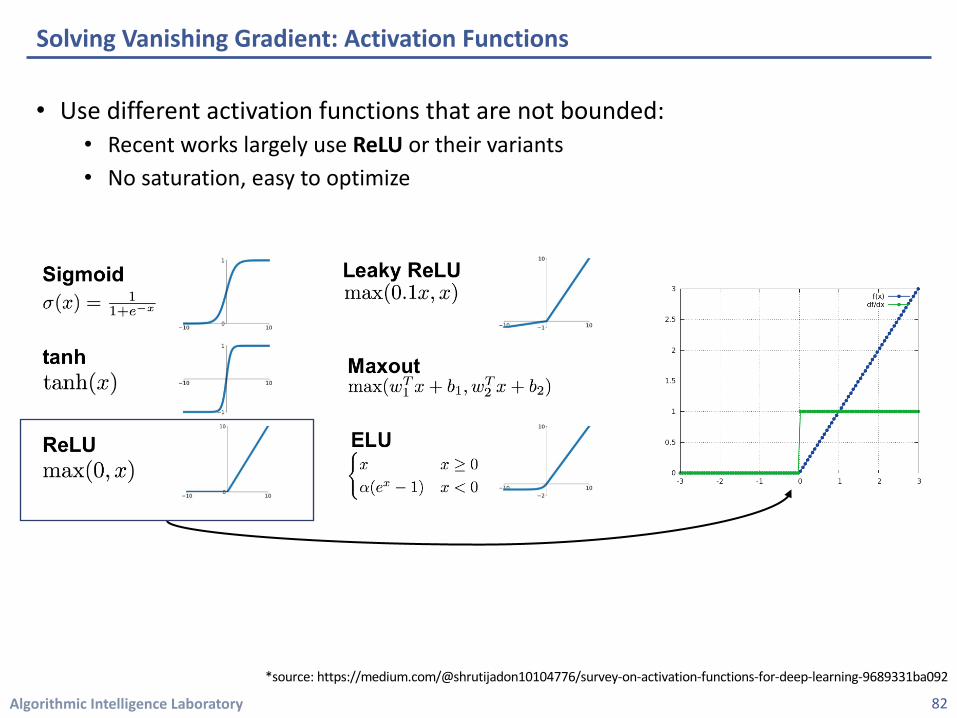
• Use different activation functions that are not bounded: • Recent works largely use ReLU or their variants • No saturation, easy to optimize
Solving Vanishing Gradient: Activation Functions
82
*source: https://medium.com/@shrutijadon10104776/survey-on-activation-functions-for-deep-learning-9689331ba092
Algorithmic Intelligence Laboratory
Solving Vanishing Gradient: Activation Functions
83
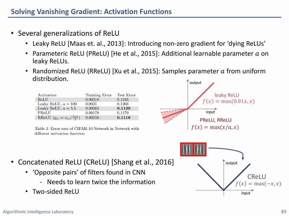
• Several generalizations of ReLU• Leaky ReLU [Maas et. al., 2013]: Introducing non-zero gradient for ‘dying ReLUs’ • Parameteric ReLU (PReLU) [He et al., 2015]: Additional learnable parameter 𝑎 on
leaky ReLUs.• Randomized ReLU (RReLU) [Xu et al., 2015]: Samples parameter 𝑎 from uniform
distribution.
• Concatenated ReLU (CReLU) [Shang et al., 2016]• ‘Opposite pairs’ of filters found in CNN
- Needs to learn twice the information• Two-sided ReLU
input
output
PReLU, RReLU𝑓 𝑥 = max(𝑥/𝑎, 𝑥)
leaky ReLU𝑓 𝑥 = max(0.01𝑥, 𝑥)
CReLU
input
output
𝑓 𝑥 = max(−𝑥, 𝑥)
Algorithmic Intelligence Laboratory
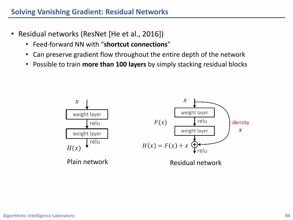
• Residual networks (ResNet [He et al., 2016])• Feed-forward NN with “shortcut connections”• Can preserve gradient flow throughout the entire depth of the network • Possible to train more than 100 layers by simply stacking residual blocks
Solving Vanishing Gradient: Residual Networks
84
Plain network Residual network
Algorithmic Intelligence Laboratory
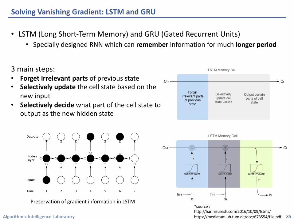
• LSTM (Long Short-Term Memory) and GRU (Gated Recurrent Units)• Specially designed RNN which can remember information for much longer period
Solving Vanishing Gradient: LSTM and GRU
85
Preservation of gradient information in LSTM
3 main steps:• Forget irrelevant parts of previous state• Selectively update the cell state based on the
new input • Selectively decide what part of the cell state to
output as the new hidden state
*source : http://harinisuresh.com/2016/10/09/lstms/https://mediatum.ub.tum.de/doc/673554/file.pdf
Algorithmic Intelligence Laboratory
• [Nair et al., 2010] "Rectified linear units improve restricted boltzmann machines." ICML 2010.link : https://dl.acm.org/citation.cfm?id=3104425
• [Krizhevsky et al., 2012] "Imagenet classification with deep convolutional neural networks." NIPS 2012link : https://papers.nips.cc/paper/4824-imagenet-classification-with-deep-convolutional-neural-networks.pdf
• [Maas et al., 2013] "Rectifier nonlinearities improve neural network acoustic models." ICML 2013.link : https://ai.stanford.edu/~amaas/papers/relu_hybrid_icml2013_final.pdf
• [Farabet et al., 2013] "Learning hierarchical features for scene labeling." IEEE transactions on PAMI 2013link : https://www.ncbi.nlm.nih.gov/pubmed/23787344
• [Zeiler et al., 2014] "Visualizing and understanding convolutional networks." ECCV 2014.link : https://cs.nyu.edu/~fergus/papers/zeilerECCV2014.pdf
• [Simonyan et al., 2015] "Very deep convolutional networks for large-scale image recognition.” ICLR 2015link : https://arxiv.org/abs/1409.1556
• [Ren et al., 2015] "Faster r-cnn: Towards real-time object detection with region proposal networks." NIPS 2015link : https://arxiv.org/abs/1506.01497
• [Vinyals et al., 2015] "Show and tell: A neural image caption generator." CVPR 2015.link : https://arxiv.org/abs/1411.4555
• [Karpathy et al., 2015] "Deep visual-semantic alignments for generating image descriptions." CVPR 2015link : https://cs.stanford.edu/people/karpathy/cvpr2015.pdf
• [He et al., 2015] "Delving deep into rectifiers: Surpassing human-level performance on imagenetclassification." ICCV 2015.link : https://arxiv.org/abs/1502.01852
References
86
Algorithmic Intelligence Laboratory
• [Xu et al., 2015] "Empirical evaluation of rectified activations in convolutional network." arXiv preprint, 2015.link : https://arxiv.org/abs/1505.00853
• [Shang et al., 2016] "Understanding and improving convolutional neural networks via concatenated rectified linear units." ICML 2016.link : https://arxiv.org/abs/1603.05201
• [He et al., 2016] "Deep residual learning for image recognition." CVPR 2016link : https://arxiv.org/abs/1512.03385
• [Cae et al., 2017] "Realtime multi-person 2d pose estimation using part affinity fields.", CVPR 2017link : https://arxiv.org/abs/1611.08050
• [Fei-Fei and Karpathy, 2017] “CS231n: Convolutional Neural Networks for Visual Recognition”, 2017. (Stanford University)link : http://cs231n.stanford.edu/2017/
References
87


![Comprehensive Overview on Computational Intelligence ......bearing fault diagnosis. Jia, et al [32], used DNN for intelligence fault diagnosis in rotating machinery, espe-cially in](https://img.pdfslide.us/doc/110x75/611e61b8cf84b46d480b7ec6/comprehensive-overview-on-computational-intelligence-bearing-fault-diagnosis.jpg)