Introduction to Neural Networks...Introduction to Neural Networks Steve Renals Automatic Speech Recognition { ASR Lecture 7 9 February 2017 ASR Lecture 7 Introduction to Neural Networks1

Introduction to Neural Networks

Steve Renals

Automatic Speech Recognition – ASR Lecture 79 February 2017

ASR Lecture 7 Introduction to Neural Networks 1

Local Phonetic Scores and Sequence Modelling

DTW - local distances (Euclidean)

HMM - emission probabilities (Gaussian or GMM)

x1

S0

2

3

1

4

S

S

S

S

aa

a

a

a

a

01

12

2322

33 34

a11

764321 time5

x x3

x4

x5

x6

x72

observations

states

Compute the phonetic score(acoustic-frame, phone-model) –this does the detailed matching at the frame-level

Chain phonetic scores together in a sequence - DTW, HMM


Phonetic scores

Task: given an input acoustic frame, output a score for each phone

X(t)

/aa/ .01

/ae/ .03

/ax/ .01

/ao/ .04

/b/ .09

/ch/ .67

/d/ .06

…

/zh/ .15

Acoustic frame(at time t)

Phonetic Scores(at time t)

f(t)


Phonetic scores

Compute the phonetic scores using a single layer neural network

/aa/ .01

/ae/ .03

/ax/ .01

/ao/ .04

/b/ .09

/ch/ .67

/d/ .06

…

/zh/ .15

/aa/ .01

/ae/ .03

/ax/ .01

/ao/ .04

/b/ .09

/ch/ .67

/d/ .06

…

/zh/ .15

Acoustic frame(at time t)

X(t)


f(t)

/aa/ .01

/ae/ .03

/ax/ .01

/ao/ .04

/b/ .09

/ch/ .67

/d/ .06

…

/zh/ .15

0.33

-0.23

0.71

0.47

0.11

-0.32

-0.02

…

0.22

w7(/aa/)

w1(/aa/)

w2(/aa/)

w3(/aa/)

w4(/aa/)

w5(/aa/)

w6(/aa/)

wd(/aa/)

Each output computes its scoreas a weighted sum of the current inputs

…


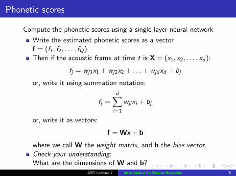
Phonetic scores

Compute the phonetic scores using a single layer neural network

Write the estimated phonetic scores as a vectorf = (f1, f2, . . . , fQ)

Then if the acoustic frame at time t is X = (x1, x2, . . . , xd):

fj = wj1x1 + wj2x2 + . . .+ wjdxd + bj

or, write it using summation notation:

fj =d∑

i=1

wjixi + bj

or, write it as vectors:

f = Wx + b

where we call W the weight matrix, and b the bias vector.

Check your understanding:What are the dimensions of W and b?


Error function

f(t) = Wx(t) + b

observed

trained

estimated

How do we learn the parameters W and b?

Minimise an Error Function: Define a function which is 0when the output f(n) equals the target output r(n) for all nTarget output: for TIMIT the target output corresponds tothe phone label for each frameMean square error: define the error function E as the meansquare difference between output and the target:

E =1

2· 1

N

N∑

n=1

||f(n)− r(n)||2

where there are N frames of training data in totalASR Lecture 7 Introduction to Neural Networks 6

Notes on the error function

f is a function of the acoustic data x and the weights andbiases of the network (W and b)

This means that as well as depending on the training data (xand r), E is also a function of the weights and biases, since itis a function of f

We want to minimise the error function given a fixed trainingset: we must set W and b to minimise E

Weight space: given the training set we can imagine a spacewhere every possible value of W and b results in a specificvalue of E . We want to find the minimum of E in this weightspace.

Gradient descent: find the minimum iteratively – given acurrent point in weight space find the direction of steepestdescent, and change W and b to move in that direction


Gradient Descent

Iterative update – after seeing some training data, we adjustthe weights and biases to reduce the error. Repeat untilconvergence.

To update a parameter so as to reduce the error, we movedownhill in the direction of steepest descent. Thus to train anetwork we must compute the gradient of the error withrespect to the weights and biases:

∂E∂w10

· ∂E∂w1i

· ∂E∂w1d

. . .∂E∂wj0

· ∂E∂wji

· ∂E∂wjd

. . .∂E∂wQ0

· ∂E∂wQi

· ∂E∂wQd

(∂E∂b1

· ∂E∂bj

· ∂E∂bQ

)


Gradient Descent Procedure

1 Initialise weights and biases with small random numbers2 For each batch of training data

1 Initialise total gradients: ∆wki = 0, ∆bk = 02 For each training example n in the batch:

Compute the error E n

For all k, i : Compute the gradients ∂E n/∂wki , ∂En/∂bk

Update the total gradients by accumulating the gradients forexample n

∆wki ← ∆wki +∂E n

∂wki∀k, i

∆bk ← ∆bk +∂E n

∂bk∀k

3 Update weights:

wki ← wki − η∆wki ∀k , ibk ← bk − η∆bk ∀k

Terminate either after a fixed number of epochs, or when the errorstops decreasing by more than a threshold.


Gradient in SLN

How do we compute the gradients ∂En

∂wkiand ∂En

∂bk?

En =1

2

K∑

k=1

(f nk − rnk )2 =1

2

K∑

k=1

(d∑

i=1

(wkixni + bk)− rnk

)2

∂En

∂wki= (f nk − rnk )xni = δnkx

ni δnk = f nk − rnk

The delta rule: gradient of the error with respect to a weight wki

is the product of the error (delta) at the output of the weight (rk)multiplied by the value of the unit at the input to the weight (xi ).

Check your understanding: Show that

∂En

∂bk= δnk


Applying gradient descent to a single-layer network

x1 x2 x3 x4 x5

f2 =5X

i=1

w2ixi

w24

�w24 =X

n

(fn2 � rn

2 )xn4


Acoustic context

Use multiple frames of acoustic context

/aa/ .01

/ae/ .03

/ax/ .01

/ao/ .04

/b/ .09

/ch/ .67

/d/ .06

…

/zh/ .15

/aa/ .11

/ae/ .09

/ax/ .04

/ao/ .04

/b/ .01

…

/i/ .65

…

/zh/ .01

Acoustic inputX(t) with +/-3

frames of context


f(t)

/aa/ .01X(t-3)

X(t-2)

X(t-1)

X(t)

X(t+1)

X(t+2)

X(t+3)


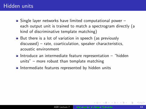
Hidden units

Single layer networks have limited computational power –each output unit is trained to match a spectrogram directly (akind of discriminative template matching)

But there is a lot of variation in speech (as previouslydiscussed) – rate, coarticulation, speaker characteristics,acoustic environment

Introduce an intermediate feature representation – “hiddenunits” – more robust than template matching

Intermediate features represented by hidden units


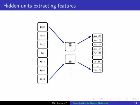
Hidden units extracting features

/aa/ .01

/ae/ .03

/ax/ .01

/ao/ .04

/b/ .09

/ch/ .67

/d/ .06

…

/zh/ .15

/aa/ .11

/ae/ .09

/ax/ .04

/ao/ .04

/b/ .01

…

/i/ .65

…

/zh/ .01

/aa/ .01X(t-3)

X(t-2)

X(t-1)

X(t)

X(t+1)

X(t+2)

X(t+3)

.

.

.

.

.

.


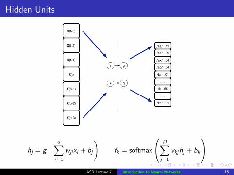
Hidden Units

/aa/ .01

/ae/ .03

/ax/ .01

/ao/ .04

/b/ .09

/ch/ .67

/d/ .06

…

/zh/ .15

/aa/ .11

/ae/ .09

/ax/ .04

/ao/ .04

/b/ .01

…

/i/ .65

…

/zh/ .01

/aa/ .01X(t-3)

X(t-2)

X(t-1)

X(t)

X(t+1)

X(t+2)

X(t+3)

.

.

.

.

.

.

+

+

g

g

hj = g

(d∑

i=1

wjixi + bj

)fk = softmax

H∑

j=1

vkjhj + bk


Sigmoid function

−5 −4 −3 −2 −1 0 1 2 3 4 50

0.1

0.2

0.3

0.4

0.5

0.6

0.7

0.8

0.9

1

a

g(a)

Logistic sigmoid activation function g(a) = 1/(1+exp(−a))


Softmax

yk =exp(ak)

∑Kj=1 exp(aj)

ak =H∑

j=1

vkjhj + bk

This form of activation has the following properties

Each output will be between 0 and 1The denominator ensures that the K outputs will sum to 1

Using softmax we can interpret the network output ynk as anestimate of P(k|xn)


Cross-entropy error function

Cross-entropy error function:

En = −C∑

k=1

rnk ln f nk

Optimise the weights W to maximise the log probability – orto minimise the negative log probability.

A neat thing about softmax: if we train with cross-entropyerror function, we get a simple form for the gradients of theoutput weights:

∂En

∂vkj= (fk − rk)︸︷︷︸

δk

hj


Training multilayered networks – output layer

softmax

g

Outputs softmax

Hidden units

softmax

xi

hj

f1 f` fK

v1j v`j

vKj

wji


Training multilayered networks – output layer

softmax

g

Outputs softmax

Hidden units

softmax

xi

hj

f1 f` fK

�K�`�1

v1j v`j

vKj

wji

@E

@vkj= �khj


Backprop

Hidden units make training the weights more complicated,since the hidden units affect the error function indirectly viaall the outputs

The Credit assignment problem: what is the “error” of ahidden unit? how important is input-hidden weight wji tooutput unit k?

Solution: back-propagate the deltas through the network

δj for a hidden unit is the weighted sum of the deltas of theconnected output units. (Propagate the δ values backwardsthrough the network)

Backprop provides way of estimating the error of each hiddenunit


Backprop

softmax

g

Outputs softmax

Hidden units

softmax

xi

hj

f1 f` fK

�K�`�1

v1j v`j

vKj

�j =

X

`

�lv`j

!g0

@E

@wji= �jxi

wji

@E

@vkj= �khj


Back-propagation of error

The back-propagation of error algorithm is summarised asfollows:

1 Apply an input vectors from the training set, x, to the networkand forward propagate to obtain the output vector f

2 Using the target vector r compute the error E n

3 Evaluate the error signals δk for each output unit4 Evaluate the error signals δj for each hidden unit using

back-propagation of error5 Evaluate the derivatives for each training pattern

Back-propagation can be extended to multiple hidden layers,in each case computing the δs for the current layer as aweighted sum of the δs of the next layer


Summary and Reading

Single-layer and multi-layer neural networks

Error functions, weight space and gradient descent training

Multilayer networks and back-propagation

Transfer functions – sigmoid and softmax

Acoustic context

M Nielsen, Neural Networks and Deep Learning,http://neuralnetworksanddeeplearning.com (chapters1, 2, and 3)

Next lecture: Neural network acoustic models


http://neuralnetworksanddeeplearning.com

Documents

Introduction to Neural Networks...Introduction to Neural Networks Steve Renals Automatic Speech Recognition { ASR Lecture 7 9 February 2017 ASR Lecture 7 Introduction to Neural Networks1