Embed Size (px)
Citation preview
1
Path and Motion Planning
Introduction to Mobile Robotics
Wolfram Burgard, Diego Tipaldi, Barbara Frank

2
Motion Planning
Latombe (1991):
“…eminently necessary since, by definition, a
robot accomplishes tasks by moving in the real
world.”
Goals:
Collision-free trajectories.
Robot should reach the goal location as fast as possible.

3
… in Dynamic Environments
How to react to unforeseen obstacles?
efficiency
reliability
Dynamic Window Approaches [Simmons, 96], [Fox et al., 97], [Brock & Khatib, 99]
Grid map based planning [Konolige, 00]
Nearness Diagram Navigation [Minguez at al., 2001, 2002]
Vector-Field-Histogram+ [Ulrich & Borenstein, 98]
A*, D*, D* Lite, ARA*, …

4
Two Challenges
Calculate the optimal path taking potential uncertainties in the actions into account
Quickly generate actions in the case of unforeseen objects
5
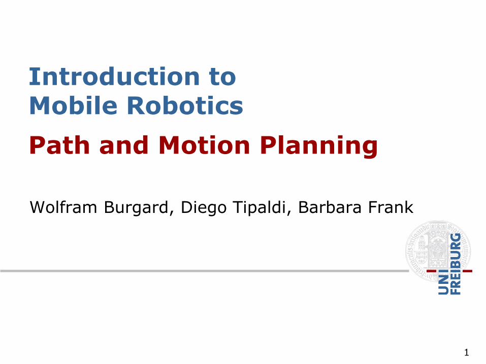
Classic Two-layered Architecture
Planning
Collision Avoidance
sensor data
map
robot
low frequency
high frequency
sub-goal
motion command

6
Dynamic Window Approach
Collision avoidance: Determine collision-free trajectories using geometric operations
Here: Robot moves on circular arcs
Motion commands (v,ω)
Which (v,ω) are admissible and reachable?

7
Admissible Velocities
Speeds are admissible if the robot would be able to stop before reaching the obstacle

8
Reachable Velocities
Speeds that are reachable by acceleration

9
DWA Search Space
Vs = all possible speeds of the robot.
Va = obstacle free area.
Vd = speeds reachable within a certain time frame based on possible accelerations.

10
Dynamic Window Approach
How to choose <v,ω>?
Steering commands are chosen by a heuristic navigation function.
This function tries to minimize the travel-time by: “driving fast in the right direction.”
11
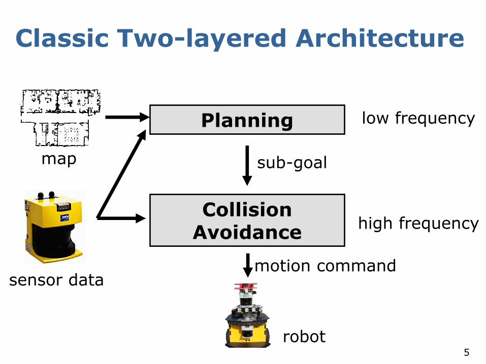
Dynamic Window Approach
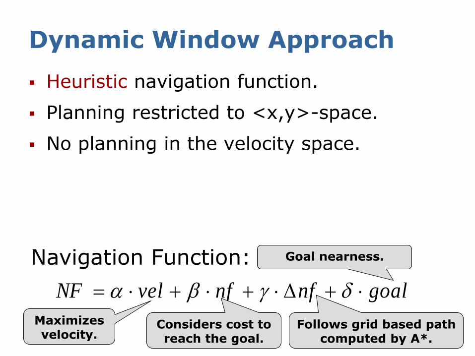
Heuristic navigation function.
Planning restricted to <x,y>-space.
No planning in the velocity space.
goalnfnfvelNF
Navigation Function: [Brock & Khatib, 99]

12
goalnfnfvelNF
Navigation Function: [Brock & Khatib, 99]
Maximizes velocity.
Heuristic navigation function.
Planning restricted to <x,y>-space.
No planning in the velocity space.
Dynamic Window Approach

13
goalnfnfvelNF
Navigation Function: [Brock & Khatib, 99]
Considers cost to reach the goal.
Maximizes velocity.
Heuristic navigation function.
Planning restricted to <x,y>-space.
No planning in the velocity space.
Dynamic Window Approach

14
goalnfnfvelNF
Navigation Function: [Brock & Khatib, 99]
Maximizes velocity.
Considers cost to reach the goal.
Follows grid based path computed by A*.
Heuristic navigation function.
Planning restricted to <x,y>-space.
No planning in the velocity space.
Dynamic Window Approach
15
Navigation Function: [Brock & Khatib, 99] Goal nearness.
Follows grid based path computed by A*.
goalnfnfvelNF
Maximizes velocity.
Considers cost to reach the goal.
Heuristic navigation function.
Planning restricted to <x,y>-space.
No planning in the velocity space.
Dynamic Window Approach
16
Dynamic Window Approach
Reacts quickly.
Low CPU power requirements.
Guides a robot on a collision-free path.
Successfully used in a lot of real-world scenarios.
Resulting trajectories sometimes sub-optimal.
Local minima might prevent the robot from reaching the goal location.

17
Problems of DWAs
goalnfnfvelNF

18
Problems of DWAs
goalnfnfvelNF
Robot‘s velocity.

19
Problems of DWAs
goalnfnfvelNF
Preferred direction of NF.
Robot‘s velocity.

20
Problems of DWAs
goalnfnfvelNF
21
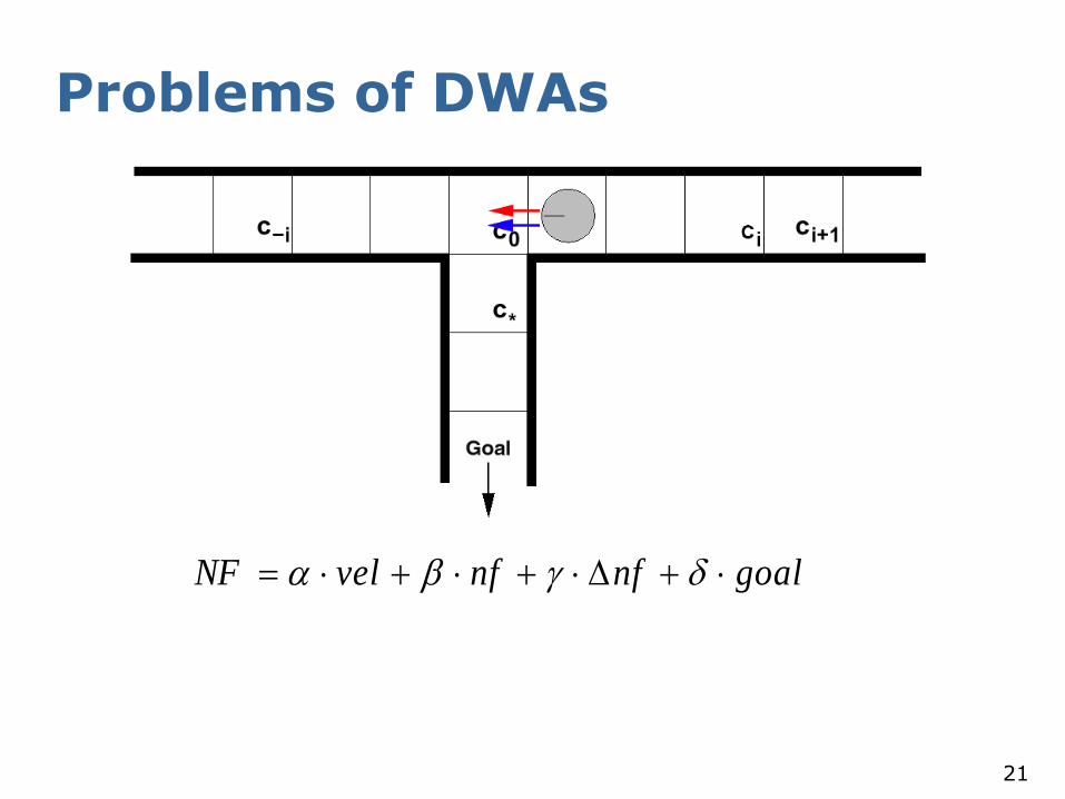
Problems of DWAs
goalnfnfvelNF

22
Problems of DWAs
goalnfnfvelNF
The robot drives too fast at c0 to enter corridor facing south.

23
Problems of DWAs
goalnfnfvelNF

24
Problems of DWAs
goalnfnfvelNF

25
Problems of DWAs
Same situation as in the beginning.
DWAs have problems to reach the goal.

26
Problems of DWAs
Typical problem in a real world situation:
Robot does not slow down early enough to enter the doorway.

Motion Planning Formulation
The problem of motion planning can be stated as follows. Given:
A start pose of the robot
A desired goal pose
A geometric description of the robot
A geometric description of the world
Find a path that moves the robot gradually from start to goal while never touching any obstacle
27

Configuration Space
Although the motion planning problem is defined in the regular world, it lives in another space: the configuration space
A robot configuration q is a specification of
the positions of all robot points relative to a fixed coordinate system
Usually a configuration is expressed as a vector of positions and orientations
28

Configuration Space
Free space and obstacle region
With being the work space, the set of obstacles, the robot in configuration
We further define
: start configuration
: goal configuration
29

Then, motion planning amounts to
Finding a continuous path
with
Given this setting, we can do planning with the robot being a point in C-space!
Configuration Space
30
C-Space Discretizations
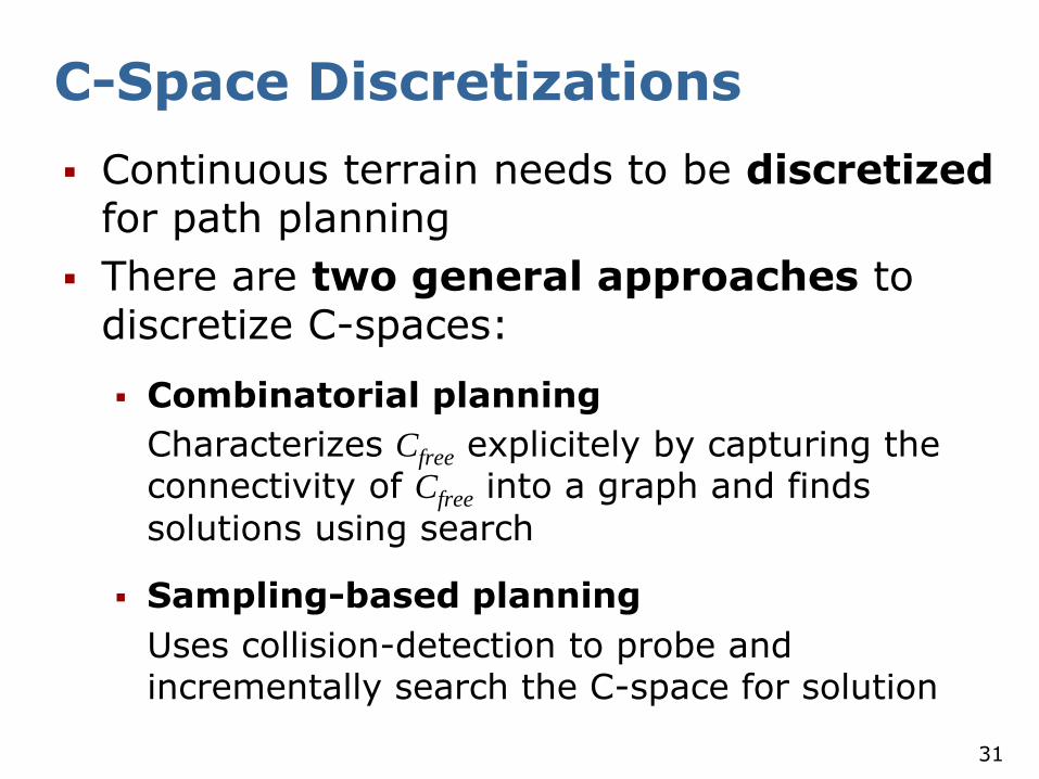
Continuous terrain needs to be discretized for path planning
There are two general approaches to discretize C-spaces:
Combinatorial planning
Characterizes Cfree explicitely by capturing the connectivity of Cfree into a graph and finds
solutions using search
Sampling-based planning
Uses collision-detection to probe and incrementally search the C-space for solution
31

Search
The problem of search: finding a sequence of actions (a path) that leads to desirable states (a goal)
Uninformed search: besides the problem definition, no further information about the domain („blind search“)
The only thing one can do is to expand nodes differently
Example algorithms: breadth-first, uniform-cost, depth-first, bidirectional, etc.
32

Search
The problem of search: finding a sequence of actions (a path) that leads to desirable states (a goal)
Informed search: further information about the domain through heuristics
Capability to say that a node is "more promising" than another node
Example algorithms: greedy best-first search, A*, many variants of A*, D*, etc.
33

Search
The performance of a search algorithm is measured in four ways:
Completeness: does the algorithm find the solution when there is one?
Optimality: is the solution the best one of all possible solutions in terms of path cost?
Time complexity: how long does it take to find a solution?
Space complexity: how much memory is needed to perform the search?
34

Discretized Configuration Space
35

Uninformed Search
Breadth-first
Complete
Optimal if action costs equal
Time and space: O(bd)
Depth-first
Not complete in infinite spaces
Not optimal
Time: O(bm)
Space: O(bm) (can forget
explored subtrees)
(b: branching factor, d: goal depth, m: max. tree depth)
36
37
Informed Search: A*
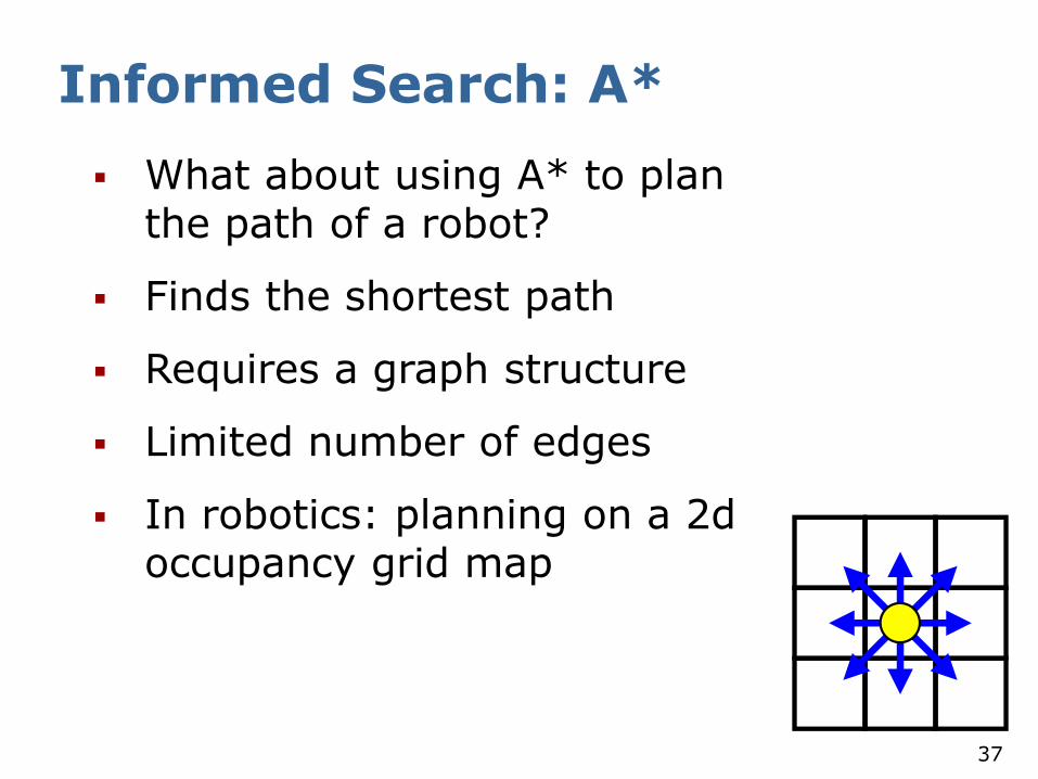
What about using A* to plan the path of a robot?
Finds the shortest path
Requires a graph structure
Limited number of edges
In robotics: planning on a 2d occupancy grid map

38
A*: Minimize the estimated path costs
g(n) = actual cost from the initial state to n.
h(n) = estimated cost from n to the next goal.
f(n) = g(n) + h(n), the estimated cost of the cheapest solution through n.
Let h*(n) be the actual cost of the optimal path from n to the next goal.
h is admissible if the following holds for all n :
h(n) h*(n)
We require that for A*, h is admissible (the straight-line distance is admissible in the Euclidean Space).

39
Example: Path Planning for Robots in a Grid-World

40
Deterministic Value Iteration
To compute the shortest path from every state to one goal state, use (deterministic) value iteration.
Very similar to Dijkstra’s Algorithm.
Such a cost distribution is the optimal heuristic for A*.

41
Typical Assumption in Robotics for A* Path Planning
The robot is assumed to be localized.
The robot computes its path based on an occupancy grid.
The correct motion commands are executed.
Is this always true?

42
Problems
What if the robot is slightly delocalized?
Moving on the shortest path guides often the robot on a trajectory close to obstacles.
Trajectory aligned to the grid structure.
43
Convolution of the Grid Map
Convolution blurs the map.
Obstacles are assumed to be bigger than in reality.
Perform an A* search in such a convolved map.
Robot increases distance to obstacles and moves on a short path!

44
Example: Map Convolution
1-d environment, cells c0, …, c5
Cells before and after 2 convolution runs.

45
Convolution
Consider an occupancy map. Than the convolution is defined as:
This is done for each row and each column of the map.
“Gaussian blur”

46
A* in Convolved Maps
The costs are a product of path length and occupancy probability of the cells.
Cells with higher probability (e.g., caused by convolution) are avoided by the robot.
Thus, it keeps distance to obstacles.
This technique is fast and quite reliable.

47
5D-Planning – an Alternative to the Two-layered Architecture
Plans in the full <x,y,θ,v,ω>-configuration space using A*.
Considers the robot's kinematic constraints.
Generates a sequence of steering commands to reach the goal location.
Maximizes trade-off between driving time and distance to obstacles.

48
The Search Space (1)
What is a state in this space? <x,y,θ,v,ω> = current position and speed of the robot
How does a state transition look like? <x1,y1,θ1,v1,ω1> <x2,y2,θ2,v2,ω2>
with motion command (v2,ω2) and
|v1-v2| < av, |ω1-ω2| < aω. Pose of the Robot is a result of the motion equations.
49
The Search Space (2)
Idea: search in the discretized <x,y,θ,v,ω>-space.
Problem: the search space is too huge to be explored within the time constraints (5+ Hz for online motion plannig).
Solution: restrict the full search space.
50
The Main Steps of the Algorithm
1. Update (static) grid map based on sensory input.
2. Use A* to find a trajectory in the <x,y>-space using the updated grid map.
3. Determine a restricted 5d-configuration space based on step 2.
4. Find a trajectory by planning in the restricted <x,y,θ,v,ω>-space.

51
Updating the Grid Map
The environment is represented as a 2d-occupency grid map.
Convolution of the map increases security distance.
Detected obstacles are added.
Cells discovered free are cleared.
update
52
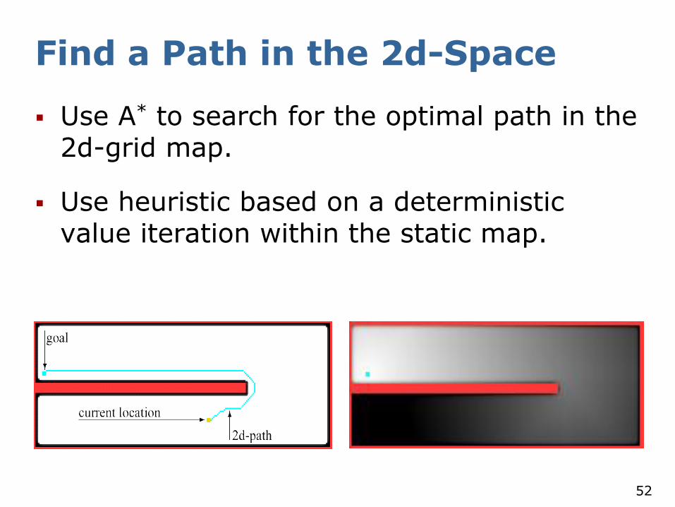
Find a Path in the 2d-Space
Use A* to search for the optimal path in the 2d-grid map.
Use heuristic based on a deterministic value iteration within the static map.

53
Restricting the Search Space
Assumption: the projection of the 5d-path onto the <x,y>-space lies close to the optimal 2d-path.
Therefore: construct a restricted search space (channel) based on the 2d-path.

54
Space Restriction
Resulting search space =
<x, y, θ, v, ω> with (x,y) Є channel.
Choose a sub-goal lying on the 2d-path within the channel.

55
Find a Path in the 5d-Space
Use A* in the restricted 5d-space to find a sequence of steering commands to reach the sub-goal.
To estimate cell costs: perform a deterministic 2d-value iteration within the channel.

56
Examples

57
Timeouts
Steering a robot online requires to set a new steering command every .25 secs.
Abort search after .25 secs.
How to find an admissible steering command?
58
Alternative Steering Command
Previous trajectory still admissible? OK
If not, drive on the 2d-path or use DWA to find new command.

59
Timeout Avoidance
Reduce the size of the channel if the 2d-path has high cost.

60
Example
Robot Albert Planning state

61
Comparison to the DWA (1)
DWAs often have problems entering narrow passages.
DWA planned path. 5D approach.

62
Comparison to the DWA (1)
DWAs often have problems entering narrow passages.
DWA planned path. 5D approach.

63
Comparison to the DWA (2)
The presented approach results in significantly faster motion when driving through narrow passages!

64
Comparison to the Optimum
Channel: with length=5m, width=1.1m
Resulting actions are close to the optimal solution.
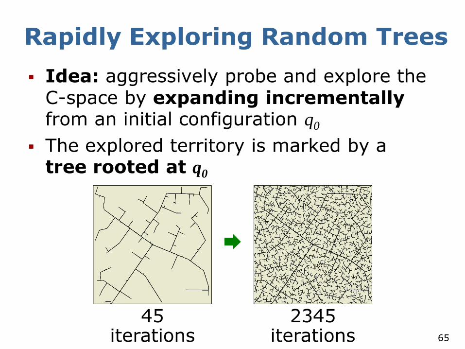
Rapidly Exploring Random Trees
Idea: aggressively probe and explore the C-space by expanding incrementally from an initial configuration q0
The explored territory is marked by a tree rooted at q0
65
45 iterations
2345 iterations

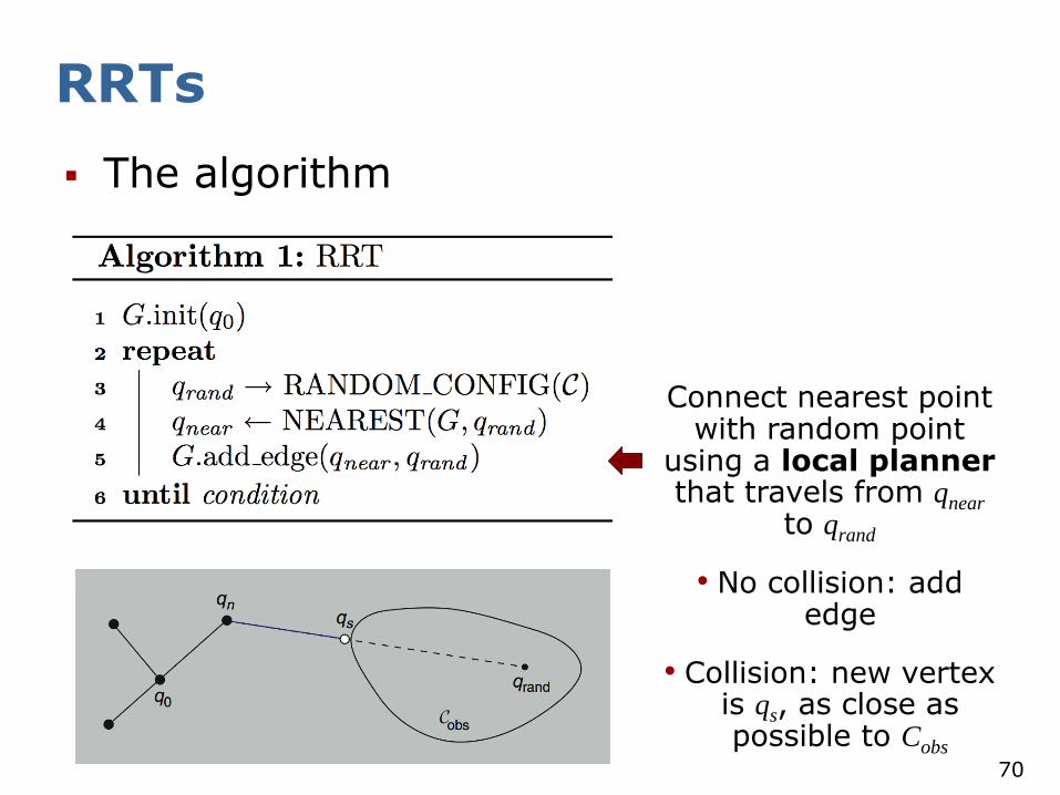
RRTs
The algorithm: Given C and q0
66
Sample from a bounded region centered around q0
E.g. an axis-aligned relative random
translation or random rotation

RRTs
The algorithm
67
Finds closest vertex in G using a distance
function
formally a metric defined on C

RRTs
The algorithm
68
Several stategies to find qnear given the closest
vertex on G:
• Take closest vertex
• Check intermediate points at regular
intervals and split edge at qnear

RRTs
The algorithm
69
Connect nearest point with random point
using a local planner that travels from qnear
to qrand
• No collision: add edge
• Collision: new vertex is qi, as close as possible to Cobs
RRTs
The algorithm
70
Connect nearest point with random point
using a local planner that travels from qnear
to qrand
• No collision: add edge
• Collision: new vertex is qs, as close as possible to Cobs

RRTs
How to perform path planning with RRTs?
1. Start RRT at qI
2. At every, say, 100th iteration, force qrand = qG
3. If qG is reached, problem is solved
Why not picking qG every time?
This will fail and waste much effort in running into CObs instead of exploring the
space
71

RRTs
However, some problems require more effective methods: bidirectional search
Grow two RRTs, one from qI, one from qG
In every other step, try to extend each tree towards the newest vertex of the other tree
72
Filling a well
A bug trap

RRTs
RRTs are popular, many extensions exist: real-time RRTs, anytime RRTs, for dynamic environments etc.
Pros:
Balance between greedy search and exploration
Easy to implement
Cons:
Metric sensivity
Unknown rate of convergence
73
Alpha 1.0 puzzle.
Solved with bidirectional
RRT

Road Map Planning
A road map is a graph in Cfree in which each vertex is a configuration in Cfree and each edge is a collision-free path through Cfree
Several planning techniques
Visibility graphs
Voronoi diagrams
Exact cell decomposition
Approximate cell decomposition
Randomized road maps
74
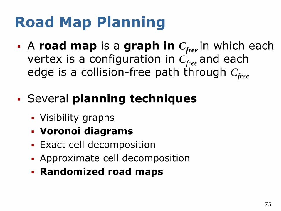
Road Map Planning
A road map is a graph in Cfree in which each vertex is a configuration in Cfree and each edge is a collision-free path through Cfree
Several planning techniques
Visibility graphs
Voronoi diagrams
Exact cell decomposition
Approximate cell decomposition
Randomized road maps
75

Defined to be the set of points q whose
cardinality of the set of boundary points of Cobs with the same distance to q is greater
than 1
Let us decipher this definition...
Informally: the place with the same maximal clearance from all nearest obstacles
Generalized Voronoi Diagram
76
qI qG
qI' qG'

Formally:
Let be the boundary of Cfree, and d(p,q) the Euclidian distance between p and q. Then, for all q in Cfree, let
be the clearance of q, and
the set of "base" points on with the same clearance to q. The Voronoi diagram is then the set of q's with more than one base point p
Generalized Voronoi Diagram
77

Geometrically:
For a polygonal Cobs, the Voronoi diagram consists of (n) lines and parabolic segments
Naive algorithm: O(n4), best: O(n log n)
Generalized Voronoi Diagram
78
p
clearance(q)
one closest point
q
q
q
p p
two closest points
p p

Voronoi Diagram
Voronoi diagrams have been well studied for (reactive) mobile robot path planning
Fast methods exist to compute and update the diagram in real-time for low-dim. C's
Pros: maximize clear- ance is a good idea for an uncertain robot
Cons: unnatural at- traction to open space, suboptimal paths
Needs extensions 79
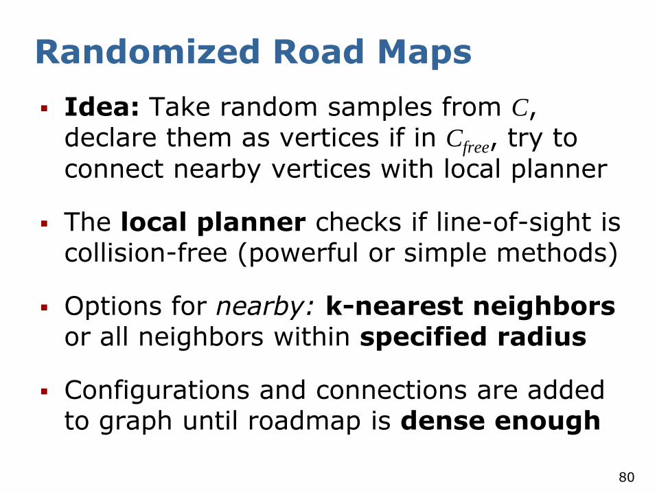
Randomized Road Maps
Idea: Take random samples from C, declare them as vertices if in Cfree, try to
connect nearby vertices with local planner
The local planner checks if line-of-sight is collision-free (powerful or simple methods)
Options for nearby: k-nearest neighbors or all neighbors within specified radius
Configurations and connections are added to graph until roadmap is dense enough
80

Randomized Road Maps
Example
81
specified radius
Example local planner
What does “nearby” mean on a manifold? Defining a good metric on C is crucial

Randomized Road Maps
Pros:
Probabilistically complete
Do not construct C-space
Apply easily to high dimensional C-spaces
Randomized road maps have solved previously unsolved problems
Cons:
Do not work well for some problems, narrow passages
Not optimal, not complete
82
Cobs
Cobs
Cobs
Cobs Cobs
Cobs Cobs
qI
qG
qI
qG

Randomized Road Maps
How to uniformly sample C ? This is not at all
trivial given its topology
For example over spaces of rotations: Sampling Euler angles gives more samples near poles, not uniform over SO(3). Use quaternions!
However, Randomized Road Maps are powerful, popular and many extensions exist: advanced sampling strategies (e.g. near obstacles), PRMs for deformable objects, closed-chain systems, etc.
83

From Road Maps to Paths
All methods discussed so far construct a road map (without considering the query pair qI and qG)
Once the investment is made, the same road map can be reused for all queries (provided world and robot do not change)
1. Find the cell/vertex that contain/is close to qI and qG (not needed for visibility graphs)
2. Connect qI and qG to the road map
3. Search the road map for a path from qI to qG
84

Consider an agent acting in this environment
Its mission is to reach the goal marked by +1 avoiding the cell labelled -1
Markov Decision Process
85
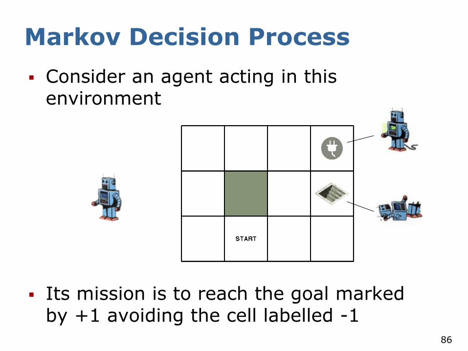
Consider an agent acting in this environment
Its mission is to reach the goal marked by +1 avoiding the cell labelled -1
Markov Decision Process
86

Markov Decision Process
Easy! Use a search algorithm such as A*
Best solution (shortest path) is the action sequence [Right, Up, Up, Right]
87

What is the problem?
Consider a non-perfect system in which actions are performed with a probability less than 1
What are the best actions for an agent under this constraint?
Example: a mobile robot does not exactly perform a desired motion
Example: human navigation
Uncertainty about performing actions!
88
MDP Example
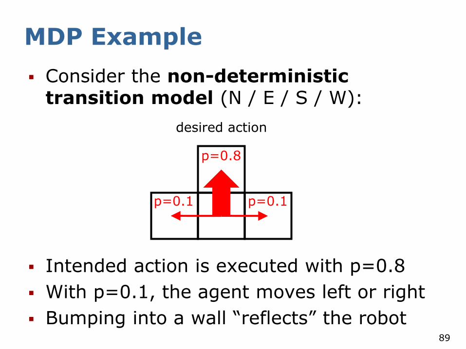
Consider the non-deterministic transition model (N / E / S / W):
Intended action is executed with p=0.8
With p=0.1, the agent moves left or right
Bumping into a wall “reflects” the robot
desired action
p=0.8
p=0.1 p=0.1
89
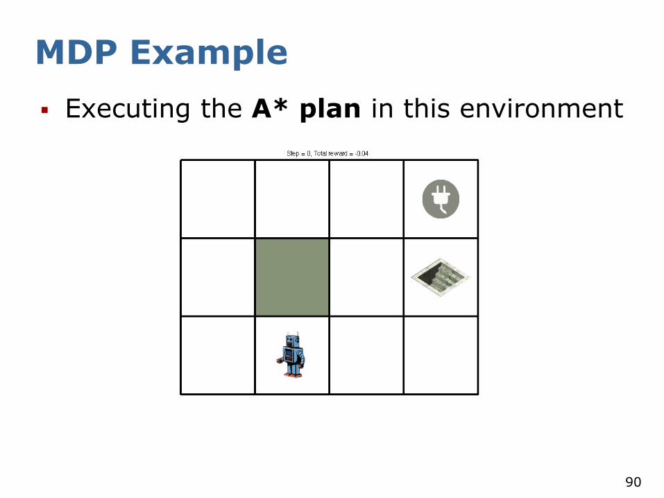
MDP Example
Executing the A* plan in this environment
90

MDP Example
Executing the A* plan in this environment
But: transitions are non-deterministic!
91

MDP Example
Executing the A* plan in this environment
This will happen sooner or later...
92

MDP Example
Use a longer path with lower probability to end up in cell labelled -1
This path has the highest overall utility
Probability 0.86 = 0.2621 93

Transition Model
The probability to reach the next state s' from state s by choosing action a
is called transition model
94
Markov Property:
The transition probabilities from s to s' depend only on the current state s and not on the history of earlier states

Reward
In each state s, the agent receives a reward R(s)
The reward may be positive or negative but must be bounded
This can be generalized to be a function R(s,a,s'). Here: consider only R(s), does not
change the problem
95

Reward
In our example, the reward is -0.04 in all states (e.g. the cost of motion) except the terminal states (that have rewards +1/-1)
A negative reward gives agent an in- centive to reach the goal quickly
Or: “living in this environment is not enjoyable”
96

MDP Definition
Given a sequential decision problem in a fully observable, stochastic environment with a known Markovian transition model
Then a Markov Decision Process is defined by the components
• Set of states:
• Set of actions:
• Initial state:
• Transition model:
• Reward funciton:
97

Policy
An MDP solution is called policy p
A policy is a mapping from states to actions
In each state, a policy tells the agent what to do next
Let p (s) be the action that p specifies for s
Among the many policies that solve an MDP, the optimal policy p* is what we seek. We'll see later what optimal means
98

Policy
The optimal policy for our example
99
Conservative choice Take long way around
as the cost per step of -0.04 is small compared with the penality to fall
down the stairs and receive a -1 reward

Policy
When the balance of risk and reward changes, other policies are optimal
100
R < -1.63
-0.02 < R < 0
-0.43 < R < -0.09
R > 0
Leave as soon as possible Take shortcut, minor risks
No risks are taken Never leave (inf. #policies)

Utility of a State
The utility of a state U(s) quantifies the
benefit of a state for the overall task
We first define Up(s) to be the expected
utility of all state sequences that start in s given p
U(s) evaluates (and encapsulates) all possible futures from s onwards
101

Utility of a State
With this definition, we can express Up(s) as a function of its next state s'
102

Optimal Policy
The utility of a state allows us to apply the Maximum Expected Utility principle to define the optimal policy p*
The optimal policy p* in s chooses the action a that maximizes the expected utility of s (and of s')
Expectation taken over all policies
103

Optimal Policy
Substituting Up(s)
Recall that E[X] is the weighted average of all possible values that X can take on
104

Utility of a State
The true utility of a state U(s) is then
obtained by application of the optimal policy, i.e. . We find
105

Utility of a State
This result is noteworthy:
We have found a direct relationship between the utility of a state and the utility of its neighbors
The utility of a state is the immediate reward for that state plus the expected utility of the next state, provided the agent chooses the optimal action
106

Bellman Equation
For each state there is a Bellman equation to compute its utility
There are n states and n unknowns
Solve the system using Linear Algebra?
No! The max-operator that chooses the optimal action makes the system nonlinear
We must go for an iterative approach 107

Discounting
We have made a simplification on the way:
The utility of a state sequence is often defined as the sum of discounted rewards
with being the discount factor
Discounting says that future rewards are less significant than current rewards. This is a natural model for many domains
The other expressions change accordingly
108

Separability
We have made an assumption on the way:
Not all utility functions (for state sequences) can be used
The utility function must have the property of separability (a.k.a. station-arity), e.g. additive utility functions:
Loosely speaking: the preference between two state sequences is unchanged over different start states
109

Utility of a State
The state utilities for our example
Note that utilities are higher closer to the goal as fewer steps are needed to reach it
110

Idea:
The utility is computed iteratively:
Optimal utility:
Abort, if change in utility is below a threshold
Iterative Computation
111

The utility function is the basis for “Dynamic Programming”
Fast solution to compute n-step decision
problems
Naive solution: O( |A|n )
Dynamic Programming: O( n |A| |S| )
But: what is the correct value of n?
If the graph has loops:
Dynamic Programming
112
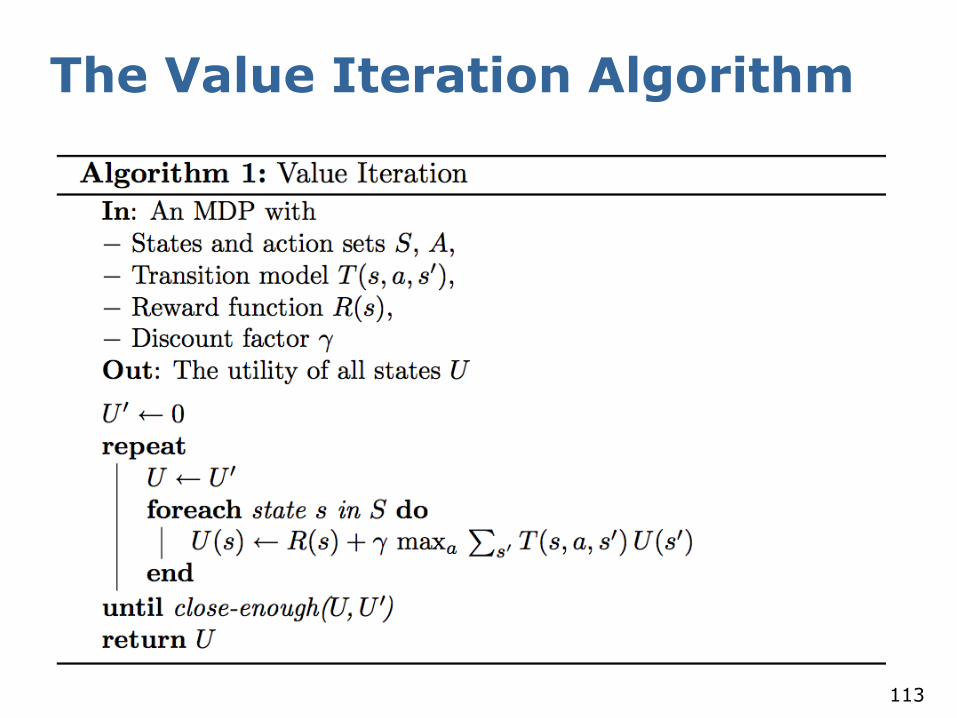
The Value Iteration Algorithm
113

Calculate utility of the center cell
Value Iteration Example
u=10
u=-8 u=5
u=1
r=1
Transition Model State space
(u=utility, r=reward)
desired action = Up
p=0.8
p=0.1 p=0.1
114

Value Iteration Example
u=10
u=-8 u=5
u=1
r=1
115

Value Iteration Example
In our example
States far from the goal first accumulate negative rewards until a path is found to the goal
116
(1,1) nr. of iterations →

Convergence
The condition in the algorithm can be formulated by
Different ways to detect convergence:
RMS error: root mean square error
Max error:
Policy loss
117
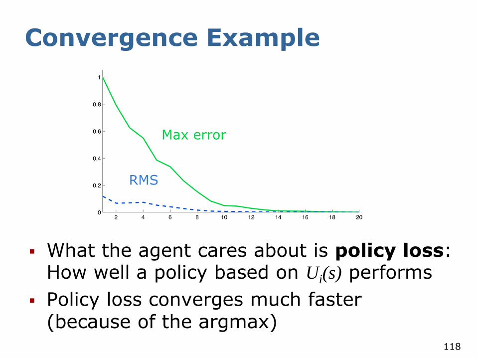
Convergence Example
What the agent cares about is policy loss: How well a policy based on Ui(s) performs
Policy loss converges much faster (because of the argmax)
RMS
Max error
118

Value Iteration
Value Iteration finds the optimal solution to the Markov Decision Problem!
Converges to the unique solution of the Bellman equation system
Initial values for U' are arbitrary
Proof involves the concept of contraction. with B being
the Bellman operator (see textbook)
VI propagates information through the state space by means of local updates
119
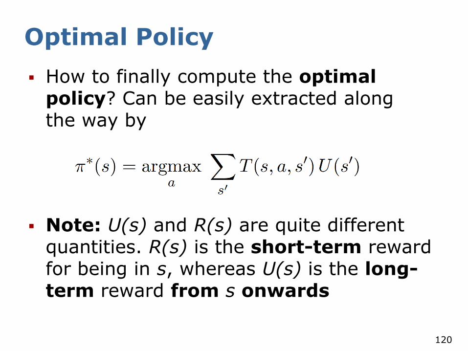
Optimal Policy
How to finally compute the optimal policy? Can be easily extracted along the way by
Note: U(s) and R(s) are quite different quantities. R(s) is the short-term reward for being in s, whereas U(s) is the long-term reward from s onwards
120

121
Summary
Robust navigation requires combined path planning & collision avoidance.
Approaches need to consider robot's kinematic constraints and plans in the velocity space.
Combination of search and reactive techniques show better results than the pure DWA in a variety of situations.
Using the 5D-approach the quality of the trajectory scales with the performance of the underlying hardware.
The resulting paths are often close to the optimal ones.

122
Summary
Planning is a complex problem.
Focus on subset of the configuration space:
road maps,
grids.
Sampling algorithms are faster and have a trade-off between optimality and speed.
Uncertainty in motion leads to the need of Markov Decision Problems.
123
What’s Missing?
More complex vehicles (e.g., cars).
Moving obstacles, motion prediction.
High dimensional spaces.
Heuristics for improved performances.
Learning.