Introduction to Microeconomics Production, cost and profit in the short-run

Introduction to Microeconomics

Production, cost and profit in the short-run

You should understand how • Opportunity cost shapes supply • Law of diminishing marginal returns is related to marginal and average

product.

• Total, average, and marginal product are related • To identify the short-run profit point • The firm decides on how much to produce and how many employees to

hire.• To show the maximum profit point graphically• How costs and the availability of inputs affect short-run supply curve

and elasticity of supply.

Learning Objectives

Key ideas

Copyright © 2012 McGraw-Hill Ryerson Limited

Ch5-2

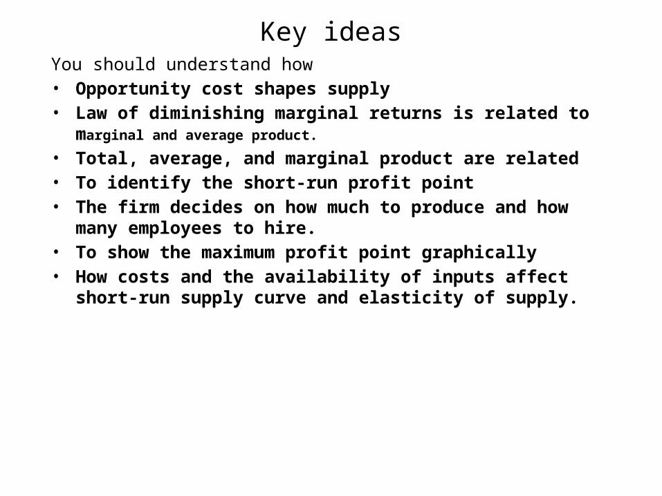
This chapter rests on two assumptions1. The firm operates under perfect competition

• Buyers and sellers are fully informed• There are many buyers and sellers – no market participant can

influence supply• This means that firms are “price-takers”

2. Short-run decisions (Short-run is an imprecise idea, but means that businesses cannot adjust equipment, leases and is stuck with other contracts

Opportunity cost• For this class, today … the value of the next best way to spend your

time• For a business … the value of what could be produced using the

resources available

Short-run for a business• Must work within the equipment and contracts available now• The time period over which a business can change equipment and

contracts, starts to define the line between short and longer-run.

• Firms are believed to maximize profits as a primary goal.

• Price taker– A firm that has no influence over the price at

which it sells its product.• Profit

– Total revenue (price x the quantity) minus all costs of production.

Profit Maximization


Ch5-4LO2: Law of Diminishing Marginal Product and

Average and Marginal Product

• Factor of Production– An input used in the production of a good or service.– Four categories: land labour, capital, or

entrepreneurship.

• Intermediate input – an input that is used up in the production process– natural resources

• Other? • Innovation? • Energy?

Key terms

Cost and Benefit principle

Costs of production will increase as output increases, but since the price remains the same – at some point the additional (marginal) cost of producing one more unit will start to exceed the additional (marginal) revenue gained from the sale of that additional unit.

Profit maximization means that

Marginal cost = marginal revenue

Law of Diminishing Marginal Returns (for labour)

Given that all other inputs and technology are fixed, the marginal product of labour increases, and then decreases as successively more units of labour are employed.

A Short Run Production Function of Acme Glass Limited

Total outputof bottles

Average product

Marginal product

Maximum MP

Maximum AP


Ch5-7LO3: Graphing the Relationships

among Total, Average and Marginal Values

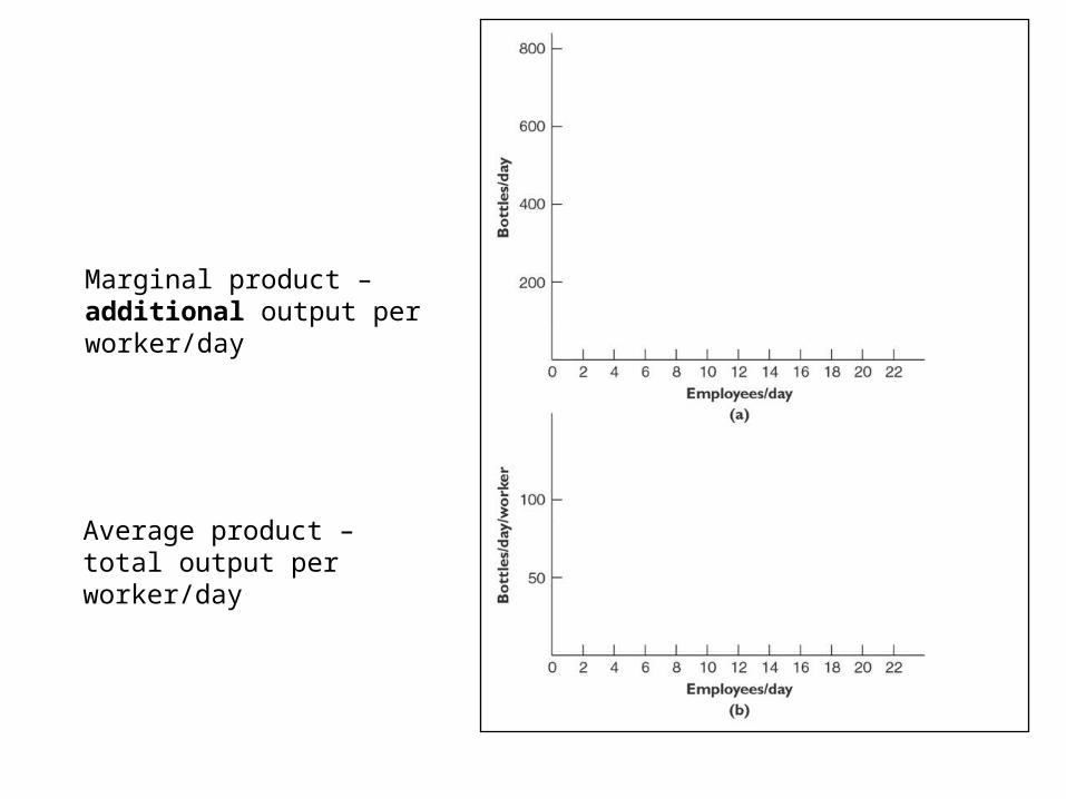
Marginal product – additional output per worker/day

Average product – total output per worker/day

• When total product reaches maximum, marginal product is equal to 0.

• Maximum marginal product occurs to the left of maximum average product.

• Marginal product intersects average product at its maximum.

• If marginal product exceeds average product, then average product is rising.

• If marginal product is less than average product, then average product is falling.

Total Output, Marginal Product, and Average Product for a Glass-Bottle

Maker

Total product of labour

Average product

Marginal product

Maximum TP

Maximum MP

MP = 0

Maximum AP


Ch5-8LO3: Graphing the Relationships

among Total, Average and Marginal Values

Employment, Output, Revenue, Costs, and Profit of Acme Glass Limited

Employee wage rate = $10/day; Price of bottles = $35/hundred = $0.35/bottle

Profit maximization choice


LO4: Maximizing Short Run Profit Ch5-15

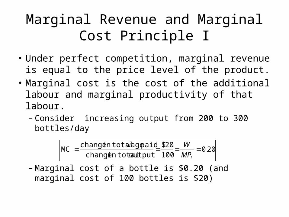
• Under perfect competition, marginal revenue is equal to the price level of the product.

• Marginal cost is the cost of the additional labour and marginal productivity of that labour.– Consider increasing output from 200 to 300

bottles/day

– Marginal cost of a bottle is $0.20 (and marginal cost of 100 bottles is $20)

LO5: Firm’s Cost and Decision on Quantity Supplied and Hiring

Marginal Revenue and Marginal Cost Principle I

20.0100

20$

output totalin change

paid wage totalin changeMC

LMP

W


Ch5-10

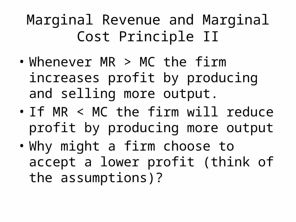
• Whenever MR > MC the firm increases profit by producing and selling more output.

• If MR < MC the firm will reduce profit by producing more output

• Why might a firm choose to accept a lower profit (think of the assumptions)?


Marginal Revenue and Marginal Cost Principle II


Ch5-11


TABLE 5.3: Employment, Output, Revenue, Costs, and Profit at Acme Glass Limited

Example 5.2: Employee wage rate = $10/day; Price of bottles = $0.45/bottle



Ch5-12


TABLE 5.4: Employment, Output, Revenue, Costs, and Profit at Acme Glass Limited

Example 5.3: Employee wage rate = $14/day; Price of bottles = $0.35/bottle



Ch5-13

– The firm’s cost goes up by $20 when it expands production from 200 to 300 bottles/day. The marginal cost of the increased output is thus $20. By convention we plot that value at a point midway between 200 and 300 bottles/day.

Acme’s Marginal Cost of Production

The firm’s cost goes up by $20 when it expands production from 200 to 300 bottles/day.


Ch5-14LO5: Firm’s Cost and Decision on

Quantity Supplied and Hiring

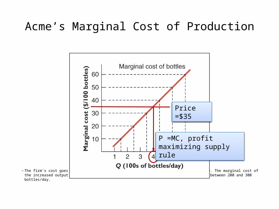
– The firm’s cost goes up by $20 when it expands production from 200 to 300 bottles/day. The marginal cost of the increased output is thus $20. By convention we plot that value at a point midway between 200 and 300 bottles/day.

Acme’s Marginal Cost of Production

Price =$35

P =MC, profit maximizing supply rule




A Shift of the MarginalCost Curve

Labour cost increases from$10 to $14/day and causesMC to shift to MC .




TABLE 5.5: The Law of Diminishing Marginal Returns and Short-Run Costs for Acme Glass (at a daily wage of $10)

LO6: Short Run Cost and Product Curve

∆(2)/∆(1)La

w o

f dim

inis

hing

mar

gina

l ret

urns


Ch5-17

• MC = ∆TC/∆Q • TC = Variable costs + Fixed Costs• AVC = TVC/Q• AFC = TFC/Q• ATC = AFC + AVC

– Short-run cost-minimizing quantity of output :• the quantity of output at which a factory reaches

minimum average total cost.

Short-run Costs

LO6: Short Run Cost and Product CurveCopyright © 2012 McGraw-Hill Ryerson Limited

Ch5-18

• When marginal product reaches its maximum, marginal cost is at its minimum. And when average product reaches its maximum, average variable cost is at its minimum.

• Marginal product intersects average product at maximum average product, marginal cost intersects average variable cost at minimum average variable cost.

• The two sets of curves are mirror images of each other.

FIGURE 5.5: The Relationship between Product Curves and Cost

Curves

Marginal cost

Marginal product

Average variable cost

Minimum average variable cost

Minimum marginal cost

Average product

Maximum average product

Maximum marginal product


Ch5-19LO6: Short Run Cost and Product Curve

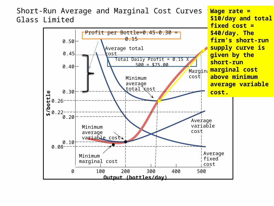
Short-Run Average and Marginal Cost Curves for Acme Glass Limited

Minimum marginal cost

Minimum averagevariable cost

Minimum averagetotal cost

Average total cost

Marginal cost

Average variable cost

Average fixed cost

0 100 200 300 400 500

0.50

0.40

0.30

0.20

0.08

0.22

0.26

0.10

Output (bottles/day)

$/b

ott

le


Ch5-20LO7: Price Takers Maximum Profit

Profit per Bottle=0.45-0.30 = 0.15

Total Daily Profit = 0.15 X 500 = $75.00

0.45

Wage rate = $10/day and total fixed cost = $40/day. The firm’s short-run supply curve is given by the short-run marginal cost above minimum average variable cost.

– If price drops below minimum average variable cost, the firm will minimize its losses by shutting down.

– What this means is that if the costs of variable inputs (wages, supplies, etc.) per unit of output cannot be covered by price per unit, send everyone home…it is cheaper.

The Shut-Down Rule


Ch5-21LO7: Price Takers Maximum Profit

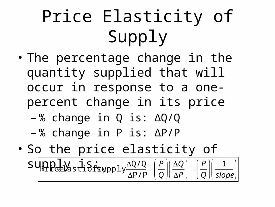
• The percentage change in the quantity supplied that will occur in response to a one-percent change in its price– % change in Q is: ΔQ/Q– % change in P is: ΔP/P

• So the price elasticity of supply is:

Price Elasticity of Supply

slopeQ

P

P

Q

Q

P 1

P/P

Q/Qsupply of elasticity Price


Ch5-22LO8: The Price Elasticity of Supply

• Fertile agricultural land is a historically scarce resource. Is this true?

• Since it makes sense to use the most fertile land first, as the amount of land under cultivation expands, eventually less fertile land will have to be used.

Then why are cities often on the best land?• Cost of production will rise as farmers start to use less fertile

land. What options exist?

• When an essential input into production is inherently limited in availability, the supply curve will be upward sloping, even in the long run.

Unique and Essential Inputs: The Ultimate Supply Bottleneck

LO8: The Price Elasticity of Supply Copyright © 2012 McGraw-Hill Ryerson Limited

Ch5-23

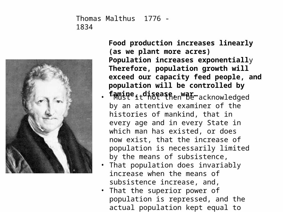
• “Must it not then be acknowledged by an attentive examiner of the histories of mankind, that in every age and in every State in which man has existed, or does now exist, that the increase of population is necessarily limited by the means of subsistence,

• That population does invariably increase when the means of subsistence increase, and,

• That the superior power of population is repressed, and the actual population kept equal to the means of subsistence, by misery and vice.”

Thomas Malthus 1776 - 1834

Food production increases linearly (as we plant more acres)Population increases exponentiallyTherefore, population growth will exceed our capacity feed people, and population will be controlled by famine, disease, war…

Malthusian trap

• Population has risen many times since Malthus’ day• Yet we have been able to feed people• Why

Other “Malthusian” Statements

• Over-fishing – certain species are either close to extinct or is short supply (essentially fixed)

– As demand expands ( think tuna and sushi) the price of tuna and sushi rises

– Other fish are substituted– Some consumers switch (price and income substitution)

• Peak oil - the world is running out of oil– What will we do?

The Green Revolution

• Price/cost increases pinch profit margins• Innovation is spurred• The “green revolution” refers to advances in

farming technology (Techniques, fertilization, pesticide, herbicide, new species).

• Genetically modified organisms (GMO) technology

GMO• Genetic engineering, also called genetic

modification, is the direct manipulation of an organism's genome using biotechnology. New

DNA may be inserted in the host genome by first isolating and copying the genetic material of interest using molecular cloning methods to generate a DNA sequence, or by synthesizing

the DNA, and then inserting this construct into the host organism.

http://en.wikipedia.org/wiki/Genetic_engineering (accessed Oct 14, 2012)

http://en.wikipedia.org/wiki/Genome

http://en.wikipedia.org/wiki/Biotechnology

http://en.wikipedia.org/wiki/DNA

http://en.wikipedia.org/wiki/Molecular_cloning

http://en.wikipedia.org/wiki/Genetic_engineering

http://en.wikipedia.org/wiki/Genetic_engineering

Traditional vs. GMO methods• Classical plant breeding uses deliberate interbreeding (crossing) of closely or

distantly related individuals to produce new crop varieties or lines with desirable properties. Plants are crossbred to introduce traits/genes from one variety or line into a new genetic background.– Advantage is that it is time tested (used for many centuries) to change crops

and animals to have desirable traits• Higher milk production• Resistance to disease

– Disadvantage is that it is slow, and requires many cycles and trial and error to breed in the desirable trait

• Genetic engineering is more precise and faster.– Fears exist that these are not safe– Few understand the process– Tends to vests a lost of control in a few large multinationals (Monsanto)

http://en.wikipedia.org/wiki/Trait_(biological)

http://en.wikipedia.org/wiki/Gene

Documents

Introduction to Microeconomics Production, cost and profit in the short-run