Chapter 4

Introduction to Maxwell’sTheory

Z

X

YQQ11

QQ22

FF2211

EE((rr))

TTHHEE EELLEECCTTRRIICC FFIIEELLDD

Figure 4.1: The Electric Field and Electric Forces Maxwell said thatelectric and magnetic forces were due to the presence of the electric andmagnetic field. In this figure, the electric force on Q2 is due to the presenceof the field at its location, �F21 = Q2

�E(�r). There is a similar relationship forthe magnetic force.

Maxwell was interested in developing a mechanical basis for the phe-nomena associated with electricity and magnetism, [Maxwell 1861]. In thosedays and especially to Maxwell, a mechanical basis was one that could ulti-mately be traced to an underly atomic constituent and simple force relation-ships. In addition to providing a mechanical “explaination”, he could alsoshow that electric and magnetic phenomena were inter-related phenomena,

63

64 CHAPTER 4. INTRODUCTION TO MAXWELL’S THEORY

i. e. unifying the two force systems.In his time, many of the basic ideas of the electric and magnetic force

systems were known. The law for the electric interaction between chargedparticles had been articulated in the period 1785 and 1791 by Coulomb. Theforce law between magnets and the force between moving charges and mag-nets was known and even Faraday’s Law about the relationship of changingmagnetic environments and electric currents was known. In fact, Faradayhad already began to describe magnetic and electric phenomena in a fieldlike language. What Maxwell sought was an underlying mechanical basisfor all the phenomena associated with electricity and magnetism. Reducingelectricity and magnetism to a mechanical basis meant that he was lookingfor something to push or pull but it had to do so locally. He could notbelieve that fundamental phenomena could take place as an action at dis-tance phenomena like gravity was thought to be at the time. In order tohave a thing which could push or pull locally, he hypothesized the existenceof a rather rich structure for the vacuum of space, whirling vortices in anether that produced the electric and magnetic force. These were to be hisatoms. This was an obvious extension of the prevailing ideas used in fluidflow. Fluids seemed continuous systems that had smooth spatial propertiesand produced macroscopic forces but were composed of the underly atoms.Regardless, the flow mechanics was well described by a field dynamic. Thusnot only did he seek a mechanical source for electric and magnetic phenom-ena, he developed a field theory basis for it. His picture of electric andmagnetic forces was that they were mediated by fields, the electric, �E, andthe magnetic, �B, fields. It was his basic idea that the correct description ofelectromagnetic phenomena required a locally causal dynamic The idea wasthat not only did the charges generated the fields but the fields themselvesresponded to the local environment of the fields themselves. In addition, theforces experienced by the charges were because of the values of the fields atthe place occupied by the charges, �F = q �E + q�v × �B, where q is the chargein question and �v is its velocity.

In order to create the mechanical basis for the fields, Maxwell was forcedto endowed the ether with the correct mechanical properties of inertia andsize to replicate the success of the earlier laws but now in context of alocal mechanical model. The underlying idea was simple. Let’s look at thesimplest of the cases, Coulomb’s Law. The situation is shown in Figures 4.2and 4.3. A force on a charged particle took place as a two step process. Acharge Q1 is placed in empty unexcited space. This charge excites the ethernext to it by creating vortices at its location. These vortices in turn exciteneighboring vortices until space is full of whirling vortices. Each vortex is in

65

Q1

x

y

z

r

Figure 4.2: Maxwell’s Vortices Maxwell pictured the electric force asemerging in two steps. First any charged particle would excite vortices inthe ether at its location. These vortices would excite other vortices nearbyand so forth until all of space would fill with whirling vortices. In a sense,the whirliness of the vortices at any place was a measure of the strength ofthe electric field at that point.

dynamic equilibrium with its neighbors. There is a ‘thing’, the whirliness,which is a measure of the electric field at that point.

When a new charge, Q2, is located at some distance, �r, from the firstcharge, it detects the level of excitement of the local vortices and thus feelsa corresponding force. The force is proportional to the charge Q2 at thatplace and the amount of whirliness or electric field at that point.

The mechanical properties of the ether and its vortices determine howthe whirliness develops. This is set by the vortices inertia and size. Theseparameters for the mechanical properties of the vortices are then adjustedto accommodate Coulomb’s Law.

In other words, Maxwell introduced local fields – a continuous quantitydefined at all points in space and for all times – with a rule of dynamics toproduce the electromagnetic forces. If an object experiences a force, theremust be something at that place, the whirliness. In addition, the whirlinessitself must be determined locally in both space and time. Let’s go throughthe example of Coulomb’s Law in a little more detail to see how this ideaworks.

The first problem is to reproduce the well known Coulomb’s law of force

66 CHAPTER 4. INTRODUCTION TO MAXWELL’S THEORY

Q1

x

y

z

rQ2

Figure 4.3: Vortices and the Electric Force When a charged particle,Q2, is positioned, the particle detects the local amount of whirliness in thevortices of the ether. This generates the electric force in proportion to thecharge and amount of whirliness at its location. The local whirliness is �Eat �r.

for static situations. Coulomb’s Law is an action at a distance descriptionof interaction,

�F21 =1

4π�0

Q1Q2

r212

�r21

r12(4.1)

where �r12 is the separation between the charges. In order to simplify thediscussion, let’s place charge Q1 at the origin. Since the force on the chargeQ2 is supposed to be Q2

�E(�r), where �r is now the position at which Q2 islocated. For this case, we can identify the electric field as

�E(�r) =1

4π�0

Q1

r2

�r

r(4.2)

around a spherically symmetric charge placed at the origin. You will repro-duce the static Coulomb’s Law results with the electric field if you can makea local rule about how �E(�r) develops that reproduces this result. It shouldbe clear that the hard part will be to reproduce the inverse square fall offwith distance in the strength of the field.

In some sense, it is really not correct to say that Q1 is the source of thisfield. The field is not attached to the charge. At any point, there is a fieldonly if there is a field or a charge in the neighborhood. The field at some

67

point, like all things, is to be determined locally. Maxwell used his whirlingvortices of the ether to discover a rule for whirliness and how whirlinesseffected whirliness that recovers the characteristic the inverse square fall offwith distance of Coulomb’s Law. Like the stretched sting, Section 2.2, inwhich the transverse position of a place on the string is determined by thetransverse position of the neighbors to that place, similarly here, the idea isto find the rule on how the field arranges itself and forget about the whirlies.The following analysis reviews the process and becomes somewhat technicalbut the struggle to follow it is worth the effort.

Since the electric field is meant to produce a force, it must be a vectorfield, a directed quantity defined at every point in space and with a localrule for its construction. Basically you ask how much does the field changeat a place because of what is there. For now, we are looking at a static case– no time change. But we can still ask about how the field varies as wechange positions in space.

For a vector field such as the electric field since it is a vector field,you have a directed strength at each point in space and around each pointyou have directed strengths. At any point you can ask how much more“outpointy” these directed strengths become as you go from place to place.The analogy for our stretched string is that, at any place on the string, youcan ask how “bendy” is the string. On a string, “bendiness” happens whenthat place differs from its neighbors. The string bends up when the place islower than its neighbors and it bends down when it is higher. When thereis no bend, that place on the string is at the average of its neighbors. In thestatic string it takes a force to maintain a bend in the string. Our case forthe vector field case using “outpointiness” works in the same fashion. Youcan have “outpointiness” only if there are charges that are placed there,i. e. charge causes an outward directed field. Of course, we have to developa definition, a measure, of “outpointy” and test it.

The measure of “outpointiness” is called the divergence and it is whatyou would have thought to define it as if you spent some time playing withthe ideas of a vector field. At any point, find out how much the neighboringfields point away from where you are. That should indicate the “outpointi-ness”.

Since fluid flow is also a vector field it is worthwhile to think in terms ofit. The vector field in this case is the velocity of the fluid. If at a point allthe flow is uniform about you, you would not think of the field as becoming“out pointy”. On the other hand, if you were at a place like the drain,you would consider the surrounding flow to be “inpointy”, the opposite of“outpointy”. To be more quantitative, think of surrounding the place that

68 CHAPTER 4. INTRODUCTION TO MAXWELL’S THEORY

Figure 4.4: Construction of the Divergence To find the divergence or“outpointiness” of a vector field at a point, surround the point with a surface,step (a). Cover the surface with small elements of area so that to all intentsand purposes they can be considered flat. Each element of surface will nowhave a normal vector. Find the magnitude of the vector field at the surfaceto is along the surface. Add these magnitudes for each element of surfaceand the total is the divergence or “outpointiness” of the vector field at thepoint surrounded by the surface. Then shrink the volume surrounded to apoint. For a fluid, applied to the velocity field, this tells the amount of fluidthat goes into a point. This series of steps is encoded in the first part ofEquation 4.4 for the case of the electric field.

you are interested in and measuring how much stuff flows in or out. Byenclosing the point of interest with a surface, we can measure the incomingfluid by assessing how much stuff comes into any element of area on thesurrounding surface and then adding the contribution to each part. In otherwords, surround the point with a surface. Cover it with elements of area,postage stamps labeled ∆2s. Each element of area has a normal vector, s,that points either outward or inward, see Figure 4.4. Choosing the outwardnormal, we are defining “outpointiness”, the amount of the vector field thatis along the outward normal; it is the “flow” through that element of area.Now do this for the each element of the entire surface and add up all thecontribution from all the pieces,

�S⊃V

. To reduce this analysis to a point,shrink the volume enclosed by the surrounding surface to zero, limV→0.This same analysis holds for all vector fields. This construction at eachpoint assesses the “outpointiness” of the neighborhood of the point and iscalled the divergence. Thus,

Div(�E)(�r) ≡ limV→0

�S⊃V

�E(�r �) ·�∆2ss

�

V≡ lim

V→0

�S⊃V

�E(�r �) · s d2s

V(4.3)

69

= limV→0

1�0

Qinside V

V=

1�0

ρ(�r) (4.4)

where the first part is a mathematical statement of what is stated abovefor the definition of the divergence but for the case of the electric field andthe subsequent parts are the relationship with charge that is necessary torecover Coulomb’s Law, i. e. electric charge is the source of “outpointiness”of the electric field. Note that the divergence of a vector field, Div(�E)(�r), isa scalar field. In cartesian coordinates, the divergence is simply written

Div(�E)(�r) =∂Ex(�r)

∂x+

∂Ey(�r)∂y

+∂Ez(�r)

∂z. (4.5)

QQeenncc

EE((rr))EE((rr))

EE((rr))

EE((rr))

EE((rr))

EE((rr))

EE((rr))

EE((rr))

EE((rr))

EE((rr))

EE((rr))

EE((rr))

EE((rr))

EE((rr))EE((rr))

EE((rr))

EE((rr)) iiss aa DDiivveerrggiinngg FFiieelldd

Figure 4.5: ”Outpointiness of the Electric Field” A characteristic prop-erty of the electric field is that charge is the source of “outpointiness”. Thisis the idea that the electric field points away from nearby positive chargesand toward nearby negative charges. This last example being negative out-pointiness.

Notice that this law, Equation 4.4, says that for a static electric fieldthere is divergence of the field only where there is charge. Yet the picturethat we all have of the static electric field around an isolated point charge is adiverging field, the electric field points outward from the origin everywhere,see Figure 4.5. How do we reconcile this?

Consider a point away from the isolated point charge. If a surface such asthat shown in Figure 4.4 is constructed area at nearer the charge is smallerwhereas the area more distant is larger. In fact, the areas are in the ratioof the distances squared. Thus the field strength and the areas combineso that the net “outpointiness”, actually inpointiness, of the nearer surface

70 CHAPTER 4. INTRODUCTION TO MAXWELL’S THEORY

!far"far

"near!near

Point Chargeat origin

Figure 4.6: Divergence Outside of Charge A characteristic propertyof the electric field is that charge is the source of “outpointiness”. Thisis the idea that the electric field points away from nearby positive chargesand toward nearby negative charges. This last example being negative out-pointyness.

balances the outpointiness of the far surface and the net is zero. Thus it isbecause the divergence is zero at places other than the charge that the fieldstrength falls off with distance as 1

r2 .Another property that a vector field can manifest is a rotation or curl.

The curl of a vector field is itself a vector field. Again you develop a definitionand test it. The first step is to pick a small plane area surrounding the pointof interest, ss, where again s is the unit normal to the area. Remember thatarea is a directed quantity and thus a vector. The area is bounded by aclosed path �r �(z), 0 ≤ z ≤ 1, �r �(z) ⊂ s. The component of the curl alongthe s direction at the point is the amount of the field circulating with thetangents to the path �r �(z). In other words, the idea is to follow a closedpath around the point and see how much of the vector field follows the path.Varying all directions for s the value of the curl at the point p is maximumobtained and the curl is directed in that direction. Another way to findthe value of the vector field that is curl of a vector field is to establish threeindependent orthogonal directions for the areas, a coordinate frame, and theobtained values are then the three components of the vector field. In thestatic case, the electric field does not have curl.

→Curl(�E(�r)) · s ≡ lim

s→0

��r �⊃S

�E(�r �) ·∆�r

�

∆z∆z

s(4.6)

71

≡ lims→0

��r �⊃S

�E(�r �) ·d�r

�

dzdz

s= 0. (4.7)

The curl in cartesian coordinates takes the simple form

→Curl (�E)(�r) =

�∂Ey

∂z−

∂Ez

∂y

�x +

�∂Ez

∂x−

∂Ex

∂z

�y +

�∂Ex

∂y−

∂Ey

∂x

�z

(4.8)On the other hand, the magnetic field does curl. The magnetic field is

the force experienced by a moving charged particle.

�Fmag = Q�v × �B(�r). (4.9)

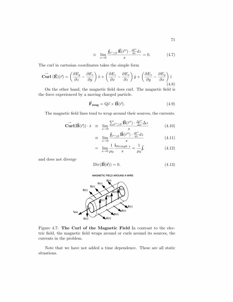
The magnetic field lines tend to wrap around their sources, the currents.

→Curl(�B(�r)) · s ≡ lim

s→0

��r �⊃S

�B(�r �) ·∆�r

�

∆z∆z

s(4.10)

≡ lims→0

��r �⊃S

�B(�r �) ·d�r

�

dzdz

s(4.11)

= lims→0

1µ0

ithrough s

s=

1µ0

�j, (4.12)

and does not divergeDiv(�B(�r)) = 0. (4.13)

iieenncc

BB((rr))

MMAAGGNNEETTIICC FFIIEELLDD AARROOUUNNDD AA WWIIRREE

BB((rr))BB((rr))

BB((rr))

BB((rr)) BB((rr))BB((rr))

BB((rr))BB((rr))

BB((rr))BB((rr))

BB((rr))BB((rr))

Figure 4.7: The Curl of the Magnetic Field In contrast to the elec-tric field, the magnetic field wraps around or curls around its sources, thecurrents in the problem.

Note that we have not added a time dependence. These are all staticsituations.

72 CHAPTER 4. INTRODUCTION TO MAXWELL’S THEORY

Maxwell insisted that the field was not established everywhere at once.It was made up of whirling vortices that pushed on each other. The rateat which the vortices could push was set by the parameters of the statictheory. By endowing these whirling vortices with the correct properties toreproduce the laws of static electricity and magnetism, he found how to adda local set of rules for the time evolution of the fields. These are the full setof Maxwell’s equations including time dependence:

Div(�E(�r, t)) =1�0

ρ(�r, t) (4.14)

→Curl(�E(�r, t)) =

∂�B∂t

(�r, t) (4.15)

Div(�B(�r, t)) = 0 (4.16)→

Curl(�B(�r, t)) = µ0�j(�r, t)− µ0�0

∂�E∂t

(�r, t) (4.17)

This is the standard format for these equations. For a discussion of thefield dynamics, it is important to realize that only two, actually six sinceeach is a vector equation, of these equations are a dynamic, Equations 4.15,and 4.17. The other two equations, Equations 4.14 and 4.16, are what arecalled constraint equations; they control the pattern of the field but not thetemporal evolution. It is apparent that the electromagnetic field is a muchmore complex field that the stretched string whose dynamic is Equation 2.59.The vector nature of the field, the existence of constraints, and the sources,ρ(�r, t) and �j(�r, t), obviously complicate the situation. In Section 2.3.1, weadded external forces to the dynamic of the string and as noted there in otherfield theories these forces are called sources. This is generally an unfortunatechange in nomenclature since there is a misleading implication that withoutsources there would be no field. Here as in the developments for the stretchedstring, we will discuss the electromagnetic field first without the presence ofρ(�r, t) and �j(�r, t), see Section 6. Rearranging and omitting the sources, thedynamical equations for the evolution of the electromagnetic field become

∂�E∂t

(�r, t) = −1

µ0�0

→Curl(�B(�r, t)) (4.18)

∂�B∂t

(�r, t) =→

Curl(�E(�r, t)) (4.19)

Identifying �E(�r, t) with the displacement field of the string, y(x, t), and�B(�r, t) with the velocity field of the string, v(x, t), we see that the electro-magnetic dynamic is more complex but similar in structure.

73

EElleeccttrroommaaggnneettiicc WWaavvee

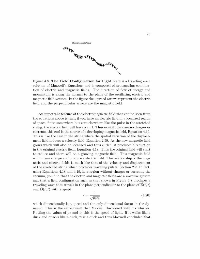
Figure 4.8: The Field Configuration for Light Light is a traveling wavesolution of Maxwell’s Equations and is composed of propagating combina-tion of electric and magnetic fields. The direction of flow of energy andmomentum is along the normal to the plane of the oscillating electric andmagnetic field vectors. In the figure the upward arrows represent the electricfield and the perpendicular arrows are the magnetic field.

An important feature of the electromagnetic field that can be seen fromthe equations above is that, if you have an electric field in a localized regionof space, finite somewhere but zero elsewhere like the pulse in the stretchedstring, the electric field will have a curl. Thus even if there are no charges orcurrents, this curl is the source of a developing magnetic field, Equation 4.19.This is like the case in the string where the spatial variation of the displace-ment field induces a velocity field, Equation 2.59. As the new magnetic fieldgrows which will also be localized and thus curled, it produces a reductionin the original electric field, Equation 4.18. Thus the original field will startto reduce and there will be a growing magnetic field. This magnetic fieldwill in turn change and produce a electric field. The relationship of the mag-netic and electric fields is much like that of the velocity and displacementof the stretched string which produces traveling pulses, Section 2.2. In fact,using Equations 4.18 and 4.19, in a region without charges or currents, thevacuum, you find that the electric and magnetic fields are a wavelike systemand that a field configuration such as that shown in Figure 4.8 produces atraveling wave that travels in the plane perpendicular to the plane of �E(�r, t)and �B(�r, t) with a speed

c =1

√µ0�0

(4.20)

which dimensionally is a speed and the only dimensional factor in the dy-namic. This is the same result that Maxwell discovered with his whirlies.Putting the values of µ0 and �0 this is the speed of light. If it walks like aduck and quacks like a duck, it is a duck and thus Maxwell concluded that

74 CHAPTER 4. INTRODUCTION TO MAXWELL’S THEORY

light is the traveling wave solutions to the equations of electromagnetism.Actually, we now reverse the process and assign a value to the speed oflight and use the measured definition of the second to allow the definitionof the meter and define µ0 and �0 to be consistent with Equation 4.20,see [Gleeson Modern Physics ].

It is important to realize that like in the stretched string which has only atransverse displacement and transverse velocity, the �E(�r, t) and �B(�r, t) fieldsare not traveling but only the disturbance – changes in the field configurationare. It is also important to realize that the velocity of the disturbance doesnot depend on the field configuration. It only depends on the dynamicof the field, Equation 4.20. Another way that this is often stated is thatthe velocity of propagation is a function only of the medium. Since theelectromagnetic field operates in the vacuum of space, it is the propertiesof the vacuum that determine the speed with which light propagates. Adifference for the electromagnetic travelers from the travelers of the field ofthe stretched string is that in the string any distortion will produce simplyrelated travelers but for the electromagnetic field there are configurations ofthe field that do not have simply related travelers.

We now understand what the amplitude that was invented by Youngand Fresnel to describe the phenomena of the interference and diffractionof light, see my notes [Gleeson Modern Physics ]. The amplitude is thetraveling waves solutions of the electric and magnetic fields.