LECTURE 1:

INTRODUCTION TO MARKOV

MODELS

OUTLINE

Markov model

Hidden Markov model (HMM)

Example: dice & coins

Example: recognizing eating activities

MOTIVATION

MARKOV CHAIN

What

is

are

the

next

word

at end

of

this

sentence

paragraph

line

P

P

P

P

P

P

P P

P

P

P

P

P

P

0.6

0.05

0.05

P

P P

message

0.3

P

P

MARKOV CHAIN: WEATHER EXAMPLE

Design a Markov Chain to predict the weather of tomorrow using previous information of the past days.

Our model has only 3 states: 𝑆 = 𝑆1, 𝑆2, 𝑆3 , and the name of each state is 𝑆1 = 𝑆𝑢𝑛𝑛𝑦 , 𝑆2 = 𝑅𝑎𝑖𝑛𝑦, 𝑆3 = 𝐶𝑙𝑜𝑢𝑑𝑦.

To establish the transition probabilities relationship between states we will need to collect data.

Assume the data produces the following transition

probabilities:

𝑃 𝑆𝑢𝑛𝑛𝑦 𝑆𝑢𝑛𝑛𝑦 = 0.8 𝑃 𝑅𝑎𝑖𝑛𝑦 𝑆𝑢𝑛𝑛𝑦 = 0.05 𝑃 𝐶𝑙𝑜𝑢𝑑𝑦 𝑆𝑢𝑛𝑛𝑦 = 0.15

𝑃 𝑆𝑢𝑛𝑛𝑦 𝑅𝑎𝑖𝑛𝑦 = 0.2 𝑃 𝑅𝑎𝑖𝑛𝑦 𝑅𝑎𝑖𝑛𝑦 = 0.6 𝑃 𝐶𝑙𝑜𝑢𝑑𝑦𝑦 𝑅𝑎𝑖𝑛𝑦 = 0.2

𝑃 𝑆𝑢𝑛𝑛𝑦 𝐶𝑙𝑜𝑢𝑑𝑦 = 0.2 𝑃 𝑅𝑎𝑖𝑛𝑦 𝐶𝑙𝑜𝑢𝑑𝑦 = 0.3 𝑃 𝐶𝑙𝑜𝑢𝑑𝑦 𝐶𝑙𝑜𝑢𝑑𝑦 = 0.5

1

1

1

Let’s say we have a sequence: Sunny, Rainy, Cloudy, Cloudy, Sunny, Sunny, Sunny, Rainy, ….; so, in a day we can be in any of the three states.

We can use the following state sequence notation: 𝑞1, 𝑞2, 𝑞3, 𝑞4, 𝑞5, … . ., where 𝑞𝑖 𝜖 {𝑆𝑢𝑛𝑛𝑦, 𝑅𝑎𝑖𝑛𝑦, 𝐶𝑙𝑜𝑢𝑑𝑦}.

In order to compute the probability of tomorrow’s weather we can use the Markov property:

𝑃 𝑞1, … , 𝑞𝑛 = 𝑃(𝑞𝑖|𝑞𝑖−1)

𝑛

𝑖=1

Exercise 1: Given that today is Sunny, what’s the probability that

tomorrow is Sunny and the next day Rainy?

𝑃 𝑞2, 𝑞3 𝑞1 = 𝑃 𝑞2 𝑞1 𝑃 𝑞3 𝑞1, 𝑞2

= 𝑃 𝑞2 𝑞1 𝑃 𝑞3 𝑞2

= 𝑃 𝑆𝑢𝑛𝑛𝑦 𝑆𝑢𝑛𝑛𝑦 𝑃 𝑅𝑎𝑖𝑛𝑦 𝑆𝑢𝑛𝑛𝑦

= 0.8 (0.05)

= 0.04

Exercise 2: Assume that yesterday’s weather was Rainy, and today is

Cloudy, what is the probability that tomorrow will be Sunny?

𝑃(𝑞3|𝑞1, 𝑞2) = 𝑃 𝑞3 𝑞2

= 𝑃 𝑆𝑢𝑛𝑛𝑦 𝐶𝑙𝑜𝑢𝑑𝑦

= 0.2

WHAT IS A MARKOV MODEL?

A Markov Model is a stochastic model which models temporal or sequential data, i.e., data that are ordered.

It provides a way to model the dependencies of current information (e.g. weather) with previous information.

It is composed of states, transition scheme between states, and emission of outputs (discrete or continuous).

Several goals can be accomplished by using Markov models:

Learn statistics of sequential data.

Do prediction or estimation.

Recognize patterns.

A Hidden Markov Model, is a stochastic model where

the states of the model are hidden. Each state can emit

an output which is observed.

Imagine: You were locked in a room for several days

and you were asked about the weather outside. The

only piece of evidence you have is whether the person

who comes into the room bringing your daily meal is

carrying an umbrella or not.

What is hidden? Sunny, Rainy, Cloudy

What can you observe? Umbrella or Not

WHAT IS A HIDDEN MARKOV MODEL

(HMM)?

MARKOV CHAIN VS. HMM

Markov Chain:

HMM:

U = Umbrella

NU = Not Umbrella

Let’s assume that 𝑡 days had passed. Therefore, we

will have an observation sequence O = {𝑜1, … , 𝑜𝑡} , where 𝑜𝑖 𝜖 𝑈𝑚𝑏𝑟𝑒𝑙𝑙𝑎, 𝑁𝑜𝑡 𝑈𝑚𝑏𝑟𝑒𝑙𝑙𝑎 .

Each observation comes from an unknown state.

Therefore, we will also have an unknown sequence

𝑄 = 𝑞1, … , 𝑞𝑡 , where 𝑞𝑖 𝜖 𝑆𝑢𝑛𝑛𝑦, 𝑅𝑎𝑖𝑛𝑦, 𝐶𝑙𝑜𝑢𝑑𝑦 .

We would like to know: 𝑃(𝑞1, . . , 𝑞𝑡|𝑜1, … , 𝑜𝑡).

HMM MATHEMATICAL MODEL

From Bayes’ Theorem, we can obtain the probability

for a particular day as:

𝑃 𝑞𝑖 𝑜𝑖 = 𝑃 𝑜𝑖 𝑞𝑖 𝑃(𝑞𝑖)

𝑃(𝑜𝑖)

For a sequence of length 𝑡:

𝑃 𝑞1, … , 𝑞𝑡 𝑜1, … , 𝑜𝑡 = 𝑃 𝑜1, … , 𝑜𝑡 𝑞1, … , 𝑞𝑡 𝑃(𝑞1, … , 𝑞𝑡)

𝑃(𝑜1, … , 𝑜𝑡)

From the Markov property:

𝑃 𝑞1, … , 𝑞𝑡 = 𝑃(𝑞𝑖|𝑞𝑖−1)

𝑡

𝑖=1

Independent observations assumption:

𝑃 𝑜1, … , 𝑜𝑡 𝑞1, … , 𝑞𝑡 = 𝑃(𝑜𝑖|𝑞𝑖)

𝑡

𝑖=1

Thus:

𝑃 𝑞1, … , 𝑞𝑡 𝑜1, … , 𝑜𝑡 ∝ 𝑃(𝑜𝑖|𝑞𝑖)

𝑡

𝑖=1

𝑃(𝑞𝑖|𝑞𝑖−1)

𝑡

𝑖=1

HMM Parameters:

• Transition probabilities 𝑃(𝑞𝑖|𝑞𝑖−1) • Emission probabilities 𝑃(𝑜𝑖|𝑞𝑖) • Initial state probabilities 𝑃(𝑞𝑖)

HMM PARAMETERS

A HMM is governed by the following parameters:

λ = {𝐴, 𝐵, 𝜋}

State-transition probability matrix 𝐴

Emission/Observation/State Conditional Output

probabilities 𝐵

Initial (prior) state probabilities 𝜋

Determine the fixed number of states (𝑁):

𝑆 = 𝑠1, … , 𝑠𝑁

State-transition probability matrix:

A =

𝑎11𝑎21...𝑎𝑁1

𝑎12𝑎23...𝑎𝑁2

.

.

.

.

.

.

.

.

.

.

. .

𝑎1𝑁𝑎2𝑁...𝑎𝑁𝑁

𝑎𝑖𝑗 = 𝑃(𝑞𝑡 = 𝑠𝑗 |𝑞𝑡−1 = 𝑠𝑖), 1 ≤ 𝑖, 𝑗 ≤ 𝑁

𝑎𝑖𝑗𝑁𝑗=1 = 1 (Each row/Outgoing arrows)

𝑎𝑖𝑗 → 𝑇𝑟𝑎𝑛𝑠𝑖𝑠𝑖𝑡𝑜𝑛 𝑝𝑟𝑜𝑏𝑎𝑏𝑖𝑙𝑖𝑡𝑦 𝑓𝑟𝑜𝑚 𝑠𝑡𝑎𝑡𝑒 𝑠𝑖 𝑡𝑜 𝑠𝑗

𝑠𝑖 𝑠𝑗

𝑎𝑖𝑗

𝑎𝑖𝑗 ≥ 0

Emission probabilities: A state will generate an

observation (output), but a decision must be taken

according on how to model the output, i.e., as discrete

or continuous.

Discrete outputs are modeled using pmfs.

Continuous outputs are modeled using pdfs.

Discrete Emission Probabilities:

𝐵 =

𝑏1(𝑣1)𝑏2(𝑣1)...𝑏𝑁(𝑣1)

𝑏1(𝑣2)𝑏2(𝑣2)...𝑏𝑁(𝑣2)

.

.

.

.

.

.

. .

.

.

.

𝑏1(𝑣𝑊)𝑏2(𝑣𝑊)...

𝑏𝑁(𝑣𝑊)

𝑏𝑖 𝑣𝑘 = 𝑃 𝑜𝑡 = 𝑣𝑘 𝑞𝑡 = 𝑠𝑖 , 1 ≤ 𝑘 ≤ 𝑊

Observation Set: 𝑉 = {𝑣1, … , 𝑣𝑊}

𝑠𝑖

𝑣1

𝑣2 𝑣𝑊

…

𝑏1 𝑣1

𝑏1 𝑣2 𝑏1 𝑣𝑊

Initial (prior) probabilities: these are the probabilities

of starting the observation sequence in state 𝑞𝑖 .

𝜋 =

𝜋1𝜋2...𝜋𝑁

𝜋𝑖 = 𝑃 𝑞1 = 𝑠𝑖 , 1 ≤ 𝑖 ≤ 𝑁

𝜋𝑖 = 1

𝑁

𝑖=1

HMM EXAMPLE: COINS & DICE

𝑃 𝐻 𝑅𝑒𝑑 𝐶𝑜𝑖𝑛 = 0.9

𝑃 𝑇 𝑅𝑒𝑑 𝐶𝑜𝑖𝑛 = 0.1

𝑃 𝐻 𝐺𝑟𝑒𝑒𝑛 𝐶𝑜𝑖𝑛 = 0.95

𝑃 𝑇 𝐺𝑟𝑒𝑒𝑛 𝐶𝑜𝑖𝑛 = 0.05

𝑂𝑢𝑡𝑝𝑢𝑡𝑠 = {1, 2, 3, 4, 5, 6} 𝑂𝑢𝑡𝑝𝑢𝑡𝑠 = {1, 1, 1, 1, 1, 1, 1, 2, 3, 4, 5, 6}

http://www.mathworks.com/help/stats/hidden-markov-models-hmm.html

HMM EXAMPLE: COINS & DICE

http://www.mathworks.com/help/stats/hidden-markov-models-hmm.html

State1

Red Die

(6 sides)

State2

Green

Die

(12 sides)

1

2

3

4 5 6 1

1

1

1

1 1 1 2 3

4

6

5

𝑃 𝐻 𝑅𝑒𝑑 𝐶𝑜𝑖𝑛 = 0.9 𝑃 𝑇 𝑅𝑒𝑑 𝐶𝑜𝑖𝑛 = 0.1

𝑃 𝑇 𝐺𝑟𝑒𝑒𝑛 𝐶𝑜𝑖𝑛 = 0.05

𝑃 𝐻 𝐺𝑟𝑒𝑒𝑛 𝐶𝑜𝑖𝑛 = 0.95

𝐴 = 0.90.05 0.10.95

𝜋 = 10

HMM EXAMPLE: COINS & DICE

0 1 2 3 4 5 6 70

0.02

0.04

0.06

0.08

0.1

0.12

0.14

0.16

0.18

0.2

Red Die Outcome

Pro

baili

ty

0 1 2 3 4 5 6 70

0.1

0.2

0.3

0.4

0.5

0.6

Green Die Outcome

Pro

baili

ty

𝑏1 𝑜𝑡 = {1

6,1

6,1

6,1

6,1

6,1

6}

𝑏2 𝑜𝑡 = {7

12,1

12,1

12,1

12,1

12,1

12}

HMM EXAMPLE: COINS & DICE

𝐵 =

1

67

12

1

6

1

12

1

61

12

1

61

12

1

61

12

1

6

1

12

http://www.mathworks.com/help/stats/hidden-markov-models-hmm.html

State1

Red Die

(6 sides)

State2

Green

Die

(12 sides)

1

2

3

4 5 6 1

1

1

1

1 1 1 2 3

4

6

5

𝑃 𝐻 𝑅𝑒𝑑 𝐶𝑜𝑖𝑛 = 0.9 𝑃 𝑇 𝑅𝑒𝑑 𝐶𝑜𝑖𝑛 = 0.1

𝑃 𝑇 𝐺𝑟𝑒𝑒𝑛 𝐶𝑜𝑖𝑛 = 0.05

𝑃 𝐻 𝐺𝑟𝑒𝑒𝑛 𝐶𝑜𝑖𝑛 = 0.95

𝐴 = 0.90.05 0.10.95

𝜋 = 10

HMM TO CLASSIFY WRIST MOTIONS

RELATED TO EATING ACTIVITIES

Wrist Motion:

Bite

273 Participants

Drink

Rest

?

THE “LANGUAGE”

DATA

Word p006 p098 p215 Total

Rest 24 44 21 87

Utensiling 21 37 16 74

Bite 29 44 18 91

Drink 5 15 4 24

DATA SEQUENCE:

50 100 150 200 250

rest

bite

utensiling

drink

p006 p098 p215

Sequence

Sta

tes

Training Data

A, 𝜋:

State 1

Rest

State 2

Bite

Sate 4

Drink Sate 3

Utensiling

0.26

0.42

0.24 0.42

0.04 0.13

0.72

0.29

0.00

0.38

0.11

0.50

0.21

0.16

0.08

0.04

𝜋 =

0.320.330.260.09

GMM GMM

GMM

GMM

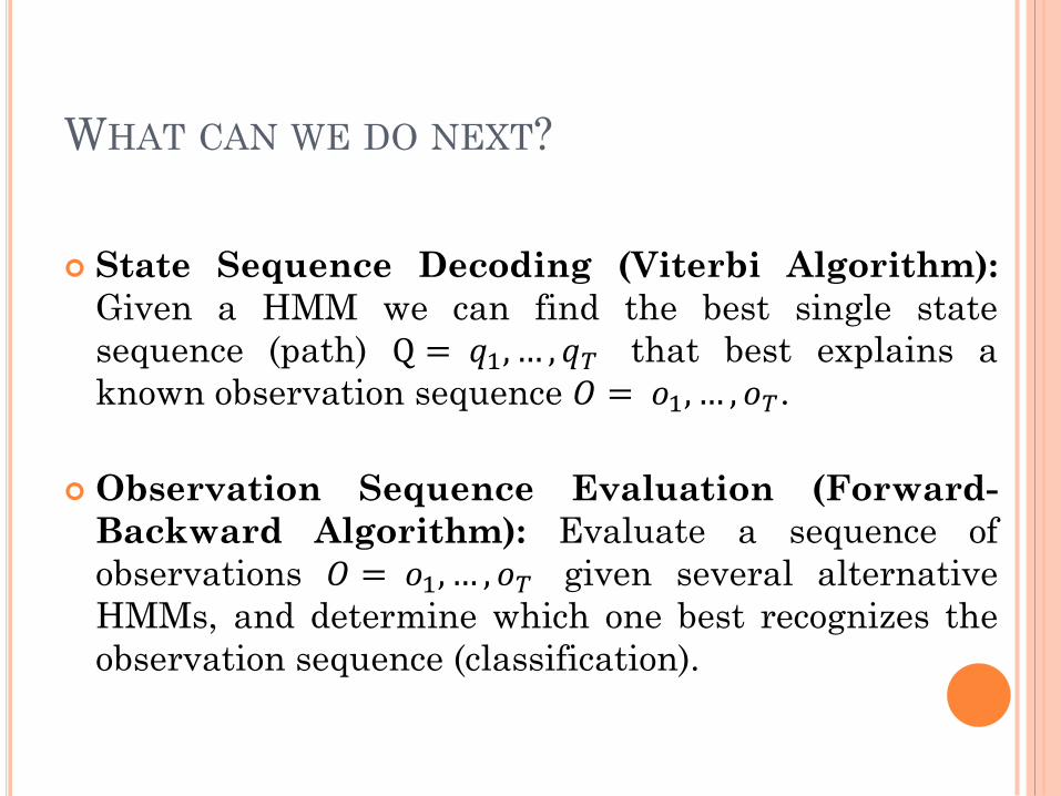
WHAT CAN WE DO NEXT?

State Sequence Decoding (Viterbi Algorithm):

Given a HMM we can find the best single state

sequence (path) Q = 𝑞1, … , 𝑞𝑇 that best explains a

known observation sequence 𝑂 = 𝑜1, … , 𝑜𝑇.

Observation Sequence Evaluation (Forward-

Backward Algorithm): Evaluate a sequence of

observations 𝑂 = 𝑜1, … , 𝑜𝑇 given several alternative

HMMs, and determine which one best recognizes the

observation sequence (classification).

REFERENCES

Rabiner, L.R.; , "A tutorial on hidden Markov models and selected applications in speech

recognition," Proceedings of the IEEE , vol.77, no.2, pp.257-286, Feb 1989

John R. Deller, John, and John H. L. Hansen. “Discrete-Time Processing of Speech Signals”. Prentice Hall, New

Jersey, 1987.

Barbara Resch (modified Erhard and Car Line Rank and Mathew Magimai-doss); “Hidden Markov Models A

Tutorial for the Course Computational Intelligence.”

Henry Stark and John W. Woods. “Probability and Random Processes with Applications to Signal Processing

(3rd Edition).” Prentice Hall, 3 edition, August 2001.

HTKBook: http://htk.eng.cam.ac.uk/docs/docs.shtml