Introduction to Malliavin calculus andApplications to Finance

Part I

Giulia Di Nunno

Finance and Insurance,Stochastic Analysis and Practical Methods

Spring SchoolMarie Curie ITN - Jena 2009

IntroductionThe mathematical theory now known as Malliavin calculus was firstintroduced by Paul Malliavin in 1978, as an infinite-dimensionalintegration by parts technique. The purpose of this calculus was to proveresults about the smoothness of densities of solutions of stochasticdifferential equations driven by Brownian motion. For several years thiswas the only known application.

In 1984, Ocone obtained an explicit interpretation of the Clarkrepresentation formula in terms of the Malliavin derivative (Clark-Oconeformula). In 1991 Ocone and Karatzas applied this result to finance:They proved that the Clark-Ocone formula can be used to obtain explicitformulae for replicating portfolios of contingent claims in completemarkets.

Since then Malliavin calculus has been applied in various domains within

finance and outside of it. In the meanwhile the very potentials in

applications created the need for an extension of the calculus to other

types of noise than Brownian motion.

PROGRAMPART I:

I Elements of Malliavin calculus for Brownian motion

I Clark-Ocone formula and hedging in complete markets

I Sensitivity analysis: the Greek delta

PART II:

I Levy processes and Poisson random measures

I Elements of Malliavin calculus for compensated Poisson randommeasures

I Minimal variance hedging in incomplete markets

PART III:

I Information, anticipative calculus and stochastic control

I Optimal portfolio selection and information

PART I

1. Elements of Malliavin calculus for Brownian motion• Iterated Ito integrals and Hermite polynomials• Wiener-Ito chaos expansions• Skorohod integral• Malliavin derivative• Fundamental rules of calculus

2. Clark-Ocone formula and hedging in complete markets• Clark-Ocone formula• A Black-Scholes type market model• Hedging• Hedging of Markovian setting: ∆-hedging

3. Sensitivity analysis: the Greeks• Computation of the Greeks: the ∆

References

1. Elements of Malliavin calculus for Brownian motion

We choose to introduce the operators Malliavin derivative and Skorohodintegral via chaos expansions. Other, basically equivalent, approach is touse directional derivatives on the Wiener space, see e.g. Da Prato(2007), Malliavin (1997), Nualart (2006), Sanz-Sole (2005).

Let W (t) = W (ω, t), ω ∈ Ω, t ∈ [0,T ] (T > 0), be a Brownian motionon the complete probability space (Ω,F ,P) such that W (0) = 0 P−a.s.For any t, let Ft be the σ-algebra generated by W (s), 0 ≤ s ≤ t,augmented by all the P-zero measure events. The resulting (continuous)filtration is denoted

F = Ft , t ≥ 0 .

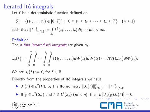
Iterated Ito integralsLet f be a deterministic function defined on

Sn = (t1, . . . , tn) ∈ [0,T ]n : 0 ≤ t1 ≤ t2 ≤ · · · ≤ tn ≤ T (n ≥ 1)

such that ‖f ‖2L2(Sn) :=

∫Sn

f 2(t1, . . . , tn)dt1 · · · dtn <∞.

DefinitionThe n-fold iterated Ito integrals are given by:

Jn(f ) :=

T∫0

tn∫0

· · ·t3∫

0

t2∫0

f (t1, . . . , tn)dW (t1)dW (t2) · · · dW (tn−1)dW (tn).

We set J0(f ) := f , for f ∈ R.

Directly from the properties of Ito integrals we have:

I Jn(f ) ∈ L2(P), by the Ito isometry ‖Jn(f )‖2L2(P) = ‖f ‖2

L2(Sn).

I If g ∈ L2(Sm) and f ∈ L2(Sn) (m < n), then E[Jm(g)Jn(f )

]= 0.

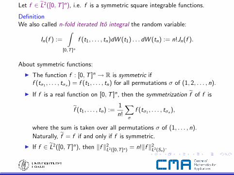
Let f ∈ L2([0,T ]n), i.e. f is a symmetric square integrable functions.

DefinitionWe also called n-fold iterated Ito integral the random variable:

In(f ) :=

∫[0,T ]n

f (t1, . . . , tn)dW (t1) . . . dW (tn) := n!Jn(f ).

About symmetric functions:

I The function f : [0,T ]n → R is symmetric iff (tσ1 , . . . , tσn ) = f (t1, . . . , tn) for all permutations σ of (1, 2, . . . , n).

I If f is a real function on [0,T ]n, then the symmetrization f of f is

f (t1, . . . , tn) :=1

n!

∑σ

f (tσ1 , . . . , tσn ),

where the sum is taken over all permutations σ of (1, . . . , n).

Naturally, f = f if and only if f is symmetric.

I If f ∈ L2([0,T ]n), then ‖f ‖2L2([0,T ]n) = n!‖f ‖2

L2(Sn).

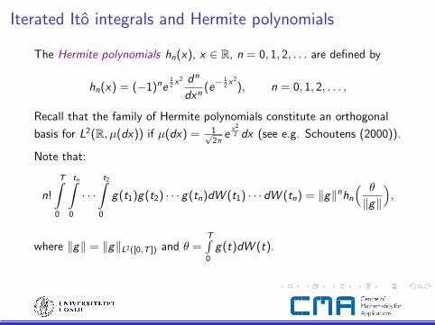
Iterated Ito integrals and Hermite polynomials

The Hermite polynomials hn(x), x ∈ R, n = 0, 1, 2, . . . are defined by

hn(x) = (−1)ne12 x2 dn

dxn(e− 1

2 x2

), n = 0, 1, 2, . . . ,

Recall that the family of Hermite polynomials constitute an orthogonal

basis for L2(R, µ(dx)) if µ(dx) = 1√2π

ex2

2 dx (see e.g. Schoutens (2000)).

Note that:

n!

T∫0

tn∫0

· · ·t2∫

0

g(t1)g(t2) · · · g(tn)dW (t1) · · · dW (tn) = ‖g‖nhn

( θ

‖g‖

),

where ‖g‖ = ‖g‖L2([0,T ]) and θ =T∫0

g(t)dW (t).

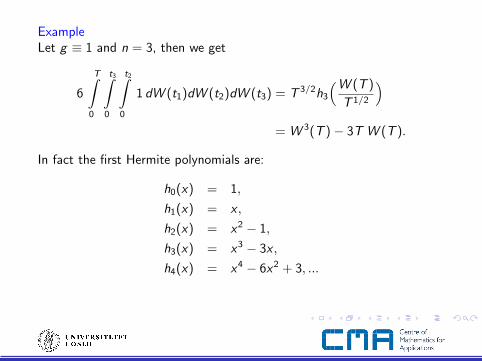
ExampleLet g ≡ 1 and n = 3, then we get

6

T∫0

t3∫0

t2∫0

1 dW (t1)dW (t2)dW (t3) = T 3/2h3

(W (T )

T 1/2

)= W 3(T )− 3T W (T ).

In fact the first Hermite polynomials are:

h0(x) = 1,

h1(x) = x ,

h2(x) = x2 − 1,

h3(x) = x3 − 3x ,

h4(x) = x4 − 6x2 + 3, ...

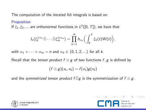
The computation of the iterated Ito integrals is based on:

PropositionIf ξ1, ξ2, ... are orthonormal functions in L2([0,T ]), we have that

In(ξ⊗α1

1 ⊗ · · · ⊗ξ⊗αmm

)=

m∏k=1

hαk

(∫ T

0

ξk (t)W (t)),

with α1 + · · ·+ αm = n and αk ∈ 0, 1, 2, ... for all k .

Recall that the tensor product f ⊗ g of two functions f , g is defined by

(f ⊗ g)(x1, x2) = f (x1)g(x2)

and the symmetrized tensor product f ⊗g is the symmetrization of f ⊗ g .

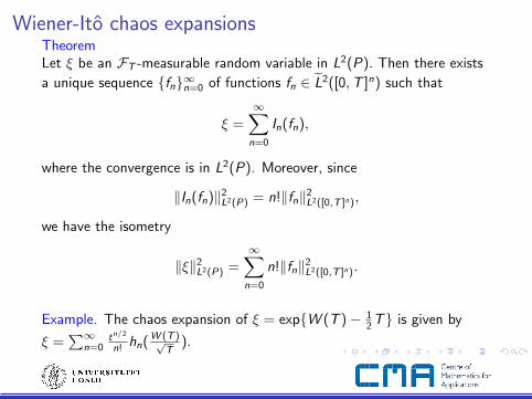
Wiener-Ito chaos expansionsTheoremLet ξ be an FT -measurable random variable in L2(P). Then there exists

a unique sequence fn∞n=0 of functions fn ∈ L2([0,T ]n) such that

ξ =∞∑

n=0

In(fn),

where the convergence is in L2(P). Moreover, since

‖In(fn)‖2L2(P) = n!‖fn‖2

L2([0,T ]n),

we have the isometry

‖ξ‖2L2(P) =

∞∑n=0

n!‖fn‖2L2([0,T ]n).

Example. The chaos expansion of ξ = expW (T )− 12 T is given by

ξ =∑∞

n=0tn/2

n! hn( W (T )√T

).

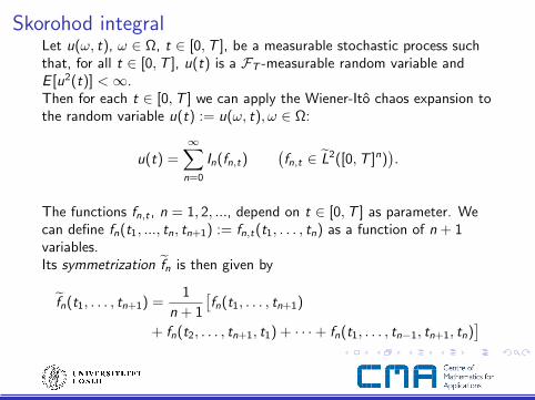
Skorohod integralLet u(ω, t), ω ∈ Ω, t ∈ [0,T ], be a measurable stochastic process suchthat, for all t ∈ [0,T ], u(t) is a FT -measurable random variable andE [u2(t)] <∞.Then for each t ∈ [0,T ] we can apply the Wiener-Ito chaos expansion tothe random variable u(t) := u(ω, t), ω ∈ Ω:

u(t) =∞∑

n=0

In(fn,t)(fn,t ∈ L2([0,T ]n)

).

The functions fn,t , n = 1, 2, ..., depend on t ∈ [0,T ] as parameter. Wecan define fn(t1, ..., tn, tn+1) := fn,t(t1, . . . , tn) as a function of n + 1variables.Its symmetrization fn is then given by

fn(t1, . . . , tn+1) =1

n + 1

[fn(t1, . . . , tn+1)

+ fn(t2, . . . , tn+1, t1) + · · ·+ fn(t1, . . . , tn−1, tn+1, tn)]

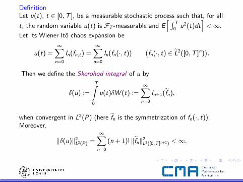
DefinitionLet u(t), t ∈ [0,T ], be a measurable stochastic process such that, for all

t, the random variable u(t) is FT -measurable and E[ ∫ T

0u2(t)dt

]<∞.

Let its Wiener-Ito chaos expansion be

u(t) =∞∑

n=0

In(fn,t) =∞∑

n=0

In(fn(·, t))(fn(·, t) ∈ L2([0,T ]n)

).

Then we define the Skorohod integral of u by

δ(u) :=

T∫0

u(t)δW (t) :=∞∑

n=0

In+1(fn),

when convergent in L2(P) (here fn is the symmetrization of fn(·, t)).Moreover,

‖δ(u)‖2L2(P) =

∞∑n=0

(n + 1)! ‖fn‖2L2([0,T ]n+1) <∞.

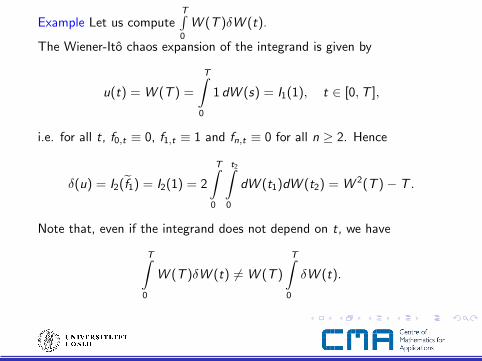
Example Let us computeT∫0

W (T )δW (t).

The Wiener-Ito chaos expansion of the integrand is given by

u(t) = W (T ) =

T∫0

1 dW (s) = I1(1), t ∈ [0,T ],

i.e. for all t, f0,t ≡ 0, f1,t ≡ 1 and fn,t ≡ 0 for all n ≥ 2. Hence

δ(u) = I2(f1) = I2(1) = 2

T∫0

t2∫0

dW (t1)dW (t2) = W 2(T )− T .

Note that, even if the integrand does not depend on t, we have

T∫0

W (T )δW (t) 6= W (T )

T∫0

δW (t).

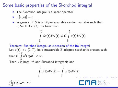
Some basic properties of the Skorohod integral

I The Skorohod integral is a linear operator

I E[δ(u)

]= 0

I In general, if G is an FT -measurable random variable such thatu,Gu ∈ Dom(δ), we have that

T∫0

Gu(t)δW (t) 6= G

T∫0

u(t)δW (t).

Theorem: Skorohod integral as extension of the Ito integralLet u(t), t ∈ [0,T ], be a measurable F-adapted stochastic process such

that E[ T∫

0

u2(t)dt]<∞.

Then u is both Ito and Skorohod integrable and

T∫0

u(t)δW (t) =

T∫0

u(t)dW (t).

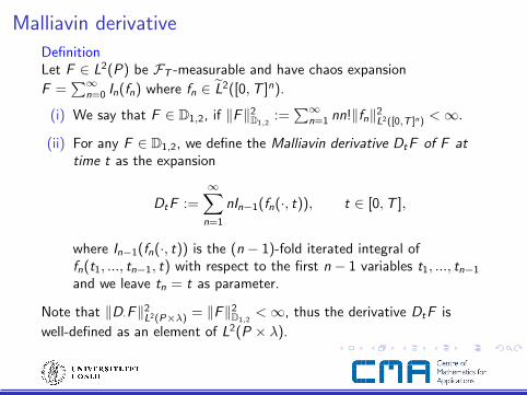
Malliavin derivative

DefinitionLet F ∈ L2(P) be FT -measurable and have chaos expansion

F =∑∞

n=0 In(fn) where fn ∈ L2([0,T ]n).

(i) We say that F ∈ D1,2, if ‖F‖2D1,2

:=∑∞

n=1 nn!‖fn‖2L2([0,T ]n) <∞.

(ii) For any F ∈ D1,2, we define the Malliavin derivative DtF of F attime t as the expansion

DtF :=∞∑

n=1

nIn−1(fn(·, t)), t ∈ [0,T ],

where In−1(fn(·, t)) is the (n − 1)-fold iterated integral offn(t1, ..., tn−1, t) with respect to the first n − 1 variables t1, ..., tn−1

and we leave tn = t as parameter.

Note that ‖D·F‖2L2(P×λ) = ‖F‖2

D1,2<∞, thus the derivative DtF is

well-defined as an element of L2(P × λ).

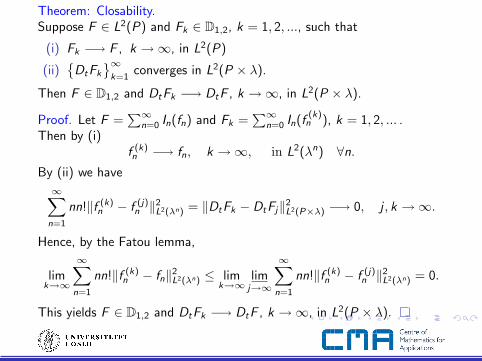
Theorem: Closability.Suppose F ∈ L2(P) and Fk ∈ D1,2, k = 1, 2, ..., such that

(i) Fk −→ F , k →∞, in L2(P)

(ii)

DtFk

∞k=1

converges in L2(P × λ).

Then F ∈ D1,2 and DtFk −→ DtF , k →∞, in L2(P × λ).

Proof. Let F =∑∞

n=0 In(fn) and Fk =∑∞

n=0 In(f(k)

n ), k = 1, 2, ... .Then by (i)

f (k)n −→ fn, k →∞, in L2(λn) ∀n.

By (ii) we have

∞∑n=1

nn!‖f (k)n − f (j)

n ‖2L2(λn) = ‖DtFk − DtFj‖2

L2(P×λ) −→ 0, j , k →∞.

Hence, by the Fatou lemma,

limk→∞

∞∑n=1

nn!‖f (k)n − fn‖2

L2(λn) ≤ limk→∞

limj→∞

∞∑n=1

nn!‖f (k)n − f (j)

n ‖2L2(λn) = 0.

This yields F ∈ D1,2 and DtFk −→ DtF , k →∞, in L2(P × λ).

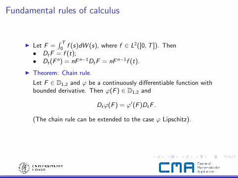
Fundamental rules of calculus

I Let F =∫ T

0f (s)dW (s), where f ∈ L2([0,T ]). Then

• DtF = f (t);• Dt(F n) = nF n−1DtF = nF n−1f (t).

I Theorem: Chain rule.

Let F ∈ D1,2 and ϕ be a continuously differentiable function withbounded derivative. Then ϕ(F ) ∈ D1,2 and

Dtϕ(F ) = ϕ′(F )DtF .

(The chain rule can be extended to the case ϕ Lipschitz).

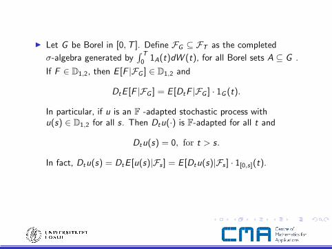
I Let G be Borel in [0,T ]. Define FG ⊆ FT as the completed

σ-algebra generated by∫ T

01A(t)dW (t), for all Borel sets A ⊆ G .

If F ∈ D1,2, then E [F |FG ] ∈ D1,2 and

DtE [F |FG ] = E [DtF |FG ] · 1G (t).

In particular, if u is an F -adapted stochastic process withu(s) ∈ D1,2 for all s. Then Dtu(·) is F-adapted for all t and

Dtu(s) = 0, for t > s.

In fact, Dtu(s) = DtE [u(s)|Fs ] = E [Dtu(s)|Fs ] · 1[0,s](t).

The Skorohod integral is the adjoint operator to the Malliavin derivative:

Theorem: Duality formulaLet F ∈ D1,2 be FT -measurable and let u(t), t ∈ [0,T ], be a Skorohodintegrable process. Then

E[F

∫ T

0

u(t)δW (t)]

= E[ ∫ T

0

u(t)DtF dt].

By the duality formula it is easy to see that the Skorohod integral is a

closed operator.

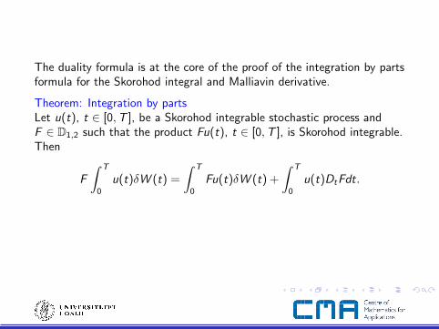
The duality formula is at the core of the proof of the integration by partsformula for the Skorohod integral and Malliavin derivative.

Theorem: Integration by partsLet u(t), t ∈ [0,T ], be a Skorohod integrable stochastic process andF ∈ D1,2 such that the product Fu(t), t ∈ [0,T ], is Skorohod integrable.Then

F

∫ T

0

u(t)δW (t) =

∫ T

0

Fu(t)δW (t) +

∫ T

0

u(t)DtFdt.

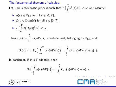
The fundamental theorem of calculus.

Let u be a stochastic process such that E[ T∫

0

u2(s)ds]<∞ and assume:

I u(s) ∈ D1,2 for all s ∈ [0,T ],

I Dtu ∈ Dom(δ) for all t ∈ [0,T ],

I E[ T∫

0

(δ(Dtu))2dt]<∞.

Then δ(u) :=T∫0

u(s)δW (s) is well-defined, belonging to D1,2, and

Dtδ(u) := Dt

(∫ T

0

u(s)δW (s))

=

T∫0

Dtu(s)δW (s) + u(t).

In particular, if u is F-adapted, then

Dt

( T∫0

u(s)dW (s))

=

T∫t

Dtu(s)dW (s) + u(t).

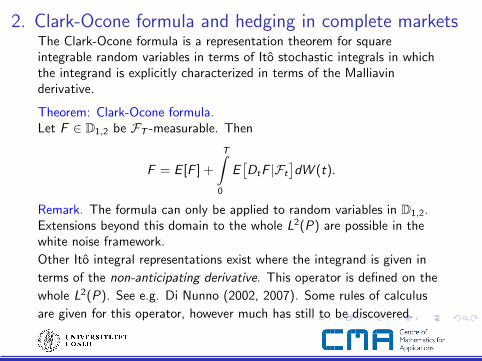
2. Clark-Ocone formula and hedging in complete marketsThe Clark-Ocone formula is a representation theorem for squareintegrable random variables in terms of Ito stochastic integrals in whichthe integrand is explicitly characterized in terms of the Malliavinderivative.

Theorem: Clark-Ocone formula.Let F ∈ D1,2 be FT -measurable. Then

F = E [F ] +

T∫0

E[DtF |Ft

]dW (t).

Remark. The formula can only be applied to random variables in D1,2.Extensions beyond this domain to the whole L2(P) are possible in thewhite noise framework.

Other Ito integral representations exist where the integrand is given in

terms of the non-anticipating derivative. This operator is defined on the

whole L2(P). See e.g. Di Nunno (2002, 2007). Some rules of calculus

are given for this operator, however much has still to be discovered.

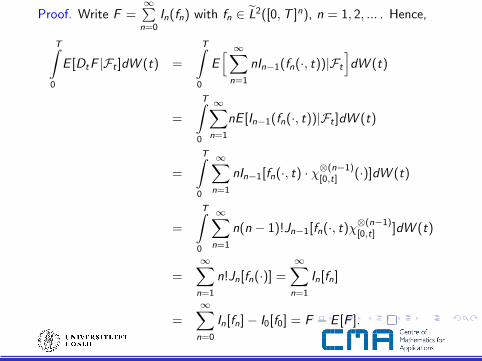
Proof. Write F =∞∑

n=0In(fn) with fn ∈ L2([0,T ]n), n = 1, 2, ... . Hence,

T∫0

E [DtF |Ft ]dW (t) =

T∫0

E[ ∞∑

n=1

nIn−1(fn(·, t))|Ft

]dW (t)

=

T∫0

∞∑n=1

nE [In−1(fn(·, t))|Ft ]dW (t)

=

T∫0

∞∑n=1

nIn−1[fn(·, t) · χ⊗(n−1)[0,t] (·)]dW (t)

=

T∫0

∞∑n=1

n(n − 1)!Jn−1[fn(·, t)χ⊗(n−1)[0,t] ]dW (t)

=∞∑

n=1

n!Jn[fn(·)] =∞∑

n=1

In[fn]

=∞∑

n=0

In[fn]− I0[f0] = F − E [F ].

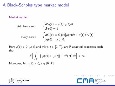
A Black-Scholes type market model

Market model.

risk free asset

dS0(t) = ρ(t)S0(t)dt

S0(0) = 1

risky asset

dS1(t) = S1(t)

[µ(t)dt + σ(t)dW (t)

]S1(0) = x > 0.

Here ρ(t) > 0, µ(t) and σ(t), t ∈ [0,T ], are F-adapted processes suchthat

E[ ∫ T

0

|ρ(t)|+ |µ(t)|+ σ2(t)

dt]<∞.

Moreover, let σ(t) 6= 0, t ∈ [0,T ].

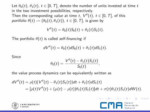
Let θ0(t), θ1(t), t ∈ [0,T ], denote the number of units invested at time tin the two investment possibilities, respectively.Then the corresponding value at time t, V θ(t), t ∈ [0,T ], of thisportfolio θ(t) := (θ0(t), θ1(t)), t ∈ [0,T ], is given by

V θ(t) = θ0(t)S0(t) + θ1(t)S1(t).

The portfolio θ(t) is called self-financing if

dV θ(t) = θ0(t)dS0(t) + θ1(t)dS1(t).

Since

θ0(t) =V θ(t)− θ1(t)S1(t)

S0(t),

the value process dynamics can be equivalently written as

dV θ(t) = ρ(t)(V θ(t)− θ1(t)S1(t))dt + θ1(t)dS1(t)

= [ρ(t)V θ(t) + (µ(t)− ρ(t))θ1(t)S1(t)]dt + σ(t)θ1(t)S1(t)dW (t).

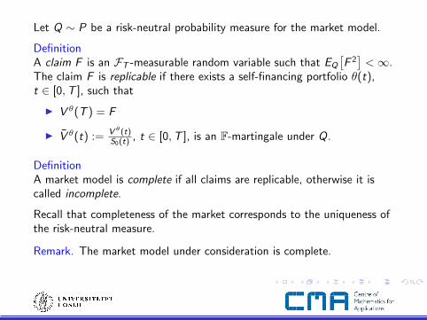
Let Q ∼ P be a risk-neutral probability measure for the market model.

DefinitionA claim F is an FT -measurable random variable such that EQ

[F 2]<∞.

The claim F is replicable if there exists a self-financing portfolio θ(t),t ∈ [0,T ], such that

I V θ(T ) = F

I V θ(t) := V θ(t)S0(t) , t ∈ [0,T ], is an F-martingale under Q.

DefinitionA market model is complete if all claims are replicable, otherwise it iscalled incomplete.

Recall that completeness of the market corresponds to the uniqueness ofthe risk-neutral measure.

Remark. The market model under consideration is complete.

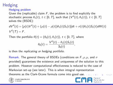
HedgingHedging problemGiven the (replicable) claim F , the problem is to find explicitly thestochastic process θ1(t), t ∈ [0,T ], such that (V θ(t), θ1(t)), t ∈ [0,T ]solves the (BSDE):

dV θ(t) = [ρ(t)V θ(t) + (µ(t)− ρ(t))θ1(t)S1(t)]dt + σ(t)θ1(t)S1(t)dW (t)

V θ(T ) = F .

Then the portfolio θ(t) = (θ0(t), θ1(t)), t ∈ [0,T ], where

θ0(t) =V θ(t)− θ1(t)S1(t)

S0(t),

is then the replicating or hedging portfolio.

Remark. The general theory of BSDEs (conditions on F , ρ, µ, and σ

provided) guarantees the existence and uniqueness of the solution to this

problem. However computational effectiveness is reduced to the case of

Markovian set-up (see later). This is when integral representation

theorems as the Clark-Ocone formula come into good use.

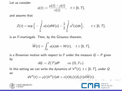
Let us consider

u(t) :=µ(t)− ρ(t)

σ(t), t ∈ [0,T ],

and assume that

Z (t) = exp−

t∫0

u(s)dW (s)− 1

2

t∫0

u2(s)ds, t ∈ [0,T ],

is an F-martingale. Then, by the Girsanov theorem,

W (t) =

∫ t

0

u(s)ds + W (t), t ∈ [0,T ],

is a Brownian motion with respect to F under the measure Q ∼ P givenby

dQ := Z (T )dP on (Ω,FT ).

In this setting we can write the dynamics of V θ(t), t ∈ [0,T ], under Qas:

dV θ(t) = ρ(t)V θ(t)dt + σ(t)θ1(t)S1(t)dW (t).

Thus the original BSDE under Q becomes

dV θ(t) :=d(S−1

0 (t) V θ(t))

=e−R t

0ρ(s)dsσ(t)θ1(t)S1(t)dW (t)

V θ(T ) = S−10 (T ) F = e−

R T0ρ(s)dsF =: G .

Hence,

G = V θ(0) +

∫ T

0

ϕ(t)dW (t)

whereϕ(t) := e−

R t0ρ(s)dsσ(t)θ1(t)S1(t).

The solution can be given by applying the Clark-Ocone formula with

respect to the Brownian motion W under Q.

However, there is need for carefulness!

Remark. The given Clark-Ocone formula is applicable to randomvariables G that are measurable with respect to the filtration generated

by the noise. If F is the (P ∼)Q- augmented filtration generated by W ,then we have that, in general,

Ft ⊂ Ft with Ft 6= Ft .

Need for a Clark-Ocone formula fitting this setting!

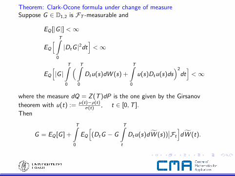
Theorem: Clark-Ocone formula under change of measureSuppose G ∈ D1,2 is FT -measurable and

EQ [|G |] <∞

EQ

[ T∫0

|DtG |2dt]<∞

EQ

[|G |

T∫0

( T∫0

Dtu(s)dW (s) +

T∫0

u(s)Dtu(s)ds)2

dt]<∞

where the measure dQ = Z (T )dP is the one given by the Girsanov

theorem with u(t) := µ(t)−ρ(t)σ(t) , t ∈ [0,T ].

Then

G = EQ [G ] +

T∫0

EQ

[(DtG − G

T∫t

Dtu(s)dW (s))∣∣Ft

]dW (t).

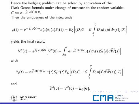
Hence the hedging problem can be solved by application of theClark-Ocone formula under change of measure to the random variable:

G := e−R T

0ρ(s)dsF .

Then the uniqueness of the integrands

ϕ(t) = e−R t

0ρ(s)dsσ(t)θ1(t)S1(t) = EQ

[(DtG − G

T∫t

Dtu(s)dW (s))|Ft

]yields the final result:

V θ(t) = eR t

0ρ(s)ds

[V θ(0) +

∫ t

0

e−R s

0ρ(r)drσ(s)θ1(s)S1(s)dW (s)

]with

θ1(t) = eR t

0ρ(s)dsσ−1(t)S−1

1 (t)EQ

[(DtG − G

T∫t

Dtu(s)dW (s))|Ft

]and

V θ(0) = V θ(0) = EQ [G ].

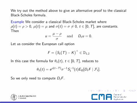
We try out the method above to give an alternative proof to the classicalBlack-Scholes formula.

Example We consider a classical Black-Scholes market whereρ(t) = ρ > 0, µ(t) = µ and σ(t) = σ 6= 0, t ∈ [0,T ], are constants.Then

u =µ− ρσ

and Dtu = 0.

Let us consider the European call option

F =(S1(T )− K

)+ ∈ D1,2

In this case the formula for θ1(t), t ∈ [0,T ], reduces to

θ1(t) = eρ(t−T )σ−1S−11 (t)EQ [DtF | Ft ].

So we only need to compute DtF .

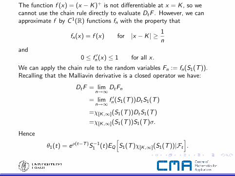
The function f (x) = (x − K )+ is not differentiable at x = K , so wecannot use the chain rule directly to evaluate DtF . However, we canapproximate f by C 1(R) functions fn with the property that

fn(x) = f (x) for |x − K | ≥ 1

n

and0 ≤ f ′n (x) ≤ 1 for all x .

We can apply the chain rule to the random variables Fn := fn(S1(T )).Recalling that the Malliavin derivative is a closed operator we have:

DtF = limn→∞

DtFn

= limn→∞

f ′n (S1(T ))DtS1(T )

=χ[K ,∞](S1(T ))DtS1(T )

=χ[K ,∞](S1(T ))S1(T )σ.

Hence

θ1(t) = eρ(t−T )S−11 (t)EQ

[S1(T )χ[K ,∞](S1(T ))|Ft

].

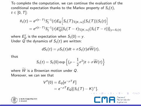
To complete the computation, we can continue the evaluation of theconditional expectation thanks to the Markov property of S1(t),t ∈ [0,T ]:

θ1(t) = eρ(t−T )S−11 (t)EQ

[S1(T )χ[K ,∞](S1(T ))|S1(t)

]= eρ(t−T )S−1

1 (t)E yQ [S1(T − t)χ[K ,∞](S1(T − t))]|y=S1(t)

where E yQ is the expectation when S1(0) = y .

Under Q the dynamics of S1(t) are written:

dS1(t) = ρS1(t)dt + σS1(t)dW (t),

thus

S1(t) = S1(0) exp

(ρ− 1

2σ2)t + σW (t)

where W is a Brownian motion under Q.Moreover, we can see that

V θ(0) = EQ [e−ρT F ]

= e−ρT EQ [(S1(T )− K )+].

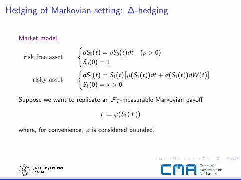
Hedging of Markovian setting: ∆-hedging

Market model.

risk free asset

dS0(t) = ρS0(t)dt (ρ > 0)

S0(0) = 1

risky asset

dS1(t) = S1(t)

[µ(S1(t))dt + σ(S1(t))dW (t)

]S1(0) = x > 0.

Suppose we want to replicate an FT -measurable Markovian payoff

F = ϕ(S1(T ))

where, for convenience, ϕ is considered bounded.

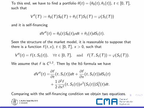
To this end, we have to find a portfolio θ(t) = (θ0(t), θ1(t)), t ∈ [0,T ],such that

V θ(T ) := θ0(T )S0(T ) + θ1(T )S1(T ) = ϕ(S1(T ))

and it is self-financing

dV θ(t) = θ0(t)S0(t)ρdt + θ1(t)dS1(t).

Seen the structure of the market model, it is reasonable to suppose thatthere is a function f (t, x), t ∈ [0,T ], x > 0, such that

V θ(t) = f (t,S1(t)), ∀t ∈ [0,T ], and f (T ,S1(T )) = ϕ(S1(T )).

We assume that f is C 1,2. Then by the Ito formula we have

dV θ(t) =∂f

∂t(t,S1(t))dt +

∂f

∂x(t,S1(t))dS1(t)

+1

2

∂2f

∂x2(t,S1(t))σ2(S1(t))S2

1 (t)dt.

Comparing with the self-financing condition we obtain two equations.

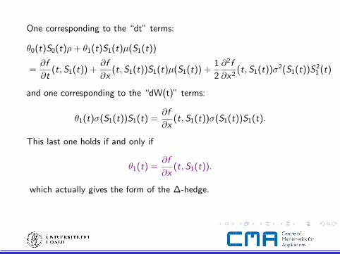
One corresponding to the “dt” terms:

θ0(t)S0(t)ρ+ θ1(t)S1(t)µ(S1(t))

=∂f

∂t(t,S1(t)) +

∂f

∂x(t,S1(t))S1(t)µ(S1(t)) +

1

2

∂2f

∂x2(t,S1(t))σ2(S1(t))S2

1 (t)

and one corresponding to the “dW(t)” terms:

θ1(t)σ(S1(t))S1(t) =∂f

∂x(t,S1(t))σ(S1(t))S1(t).

This last one holds if and only if

θ1(t) =∂f

∂x(t,S1(t)).

which actually gives the form of the ∆-hedge.

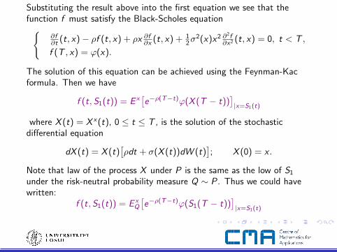
Substituting the result above into the first equation we see that thefunction f must satisfy the Black-Scholes equation

∂f∂t (t, x)− ρf (t, x) + ρx ∂f

∂x (t, x) + 12σ

2(x)x2 ∂2f∂x2 (t, x) = 0, t < T ,

f (T , x) = ϕ(x).

The solution of this equation can be achieved using the Feynman-Kacformula. Then we have

f (t,S1(t)) = E x[e−ρ(T−t)ϕ(X (T − t))

]|x=S1(t)

where X (t) = X x (t), 0 ≤ t ≤ T , is the solution of the stochasticdifferential equation

dX (t) = X (t)[ρdt + σ(X (t))dW (t)

]; X (0) = x .

Note that law of the process X under P is the same as the low of S1

under the risk-neutral probability measure Q ∼ P. Thus we could havewritten:

f (t,S1(t)) = E xQ

[e−ρ(T−t)ϕ(S1(T − t))

]|x=S1(t)

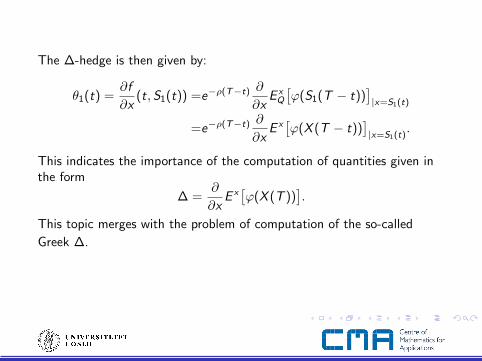
The ∆-hedge is then given by:

θ1(t) =∂f

∂x(t,S1(t)) =e−ρ(T−t) ∂

∂xE x

Q

[ϕ(S1(T − t))

]|x=S1(t)

=e−ρ(T−t) ∂

∂xE x[ϕ(X (T − t))

]|x=S1(t)

.

This indicates the importance of the computation of quantities given inthe form

∆ =∂

∂xE x[ϕ(X (T ))

].

This topic merges with the problem of computation of the so-called

Greek ∆.

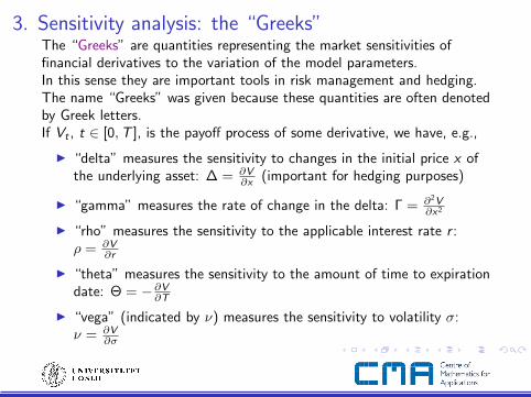
3. Sensitivity analysis: the “Greeks”The “Greeks” are quantities representing the market sensitivities offinancial derivatives to the variation of the model parameters.In this sense they are important tools in risk management and hedging.The name “Greeks” was given because these quantities are often denotedby Greek letters.If Vt , t ∈ [0,T ], is the payoff process of some derivative, we have, e.g.,

I “delta” measures the sensitivity to changes in the initial price x ofthe underlying asset: ∆ = ∂V

∂x (important for hedging purposes)

I “gamma” measures the rate of change in the delta: Γ = ∂2V∂x2

I “rho” measures the sensitivity to the applicable interest rate r :ρ = ∂V

∂r

I “theta” measures the sensitivity to the amount of time to expirationdate: Θ = −∂V

∂T

I “vega” (indicated by ν) measures the sensitivity to volatility σ:ν = ∂V

∂σ

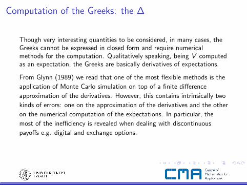
Computation of the Greeks: the ∆

Though very interesting quantities to be considered, in many cases, theGreeks cannot be expressed in closed form and require numericalmethods for the computation. Qualitatively speaking, being V computedas an expectation, the Greeks are basically derivatives of expectations.

From Glynn (1989) we read that one of the most flexible methods is the

application of Monte Carlo simulation on top of a finite difference

approximation of the derivatives. However, this contains intrinsically two

kinds of errors: one on the approximation of the derivatives and the other

on the numerical computation of the expectations. In particular, the

most of the inefficiency is revealed when dealing with discontinuous

payoffs e.g. digital and exchange options.

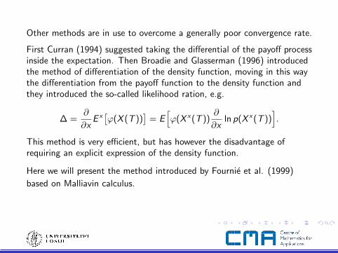
Other methods are in use to overcome a generally poor convergence rate.

First Curran (1994) suggested taking the differential of the payoff processinside the expectation. Then Broadie and Glasserman (1996) introducedthe method of differentiation of the density function, moving in this waythe differentiation from the payoff function to the density function andthey introduced the so-called likelihood ration, e.g.

∆ =∂

∂xE x[ϕ(X (T ))

]= E

[ϕ(X x (T ))

∂

∂xln p(X x (T ))

].

This method is very efficient, but has however the disadvantage ofrequiring an explicit expression of the density function.

Here we will present the method introduced by Fournie et al. (1999)

based on Malliavin calculus.

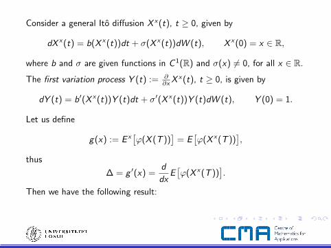
Consider a general Ito diffusion X x (t), t ≥ 0, given by

dX x (t) = b(X x (t))dt + σ(X x (t))dW (t), X x (0) = x ∈ R,

where b and σ are given functions in C 1(R) and σ(x) 6= 0, for all x ∈ R.

The first variation process Y (t) := ∂∂x X x (t), t ≥ 0, is given by

dY (t) = b′(X x (t))Y (t)dt + σ′(X x (t))Y (t)dW (t), Y (0) = 1.

Let us define

g(x) := E x[ϕ(X (T ))

]= E

[ϕ(X x (T ))

],

thus

∆ = g ′(x) =d

dxE[ϕ(X x (T ))

].

Then we have the following result:

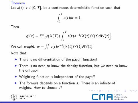
TheoremLet a(t), t ∈ [0,T ], be a continuous deterministic function such that∫ T

0

a(t)dt = 1.

Then

g ′(x) = E x[ϕ(X (T ))

∫ T

0

a(t)σ−1(X (t))Y (t)dW (t)].

We call weight: w =∫ T

0a(t)σ−1(X (t))Y (t)dW (t).

Note that:

I There is no differentiation of the payoff function!

I There is no need to know the density function, but we need to knowthe diffusion

I Weighting function is independent of the payoff

I The formula depends on a function a. There is an infinity ofweights. How to choose a?

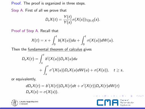
Proof. The proof is organized in three steps.

Step A. First of all we prove that

DsX (t) =Y (t)

Y (s)σ(X (s))χ[0,t](s).

Proof of Step A. Recall that

X (t) = x +

∫ t

0

b(X (u))du +

∫ t

0

σ(X (u))dW (u).

Then the fundamental theorem of calculus gives

DsX (t) =

∫ t

s

b′(X (u))DsX (u)du

+

∫ t

s

σ′(X (u))DsX (u)dW (u) + σ(X (s)), t ≥ s,

or equivalently,

dDsX (t) = b′(X (t))DsX (t)dt + σ′(X (t))DsX (t)dW (t)

DsX (s) = σ(X (s)).

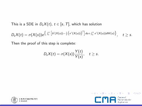
This is a SDE in DsX (t), t ∈ [s,T ], which has solution

DsX (t) = σ(X (s))e

R ts

[b′(X (u))− 1

2

(σ′(X (u))

)2]du+

R tsσ′(X (u))dW (u)

, t ≥ s.

Then the proof of this step is complete:

DsX (t) = σ(X (s))Y (t)

Y (s), t ≥ s.

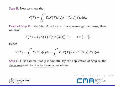
Step B. Now we show that

Y (T ) =

∫ T

0

DsX (T )a(s)σ−1(X (s))Y (s)ds,

Proof of Step B. Take Step A, with t = T and rearrange the terms, thenwe have

Y (T ) = DsX (T )Y (s)σ(X (s))−1, s ∈ [0,T ].

Hence

Y (T ) =

∫ T

0

Y (T )a(s)ds =

∫ T

0

DsX (T )a(s)σ−1(X (s))Y (s)ds.

Step C. First assume that ϕ is smooth. By the application of Step A, the

chain rule and the duality formula, we obtain

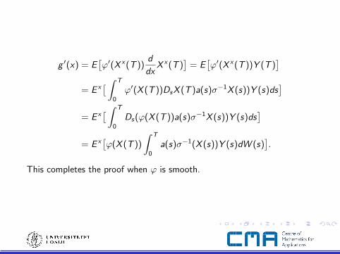
g ′(x) = E[ϕ′(X x (T ))

d

dxX x (T )

]= E

[ϕ′(X x (T ))Y (T )

]= E x

[ ∫ T

0

ϕ′(X (T ))DsX (T )a(s)σ−1X (s))Y (s)ds]

= E x[ ∫ T

0

Ds(ϕ(X (T ))a(s)σ−1X (s))Y (s)ds]

= E x[ϕ(X (T ))

∫ T

0

a(s)σ−1(X (s))Y (s)dW (s)].

This completes the proof when ϕ is smooth.

The general case is treated by approximation:

ϕm −→ ϕ, m→∞,

where ϕm are smooth functions bounded a.e. on [0,T ] and theconvergence is pointwise. Define

gm(x) := E x[ϕm(X (T ))

].

Then by Step B we have

g ′m(x) = E x[ϕm(X (T ))Λ

], m = 1, 2, ...,

where Λ =∫ T

0a(s)σ−1(X (s))Y (s)dW (s). Hence

limm→∞

g ′m(x) = E x[ϕ(X (T ))Λ

]=: h(x).

Thus

g(x) = limm→∞

gm(x) = limm→∞

gm(0) +

∫ x

0

g ′m(t)dt = g(0) +

∫ x

0

h(t)dt.

Then g is differentiable and g ′(x) = h(x) = E x[ϕ(X (T ))Λ

].

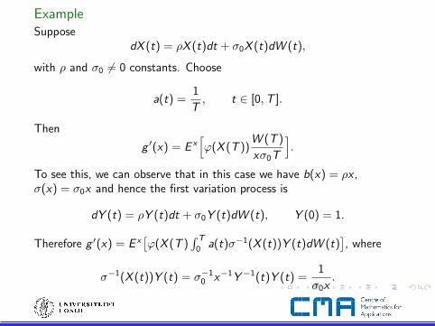
ExampleSuppose

dX (t) = ρX (t)dt + σ0X (t)dW (t),

with ρ and σ0 6= 0 constants. Choose

a(t) =1

T, t ∈ [0,T ].

Then

g ′(x) = E x[ϕ(X (T ))

W (T )

xσ0T

].

To see this, we can observe that in this case we have b(x) = ρx ,σ(x) = σ0x and hence the first variation process is

dY (t) = ρY (t)dt + σ0Y (t)dW (t), Y (0) = 1.

Therefore g ′(x) = E x[ϕ(X (T )

∫ T

0a(t)σ−1(X (t))Y (t)dW (t)

], where

σ−1(X (t))Y (t) = σ−10 x−1Y−1(t)Y (t) =

1

σ0x.

Other comments

I Avellaneda et al. (2000) also worked in the direction of moving thedifferentiation from the payoff function to the inclusion of aweighting function. They propose another way of finding theweighting function inspired by the Kullback-Leibler relative entropymaximization.

I Benhamou (2003) and related works studies how to characterizeand choose the weighs.

I His study indicates that the weights can be expressed asSkorohod integrals and one can introduce the concept of a“weighting function generator”.

I As for the choice of the weights, he focuses on the onesproviding the minimum variance of the random variable:ϕ(X (T )) · w .

I It turns out that the minimum variance weight is theconditional expectation of any wight with respect to X (T ).

I This result provides also the link with the likelihood ration inthe density method.

References

This presentation follows:

G. Di Nunno, B. Øksendal, and F. Proske, Malliavin Calculus for Levy Processes with Applications to Finance,Springer 2008.

References on the topic at the base of this presentation include:

M. Avellaned and R. Gamba, Conquering the Greeks in Monte Carlo. Proceedings of the First Bachelier Congress2001.

D.R. Bell, The Malliavin Calculus. Longman Scientific & Technical, 1987.

E. Benhamou, Optimal Malliavin weighting function for the computation of the Greeks, Mathematical Finance, 13(2003), 37-53.

M. Broadie and P. Glasserman, Estimating security price derivatives using simulation, Mgmt. Sci., 42 (1996),169-285.

M. Curran, Strata Gems, RISK, 7 (1994), 70-71.

G. Da Prato, Introduction to Stochastic Analysis and Malliavin Calculus. Edizioni della Normale, Pisa 2007.

G. Di Nunno, Stochastic integral representations, stochastic derivatives and minimal variance hedging, StochasticsStochastics Rep., 73 (2002), 181-198.

G. Di Nunno, On orthogonal polynomials and the Malliavin derivative for Levy stochastic measures, SMF,Seminaires et Congres. 15 (Nov-Dec 2007).

G. Di Nunno, Random fields evolution: non-anticipating derivative and differentiation formulae, Inf. Dim. Anal.Quantum Prob., 10 (2007), 465-481.

G. Di Nunno, B. Øksendal, and F. Proske, White noise analysis for Levy processes, Journal of Functional Analysis,206 (2004), 109-148.

E. Fournie, J.M. Lasry, J. Lebouchoux, P.L. Lions, and N. Touzi, Applications of Malliavin calculus to Monte Carlomethods in finance, Finance Stoch., 3 (1999), 391-412.

E. Fournie, J.M. Lasry, J. Lebouchoux, and P.L. Lions, Applications of Malliavin calculus to Monte Carlo methodsin finance II, Finance Stoch., 5 (2001), 201-236.

P.W. Glynn, Optimization of stochastic systems via simulation. Proceedings of the 1989 Winter SimulationConference, Society for Computer Simulation, San Diego CA, 90-105.

K. Ito, Multiple Wiener integral. J. Math. Soc. Japan, 3 (1951), 157-169.

K. Ito, Extension of stochastic integrals. In Proceedings of the International Symposium on Stochastic DifferentialEquations (Res. Inst. Math. Sci., Kyoto Univ., Kyoto, 1976), Wiley 1978.

P. Malliavin, Stochastic Analysis, Springer-Verlag 1997.

D. Nualart, The Malliavin Calculus and Related Topics, 2nd Edition, Springer-Verlag 2006.

D. Nualart and W. Schoutens, Chaotic and predictable representations for Levy processes, Stochastic Process.Appl., 90, (2000), 109–122.

D. Ocone, Malliavin’s calculus and stochastic integral representations of functionals of diffusion processes,Stochastics, 12 (1984), 161–185.

D.L. Ocone and I. Karatzas, A generalized Clark representation formula, with application to optimal, it StochasticsStochastics Rep., 34 (1991), 187–220.

M. Sanz-Sole, Malliavin Calculus, with applications to stochastic partial differential equations. EPFL PressLausanne 2005.

W. Schoutens, Stochastic Processes and Orthogonal Polynomials, Lecture notes in Statistics, Springer-Verlag 2000.

A.V. Skorohod, On a generalization of the stochastic integral. Teor. Verojatnost. i Primenen., 20 (1975), 223-238.

D.W. Stroock, Homogeneous chaos revisited, Seminaires de Probabilites XXI, Lecture Notes in Math. 1247 (1987),1-8, Springer-Verlag.