Introduction to Macroeconomics

Lecture Notes

Robert M. Kunst

March 2010

1 Macroeconomics

Macroeconomics (Greek makro = ‘big’) describes and explains economic

processes that concern aggregates. An aggregate is a multitude of economic

subjects that share some common features. By contrast, microeconomics

treats economic processes that concern individuals.

Example: The decision of a firm to purchase a new office chair from com-

pany X is not a macroeconomic problem. The reaction of Austrian house-

holds to an increased rate of capital taxation is a macroeconomic problem.

Why macroeconomics and not only microeconomics? The whole

is more complex than the sum of independent parts. It is not possible to de-

scribe an economy by forming models for all firms and persons and all their

cross-effects. Macroeconomics investigates aggregate behavior by imposing

simplifying assumptions (“assume there are many identical firms that pro-

duce the same good”) but without abstracting from the essential features.

These assumptions are used in order to build macroeconomic models. Typi-

cally, such models have three aspects: the ‘story’, the mathematical model,

and a graphical representation.

Macroeconomics is ‘non-experimental’: like, e.g., history, macro-

economics cannot conduct controlled scientific experiments (people would

complain about such experiments, and with a good reason) and focuses on

pure observation. Because historical episodes allow diverse interpretations,

many conclusions of macroeconomics are not coercive.

Classical motivation of macroeconomics: politicians should be ad-

vised how to control the economy, such that specified targets can be met

optimally.

policy targets: traditionally, the ‘magical pentagon’ of good economic

growth, stable prices, full employment, external equilibrium, just distribution

1

of income; according to the EMU criteria, focus on inflation (around 2%),

public debt, and a balanced budget; according to Blanchard, focus on low

unemployment (around 5%), good economic growth, and inflation (0–3%).

In all specifications, aim is meeting several conflicting targets simultaneously.

Examples for further typical questions to macroeconomics: what

causes business cycles (episodes of stronger and weaker economic growth)?

can an increase in the monetary supply by the central bank cause real effects?

what is responsible for long-run economic growth? should the exchange rate

of a currency be kept at a fixed level? can one decrease unemployment, if

one accepts an increase in inflation?

A survey of world economics: three large economic blocks (Europe,

USA+Canada, Far East) with different problems, the remainder mostly

developing countries. This evaluation ignores the recent global recession

episode.

1. USA: good growth, low inflation, tolerable unemployment rate, per-

sistent external deficit, increasing income inequality.

2. EU: moderate growth, low inflation, in some countries high unem-

ployment, inconspicuous external balance (total EU active, in Austria

recently turned active), for some countries large public debt, currently

ongoing unification process, convergence and heterogeneity of individ-

ual countries. ‘Richest’ EU countries Luxembourg and Ireland, upper

‘mid-field’ with Austria, NL, Sweden, Denmark (> 1.2× EU average);

B, FIN, UK, D, F (> 1.1× EU average), E and I at the EU average;

slightly below GR, CY, SLO; then CZ, Malta, P, and most post-2000

accession countries, BU in last position (< 0.4× EU average). Very

‘rich’ non-EU countries Norway and Switzerland.

2

3. Far East: Japan with recently weak growth, deflationary tendencies,

and China with strong growth; large external surplus of this region.

2 System of National Accounts

Basic idea (not the definition): Summary of all economic activities within

a country’s territory and within a given time range (for example, a year or

a quarter) yields the gross domestic product (GDP). The value of all

goods and services is determined at market prices (final prices, purchasers’

prices). System for compilation of data and bookkeeping of all positions is

called the System of National Accounts (SNA). In Europe, compilation of

the SNA conforms to the ESA (European System of Accounts) standard.

Economic activity is mainly measured by transactions. Phrases from text-

books: diversification of labor (not complete self-subsistence) causes trans-

actions, exchange of money for goods or services, exchange of an asset or

liability for a different asset or liability, etc. The transactions take place on

markets. Money facilitates transactions as compared to direct exchange of

goods for goods, which may require ‘double coincidence’ (hungry tailor meets

freezing baker).

Purpose of money: apart from payment and storage of value primarily

unit of measurement (numeraire). In economic text books, usually dollar

($), monetary unit (MU), or euro (e).

gross : in SNA, ‘gross’ and ‘net’ do not refer to the inclusion of tax val-

ues. Rather, many activities serve to repair or replace worn or damaged

machines and objects (‘depreciation’), therefore it is not the total GDP that

contributes to the accumulation of aggregate wealth. Thus, ‘gross’ usually

means ‘inclusive of depreciation’, ‘net’ often contains taxes, though no de-

3

preciation.

Consumption of fixed capital (in economics, depreciation) of SNA is the

estimated wear and tear of produced means of production (this ‘depreciation’

should not be confused with positions in tax declarations or with changes in

the currency exchange rate).

Capital stock is the stock of fixed capital (machines, buildings, ...) in

firms and in the general government sector. This must be distinguished

carefully from the informal usage of the word ‘capital’ as ‘money, liquid

wealth’. By definition, capital contains all produced means of production.

The separation of capital such as machinery from intermediate consumption

such as raw materials can be difficult.

economic activities : only market activities can be fully accounted for.

Therefore, private exchange and domestic services pass by unnoticed. By de-

finition, however, legitimacy of a transaction should not play a role. There-

fore, the shadow economy (moonlighting) and illegal drug production are

part of the GDP, but such activities are difficult to measure. A consequence

of this measurement problem is an exaggerated wedge between developing

countries and OECD countries (with the per capita GDP of Angola you can-

not survive in Austria). Interest focuses on transactions—bilateral (requited)

transactions (purchase etc.) and unilateral (unrequited) transactions (trans-

fers)—while value changes of existing objects are not fully accounted for.

value added : definition of GDP as the sum of values added in the produc-

tion process (ore → metal → screw → motor part → video recorder) avoids

multiple counts. Problems in the valuation of public services.

market prices: in principle, all goods and services are valued at market

prices, that is, inclusive of all taxes. If data is collected at the net value

(without taxes), taxes must be added.

4

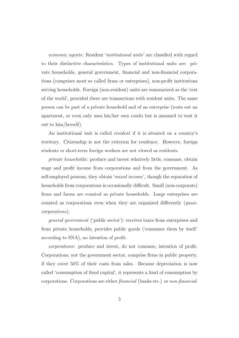
economic agents : Resident ‘institutional units ’ are classified with regard

to their distinctive characteristics. Types of institutional units are: pri-

vate households, general government, financial and non-financial corpora-

tions (comprises most so called firms or enterprises), non-profit institutions

serving households. Foreign (non-resident) units are summarized as the ‘rest

of the world’, provided there are transactions with resident units. The same

person can be part of a private household and of an enterprise (rents out an

apartment, or even only uses his/her own condo but is assumed to rent it

out to him/herself).

An institutional unit is called resident if it is situated on a country’s

territory. Citizenship is not the criterion for residence. However, foreign

students or short-term foreign workers are not viewed as residents.

private households : produce and invest relatively little, consume, obtain

wage and profit income from corporations and from the government. As

self-employed persons, they obtain ‘mixed income’, though the separation of

households from corporations is occasionally difficult. Small (non-corporate)

firms and farms are counted as private households. Large enterprises are

counted as corporations even when they are organized differently (quasi-

corporations).

general government (‘public sector’): receives taxes from enterprises and

from private households, provides public goods (‘consumes them by itself’

according to SNA), no intention of profit.

corporations : produce and invest, do not consume, intention of profit.

Corporations, not the government sector, comprise firms in public property,

if they cover 50% of their costs from sales. Because depreciation is now

called ‘consumption of fixed capital’, it represents a kind of consumption by

corporations. Corporations are either financial (banks etc.) or non-financial.

5

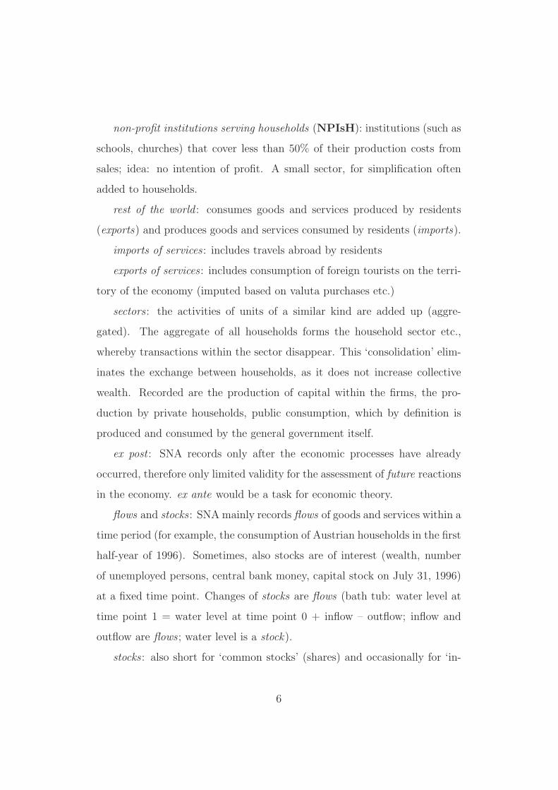
non-profit institutions serving households (NPIsH): institutions (such as

schools, churches) that cover less than 50% of their production costs from

sales; idea: no intention of profit. A small sector, for simplification often

added to households.

rest of the world : consumes goods and services produced by residents

(exports) and produces goods and services consumed by residents (imports).

imports of services: includes travels abroad by residents

exports of services: includes consumption of foreign tourists on the terri-

tory of the economy (imputed based on valuta purchases etc.)

sectors : the activities of units of a similar kind are added up (aggre-

gated). The aggregate of all households forms the household sector etc.,

whereby transactions within the sector disappear. This ‘consolidation’ elim-

inates the exchange between households, as it does not increase collective

wealth. Recorded are the production of capital within the firms, the pro-

duction by private households, public consumption, which by definition is

produced and consumed by the general government itself.

ex post : SNA records only after the economic processes have already

occurred, therefore only limited validity for the assessment of future reactions

in the economy. ex ante would be a task for economic theory.

flows and stocks : SNA mainly records flows of goods and services within a

time period (for example, the consumption of Austrian households in the first

half-year of 1996). Sometimes, also stocks are of interest (wealth, number

of unemployed persons, central bank money, capital stock on July 31, 1996)

at a fixed time point. Changes of stocks are flows (bath tub: water level at

time point 1 = water level at time point 0 + inflow – outflow; inflow and

outflow are flows ; water level is a stock).

stocks : also short for ‘common stocks’ (shares) and occasionally for ‘in-

6

ventories’ (beware of the possibility of confusion)

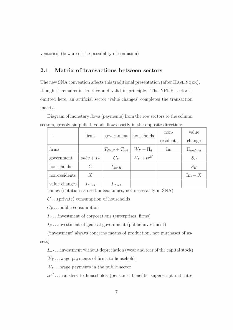
2.1 Matrix of transactions between sectors

The new SNA convention affects this traditional presentation (after Haslinger),

though it remains instructive and valid in principle. The NPIsH sector is

omitted here, an artificial sector ‘value changes’ completes the transaction

matrix.

Diagram of monetary flows (payments) from the row sectors to the column

sectors, grossly simplified, goods flows partly in the opposite direction:

→ firms government householdsnon-

residents

value

changes

firms Tdir,F + Tind WF + Πd Im Πund,net

government subv + IP CP WP + trH SP

households C Tdir,H SH

non-residents X Im − X

value changes IF,net IP,net

names (notation as used in economics, not necessarily in SNA):

C . . .(private) consumption of households

CP . . .public consumption

IF . . .investment of corporations (enterprises, firms)

IP . . .investment of general government (public investment)

(‘investment’ always concerns means of production, not purchases of as-

sets)

Inet . . .investment without depreciation (wear and tear of the capital stock)

WF . . .wage payments of firms to households

WP . . .wage payments in the public sector

trH . . .transfers to households (pensions, benefits, superscript indicates

7

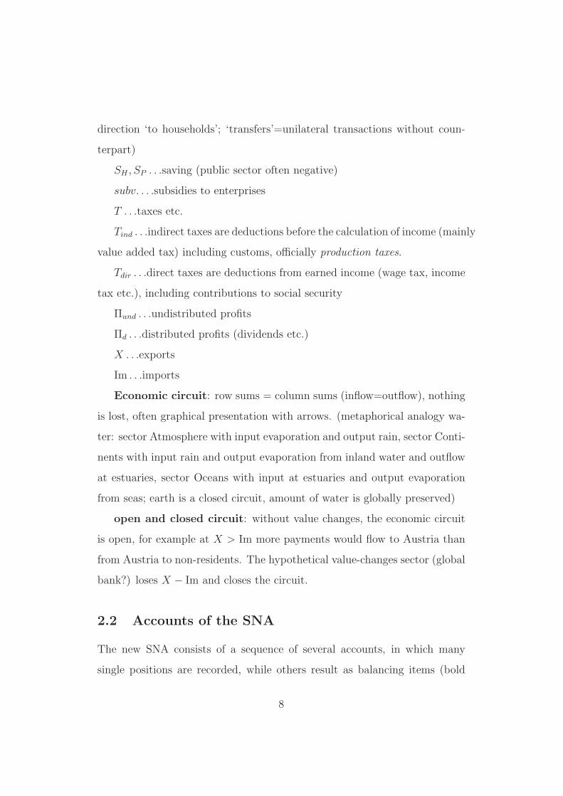
direction ‘to households’; ‘transfers’=unilateral transactions without coun-

terpart)

SH , SP . . .saving (public sector often negative)

subv. . . .subsidies to enterprises

T . . .taxes etc.

Tind . . .indirect taxes are deductions before the calculation of income (mainly

value added tax) including customs, officially production taxes.

Tdir . . .direct taxes are deductions from earned income (wage tax, income

tax etc.), including contributions to social security

Πund . . .undistributed profits

Πd . . .distributed profits (dividends etc.)

X . . .exports

Im . . .imports

Economic circuit: row sums = column sums (inflow=outflow), nothing

is lost, often graphical presentation with arrows. (metaphorical analogy wa-

ter: sector Atmosphere with input evaporation and output rain, sector Conti-

nents with input rain and output evaporation from inland water and outflow

at estuaries, sector Oceans with input at estuaries and output evaporation

from seas; earth is a closed circuit, amount of water is globally preserved)

open and closed circuit: without value changes, the economic circuit

is open, for example at X > Im more payments would flow to Austria than

from Austria to non-residents. The hypothetical value-changes sector (global

bank?) loses X − Im and closes the circuit.

2.2 Accounts of the SNA

The new SNA consists of a sequence of several accounts, in which many

single positions are recorded, while others result as balancing items (bold

8

type in the accounts). These accounts are calculated for all sectors (financial

and non-financial corporations, public households, private households and

NPIsH, rest of the world) and for the total economy.

2.2.1 Sectorial accounting

The accounts that are decomposed according to sectors (financial and non-

financial corporations, public households, private households and NPIsH) are

primarily income accounts, which focus on the contributions of individual

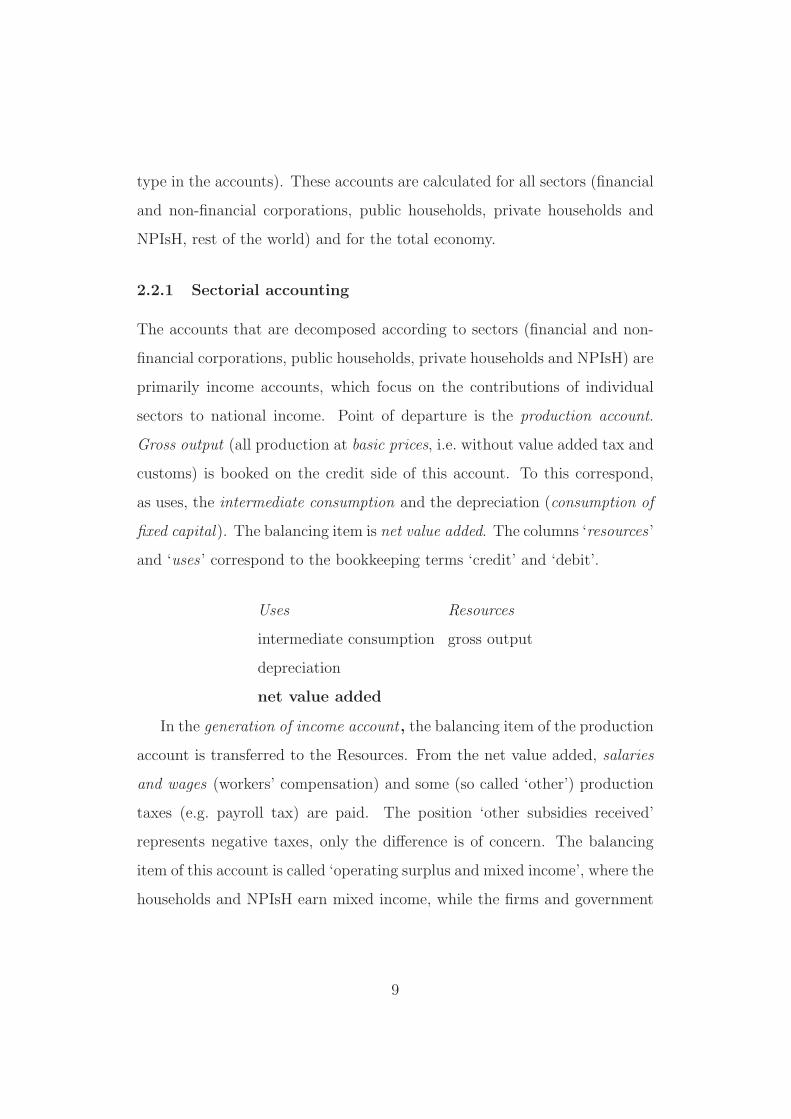
sectors to national income. Point of departure is the production account.

Gross output (all production at basic prices, i.e. without value added tax and

customs) is booked on the credit side of this account. To this correspond,

as uses, the intermediate consumption and the depreciation (consumption of

fixed capital). The balancing item is net value added. The columns ‘resources’

and ‘uses ’ correspond to the bookkeeping terms ‘credit’ and ‘debit’.

Uses Resources

intermediate consumption gross output

depreciation

net value added

In the generation of income account , the balancing item of the production

account is transferred to the Resources. From the net value added, salaries

and wages (workers’ compensation) and some (so called ‘other’) production

taxes (e.g. payroll tax) are paid. The position ‘other subsidies received’

represents negative taxes, only the difference is of concern. The balancing

item of this account is called ‘operating surplus and mixed income’, where the

households and NPIsH earn mixed income, while the firms and government

9

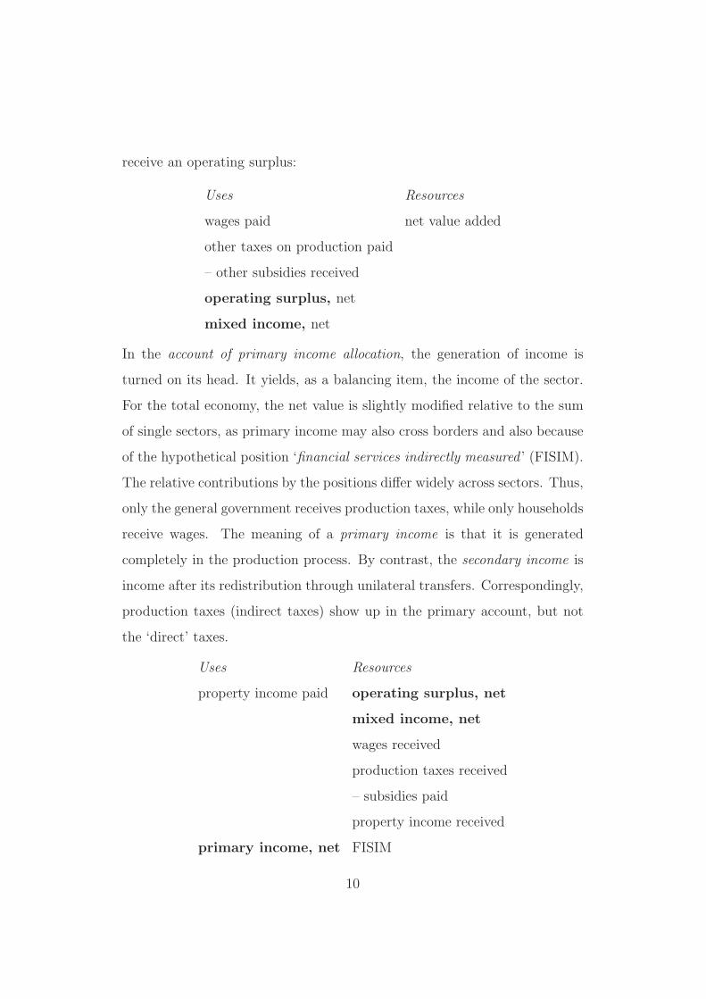
receive an operating surplus:

Uses Resources

wages paid net value added

other taxes on production paid

– other subsidies received

operating surplus, net

mixed income, net

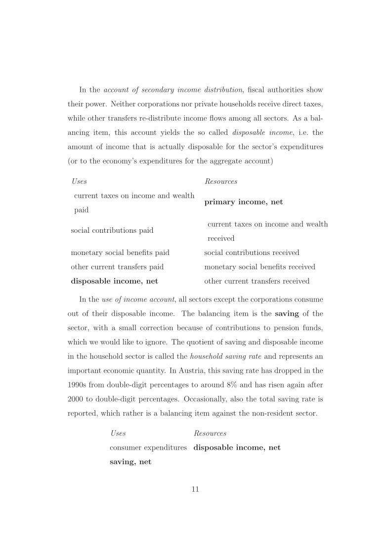
In the account of primary income allocation, the generation of income is

turned on its head. It yields, as a balancing item, the income of the sector.

For the total economy, the net value is slightly modified relative to the sum

of single sectors, as primary income may also cross borders and also because

of the hypothetical position ‘financial services indirectly measured ’ (FISIM).

The relative contributions by the positions differ widely across sectors. Thus,

only the general government receives production taxes, while only households

receive wages. The meaning of a primary income is that it is generated

completely in the production process. By contrast, the secondary income is

income after its redistribution through unilateral transfers. Correspondingly,

production taxes (indirect taxes) show up in the primary account, but not

the ‘direct’ taxes.

Uses Resources

property income paid operating surplus, net

mixed income, net

wages received

production taxes received

– subsidies paid

property income received

primary income, net FISIM

10

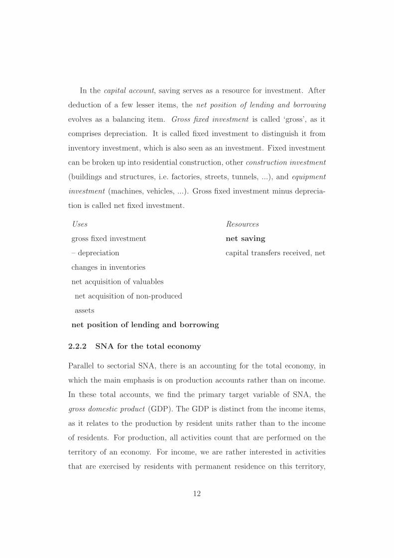
In the account of secondary income distribution, fiscal authorities show

their power. Neither corporations nor private households receive direct taxes,

while other transfers re-distribute income flows among all sectors. As a bal-

ancing item, this account yields the so called disposable income, i.e. the

amount of income that is actually disposable for the sector’s expenditures

(or to the economy’s expenditures for the aggregate account)

Uses Resources

current taxes on income and wealth

paidprimary income, net

social contributions paidcurrent taxes on income and wealth

received

monetary social benefits paid social contributions received

other current transfers paid monetary social benefits received

disposable income, net other current transfers received

In the use of income account, all sectors except the corporations consume

out of their disposable income. The balancing item is the saving of the

sector, with a small correction because of contributions to pension funds,

which we would like to ignore. The quotient of saving and disposable income

in the household sector is called the household saving rate and represents an

important economic quantity. In Austria, this saving rate has dropped in the

1990s from double-digit percentages to around 8% and has risen again after

2000 to double-digit percentages. Occasionally, also the total saving rate is

reported, which rather is a balancing item against the non-resident sector.

Uses Resources

consumer expenditures disposable income, net

saving, net

11

In the capital account, saving serves as a resource for investment. After

deduction of a few lesser items, the net position of lending and borrowing

evolves as a balancing item. Gross fixed investment is called ‘gross’, as it

comprises depreciation. It is called fixed investment to distinguish it from

inventory investment, which is also seen as an investment. Fixed investment

can be broken up into residential construction, other construction investment

(buildings and structures, i.e. factories, streets, tunnels, ...), and equipment

investment (machines, vehicles, ...). Gross fixed investment minus deprecia-

tion is called net fixed investment.

Uses Resources

gross fixed investment net saving

– depreciation capital transfers received, net

changes in inventories

net acquisition of valuables

net acquisition of non-produced

assets

net position of lending and borrowing

2.2.2 SNA for the total economy

Parallel to sectorial SNA, there is an accounting for the total economy, in

which the main emphasis is on production accounts rather than on income.

In these total accounts, we find the primary target variable of SNA, the

gross domestic product (GDP). The GDP is distinct from the income items,

as it relates to the production by resident units rather than to the income

of residents. For production, all activities count that are performed on the

territory of an economy. For income, we are rather interested in activities

that are exercised by residents with permanent residence on this territory,

12

whether these activities take place at home or abroad. For disposable income,

one is more interested in the persons who earn the income. For the GDP,

it is more important, where production occurs. Even for disposable income,

however, residents are not defined by their citizenship.

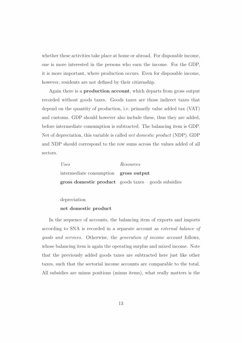
Again there is a production account, which departs from gross output

recorded without goods taxes. Goods taxes are those indirect taxes that

depend on the quantity of production, i.e. primarily value added tax (VAT)

and customs. GDP should however also include these, thus they are added,

before intermediate consumption is subtracted. The balancing item is GDP.

Net of depreciation, this variable is called net domestic product (NDP). GDP

and NDP should correspond to the row sums across the values added of all

sectors.

Uses Resources

intermediate consumption gross output

gross domestic product goods taxes – goods subsidies

depreciation

net domestic product

In the sequence of accounts, the balancing item of exports and imports

according to SNA is recorded in a separate account as external balance of

goods and services. Otherwise, the generation of income account follows,

whose balancing item is again the operating surplus and mixed income. Note

that the previously added goods taxes are subtracted here just like other

taxes, such that the sectorial income accounts are comparable to the total.

All subsidies are minus positions (minus items), what really matters is the

13

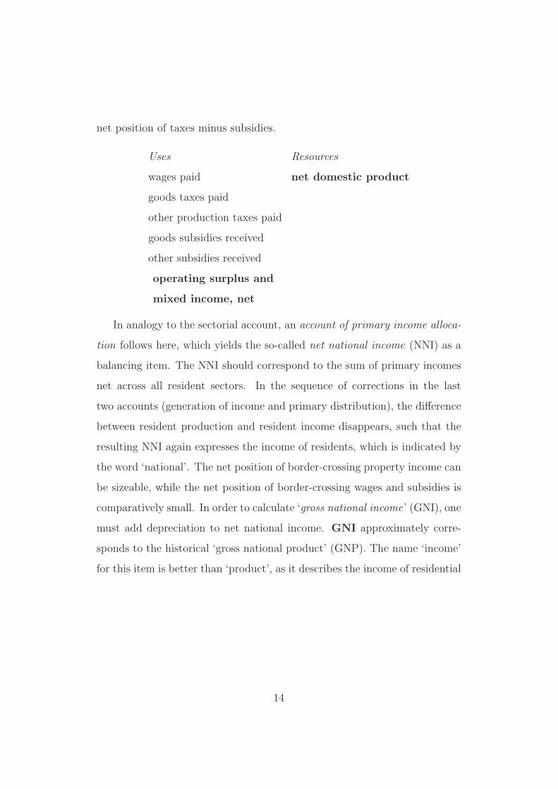
net position of taxes minus subsidies.

Uses Resources

wages paid net domestic product

goods taxes paid

other production taxes paid

goods subsidies received

other subsidies received

operating surplus and

mixed income, net

In analogy to the sectorial account, an account of primary income alloca-

tion follows here, which yields the so-called net national income (NNI) as a

balancing item. The NNI should correspond to the sum of primary incomes

net across all resident sectors. In the sequence of corrections in the last

two accounts (generation of income and primary distribution), the difference

between resident production and resident income disappears, such that the

resulting NNI again expresses the income of residents, which is indicated by

the word ‘national’. The net position of border-crossing property income can

be sizeable, while the net position of border-crossing wages and subsidies is

comparatively small. In order to calculate ‘gross national income’ (GNI), one

must add depreciation to net national income. GNI approximately corre-

sponds to the historical ‘gross national product’ (GNP). The name ‘income’

for this item is better than ‘product’, as it describes the income of residential

14

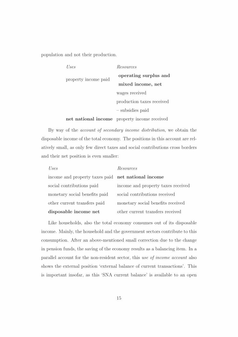
population and not their production.

Uses Resources

property income paidoperating surplus and

mixed income, net

wages received

production taxes received

– subsidies paid

net national income property income received

By way of the account of secondary income distribution, we obtain the

disposable income of the total economy. The positions in this account are rel-

atively small, as only few direct taxes and social contributions cross borders

and their net position is even smaller:

Uses Resources

income and property taxes paid net national income

social contributions paid income and property taxes received

monetary social benefits paid social contributions received

other current transfers paid monetary social benefits received

disposable income net other current transfers received

Like households, also the total economy consumes out of its disposable

income. Mainly, the household and the government sectors contribute to this

consumption. After an above-mentioned small correction due to the change

in pension funds, the saving of the economy results as a balancing item. In a

parallel account for the non-resident sector, this use of income account also

shows the external position ‘external balance of current transactions’. This

is important insofar, as this ‘SNA current balance’ is available to an open

15

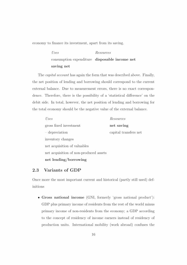
economy to finance its investment, apart from its saving.

Uses Resources

consumption expenditure disposable income net

saving net

The capital account has again the form that was described above. Finally,

the net position of lending and borrowing should correspond to the current

external balance. Due to measurement errors, there is no exact correspon-

dence. Therefore, there is the possibility of a ‘statistical difference’ on the

debit side. In total, however, the net position of lending and borrowing for

the total economy should be the negative value of the external balance.

Uses Resources

gross fixed investment net saving

– depreciation capital transfers net

inventory changes

net acquisition of valuables

net acquisition of non-produced assets

net lending/borrowing

2.3 Variants of GDP

Once more the most important current and historical (partly still used) def-

initions

• Gross national income (GNI, formerly ‘gross national product’):

GDP plus primary income of residents from the rest of the world minus

primary income of non-residents from the economy; a GDP according

to the concept of residency of income earners instead of residency of

production units. International mobility (work abroad) confuses the

16

concept (extreme examples Luxembourg, Kuwait). Persons with per-

manent residence in Austria are always counted as residents.

• Net domestic product: GDP minus depreciation.

• Net domestic product at factor costs: Net domestic product with-

out all production taxes (minus Tind plus subv).

• Net national income (formerly ‘net national product’): gross na-

tional income minus depreciation.

• Net disposable income of the economy: net national income (at

market prices, i.e. including all production taxes) plus balancing item

of border-crossing transfers.

• GDP (etc.) at basic prices: Intermediate stage between the calcula-

tion at market prices (i.e. including all production taxes) and the cal-

culation at producer prices (i.e. excluding all production taxes). Here,

only goods taxes (comprises as its most important parts the value added

tax and customs) minus goods subsidies are subtracted. Only after the

further subtraction of ‘other production taxes minus other subsidies’

(e.g., payroll tax), the value at producer prices is obtained. According

to convention, the original gross output is compiled at ‘basic prices ’,

GDP and NNI are then shown at market prices.

Factor costs: the compensation paid to the production factors capital

(machinery and buildings) and labor, by profits and wages, without taxes

(net minus subsidies).

Primary income: defined as income earned by direct participation in

the production process. Labor and property income. Formerly ‘factor in-

come’.

17

2.4 SNA=3 national accounts

In many countries, GDP was formerly calculated three times

• from production

• from its final uses

• from income

Particularly in the UK, three slightly different GDP variants were com-

puted. According to SNA convention today, the first of the three defines the

proper GDP. There is also a break-down according to different production

sectors (mining, agriculture, manufacturing etc.), which is not of central in-

terest in macroeconomics. An important component of this break-down is

industrial production, which is computed on a monthly basis and serves as a

fast business indicator.

Of fundamental interest in macroeconomics is the break-down of GDP

according to final uses

GDP = C + CP + I + X − Im , (1)

which is collected in a separate SNA account (Account 0). In economics,

GDP is denoted by the letter Y and government consumption by the letter

G. Note that, from the outlined sequence of accounts you obtain C from

the consumer expenditure of households (including NPIsH), Cp from the

consumer expenditures of general government, I from the capital account,

X − Im from the external account as an external balance. In order to obtain

an exact match of the left side (from production) and the right side (from

uses), one should observe:

18

• the changes in inventories (conceptually seen as investment: inventory

investment)

• the change in the stock of valuables (purchases of objects of art etc.)

and similar small positions

• a statistical difference (formerly often added to the smaller aggregates

as ‘inventory changes and statistical difference’)

Sometimes, private consumption C is broken down into:

• consumption of durable goods (cars, video recorders, ...)

• consumption of non-durable goods (clothing, food, books and journals,

...): proximity of purchase and utilization

• consumption of services (dining out, fitness studio, ...): not storable

Public consumption CP is broken down into:

• Collective consumption: indivisible utilization (e.g., street lighting)

• Individual consumption: can be allocated to individual persons (e.g.,

free education)

According to the concept of the new SNA, individual public consump-

tion and private consumption are summarized in the aggregate ‘individual

consumption’. The economic meaning of this convention is questionable.

Gross fixed investment I (‘gross’=includes depreciation, ‘fixed’=no

inventory investment; also comprises public investment; in SNA gross fixed

capital formation) is broken down into:

• investment in equipment (machinery, vehicles, ...)

19

• investment in construction (buildings and structures, includes residen-

tial construction)

The meaning of the distribution of income account for the determination

of disposable income etc. was already explained. In contrast to many other

parts of the SNA accounts, which exist in real terms (adjusted for inflation,

at constant prices, in the public sector difficult!) and also in nominal terms

(at current prices), the income distribution is calculated in nominal terms

only. An important derived quantity of the distribution accounts is the wage

quota, i.e. the share of compensation for labor in national income.

The disposable income of households YD serves as the basis for the cal-

culation of the household saving rate

qSH =YD − C

YD

.

In Austria, this quotient currently is around 13%.

2.5 External balances

The balance of payments registers all transactions of goods, services, pay-

ments across borders. Because of different concepts, it does not match the

SNA balances exactly:

1. goods balance (only goods, in Austria approximately neutral net posi-

tion)

2. services balance (primarily tourism, in Austria positive net position,

and also other services)

3. external balance of primary income (compensation of border workers,

primarily border-crossing property income, in Austria passive)

20

4. external balance of transfers (transactions without counterpart, in Aus-

tria passive)

Positions 1–2 together are the so-called ‘trade balance’, Position 1–4 yield

the current accounts balance. The current accounts balance should match,

with inverted sign, the balance of capital flows (capital accounts balance,

short- and long-run capital flows; note the usage of the word ‘capital’ that

does not denote produced means of production here). A difference of the

two positions may stem from the change in reserves of currency and gold

in the central bank, and from diverse statistical discrepancies. All balances

together are called the balance of payments. Therefore, there cannot be a

deficit in the balance of payments, while there may be a current account

deficit.

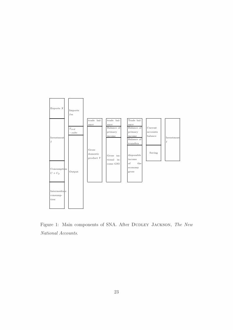
Figure 1 summarizes the SNA and also includes all external balances. The

first two bars represent the gross sum of production accounting. Exports, in-

vestment, public and private consumption contribute as well as intermediate

consumption (expenditure accounting). This gross sum must correspond to

imports plus output (production accounting). Because output is evaluated

without goods taxes, everything else at market prices, goods taxes (minus

subsidies) must be added to the production side.

The third bar yields GDP as the difference of output (plus product taxes)

minus intermediate consumption. Exports minus imports yield the trade

balance (here, in the example, passive). The entire bar represents all products

available to the economy.

The fourth bar calculates GNI as the sum of GDP and the balance of pri-

mary income (here passive). A part of domestic production benefits foreign

income earners.

21

The fifth bar calculates the disposable income of the economy as the sum

of GNI and the balance of secondary income (here passive), i.e. the balance of

transfers. A part of domestic income is transmitted to the rest of the world.

The sixth bar collects the three partial balances in the current accounts

balance. Disposable income minus consumption yields the saving of the

economy.

The seventh bar represents investment. To finance investment, the econ-

omy can use domestic saving and also the negative balance of the current

accounts. In this diagram, the part of investment financed by the foreign

deficit, i.e. by debt, is large. This negative balance of the current accounts

is also called saving of the rest of the world. The larger the deficit, the more

can be invested.

2.6 Other statistics related to SNA

Wealth is a stock variable and notoriously difficult to compile (human cap-

ital, unknown value of assets etc.). Household wealth can be estimated from

consumer expenditures on durables and assumptions about the depreciation

of these durable goods. Data on monetary wealth is provided by banks

(checking accounts, saving accounts, bonds, shares). The capital stock

(stock of produced means of production) results from depreciation rates for

types of capital goods and from gross fixed investment. The stock of in-

ventories results from inventory changes etc.

Input-output (IO) tables are large matrix tables that report the flows

of goods and services among subsectors of an economy, admit detailed in-

formation about intermediary consumption, which is necessary for final pro-

duction in a certain sub-sector.

Price indexes (deflators) must be calculated for the GDP and for all of

22

Exports X

Investment

I

Consumption

C + Cp

Intermediate

consump-

tion

Output

Tind

−subv

Imports

Im

Gross

domestic

product Y

trade bal-

ance

Gross na-

tional in-

come GNI

Balance of

primary

income

trade bal-

ance

disposable

income

of the

economy

gross

Balance of

transfers

Balance of

primary

income

Trade bal-

ance

Saving

Current

accounts

balanceInvestment

I

Figure 1: Main components of SNA. After Dudley Jackson, The New

National Accounts.

23

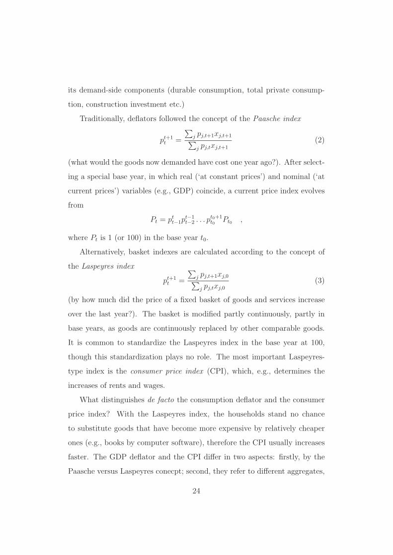
its demand-side components (durable consumption, total private consump-

tion, construction investment etc.)

Traditionally, deflators followed the concept of the Paasche index

pt+1

t =

∑j pj,t+1xj,t+1

∑j pj,txj,t+1

(2)

(what would the goods now demanded have cost one year ago?). After select-

ing a special base year, in which real (‘at constant prices’) and nominal (‘at

current prices’) variables (e.g., GDP) coincide, a current price index evolves

from

Pt = ptt−1p

t−1

t−2 . . . pt0+1

t0Pt0 ,

where Pt is 1 (or 100) in the base year t0.

Alternatively, basket indexes are calculated according to the concept of

the Laspeyres index

pt+1

t =

∑j pj,t+1xj,0

∑j pj,txj,0

(3)

(by how much did the price of a fixed basket of goods and services increase

over the last year?). The basket is modified partly continuously, partly in

base years, as goods are continuously replaced by other comparable goods.

It is common to standardize the Laspeyres index in the base year at 100,

though this standardization plays no role. The most important Laspeyres-

type index is the consumer price index (CPI), which, e.g., determines the

increases of rents and wages.

What distinguishes de facto the consumption deflator and the consumer

price index? With the Laspeyres index, the households stand no chance

to substitute goods that have become more expensive by relatively cheaper

ones (e.g., books by computer software), therefore the CPI usually increases

faster. The GDP deflator and the CPI differ in two aspects: firstly, by the

Paasche versus Laspeyres conecpt; second, they refer to different aggregates,

24

private consumption and gross domestic product, the latter one including

investment goods not consumed by households.

hedonic prices: technical products (cars, computers) develop fast. Some

experts argue that these should not be valued at the market price, but at the

price of their inner characteristics (fuel consumption, speed of calculation).

This concept often yields a general decrease in the price of such goods by

increase in quality, though the problem remains whether the customers are

forced to consume an additional and relatively cheap ‘quality’ of such goods

(tinted car windows, automatically installed software). The concept is partly

used by statistical agencies for the calculation of all indexes.

Chaining: since 2004, SNA has replaced the original Paasche indexes by

chain indexes, weighting quantities at successive time points geometrically. A

consequence is that identities—such as the important Account 0 identity—do

not hold exactly for real quantities any more.

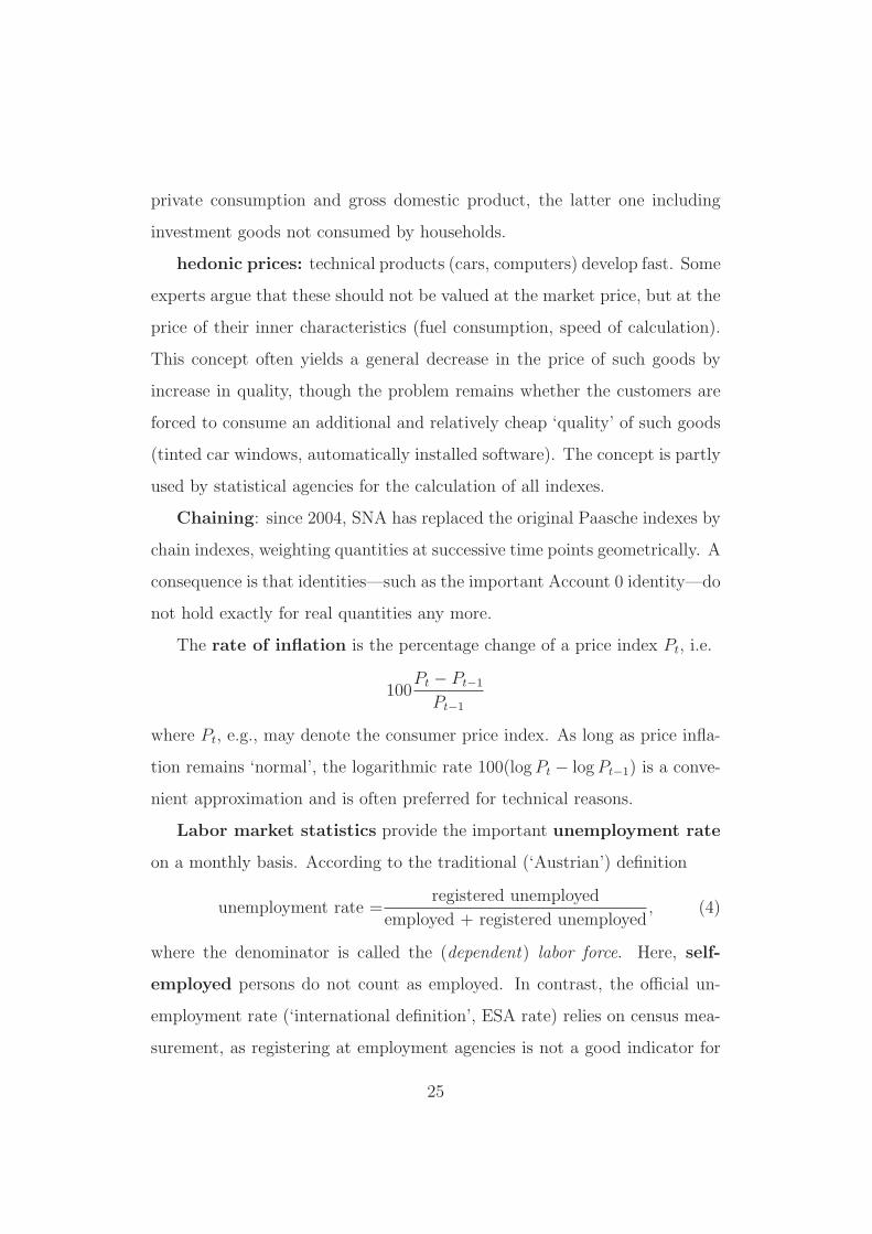
The rate of inflation is the percentage change of a price index Pt, i.e.

100Pt − Pt−1

Pt−1

where Pt, e.g., may denote the consumer price index. As long as price infla-

tion remains ‘normal’, the logarithmic rate 100(log Pt − log Pt−1) is a conve-

nient approximation and is often preferred for technical reasons.

Labor market statistics provide the important unemployment rate

on a monthly basis. According to the traditional (‘Austrian’) definition

unemployment rate =registered unemployed

employed + registered unemployed, (4)

where the denominator is called the (dependent) labor force. Here, self-

employed persons do not count as employed. In contrast, the official un-

employment rate (‘international definition’, ESA rate) relies on census mea-

surement, as registering at employment agencies is not a good indicator for

25

unemployment (no registration, when there is no chance of obtaining benefits

or if search is hopeless; fake registration of persons working in the shadow

economy) in many countries. According to this convention, self-employed

persons are included. In Austria, the ‘international’ concept leads to a lower

rate; in Spain, it leads to a higher rate.

2.7 Critique of National Accounts

1. SNA measures incorrectly

(a) Measurement and numbers are bad: Critique of reducing the real

world to data (atypical for a quantitative science, such as eco-

nomics)

(b) SNA does not measure welfare ⇒ social indicators, questionnaires

etc. (borderline to sociology)

(c) SNA measures flows, whereas true wealth is expressed by stocks

of property and possessions.

2. SNA measures too much

(a) regrettable necessities should not be measured, such as road acci-

dents, criminal activity, expenditures for longer commute to work,

as these do not increase welfare: definition of boundaries is diffi-

cult, strong consequences for international and intertemporal com-

parisons unlikely (military goods even now only contribute, if they

can also be used for civilian purposes)

(b) damage to health and the environment should be subtracted. Throw-

away goods should not increase wealth ⇒ slower growth if such

26

concepts are considered tentatively (Nordhaus/Tobin: measure

of economic welfare MEW instead of GDP)

3. SNA measures too little

(a) economic activities, which do not touch official markets (house-

hold work, so-called shadow economy), are not compiled accu-

rately (household work is deliberately excluded, as: (1) it is dif-

ficult to measure, (2) externalizing of services in principle even

now an indicator of welfare, (3) household services as component

of GDP would destroy the differentiation between unemployment

and employment; shadow economy is included in official GDP, al-

though its assessment is concededly difficult; illegal production is

by definition a part of GDP!)

(b) quality of life, leisure, creation of national parks, cleaning of air

and water are not valued sufficiently, as these are not market goods

and do not have market prices (task for environmental economics)

27

3 The goods market

Wherever necessary, it is assumed that households and firms are identical

and produce and consume only one good. This good serves as a consump-

tion good as well as an investment good. Demand is assumed to be satisfied

immediately by supply at a given and fixed price. The decomposition (Ac-

count 0) of national income Y (or GDP, these are assumed as equal in what

follows) according to uses

Y = C + I + G + X − Im (5)

(consumption C, investment I, government expenditure G loosely corre-

sponds to the CP from SNA, exports X, imports Im) simplifies to

Y = C + I + G (6)

in a closed economy, which does not communicate with the rest of the

world by means of imports or exports (as opposed to an open economy). At

first, it will be assumed that the economy is closed.

Consumption C: households consume out of their disposable income,

we write

C = C(YD)

+

This is a (for the moment, not exactly specified) consumption function.

The sign ‘+’ indicates that consumption rises with increasing income and

falls with decreasing income, i.e. it reacts ‘positively’. A simple functional

form is the linear specification

C = c0 + c1YD (7)

28

with c1 > 0 and typically also c0 > 0. This so-called Keynes consumption

function contains two parameters c0, c1, i.e. not directly observable, fixed

constants. As a behavioral equation, it describes the action of households

as depending on their income. By contrast, the simplifying relation

YD = Y − T (8)

with taxes T is not a behavioral equation, but rather a definitional equa-

tion (identity). In more detail, the variable T may be identified with ‘in-

come taxes minus transfers from government to households’ and may even

be thought to comprise social contributions and benefits.

‘Lump sum’: except for some exercise examples, taxes T are assumed

to be independent of income. Each identical household pays a fixed amount

to the government, a ‘lump sum’.

The parameter c0 is the autonomous consumption of the economy.

Because the households are all alike, c0 is the sum of all expenditures of all

households that is necessary for their survival, if these do not receive any

income.

The parameter c1 is the marginal propensity to consume and de-

scribes, by how much consumption rises, if households receive an increase in

their income by, e.g., one euro. In this case, they increase consumption by

c1 euro. It makes sense to require c1 < 1, i.e. c1 ∈ (0, 1). One also writes

c1 =∂C

∂YD

(9)

Unlike c1, the average propensity to consume

C

YD

=c0

YD

+ c1 (10)

is not a constant, but falls with increasing income. C/YD answers the ques-

tion, how much out of the total income is consumed, not out of a ‘marginal’

29

additional income. Falling average, but constant marginal propensity to con-

sume was one of the famous Keynes axioms.

Investment I, government expenditure G, taxes T : are kept fixed

and are, as ‘exogenous’ variables, not determined in the model; no relation-

ship between G and T ; exogenous (determined outside the model) variables

act like parameters, though, unlike those, they are observed directly. For-

mally, one writes:

I = I (11)

G = G (12)

T = T (13)

The behavioral equation (7), the definitional equation (8), and the three iden-

tities that express exogeneity (11), (12), (13) describe the aggregate demand

in the simple closed economy.

The supply results from the quantity of the produced good Y .

Equilibrium on the goods market, i.e. a cleared goods market, in which

there are no increasing inventories and no unsatisfied and hungry consumers,

means that Y and aggregate demand Z = C + I + G are equal, i.e. Y = Z,

or

Y = c0 + c1YD + I + G

= c0 + c1(Y − T ) + I + G

and thus

Y =1

1 − c1

(c0 + I + G − c1T )

Thought experiments

1. We increase government expenditure G by 1 euro. This increases na-

tional income Y by 1/(1 − c1) euro. Because c1 ∈ (0, 1), for example

30

c1 = 0.9, Y increases by more than one euro, for example by 10 euro.

2. We increase investment I by 1 euro. Again Y increases by 1/(1 − c1)

euro, in the numerical example by 10 euro.

3. We increase autonomous consumption c0, for example by a campaign

of optimism. Again, Y increases by 1/(1 − c1) euro.

4. We increase taxes by 1 Euro. Now Y falls by c1/(1 − c1) euro.

The important value 1/(1 − c1) is called the (fiscal) multiplier, as it

multiplies the increase of an exogenous input in the aggregate output. This

multiplier effect is caused by the following mechanism: additional consumer

demand leads to an increase in total aggregate demand Z, which is satisfied

by the firms immediately, whereby Y increases once more, as income equals

production, etc.

Saving propensity and multiplier: If YD−C is interpreted as house-

hold saving SH , then 1− c1 is the (marginal) saving propensity of house-

holds, if c1 is a propensity to consume, as

SH = YD − C = YD − (c0 + c1YD) = −c0 + (1 − c1)YD

The bigger the saving propensity, i.e. the smaller the propensity to consume,

the smaller is the multiplier, and vice versa. At a saving propensity of 1,

the multiplier becomes 1, i.e. it does not multiply anything. At a saving

propensity of 0, the multiplier becomes ∞. This would be nonsense and

must be ruled out.

Empirical evidence (Figure 2): in line with the theoretical concept,

the propensity to consume appears to be slightly less than 1. A statisti-

cal regression estimation yields a value of c1 = 0.89 and c0 = −13. The

propensity to consume is reasonable (on average, households save 11% of

31

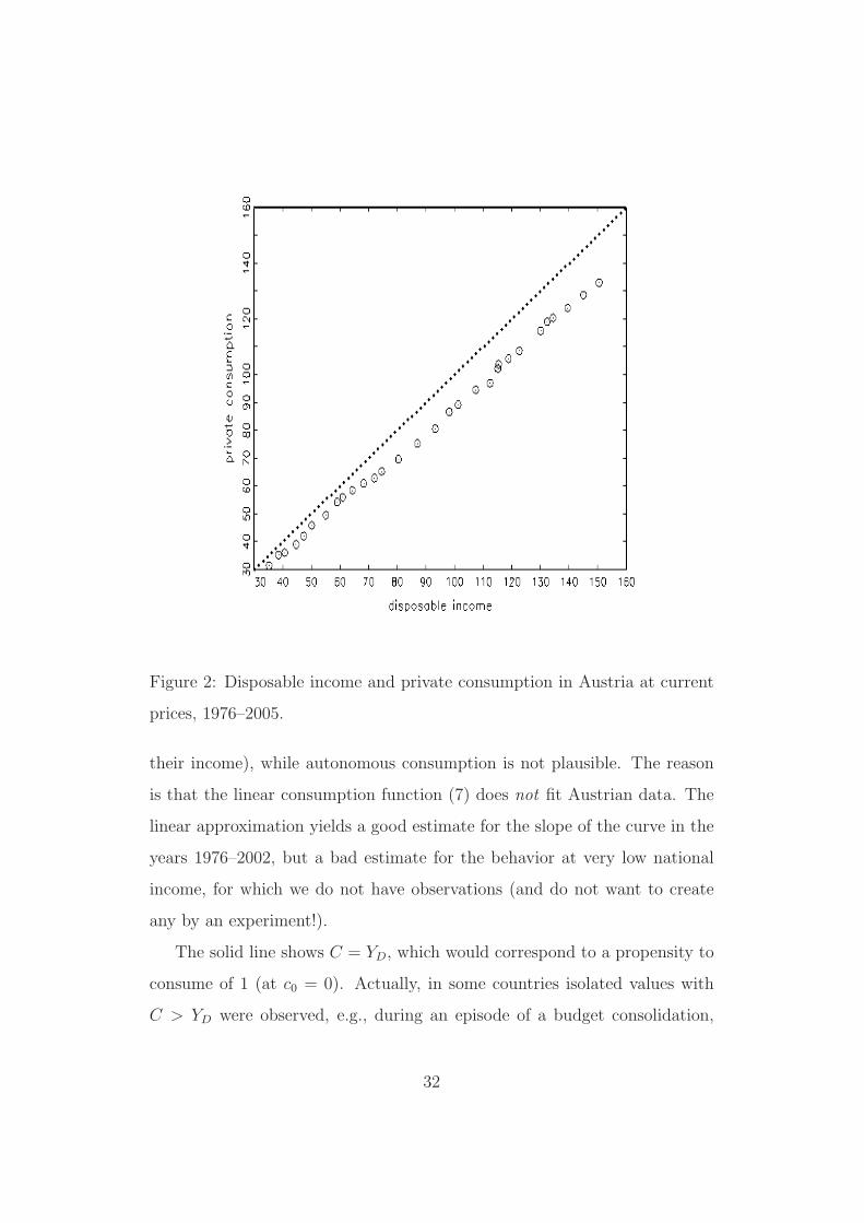
Figure 2: Disposable income and private consumption in Austria at current

prices, 1976–2005.

their income), while autonomous consumption is not plausible. The reason

is that the linear consumption function (7) does not fit Austrian data. The

linear approximation yields a good estimate for the slope of the curve in the

years 1976–2002, but a bad estimate for the behavior at very low national

income, for which we do not have observations (and do not want to create

any by an experiment!).

The solid line shows C = YD, which would correspond to a propensity to

consume of 1 (at c0 = 0). Actually, in some countries isolated values with

C > YD were observed, e.g., during an episode of a budget consolidation,

32

though not in Austria.

Saving is investment (the IS identity). The saving of households (a

flow, not ‘savings’, this could be the stock of saving accounts!) is that part

of income that is not consumed

SH = YD − C = Y − T − C (14)

Noting that Y = C + I + G we obtain

SH = I + G − T. (15)

If government runs a balanced budget, then its expenditure G equals taxes

T , G = T . This implies SH = I, “saving equals investment”. If government

runs a budget surplus (at the expense of the rest of the economy), then T > G

and therefore I > SH . If government consumes more than its revenues (a

budget deficit), then T < G and therefore I < SH . If one views T − G as

‘government saving’ SP , then

SH + SP = I (16)

Thus, investment equals saving of households plus government saving. Typ-

ically, SP will be negative.

Where is the saving of firms? The saving of enterprises corresponds

to undistributed profits. In this simple model, it is assumed that (8) holds,

households receive the total income minus taxes. In this model, the saving

of firms is therefore 0.

Is saving good or bad? (Schoolchildren often learn that saving is

a good thing) In the short run, saving has a contractionary effect, i.e., a

negative effect on output. Lower c0 decreases aggregate income by c0/(1−c1).

Lower c1 has an even stronger negative effect. Because a contractionary effect

of saving appears to be a ‘paradox’, this is sometimes called the saving

33

paradox (paradox of thrift, first implication). It can also be shown that,

in the model, a decrease of c0 or c1 implies such a strong decrease in Y

that SH (which depends on Y ) does not change at all (Exercise, paradox of

thrift, second implication). In the long run, the saving paradox disappears,

as saving increases the growth potential of the economy, causes the interest

rate to fall, and increases investment. These mechanisms are absent in the

simple model with I = I. (16) is only an identity and does not describe

economic behavior.

Is it preferable to increase government expenditure or to de-

crease taxes? In the model, a 1 billion euro increase in G at c1 = 0.9 yields

an additional income of 10 billion euro, while a decrease of T by the same

amount only yields 9 billion euro. G directly affects aggregate income, while

T only affects the disposable income and household consumption, whereby

saving annihilates a part 1 − c1.

4 Financial markets

Many possibilities are available to a household who has to allocate its income.

The largest part of the disposable income is consumed, the remainder (7–

12%) is ‘saved’. For saving, the following ‘assets’ can be used:

1. cash money (currency): originally promissory notes on the central

bank. Universally accepted for transactions, but bears no interest.

Liquidity is maximal, interest rate is 0.

2. checking accounts (demand deposits): short-run assets at banks.

Increasingly used for transactions (Quick Cash, Debit Card), very low

interest. Liquidity is high, interest rate nearly 0. Included even in

narrow-sense money (M1).

34

3. saving accounts (and time deposits): longer-run assets at banks.

Must be exchanged for money to enable transactions (limited liquidity),

but bear interest. Fast exchange for cash with small and standardized

transaction costs, therefore included in wide-sense money (M3).

4. bonds (risk-free securities with fixed interest): promissory notes at

good debtors, can be purchased at banks (brokers). Better interest,

must be sold for transactions.

5. shares: certificates of shared ownership at corporations. Uncertain,

though often good interest (return, dividends). Usually purchased via

banks (brokers) at a stock exchange and sold at variable prices.

6. real estate, stamps, antiques: uncertain interest, low liquidity (sta-

tistically, partly consumption!).

The aggregate stock of these assets is the wealth of households. Note that

household wealth does not contain the stock of consumer durables (cars and

dishwashers) with their negative rate of interest due to depreciation. Wealth

and its components are stocks, which increase by adding the flow variable

‘income’ and diminish by subtracting the flow variable ‘consumption’.

Assumption: in the closed economy there are only money and bonds.

The problem of households consists in distributing their wealth optimally

among money (M) and bonds (B), i.e. to find M and B such that M +

B = $W . The symbol ‘$W ’ indicates that wealth and its components are

measured at current prices (in nominal terms).

4.1 Demand for money and bonds

Demand for money (Md for money demand). Money serves for trans-

actions, whose amount is proportional to national income ($Y for nominal

35

national income). High income means many transactions. When interest i

on bonds is high, households do not want to forego the additional income

out of interest and keep little money. One writes

Md = Md($Y, i)

+ −

or, more specifically and simpler

Md = $Y · L(i)

with the function L(i), which falls in its argument i. The letter L is for

‘liquidity’. At an interest rate of 0, i = 0, all wealth is kept as money. At a

high interest rate, relatively little money is kept. Thus, one has i ≥ 0 and

L(i) > 0.

For fixed income $Y , one sees a falling function (Fig. 3), which is drawn

with i on its y axis (ordinate axis) and with M on its x axis (abscissa axis),

for technical reasons. The higher $Y , the more do the curves move to their

right. At every interest rate i, more money is demanded.

Demand for bonds Bd. This results from the budget constraint and

from money demand as

Bd = $W − Md

= $W − $Y L(i)

Larger wealth causes an increased demand for bonds, higher interest also

raises the demand for bonds. Higher income increases the stock of wealth

but also decreases money demand. In the short run, we assume that $W is

exogenous, therefore an increase in income will cause a fall in the demand

for bonds.

36

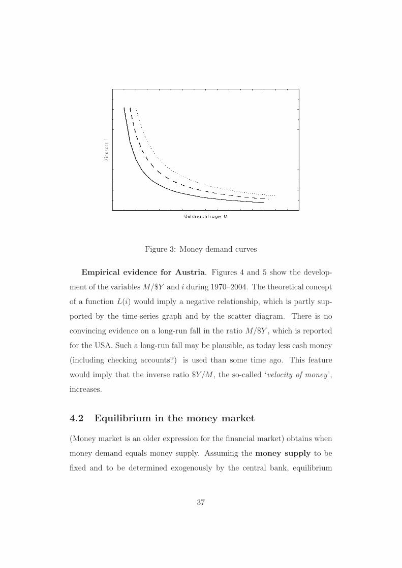
Figure 3: Money demand curves

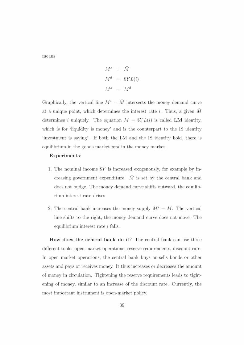
Empirical evidence for Austria. Figures 4 and 5 show the develop-

ment of the variables M/$Y and i during 1970–2004. The theoretical concept

of a function L(i) would imply a negative relationship, which is partly sup-

ported by the time-series graph and by the scatter diagram. There is no

convincing evidence on a long-run fall in the ratio M/$Y , which is reported

for the USA. Such a long-run fall may be plausible, as today less cash money

(including checking accounts?) is used than some time ago. This feature

would imply that the inverse ratio $Y/M , the so-called ‘velocity of money ’,

increases.

4.2 Equilibrium in the money market

(Money market is an older expression for the financial market) obtains when

money demand equals money supply. Assuming the money supply to be

fixed and to be determined exogenously by the central bank, equilibrium

37

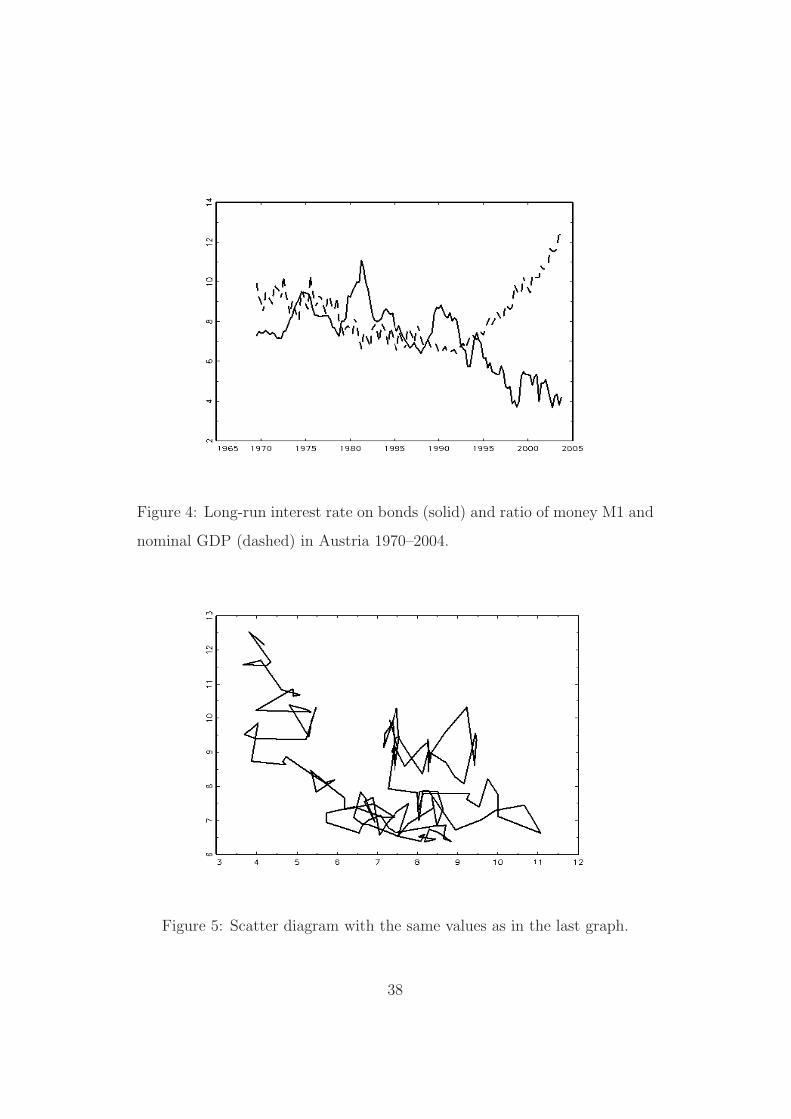
Figure 4: Long-run interest rate on bonds (solid) and ratio of money M1 and

nominal GDP (dashed) in Austria 1970–2004.

Figure 5: Scatter diagram with the same values as in the last graph.

38

means

M s = M

Md = $Y L(i)

M s = Md

Graphically, the vertical line M s = M intersects the money demand curve

at a unique point, which determines the interest rate i. Thus, a given M

determines i uniquely. The equation M = $Y L(i) is called LM identity,

which is for ‘liquidity is money’ and is the counterpart to the IS identity

‘investment is saving’. If both the LM and the IS identity hold, there is

equilibrium in the goods market and in the money market.

Experiments:

1. The nominal income $Y is increased exogenously, for example by in-

creasing government expenditure. M is set by the central bank and

does not budge. The money demand curve shifts outward, the equilib-

rium interest rate i rises.

2. The central bank increases the money supply M s = M . The vertical

line shifts to the right, the money demand curve does not move. The

equilibrium interest rate i falls.

How does the central bank do it? The central bank can use three

different tools: open-market operations, reserve requirements, discount rate.

In open market operations, the central bank buys or sells bonds or other

assets and pays or receives money. It thus increases or decreases the amount

of money in circulation. Tightening the reserve requirements leads to tight-

ening of money, similar to an increase of the discount rate. Currently, the

most important instrument is open-market policy.

39

Reserve requirements. Obligatory reserves of banks that are held

at the central bank. Formerly, the central bank paid no interest on such

monetary reserves. The original intention was to guarantee the banks’ savings

accounts, today reserve requirements are just means of controlling the money

supply. Today, reserves have become interest-bearing (∼ 2%). Thus, this

interest rate be used as another instrument of controlling the money supply.

Discount rate. An interest rate for transactions between the central

bank and banks. A higher discount rate does not automatically imply a

higher interest rate in the money market, though some positive influence is

reasonable to assume.

4.3 Price of bonds and interest rate

In real-world financial markets, the interest rate of a bond is not determined

directly, but indirectly via the bond price. Assume that a bond is in circula-

tion at time point t, while its owner receives at maturity t+1 a value of 100.

That is, assume that ‘100’ and the maturity date are printed on the bond.

Then, the price of the bond in t, PBt, determines the interest because of

it =100 − PBt

PBt

,

i.e. not in percentage points, e.g., it = 0.07. Conversely, if i is given, the

bond price can be calculated as

PB =100

1 + i.

Because i > 0, it must hold that PB < 100 .

40

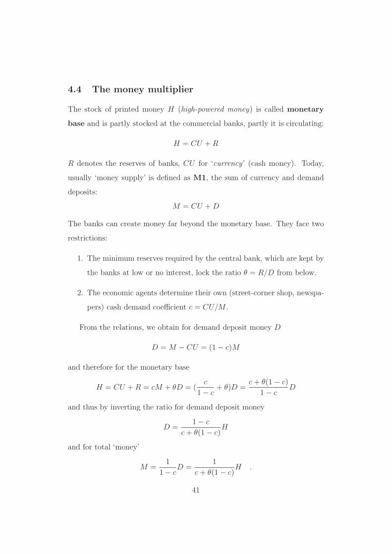
4.4 The money multiplier

The stock of printed money H (high-powered money) is called monetary

base and is partly stocked at the commercial banks, partly it is circulating:

H = CU + R

R denotes the reserves of banks, CU for ‘currency ’ (cash money). Today,

usually ‘money supply’ is defined as M1, the sum of currency and demand

deposits:

M = CU + D

The banks can create money far beyond the monetary base. They face two

restrictions:

1. The minimum reserves required by the central bank, which are kept by

the banks at low or no interest, lock the ratio θ = R/D from below.

2. The economic agents determine their own (street-corner shop, newspa-

pers) cash demand coefficient c = CU/M .

From the relations, we obtain for demand deposit money D

D = M − CU = (1 − c)M

and therefore for the monetary base

H = CU + R = cM + θD = (c

1 − c+ θ)D =

c + θ(1 − c)

1 − cD

and thus by inverting the ratio for demand deposit money

D =1 − c

c + θ(1 − c)H

and for total ‘money’

M =1

1 − cD =

1

c + θ(1 − c)H .

41

The value 1/{c + θ(1 − c)} is called the money multiplier, as it indicates,

by how much the money supply increases, if the central bank prints one

additional unit of cash money. For small c and small θ, the multiplier becomes

particularly large.

Example. Blanchard assumes θ = 0.1, we further assume that c =

0.05 (compare this to your own private allocation between cash and demand

deposits!). Then, the purchase of a bond for 1000 euro by the central bank

against emission of ten 100 euro notes causes the bond seller to increase his

demand deposit by 950 euro, while 50 euro of cash remain in the trouser

pocket. The bank keeps 95 euro as reserve and buys bonds for 855 euro from

a different bond seller. This bond seller keeps 42.75 euro in cash in the pocket

of her jacket, while she increases her demand deposit by 855-42.75=812. 25

euro. Even now, money M1 has almost doubled, but the chain continues and

finally leads to 1/(0.05+0.1*0.95) euro, i.e. around 7000 euro, therefore to a

sevenfold increase according to the above formula.

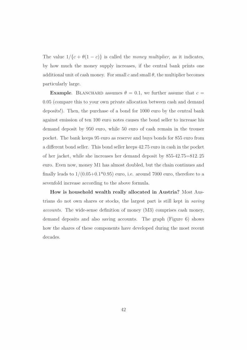
How is household wealth really allocated in Austria? Most Aus-

trians do not own shares or stocks, the largest part is still kept in saving

accounts. The wide-sense definition of money (M3) comprises cash money,

demand deposits and also saving accounts. The graph (Figure 6) shows

how the shares of these components have developed during the most recent

decades.

42

Figure 6: Development of monetary wealth components for the years 1962–

2004 in Austria.

43

5 The IS-LM model

If one looks at the goods and financial markets jointly, then both the equilib-

rium condition on the goods market (IS) and on the financial market (LM)

should hold. In the tradition of Keynes and Hicks, the emphasis is on the

behavior of income Y and of the interest rate i. For this purpose, the model

needs a reaction to interest rates on the goods market. Such a reaction is

most likely in investment behavior.

5.1 Investment function

The simple assumption I = I is now replaced by a useful investment function.

Investors react to two important variables:

1. expected sales should affect investment plans. These are not known,

though observed output Y should be a good indicator for expected

sales.

2. the interest rate determines the costs of loans that are required to

execute investment plans.

It follows that one may depart from an investment function such as

I = I(Y, i)

(+,−)

A functional form will, however, not be specified.

Empirical evidence. A systematic negative reaction of gross fixed in-

vestment to interest rates is difficult to establish empirically. The graphs

show scatter diagrams of the investment ratio I/Y and of its real growth

rate against a (nominal) interest rate and only vaguely indicate a negative

44

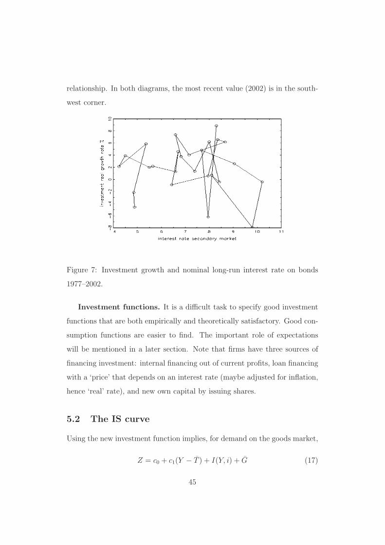
relationship. In both diagrams, the most recent value (2002) is in the south-

west corner.

Figure 7: Investment growth and nominal long-run interest rate on bonds

1977–2002.

Investment functions. It is a difficult task to specify good investment

functions that are both empirically and theoretically satisfactory. Good con-

sumption functions are easier to find. The important role of expectations

will be mentioned in a later section. Note that firms have three sources of

financing investment: internal financing out of current profits, loan financing

with a ‘price’ that depends on an interest rate (maybe adjusted for inflation,

hence ‘real’ rate), and new own capital by issuing shares.

5.2 The IS curve

Using the new investment function implies, for demand on the goods market,

Z = c0 + c1(Y − T ) + I(Y, i) + G (17)

45

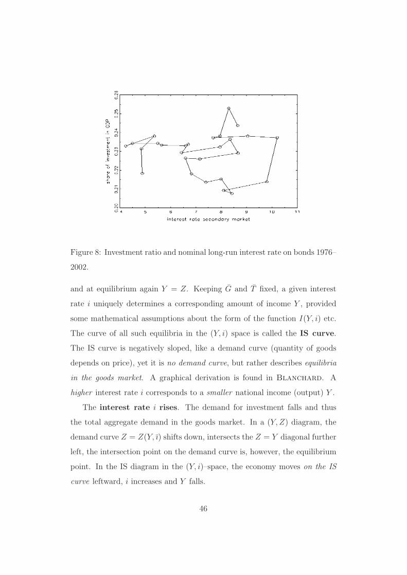
Figure 8: Investment ratio and nominal long-run interest rate on bonds 1976–

2002.

and at equilibrium again Y = Z. Keeping G and T fixed, a given interest

rate i uniquely determines a corresponding amount of income Y , provided

some mathematical assumptions about the form of the function I(Y, i) etc.

The curve of all such equilibria in the (Y, i) space is called the IS curve.

The IS curve is negatively sloped, like a demand curve (quantity of goods

depends on price), yet it is no demand curve, but rather describes equilibria

in the goods market. A graphical derivation is found in Blanchard. A

higher interest rate i corresponds to a smaller national income (output) Y .

The interest rate i rises. The demand for investment falls and thus

the total aggregate demand in the goods market. In a (Y, Z) diagram, the

demand curve Z = Z(Y, ı) shifts down, intersects the Z = Y diagonal further

left, the intersection point on the demand curve is, however, the equilibrium

point. In the IS diagram in the (Y, i)–space, the economy moves on the IS

curve leftward, i increases and Y falls.

46

The interest rate i falls. The economy moves on the IS curve to the

right, i falls, while Y increases.

Taxes T are increased. The demand curve Z = Z(Y ) shifts down,

without i changing. One obtains a lower demand Y at the same i, the whole

IS curve shifts left, as one obtains a lower output Y for every given i.

Government expenditure G is increased. The IS curve shifts right,

as for every interest rate i there is a higher demand Y .

The autonomous consumption c0 rises. Again, the IS curve shifts

right.

Autonomous demand. Because investment depends on Y and the

functional form I () is left unspecified, the positivity of autonomous demand

c0 + I(0, i) + G − c1T is not guaranteed, at least not for high interest rates.

Blanchard argues that positive autonomous demand is the typical case.

5.3 The LM curve

Equilibrium in the financial market obtains if M s = Md. For money demand

Md we assume Md = $Y L(i), the money supply is fixed exogenously by the

central bank, i.e. M s = M . Because the goods market is presented in real

terms (deflated, i.e. at constant prices), it is useful to present the financial

market likewise. Division by the price level P yields real money supply

M s

P=

M

P(18)

and real money demandMd

P= Y L(i). (19)

Like all simple ‘Keynesian’ models, our model assumes fixed prices in the

short run, i.e. P = P , therefore there is no change relative to the nominal

presentation. The left side of the equations M/P is called real money. In a

47

(M/P, i) diagram, the supply curve is a vertical line. The real money demand

curve is a downward sloping curve, at a higher interest rate i less money is

demanded. The intersection point of the vertical supply line and falling

demand curve yields the equilibrium interest rate i. On the money demand

curve, Y is kept constant. If Y falls, then the money demand curve shifts

left, the equilibrium interest rate i falls. This implies a curve of equilibria

in the financial market in the (Y, i) space, the LM curve. The LM curve is

positively sloped, like a supply curve (supplied quantity of goods dependent

on price). It is, however, no supply curve, but rather describes equilibria in

the financial market.

[observe four graphs: supply and demand in the goods market (Keynesian

cross), IS curve, supply and demand in the financial market (money market

cross), LM curve]

The interest rate i rises. On the LM curve in the (Y, i) space, one

moves to the right, therefore the equilibrium income Y increases. In the

money market cross, one observes the following. If i increases, a wedge of

disequilibrium opens, as less money is demanded than supplied. Only if

income (output) Y increases, the money demand curve shifts to the right

until equilibrium is again obtained.

Money is printed. The increase of money supply shifts the money

supply vertical to the right, the equilibrium interest rate i falls, without any

change in Y . Because for every Y there is now a lower i , the LM curve shifts

to the right.

The price level P rises. This implies a fall in real money supply, ex-

pressed by the vertical line M s = M . For every Y this yields a higher i, and

therefore the LM curve shifts left. The reaction is easier to see from a nomi-

nal (M, i) diagram. The vertical money supply line remains fixed, the money

48

demand curve shifts right, as $Y rises. Therefore, a higher i corresponds to

the same real income Y .

5.4 Fiscal policy in the IS-LM model

Fiscal policy is any economic policy by the government that concerns a

change in government expenditure G or in government revenues T . In order

to reduce a budget deficit (consolidation), either G can be lowered (less

expenditures, difficult) or T can be increased (tax increase, introduction of

new taxes, less difficult). Both cases are summarized as restrictive fiscal

policy. In order to stimulate demand, the government may decrease taxes

or increase expenditures. This is called expansionary fiscal policy. The

expression ‘restrictive’ is more neutral than ‘contractionary’, as occasionally

a restrictive policy may avoid contractionary effects on output.

In its narrow sense, the IS-LM model is the cross that consists of the

IS and LM curves in the (Y, i) plain. A change in the exogenous variables

or in the parameters shifts one or both curves, and a new equilibrium is

generated for both markets, a new point (Y, i). Typically, interest focuses

on the question whether the change has resulted in a rise or fall of i or Y

(comparative statics). More complex is the answer to the question, how

the economy moves from the old to the new equilibrium and how long it

takes (dynamics).

Government raises taxes T . The IS curve shifts left, as described

before. The LM curve does not budge, as T does not occur in the money

market model. Therefore, a new equilibrium to the left and below the old one

is obtained. Y and i must both fall. Comparative statics is clear. One can

only surmise the dynamics. With regard to Y , the immediate effect runs via

the consumption of households C = c0 + c1(Y − T ) and lowers Y somewhat.

49

Only then do the investors adjust I = I(Y, i) to the decreased Y and the

consumers will also decrease C. During this episode, the financial markets

should be quick enough to adjust to all changes immediately. Therefore, one

may assume that the economy moves on the LM curve to its new equilibrium.

From the beginning, the investors do not only react to the lower Y , but also

to the low i. Thus, the effects are partly ambiguous, though one may assume

that, on the whole, a contraction will lower the goods demand curve. A

summary of the steps:

1. Government raises T and lowers disposable income YD.

2. Households decrease consumer spending C, aggregate income Y drops.

3. Money demand curve shifts, interest rate i falls.

4. Investors show ambiguous reaction, as i is lower, but so is Y . Con-

sumers feel lower YD, as Y has dropped, and reduce consumption C.

Aggregate income (aggregate demand) Y falls again.

5. Steps 3 and 4 are repeated, until the new equilibrium is obtained.

Critique. It could be that the contractive fiscal policy generates addi-

tional investment demand, as firms substitute the activities of government

(crowding-in and crowding-out). This effect does not show in the model and

could mitigate the leftward shift of the IS curve.

5.5 Monetary policy in the IS-LM model

Monetary policy is the policy of the central bank, which by law acts sepa-

rately from the government and, for example, may increase the money supply

(expansionary monetary policy) or may decrease it (restrictive or contractive

50

monetary policy). The question whether monetary policy or fiscal policy is

more important (more efficient), used to be one of the more controversial

topics of economics.

The central bank increases money supply. The LM curve shifts to

the right, as described. The IS curve remains fixed, as our goods market

model does not contain the money M . A new equilibrium is evolves, at a

lower interest rate i and a higher output Y . Thus, the comparative statics is

obvious. Regarding dynamics, one could imagine the following steps:

1. The central bank increase M s and thus M/P . The interest rate i reacts

strongly and falls, as Y does not react immediately.

2. Firms increase their investment I(Y, i), and aggregate demand Y in-

creases.

3. Money demand increases and therefore the interest rate rises, but less

strongly than it dropped before.

4. The higher aggregate demand Y increases consumer expenditure and

investment.

5. Steps 3 and 4 continue to the new equilibrium.

This mechanism would lead to a movement from a curved path from the

old to the new equilibrium beneath the IS curve. However, if all market

participants know the new equilibrium, it could be that the economy really

moves along the IS curve, just as the textbook depicts it. This shows that

expectations of market participants can play an important role.

Mix of monetary and fiscal policy. A smart government could, in

agreement with the central bank, use both instruments simultaneously, for ex-

ample a restrictive fiscal policy and an expansionary monetary policy. Then

51

both the IS and the LM curve shift, with clever coordination an unchanged

output Y may be obtained at a lower interest rate i. The literature calls this

a policy mix.

Does the policy mix really work so well? If the same output is

obtained at a lower interest rate, there is a danger of inflation, as in the

longer run P is no more exogenous and constant. The central bank, which

by law is obliged to be concerned about inflation, could refuse to execute an

expansionary monetary policy.

Empirical examples. Blanchard considers US economic policy in the

1990s, when restrictive fiscal policy and expansionary monetary policy led

to a balanced budget and good economic growth, but also German economic

policy during re-unification, when expansionary fiscal policy and restrictive

monetary policy caused a recession.

52

6 The labor market

Together with the goods and financial markets, the labor market, as a third

market, completes the (open or closed) economy. While inventories in the

goods market are often kept deliberately and financial markets move to their

equilibria quickly, the labor market seems to be in a state of persistent dise-

quilibrium, as there are unemployed persons who, though willing to supply

labor, do not find a corresponding demand.

Supply and demand: Contrary to the goods and financial markets,

where supply comes from the mighty firms or the powerful central bank and

the demand side are the small households, in the labor market the suppliers

are the households and demand comes from the firms (and the government).

In more detail, supply of labor comes from all persons in the labor force (labor

supply, work force). The share of the labor force in the active population

(definitions vary, e.g., resident population from 15/18 and 65) is called the

(labor) participation rate. The narrow-sense labor force (dependent labor

force) is determined by the total labor force minus the self-employed workers.

The quotient of unemployed (=labor force minus employed persons) and labor

force is the unemployment rate, which today is mostly measured by census

methods. The wage is the price of the good ‘labor’ on the labor market.

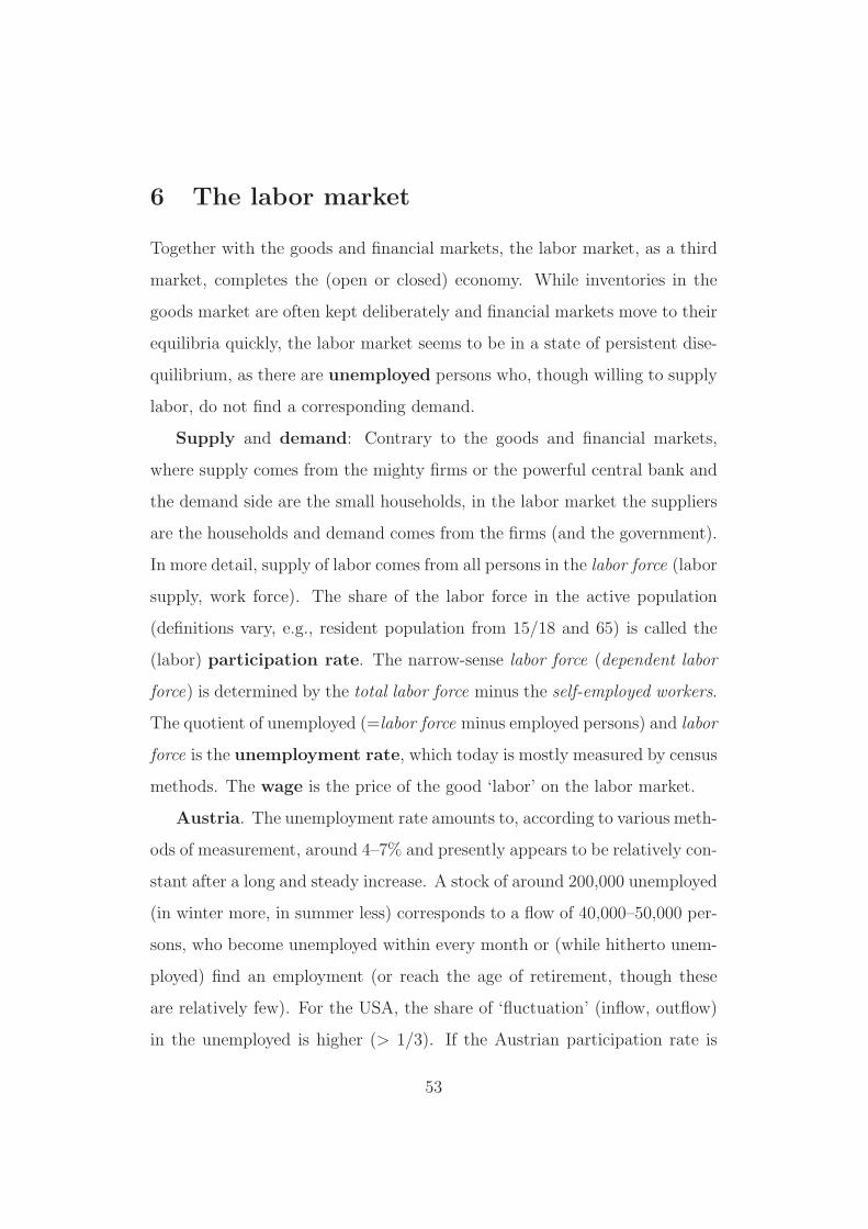
Austria. The unemployment rate amounts to, according to various meth-

ods of measurement, around 4–7% and presently appears to be relatively con-

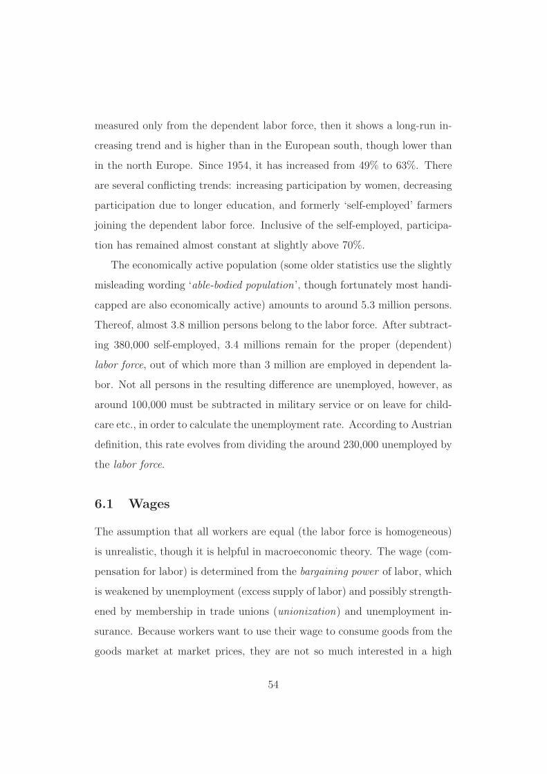
stant after a long and steady increase. A stock of around 200,000 unemployed

(in winter more, in summer less) corresponds to a flow of 40,000–50,000 per-

sons, who become unemployed within every month or (while hitherto unem-

ployed) find an employment (or reach the age of retirement, though these

are relatively few). For the USA, the share of ‘fluctuation’ (inflow, outflow)

in the unemployed is higher (> 1/3). If the Austrian participation rate is

53

measured only from the dependent labor force, then it shows a long-run in-

creasing trend and is higher than in the European south, though lower than

in the north Europe. Since 1954, it has increased from 49% to 63%. There

are several conflicting trends: increasing participation by women, decreasing

participation due to longer education, and formerly ‘self-employed’ farmers

joining the dependent labor force. Inclusive of the self-employed, participa-

tion has remained almost constant at slightly above 70%.

The economically active population (some older statistics use the slightly

misleading wording ‘able-bodied population’, though fortunately most handi-

capped are also economically active) amounts to around 5.3 million persons.

Thereof, almost 3.8 million persons belong to the labor force. After subtract-

ing 380,000 self-employed, 3.4 millions remain for the proper (dependent)

labor force, out of which more than 3 million are employed in dependent la-

bor. Not all persons in the resulting difference are unemployed, however, as

around 100,000 must be subtracted in military service or on leave for child-

care etc., in order to calculate the unemployment rate. According to Austrian

definition, this rate evolves from dividing the around 230,000 unemployed by

the labor force.

6.1 Wages

The assumption that all workers are equal (the labor force is homogeneous)

is unrealistic, though it is helpful in macroeconomic theory. The wage (com-

pensation for labor) is determined from the bargaining power of labor, which

is weakened by unemployment (excess supply of labor) and possibly strength-

ened by membership in trade unions (unionization) and unemployment in-

surance. Because workers want to use their wage to consume goods from the

goods market at market prices, they are not so much interested in a high

54

Figure 9: Austrian unemployment rate according to its traditional definition.

Figure 10: Inflows to and outflows from the stock of job vacancies in Austria

indicate the inflows and outflows from the stock of unemployed.

55

nominal wage W (money wage) as in a high real wage W/P .

The reservation wage is a wage rate, below which an unemployed per-

son is not willing to supply labor (a person unwilling to supply labor is not

necessarily just lazy; consider the fixed costs of employment, such as disci-

pline, clothing, costs of commute etc.). Even for a homogeneous work force,

firms often tend to pay higher wages than the reservation wage or a legally

determined minimum wage, in order to tie workers to the firm, to avoid

search costs, to enjoy the production effects of firm-specific training costs,

and to prevent shirking (sloppy work, bad workers’ morale). Such wages are

also called efficiency wages.

Efficiency wages. Blanchard’s definition of efficiency wages is a bit

unclear, as he introduces them as ‘linking wages to productivity’, which

is a general characteristic of all wages, as will be visible from the price-

determination mechanism below. The point is that workers’ productivity is

assumed to depend positively on their wages. This could explain why employ-

ers in some industries pay workers more than employers in other industries

do, even if the workers have apparently comparable qualifications and jobs.

[from a web dictionary]

As a wage function, one could use

W = P eF (u, z) (20)

where P e denotes the expected price level in the goods market, u is the unem-

ployment rate, z is used for ‘other influential variables in the labor market’

(Blanchard’s catchall variable), and the function F represents bargaining

power. The catchall z summarizes various effects. For example, increased

fluctuation to and from unemployment reduces the fear of unemployment,

even at rather high u, as it appears to be easier to find a job. Similarly,

unionization and unemployment insurance are expressed in z. Because the

56

wage is fixed in negotiations for a considerable time span (there is no contin-

uous bargaining process), W/P e is the expected real wage for the immediate

future. The function F is falling in u (unemployment weakens bargaining

power).

6.2 Prices

In Keynesian short-run models, prices are fixed and exogenous. If wages are

set, we must also be able to determine prices. If there is competition, a main

role is played by the production function, which indicates which amount

of input of production factors generate which amount of output. At first,

Blanchard uses the simple production function

Y = AN , (21)

where N is the labor input (‘employment’) and A is labor productivity.

A = Y/N indicates, how much output can be produced with one input unit

of labor. In the last 100 years, the ratio A has increased by a multiple. In

order to simplify the calculation, one may set A = 1 in the following, for

example by re-defining the unit of produced goods.

At perfect competition (microeconomics), it is known that prices and

wages must correspond to the marginal product of labor ∂Y/∂N = A. From

this one may derive that W = AP (per capita wage = price per unit of

output × goods produced by one worker) or W/P = A (real wage = labor

productivity) or even P = W/A (price = wage per unit of output). In real-

life economies, however, producers succeed in adding a mark up µ to wage

costs, such that

P = (1 + µ)W/A .

Here, W/A would be the wage rate per unit of produced good at competition,

57

as a worker produces A goods. µ can be viewed as a measure for the ‘market

power’ of firms, or as a compensation for other ‘production factors’ (capital,

energy, land). The simplifying assumption that A = 1 yields P = (1 + µ)W .

6.3 Prices and wages in equilibrium

In a (u,W/P )–diagram, one can draw the solution curve for the wage deter-

mination equationW

P= F (u, z)

for exogenous (fixed) z and for the assumption P = P e (price expectations

are fulfilled!). As already explained, this is a falling curve (in fact, it is a labor

supply function, which is positively sloped but drawn as negatively sloped,

as instead of employment the x–axis shows the unemployment rate u). In

this (u,W/P ) diagram, the price determination equation

W

P=

A

1 + µ

appears as a horizontal line (in principle, a labor demand function, which

should be negatively sloped or, in our diagram, positively sloped, but due to

the very simple production function with constant ‘returns to scale’ is flat).

The intersection of both curves implies an equilibrium real wage and an

equilibrium unemployment rate un. This unemployment rate is called the

natural unemployment rate, though it is no constant of nature, but is

rather determined by variables and parameters that express market power

or the technology, such as z and µ. Although wages and prices are in their

equilibrium, there is unemployment, i.e. the labor market does not ‘clear’.

Natural employment Nn is given by

Nn = L(1 − un)

58

if L denotes the labor force. Because of Y = AN , there is also a natural

output Yn, determined from

F (un, z) = F (1 −N

L, z) = F (1 −

Yn

AL, z) =

A

1 + µ

or, using the simplifying assumption A = 1

F (1 −Yn

L, z) =

1

1 + µ,

which determines Yn implicitly. Therefore, the natural output is that out-

put, at which there is natural unemployment and wages and prices are in

equilibrium.

Is there an equilibrium in the labor market? In the interpreta-

tion of Blanchard’s textbook, the labor market is in equilibrium whenever

price and wage determination coincide and when there is natural unemploy-

ment. Thus, in the short run the labor market is in a disequilibrium, in

the medium run it tends to its equilibrium. Alternatively, one might define

short-run equilibria at unemployment rates different from the natural rate,

or one may argue that the market is in equilibrium only when there is no

unemployment, excepting short episodes of job search. The text book uses a

possible compromise.

Does labor productivity A affect the natural unemployment

rate? In the price determination equation, higher A clearly raises the real

wage that firms are willing to pay. If the function F (u, z) remains constant,

u will decrease and the real wage increases. However, it is likely that A af-

fects the bargaining function, as workers demand for their share in the added

value of the productivity increase. In this case, un will re-increase, maybe

right to its former value. However, this is not a coercive consequence of the

model, as F (u, z) has been introduced simply as bargaining power and not

as labor supply.

59

Which economic variables affect the natural unemployment rate?

Remembering that un is defined implicitly as the solution of

F (un, z) =A

1 + µ,

we see that un is determined by: the markup µ, the catchall for factors

determining bargaining power z, the form of the bargaining-power function

F , and possibly productivity A. Conversely, no other economic variables

appear in this condition, such as: fiscal policy, monetary policy, consumer

sentiment, inflation and prices. The natural rate un is immune to any change

in any of these macroeconomic conditions.

60

7 The three markets jointly: AS and AD

Idea: The IS-LM model describes the short-run equilibrium on the goods

market and financial market, which presupposes that prices P are fixed and

that the short-run demand for goods creates its supply at current prices

(Y = Z). In the longer run, prices may move. The short-run equilibrium

Y of the nominal IS-LM model in the (Y, i) diagram need not coincide with

the ‘natural output’ Yn of the labor market. In the longer run, falling or

rising prices cause Y to converge to Yn. Blanchard calls the stage that is

attained in this section the ‘medium run’, in order to reserve the name ‘long

run’ for growth models.

In detail, Blanchard’s models use four different time horizons:

1. In the shortest run, prices P are fixed and thee price and wage deter-

mination in the labor market plays no role. Demand creates its own

supply, the narrow-sense IS-LM scheme holds.

2. In the short run, prices, wages, and employment may move but do not

necessarily coincide with their expectations P e. This time horizon is

treated by the AS-AD scheme. The goods supply is flexible, though

not entirely ‘endogenous’.

3. In the medium run, all expectations regarding prices are fulfilled. Nat-

ural employment and natural (potential) output determine an invariant

equilibrium. The goods supply is fixed.

4. In the long run, all determinants for the natural output are changeable.

This long run is the subject of growth theory, which, e.g., wants to

explain growth and welfare differentials between OECD and developing

countries.

61

7.1 The aggregate supply: the AS curve

AS is for aggregate supply. In the labor market, equilibrium is defined by

W = P eF (u, z)

P = W (1 + µ)

(A = 1 is retained). Inserting the first into the second equation yields

P = (1 + µ)P eF (u, z) = (1 + µ)P eF (1 −Y

L, z) (22)

For fixed µ, P e, z, L (and A), this defines a functional relation between P and

Y . For general A, one obtains

P =1 + µ

AP eF (1 −

Y

AL, z) .

Is this function increasing or decreasing?

If Y rises, there will also be higher employment N = Y (or, for the more

general form Y = AN analogously N = Y/A), therefore the unemployment

rate u falls, hence the functional value F (u, z) increases, as F is a falling

function of u (bargaining power). Thus, P rises. The function defined in

(22) is also increasing in a (Y, P ) diagram. It bears the name AS curve and

describes short-run equilibria in the labor market. It can, however, also be

interpreted as the quantity that is produced and supplied at a given price P

using the required amount of labor, when it is read inversely, with Y as a

function of P . Therefore, it is a genuine supply curve.

Attention: the AS curve derived here contains characteristics of imper-

fect markets, such as unsatisfied price expectations and mark-ups. Without

these characteristics, the equilibrium output would not depend on price and

the AS–curve would be vertical. Some economists think that the long-run

(Blanchard: medium-run) AS curve indeed is vertical. This ‘long-run AS

62

curve’ corresponds to the line Y = Yn. It will be shown that this is the only

longer-run equilibrium indeed.

The natural unemployment solves the AS curve for P = P e. If

prices equal their expectations, it holds that

P =1 + µ

APF (1 −

Y

AL, z)

or

F (1 −Y

AL, z) =

A

1 + µ,

which was the definition of natural output Yn. Similarly, 1−Yn/(AL) defines

the natural unemployment rate. The point (Yn, Pe) lies on the AS curve for

exogenously givens P e. From this and the positive slope of the AS curve, it

follows that:

1. If Y > Yn, then P > P e, or vice versa. Therefore, an ‘unnaturally’ large

output can be attained only when prices are higher than expected.

2. If Y < Yn, then P < P e, or vice versa. Therefore, an ‘unnaturally’ low

output occurs if prices are lower than expected.

7.2 The aggregate demand: the AD curve

The IS-LM model

Y = C(Y − T ) + I(Y, i) + G

M

P= Y L(i)

implies, for a given price P , a uniquely defined Y . If one increases P , then

the LM curve shifts leftward (already shown), such that higher prices imply

a higher i and a lower Y . Higher P therefore implies less output Y , as the

increased interest rate negatively affects investment demand and, by way of

63

the multiplier effects, decreases Y even further. Conversely, lower P means

higher output Y , due to the stronger investment and the multiplier effect.

In summary, one gets a falling curve in the (Y, P ) diagram, the AD curve

(aggregate demand). It is a genuine demand curve, as it describes (seen

inversely) the quantity in the goods market that is demanded at a given

price.

The negative slope of the AD curve is unequivocally accepted among

economists. For a given functional form and under certain assumptions, it

is mathematically feasible to solve the LM identity for the interest rate, to

substitute i in the IS function and then to solve for Y . In short, this implies

Y = Y (M

P,G, T ) ,

+ + −

as it is used by Blanchard. The prices are influential only by way of the

real money M/P . As M/P has a positive influence on Y , the price level in

the denominator has a negative effect on output, just as it should be.

7.3 Movements in the AS-AD world

What happens if Y at the intersection point of AS and AD exceeds

Yn? The labor market is not in its medium-run equilibrium, as u is less

than the natural un. The price expectations are not fulfilled, P > P e. By

a mechanism that is not described in the model, price expectations adapt to

actual prices. In the diagram, the AS curve experiences an upward shift.

(A possibility for a formal derivation would be the specification P et = Pt−1

suggested by Blanchard.) In the model, one might assume the following

sequence of events: higher wages are demanded; higher wages imply higher

prices via the markup (‘wage-price spiral’). An upward movement occurs on

64

the AD curve. Output has fallen, prices have risen. The game continues,

until Yn has been attained. There, the labor market is, at P = P e, in its

medium-run equilibrium.

What happens if an expansive monetary policy is pursued? We

know that this leads to a lower i and a higher output Y . Because a higher

output is implied at every P , the AD curve shifts to the right. Therefore, in

the AS-AD diagram, output and prices increase. Because of Yn < Y , there is

a pressure on the labor market to further increase wages and prices, and thus

formally to shift up the AS curve. As in the previous point, this development

stops when Y = Yn. Prices have, however, risen permanently, in 2 phases.

What happens if an expansive fiscal policy is pursued? Just the

same, except that, at first (in Phase 1), the interest rate rises instead of

falling. This ‘washes out’ private investment, and this feature continues to

work in Phase 2, when the AS curve shifts and prices increase once more.

Output finishes again at Yn, though with lower investment and higher G. A

similar effect is achieved by expansive fiscal policy via a tax cut, because of

the reaction of interest rates. Finally, output is at the same level as before

the tax cut, but investment has fallen and private consumption has increased,

and so has the price level.

What happens at restrictive fiscal policy? For example, assume

that government lowers its expenditure G. At first, this causes a contraction,

leading to lower Y at lower interest rate i. In the AS-AD diagram, the AD

curve has shifted left, P and Y have fallen. Because Y < Yn, there is higher

unemployment than un, wages and prices are reduced, the AS curve shifts

down. Wages and prices fall, until Y = Yn is attained. A lower price level

is obtained, at lower government expenditure. G has been substituted by

investment, which has increased because of the lower interest rate.

65

Conclusion. Expansionary policy can only be successful in the short run.

In the longer run, both fiscal and monetary policy are neutral with respect

to income. Contractive fiscal policy can have beneficial longer-run effects,

such as balancing the government budget and creating positive incentives for

private investment. How long it takes, until the economy will return to its

‘natural output’, cannot be stated exactly, a cycle of several years appears

to be realistic. During that phase, an expansive policy causes output to be

actually higher than natural output, thus economic policy has real effects.

Exogenous change of supply parameters. Both fiscal and monetary

policy cause, at first, shifts in the AD curve, which are neutralized in a 2.

phase by an opposite movement of the AS curve. As an example for an

autonomous shift of the AS curve, Blanchard names the OPEC shocks of

the 1970s, which he interprets as an increase in the markup µ. The upward

shift of the AS curve yields a decrease in Y at increasing prices. The graph

tells us that Y has not sufficiently fallen to match the new and much lower

natural output Yn. The disequilibrium in the labor market leads to a further

reduction of output at increasing prices, until Y = Yn.

For an exogenous change of price expectations P e or of the bargaining

position of labor suppliers z, one should be able to see similar movements.

In this case, the natural output changes, permanent effects occur.

Business cycles (business cycles, brit. also trade cycles) are fluctuations

in output that may be caused by diverse ‘shocks’ to aggregate supply or

demand. The idea is that output moves from peak to trough (‘recession’,

red light) and then from trough to peak (‘recovery’, green light), around an

unknown equilibrium or potential output. Contrary to their name, these

fluctuations are irregular rather than strictly cyclical.

66

8 The Phillips curve

In 1958, the economist Phillips drew, for British data, a (u, πw)–diagram

with wage inflation on the y–axis. The diagram showed a strong negative

correlation. Historically, the first report on such statistical relationships is

ascribed to Irving Fisher. Instead of wage inflation πw, later authors used

price inflation π and obtained similar patterns. Such a negative relation can

be derived from the AS curve

P = (1 + µ)P eF (u, z)

where, e.g., P e = Pt−1, i.e. expected prices equal those of the previous period

(of last year). We know that ∂F (u, z)/∂u < 0. By way of several mathemat-

ical approximation steps, one may derive that

πt = µ + zt − αut

with α > 0, or, at positive inflationary expectations πet , also

πt = πet + µ + zt − αut (23)

[The original Phillips curve was no linear function; Phillips did not se-

riously consider this possibility!] Such functions are also called ‘modified

Phillips curves’, more exactly ‘expectations-augmented Phillips curves’.

Derivation by linearization: Putting F (u, z) = 1 + z − αu yields for

P et = Pt−1

Pt

Pt−1

= (1 + µ)(1 + zt − αut) ,

πt =Pt − Pt−1

Pt−1

= µ + zt − αut .

Here it is assumed that µ, z, αu are ‘small’, such that all products of such

terms can be ignored, which justifies the approximative ‘=’ For general P et ,

67

one has analogously

Pt

Pt−1

=P e

t

Pt−1

(1 + µ)(1 + zt − αut) ,

πt = πet + µ + zt − αut .

Here the expected rate of inflation πet is defined by (P e

t − Pt−1)/Pt−1, i.e. by

the inflation that is expected in t − 1 for t. In the following ‘=’ will simply

be replaced by ‘=’, which is justified, as the form F (u, z) = 1 + z − αu was

assumed arbitrarily.

Conclusion: The rate of inflation πt tends to rise at higher inflationary

expectations, as the wage earners demand for a higher wage rise, to com-

pensate the price increases; it also rises at a higher markup, as then firms

will even add more to wages; it falls with higher unemployment, as the

bargaining power of workers drops; many more factors z affect this relation.

Evidence: While, for many years, the curve appeared to fit the data

well, it broke down in the 1970s (at least, this is what the text books say).

Friedman explained this disappearance by several factors :

1. The OPEC price shock led to additional inflation that was not rooted in

the price-wage spiral of the home economy. This implied high inflation

at rather high unemployment.

2. A closer view of the modified Phillips curve reveals that a negative

relationship is only possible when πet 6= πt. For ‘rational’ inflationary

expectations Et−1πt = πet , πt and πe

t only differ by an unsystematic

error, the values of u cluster around a ‘natural unemployment rate’,

notwithstanding the level of the (on average, correctly expected) infla-

tion. Trade unions, firms, wage earners learn sooner or later, how to

form expectations rationally.

68

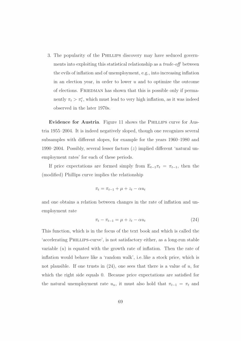
3. The popularity of the Phillips discovery may have seduced govern-

ments into exploiting this statistical relationship as a trade-off between

the evils of inflation and of unemployment, e.g., into increasing inflation

in an election year, in order to lower u and to optimize the outcome

of elections. Friedman has shown that this is possible only if perma-

nently πt > πet , which must lead to very high inflation, as it was indeed

observed in the later 1970s.

Evidence for Austria. Figure 11 shows the Phillips curve for Aus-

tria 1955–2004. It is indeed negatively sloped, though one recognizes several

subsamples with different slopes, for example for the years 1960–1980 and

1990–2004. Possibly, several lesser factors (z) implied different ‘natural un-

employment rates’ for each of these periods.

If price expectations are formed simply from Et−1πt = πt−1, then the

(modified) Phillips curve implies the relationship

πt = πt−1 + µ + zt − αut

and one obtains a relation between changes in the rate of inflation and un-

employment rate

πt − πt−1 = µ + zt − αut (24)

This function, which is in the focus of the text book and which is called the

‘accelerating Phillips-curve’, is not satisfactory either, as a long-run stable

variable (u) is equated with the growth rate of inflation. Then the rate of

inflation would behave like a ‘random walk’, i.e. like a stock price, which is

not plausible. If one trusts in (24), one sees that there is a value of u, for

which the right side equals 0. Because price expectations are satisfied for

the natural unemployment rate un, it must also hold that πt−1 = πt and

69

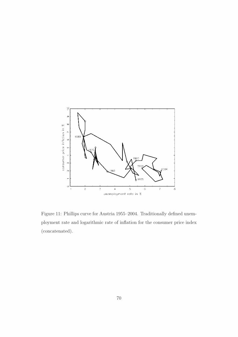
Figure 11: Phillips curve for Austria 1955–2004. Traditionally defined unem-

ployment rate and logarithmic rate of inflation for the consumer price index

(concatenated).

70

therefore u must equal un. Therefore, un is also called the NAIRU (non-

accelerating inflation rate of unemployment), as for this value the inflation

does not accelerate. In theory, the form of the accelerating Phillips-curve

implies a NAIRU of

un =µ + z

α.

Because, however, z is only a catchall variable without known numerical

value, one cannot really calculate the NAIRU from this formula. Adepts

of this specification can explain changes in the NAIRU by changes in the

mark-up µ or in the bargaining power of workers z.

Note. The NAIRU formula un = (µ + z)/α coincides with the natural

rate un as determined from F (u, z) = 1/(1+µ), if one uses the approximation

1 − µ = 1/(1 + µ), which is valid for a small mark-up µ.

Empirical evidence. For Austria, the accelerating Phillips curve

leaves a rather sad impression. A systematic negative relationship is not

visible. Note the year 1984, when the rate of inflation experienced a strong

short-term increase because of an increase in the value added tax rate on

luxury goods. A medium-run constant NAIRU cannot be calculated from

such data. Some economists assume stronger fluctuations in the NAIRU (in

the Blanchard model, such fluctuations would follow from changes in µ

and z), which however weakens the significance of the whole concept.

A compromise. If price expectations are assumed to follow the specifi-

cation πet = θπt−1, one obtains the modified Phillips curve

πt = θπt−1 + µ + zt − αut .

In this model, there is a trade-off between inflation and unemployment, which

is however much weaker than in the classical Phillips curve. Blanchard

interprets the disappearance of the US Phillips curve as an increase in θ

71

Figure 12: Accelerating variant of the Phillips curve for Austria during the

years 1955–2004.

72

from nearly 0 to nearly 1. A statistical regression estimation for Austrian

data yields a θ of around 0.6. A different interpretation of θ views this para-

meter as the share or intensity of indexed wage contracts. Such indexation

plays a strong role during episodes of hyperinflation: if wages are indexed to

the current rate of inflation, then θ can be greater 1. Others see in θπt−1 a

‘core inflation’, which does not necessarily coincide with πet .

Summary: Out of the AS–curve, which plots prices against output (or

the unemployment rate), Phillips created the Phillips curve, which plots

price inflations against u, even later followed a variant of the Phillips-curve,

which plots growth rates of price inflation against u. In summary, a deviation

from the natural rate un, or the NAIRU, can only be achieved, if prices

increase more strongly than it was assumed by workers who negotiate their

wages and thus their targeted real wage is not satisfied, such that workers

are cheated upon. This is, of course, not systematically possible.

8.1 Okun’s law

Apart from the Phillips curve, another empirical relationship enjoys great

popularity among empirical macroeconomists, the so-called Okun’s law. There

is an exact one-one correspondence between natural output Yn and the nat-

ural unemployment rate un because of un = 1 − Yn/L. Therefore, it would

be interesting to know how strongly deviations from natural output are re-

flected in deviations from the natural unemployment rate. A formula due to

the economist Okun was

3(un − u) =Y − Yn

Yn

(25)

Both sides are measured in percentages (%). If the unemployment rate is one

percentage point below the NAIRU, then output will be 3% above natural

73

output (or potential output).

Today, this function is usually presented in a modified form:

ut − ut−1 = −β(gt − gn) (26)

Here, gt denotes the actual growth rate of real output, while gn is its ‘natural’

growth rate. The equation assumes that, instead of ‘natural output’, there

is a natural growth rate gn, which should be around 2-3%. If output grows

at g > gn, then the unemployment rate falls. If the unemployment rate in

t − 1 exactly matches the NAIRU, then it falls below the NAIRU in t. If

output (the real GDP) grows slower than gn, then the unemployment rate

rises above the NAIRU. Most authors find that β > 0 is around 0.4.

Where does β come from? At low flexibility of the labor market, at

high costs of hiring and firing (adaptation costs), it may be rational for the

firms to meet an increased demand for goods with overtime work instead of

new hirings of workers and, conversely, to ‘hoard’ workers if demand is low.

Then, β will be low. If the costs of labor mobility decrease, β will rise. Many

economists find that β has increased in the last 20-30 years.

Where does the natural growth rate come from? From the growth

of labor productivity. If the same input of labor can produce more goods,

output must increase more strongly, if it should generate an additional de-

mand for labor.

Evidence for Austria: For Austria, the evidence on the existence of

Okun’s law, in the above indicated form, remains unconvincing. Whereas,

on average, years with good economic performance indeed have lower unem-

ployment than years of economic slump, the autonomous developments in

the labor market dominate: the decline in the work force of the Austrian

industry, or rather a strong surge in labor productivity, 1980–1990, and the

stabilization of unemployment in the following years in spite of moderate

74

economic performance. Comparative country studies confirm that Austria is

an exception.

Note. Okun’s law focuses on growth rates. These are the main subject

of so-called growth theory, which addresses long-run economic developments.

The natural growth rate (e.g. 3%) is sometimes derived informally by con-

sidering a simple production function such as Y = AN . Then, if the labor

force L, and in consequence also N , grows at 1%, the labor productivity A at

2%, then output should grow at 3%. In economic reality, structural changes,

other production factors (e.g. capital) etc. play a non-negligible role.

8.2 Growth of money and inflation

Blanchard closes his medium-run model, which contains a Phillips curve

in a debatable variant in differences

πt − πt−1 = −α(ut − un) , (27)

and an Okun’s law

ut − ut−1 = −β(gt − gn) , (28)

by a third equation that relates growth rates. This equation is derived from

the AD curve

Y = Y (M

P,G, T )

by simplification

Y = Y (M

P)

and by using a linear functional specification

Y = γM

P.

This yields, for constant γ, the relationship among growth rates

gY,t = gM,t − gP,t = gM,t − πt , (29)

75

as growth rates obey the same rules as logarithms. Here, π is the growth of

prices, i.e. inflation. The growth rate of Y is written in a clearer notation as

gY , while it is denoted by g in Okun’s law.

From the three relationships, one sees that an equilibrium is obtained if

ut = un and gt = gn. Then π does not change any more, the level of inflation

is determined by the expansion path of money supply. In theory, one could

choose gM = gt and thus achieve simply π = 0.

Growth rates and logarithms. If it holds that

Z = XY ,

then this implies that

log Z = log X + log Y .

If the 3 variables depend on time, this equation can be differenced with

respect to time t:

d log Z

dt=

d log X

dt+

d log Y

dtdZ/dt

Z=

dX/dt

X+

dY/dt

Y(30)

These would be growth rates in ‘continuous time’, i.e. if time passes contin-

uously, not in jumps or intervals. For the usual discrete-time growth rates

gZ,t =Zt − Zt−1

Zt−1

, (31)

the formula gZ = gX + gY holds approximately only. In the longer run,

however, the time interval from t to t+1 is comparatively small, so one may

work with the approximation.

Usage of the dynamic model. The three-equations model can be used

to describe a process of disinflation. Starting from an equilibrium situation

76

with u = un and g = gn and therefore gM = gn + πh for some πh, political

forces—obviously forces in control of the money supply and therefore rather

central banks than government agencies—wish to reduce π to a lower level πl.

In order to do so, they reduce gM . An option would be gM = gn + πl, which

can be adopted immediately and, in consequence, yields high unemployment

and low growth for a while, until eventually the new equilibrium is attained,

which is characterized by u = un, g = gn, and π = πl. Alternatively, one

could decrease gM gradually. Blanchard demonstrates that the sacrifice

ratio, i.e. the ratio of additional unemployment beyond un (measured in ac-

cumulated percentage points and years) divided by the disinflation πh −πl is

independent of whether the policy is gradual or immediate. This theorem is

true for most variants of these dynamic linear models, though not for all of

them.

77

9 The open economy

Contrary to the closed economy, the open economy communicates with the

rest of the world. It does so on three markets:

1. goods market (foreign trade): goods and (primarily touristic) ser-

vices are exported and imported. The idea that exports are good while

imports however are bad, insinuates restricting the free trade across

borders. Customs correspond to indirect taxes (goods taxes) on im-

ported goods and increase their prices (relative to domestic produc-

tion), quotas (rationing) limit the imported quantity of certain goods.

International tendency toward abolition of all restrictions on goods

trade.

2. financial market (capital mobility): bonds, shares, and other do-

mestic securities are bought by non-residents, then interest and div-

idends are paid to non-residents. Austrians buy, e.g., foreign shares

and receive dividends from abroad. Increasing international tendency

toward abolition of all restrictions on such action.

3. labor market: international wage differentials cause migration (im-

migration = inward migration, emigration = outward migration) and

the re-allocation of productive capital to countries with a low wage

level. In the EU-15 area (in theory) no restriction, worldwide strict

limits on migration.

The increasing openness of economies has advantages (higher welfare by

international division of labor) and disadvantages (loss of national auton-

omy, above all, of economic policy, ‘exposure’ to international crises). Most

economists agree that advantages dominate by far.

78

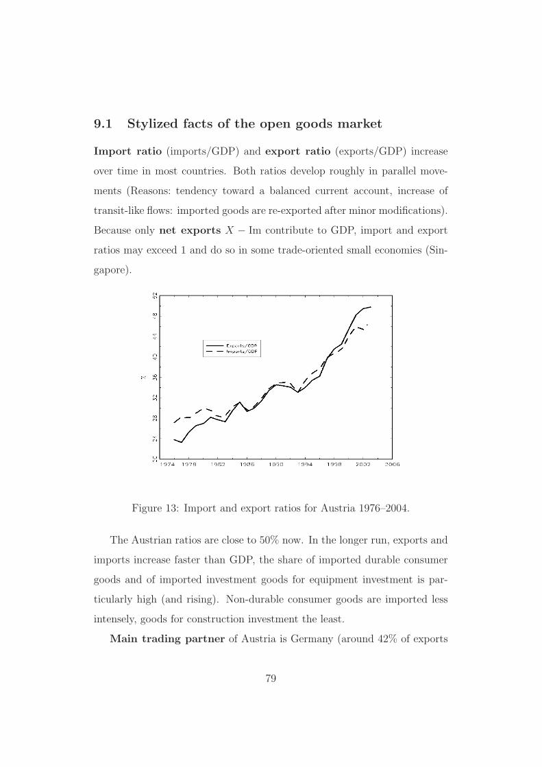
9.1 Stylized facts of the open goods market

Import ratio (imports/GDP) and export ratio (exports/GDP) increase

over time in most countries. Both ratios develop roughly in parallel move-

ments (Reasons: tendency toward a balanced current account, increase of

transit-like flows: imported goods are re-exported after minor modifications).

Because only net exports X − Im contribute to GDP, import and export

ratios may exceed 1 and do so in some trade-oriented small economies (Sin-

gapore).

Figure 13: Import and export ratios for Austria 1976–2004.

The Austrian ratios are close to 50% now. In the longer run, exports and

imports increase faster than GDP, the share of imported durable consumer

goods and of imported investment goods for equipment investment is par-

ticularly high (and rising). Non-durable consumer goods are imported less

intensely, goods for construction investment the least.

Main trading partner of Austria is Germany (around 42% of exports

79

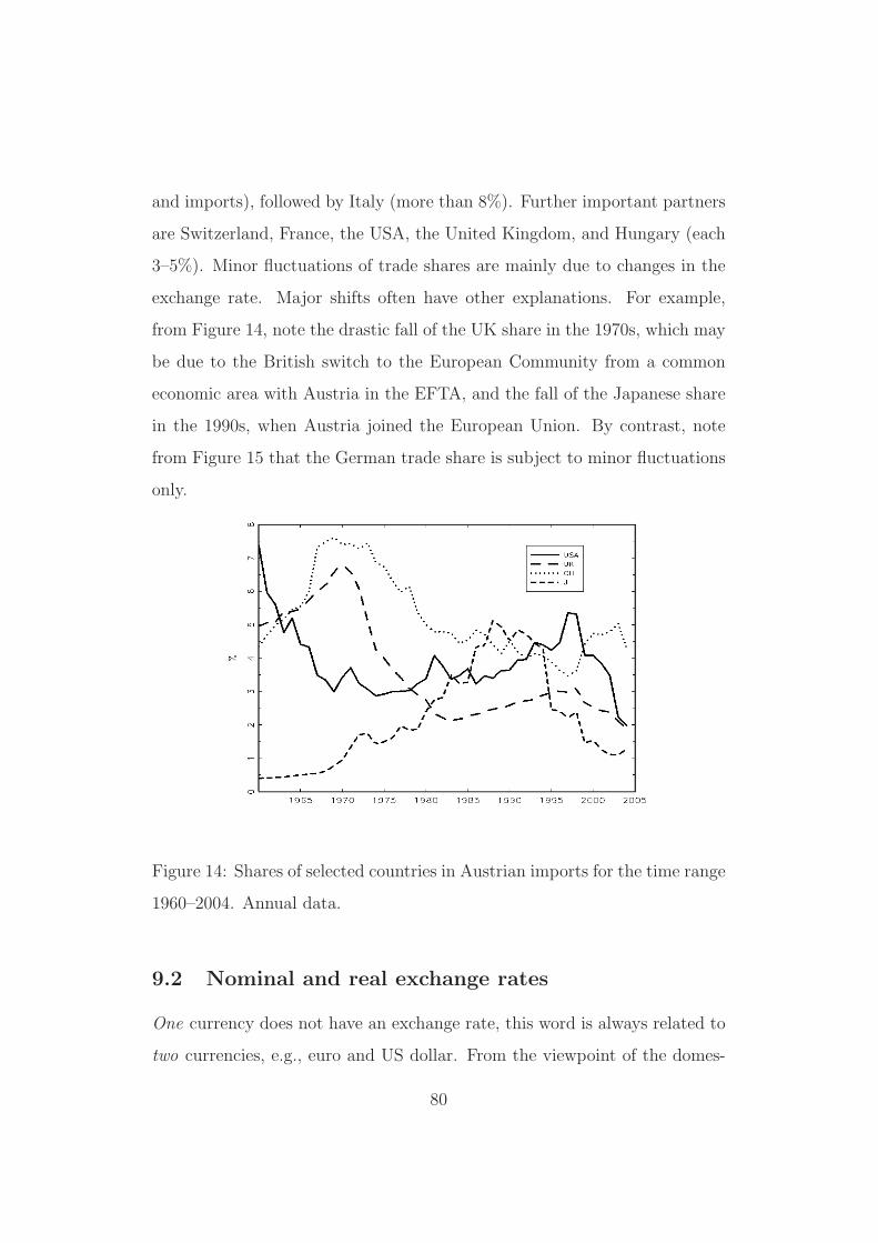
and imports), followed by Italy (more than 8%). Further important partners

are Switzerland, France, the USA, the United Kingdom, and Hungary (each

3–5%). Minor fluctuations of trade shares are mainly due to changes in the

exchange rate. Major shifts often have other explanations. For example,

from Figure 14, note the drastic fall of the UK share in the 1970s, which may

be due to the British switch to the European Community from a common

economic area with Austria in the EFTA, and the fall of the Japanese share

in the 1990s, when Austria joined the European Union. By contrast, note

from Figure 15 that the German trade share is subject to minor fluctuations

only.

Figure 14: Shares of selected countries in Austrian imports for the time range

1960–2004. Annual data.

9.2 Nominal and real exchange rates

One currency does not have an exchange rate, this word is always related to

two currencies, e.g., euro and US dollar. From the viewpoint of the domes-

80

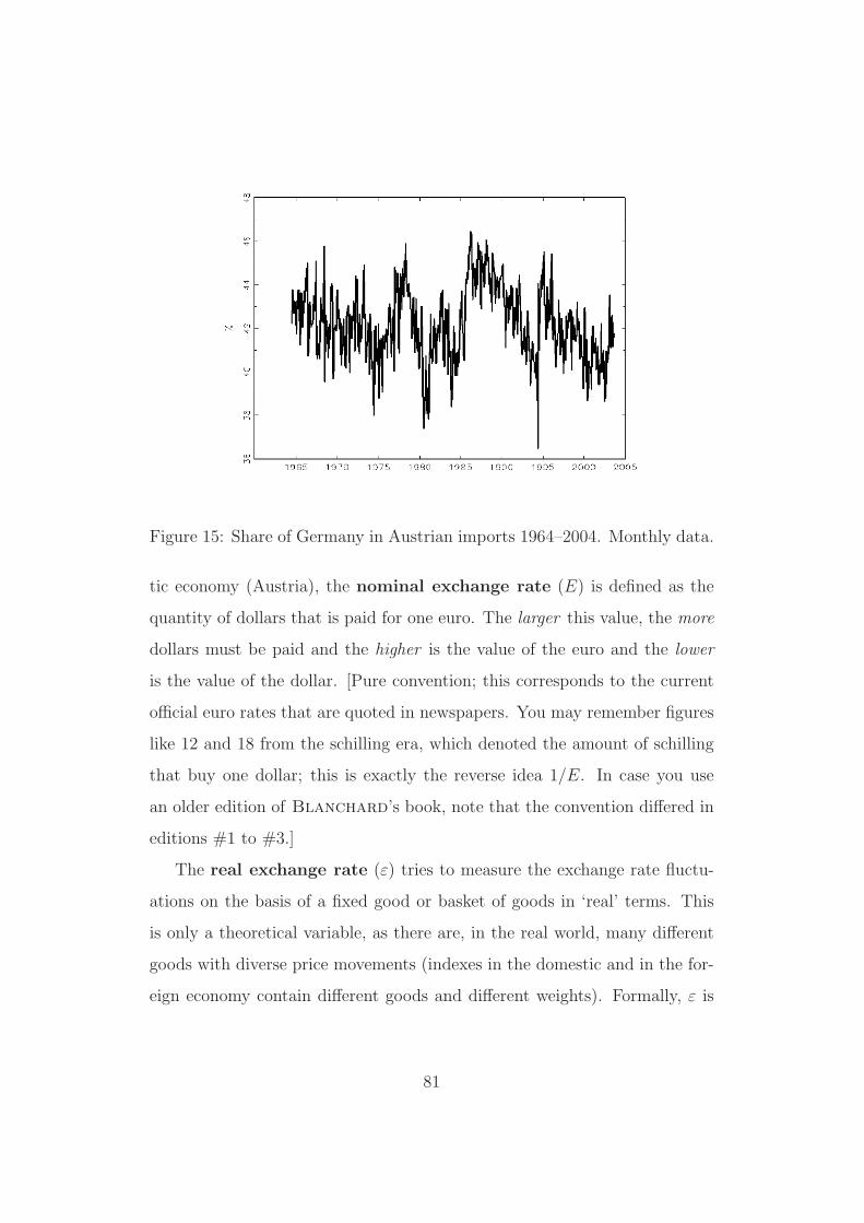
Figure 15: Share of Germany in Austrian imports 1964–2004. Monthly data.

tic economy (Austria), the nominal exchange rate (E) is defined as the

quantity of dollars that is paid for one euro. The larger this value, the more

dollars must be paid and the higher is the value of the euro and the lower

is the value of the dollar. [Pure convention; this corresponds to the current

official euro rates that are quoted in newspapers. You may remember figures

like 12 and 18 from the schilling era, which denoted the amount of schilling

that buy one dollar; this is exactly the reverse idea 1/E. In case you use

an older edition of Blanchard’s book, note that the convention differed in

editions #1 to #3.]

The real exchange rate (ε) tries to measure the exchange rate fluctu-

ations on the basis of a fixed good or basket of goods in ‘real’ terms. This

is only a theoretical variable, as there are, in the real world, many different

goods with diverse price movements (indexes in the domestic and in the for-

eign economy contain different goods and different weights). Formally, ε is

81

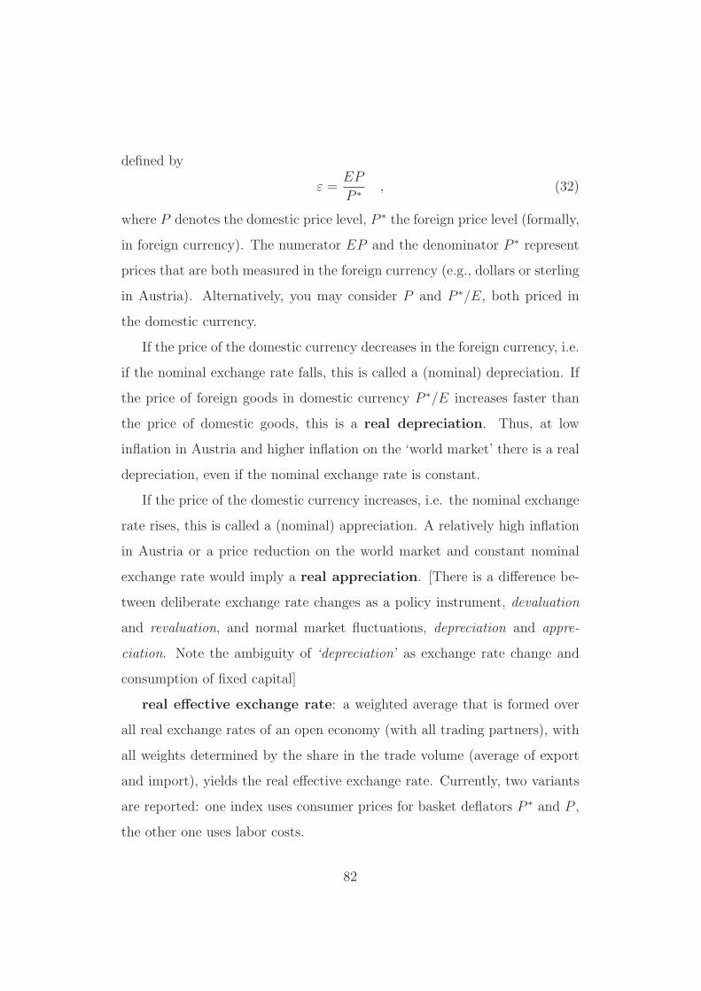
defined by

ε =EP

P ∗

, (32)

where P denotes the domestic price level, P ∗ the foreign price level (formally,

in foreign currency). The numerator EP and the denominator P ∗ represent

prices that are both measured in the foreign currency (e.g., dollars or sterling

in Austria). Alternatively, you may consider P and P ∗/E, both priced in

the domestic currency.

If the price of the domestic currency decreases in the foreign currency, i.e.

if the nominal exchange rate falls, this is called a (nominal) depreciation. If

the price of foreign goods in domestic currency P ∗/E increases faster than

the price of domestic goods, this is a real depreciation. Thus, at low

inflation in Austria and higher inflation on the ‘world market’ there is a real

depreciation, even if the nominal exchange rate is constant.

If the price of the domestic currency increases, i.e. the nominal exchange

rate rises, this is called a (nominal) appreciation. A relatively high inflation

in Austria or a price reduction on the world market and constant nominal

exchange rate would imply a real appreciation. [There is a difference be-

tween deliberate exchange rate changes as a policy instrument, devaluation

and revaluation, and normal market fluctuations, depreciation and appre-

ciation. Note the ambiguity of ‘depreciation’ as exchange rate change and

consumption of fixed capital]

real effective exchange rate: a weighted average that is formed over

all real exchange rates of an open economy (with all trading partners), with

all weights determined by the share in the trade volume (average of export

and import), yields the real effective exchange rate. Currently, two variants

are reported: one index uses consumer prices for basket deflators P ∗ and P ,

the other one uses labor costs.

82

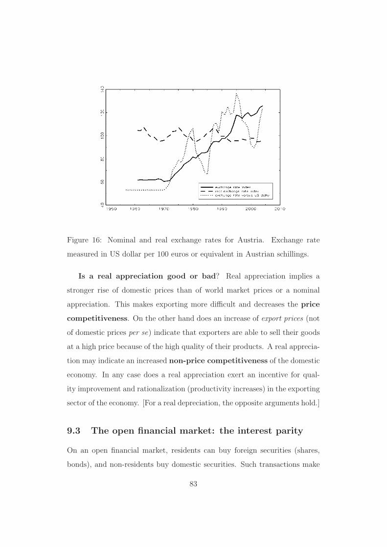
Figure 16: Nominal and real exchange rates for Austria. Exchange rate

measured in US dollar per 100 euros or equivalent in Austrian schillings.

Is a real appreciation good or bad? Real appreciation implies a

stronger rise of domestic prices than of world market prices or a nominal

appreciation. This makes exporting more difficult and decreases the price

competitiveness. On the other hand does an increase of export prices (not

of domestic prices per se) indicate that exporters are able to sell their goods

at a high price because of the high quality of their products. A real apprecia-

tion may indicate an increased non-price competitiveness of the domestic

economy. In any case does a real appreciation exert an incentive for qual-

ity improvement and rationalization (productivity increases) in the exporting

sector of the economy. [For a real depreciation, the opposite arguments hold.]

9.3 The open financial market: the interest parity

On an open financial market, residents can buy foreign securities (shares,

bonds), and non-residents buy domestic securities. Such transactions make

83

part of the capital accounts. If non-residents buy many domestic assets, a

passive (negative) trade balance and also current account balance may be

offset.

‘Arbitrage condition’: A domestic and a foreign bond are held at the

same time, only if both promise the same return. Otherwise all bond-holders

would only stock the asset that has the higher return. The expected return

is composed of the expectations for the exchange rate and the interest. For

a formula, one has

1 + it = Et(1 + i∗t )1

Eet+1

, (33)

the so-called uncovered interest parity (UIP). The left-hand side describes

the interest on a domestic bond. The right-hand side describes the behavior

of a bond-holder, who first purchases foreign currency, then receives the

interest on the foreign security, and finally changes back the total amount

into domestic currency. The latter transaction includes a risk, as next year’s

exchange rate is unknown today, hence the expected exchange rate Ee is

substituted. The UIP implies

i∗t = itEe

t+1

Et

+Ee

t+1 − Et

Et

Unless the expected change in the exchange rate is extremely large, the fac-

tor Eet+1/Et remains close to 1 and is often ignored to simplify the formula

somewhat, such that the approximation of the UIP

it=i∗t −Ee

t+1 − Et

Et

is often used.

Expected depreciation of the domestic currency causes a negative ratio

(Eet+1−Et)/Et and thus a relatively higher interest in the domestic economy,

expected appreciation means a higher interest abroad. In some countries

84

with a strong expectation of depreciation, the relation is seemingly violated,

as there an even higher return must be offered to compensate for the high

risk of such bonds.

9.4 The open goods market

In an open economy, the demand for domestic goods is given by

Z = C + I + G − Im/ε + X (34)

with exports X and imports Im. The correction factor 1/ε indicates that

foreign goods in imports Im differ from domestic goods in their value. In the

National Accounts, of course, Im/ε is booked as ‘real imports’.

Domestic demand C + I + G follows the hitherto used pattern

C(YD) + I(Y, r) + G (35)

The import function (import demand)

Im = Im(Y, ε) (36)

(+, +)

lets imports depend positively on domestic demand, without decomposition

into imports by particular demand categories, and positively on the real

exchange rate. The latter reaction stems from the fact that, at a higher ε,

foreign goods are relatively cheaper and tend to substitute domestic goods.

The export function (export demand)

X = X(Y ∗, ε) (37)

(+,−)

85

lets exports depend positively on foreign demand Y ∗ (demand on the world

market), and negatively on the real exchange rate, as a real depreciation

makes exported goods cheaper and more competitive.

Note that imports depend positively on income, while exports do not

react to Y . Therefore, at low Y net exports NX = X − Im/ε are positive,

and at high Y net exports are negative. Therefore, to every given ε there

is an income YTB, at which the trade balance is exactly equalized. This

YTB need not correspond to the equilibrium on the domestic goods market.

For example, it seems that the US goods market is in its equilibrium at a

passive trade balance, i.e. the domestic economy demands more than YTB −

NX(YTB). Currently, the Austrian foreign trade may be balanced.

Thought experiment 1: Increase of demand.

1. Increase of G (expansionary fiscal policy) raises imports Im/ε, how-

ever not by not the same amount. Therefore, higher Y results, with

multiplier effects in I and C likewise reflected in imports. Y increases,

X does not change, Im/ε increases, while NX falls. Therefore, the

trade balance becomes more passive. A part of the multiplier effect is

satisfied by imported goods.

2. Increase of foreign demand Y ∗ raises exports X. Although the addi-

tional demand in NX and thus in Y is satisfied partly by imports,

there remains a positive net effect. The trade balance becomes more

active, income increases.

Conclusion: An increased foreign demand is good, an increased domestic

demand is bad for the trade balance. [Every foreign economy is, however,

also a domestic economy]

Thought experiment 2: Devaluation.

86

At given fixed prices in the domestic economy (P ) and in the foreign econ-

omy (P ∗), a nominal depreciation causes a real depreciation (ε decreases).

Because of

NX = X − Im/ε = X(Y ∗, ε) − Im(Y, ε)/ε,

the net effect of a depreciation on net exports and thus on Y is uncertain.

Exports tend to increase and imports tend to decrease: these two effects tend

to increase NX. However, imports become more expensive, as 1/ε increases,

and this effect tends to decrease NX. The condition by Marshall-Lerner

tells that the net effect is positive. Most economists agree that this condition

is fulfilled for most countries.

Conclusion: a depreciation together with a restrictive fiscal policy leads

to the (sometimes desired) disappearance of a trade deficit and to constant

Y at reduced domestic demand. Should work in theory.

Dynamics: Because the contrary direct effect of ε in the equation for

NX occurs immediately, while the effects on export demand abroad and on

import demand in the home economy occur with a delay, after a depreciation

one often observes at first a fall in net exports (imports become more expen-

sive immediately) and then a gradual increase, according to Marshall-

Lerner beyond the starting value. Some economists see the letter ‘J’ in

this reaction, and they call this effect the J curve. The time range to an

improvement in the trade balance appears to last up to one year.

9.5 Investment and saving in an open economy

In a closed economy, the simple identities SH + T − G = I or SH + SP = I

hold. In an open economy, it follows from the identity

Y = C + I + G − Im/ε + X

87

after subtraction of C + T on both sides that

Y − C − T = SH = I + G − T − Im/ε + X

or

SH + SP − NX = I .

Investment equals the sum of 3 positions: household saving, government

saving, and the negative trade balance. The third position expresses financing

of investment by net imports and therefore by foreign debt.

Conclusion: Countries with a high household-saving rate and budget

surplus either have a positive trade balance or invest very much. A higher

budget deficit is either compensated by more household saving, less invest-

ment, or a deficit in the trade balance.

Even this identity is an ex post–identity only and does not describe a

behavioral mechanism. For example, it is not recognizable that a depreciation

or appreciation indeed affect the trade balance, although it seems that NX

is defined by SH + SP − I. The change of ε implies a change in demand and

affects both SH and I.

9.6 The IS-LM–model in the open economy

Mundell-Fleming model. The analysis of economic policy in an open

economy on the basis of the IS-LM diagram with the cases of flexible and fixed

exchange rates is due to Mundell (Nobel prize) and Fleming. Besides the

usual (Y, i) diagram, one often uses (not in Blanchard) the representation

in the (Y,E)–world.

While the LM equation of the closed economy

M

P= Y L(i)

88

continues to hold in the open economy, there are important changes to the

IS equation for equilibria in the goods market (for simplification, written in

the nominal interest rate i, i.e. for πe = 0)

Y = C(Y − T ) + I(Y, i) + G + NX(Y, Y ∗, ε)

and there is the interest parity (in the exact form)

Et =1 + it1 + i∗t

Eet+1

At a given expected exchange rate Eet+1 = Ee, one may express E as

E =1 + it1 + i∗t

Ee. (38)

Assuming additionally that, at least in the short run, P and P ∗ do not move,

one may substitute this expression for the (nominal) exchange rate instead

of the real exchange rate in the IS equation:

Y = C(Y − T ) + I(Y, i) + G + NX(Y, Y ∗,1 + i

1 + i∗Ee)

and one obtains a negatively sloped IS curve in the (Y, i) diagram. Because

a higher interest rate negatively affects both investment and net exports (i

is in the numerator of the last expression, E and therefore ε increases and

thus NX falls by ‘appreciation’), one may think that the curve would be

‘flatter’ than in a closed economy and monetary policy would have stronger

effects. The intersection of the LM and IS curve does not only determine an

equilibrium pair (Y, i), but also an equilibrium exchange rate.

fiscal policy in the open economy. The change in public demand

causes a shift of the IS curve at a rigid LM curve. For example, expan-

sionary fiscal policy. Both Y and i rise. The higher interest rate causes an

appreciation because of (38), i.e. E increases. In summary, private consump-

tion increases (depends directly on Y ), while the behavior of investment is

89

uncertain (higher Y , but also higher i), and net exports fall (Marshall-

Lerner). In other words, the trade balance deteriorates.

Monetary policy in the open economy. The change in the money

supply causes a shift of the LM curve at rigid IS curve. For example, expan-

sionary monetary policy. Y rises, but i falls. The lower interest rate causes

a depreciation, E falls. Private consumption, investment, and net exports

increase. This apparently ideal case includes, of course, the risk of inflation.

Fixed exchange rate. For diverse reasons, e.g., to eliminate exchange

rate risk, it may seem attractive to keep the nominal exchange rate E fixed.

The UIP determines the interest rate i uniquely, as i∗ and Ee are exogenous.

Therefore, at a fixed exchange rate there is no independent monetary policy

any more, this policy instrument is no more available. Because E and Ee

must coincide in the longer run, one sees from the UIP that i = i∗ must

hold, i.e. there is only one ‘international’ interest rate. The advantages of a

fixed exchange rate, such as easing of border-crossing trade with its welfare-

increasing effect, must be gauged against the disadvantage of abandoning

monetary policy as an instrument of economic policy.

Narrow-sense model cases of Mundell-Fleming. While in the

Blanchard variant with flexible exchange rate, the expected exchange rate

Ee is exogenous and fixed, which entails certain logical problems, Mundell-

Fleming assume in the simplest case Ee = Et, which implies i = i∗, also

for a flexible exchange rate. Then, one may draw IS and LM curves in the

(Y,E)–world.

1. With flexible exchange rates, the LM curve becomes vertical, as

i = i∗ and the exogenous money supply determines Y uniquely. The

IS curve is negatively sloped, because of the influence of net exports

and the Marshall-Lerner–condition. Fiscal policy is ineffective and

90

only affects the exchange rate. Monetary policy changes output di-

rectly.

2. With fixed exchange rates, the LM curve disappears, as the money

supply is set endogenously, such that the exchange rate is maintained

The IS curve continues to be negatively sloped and intersects a horizon-

tal E = E–line. Fiscal policy changes output directly, while monetary

policy is no more possible.

91