Introduction to Machine Learning

Reading for today: R&N 18.1-18.4

Next lecture: R&N 18.6-18.12, 20.1-20.3.2

Outline

• The importance of a good representation• Different types of learning problems• Different types of learning algorithms• Supervised learning

– Decision trees– Naïve Bayes– Perceptrons, Multi-layer Neural Networks– Boosting

• Unsupervised Learning– K-means

• Applications: learning to detect faces in images• Reading for today’s lecture: Chapter 18.1 to 18.4 (inclusive)

You will be expected to know

Understand Attributes, Error function, Classification, Regression, Hypothesis (Predictor function)

What is Supervised Learning?

Decision Tree Algorithm

Entropy

Information Gain

Tradeoff between train and test with model complexity

Cross validation

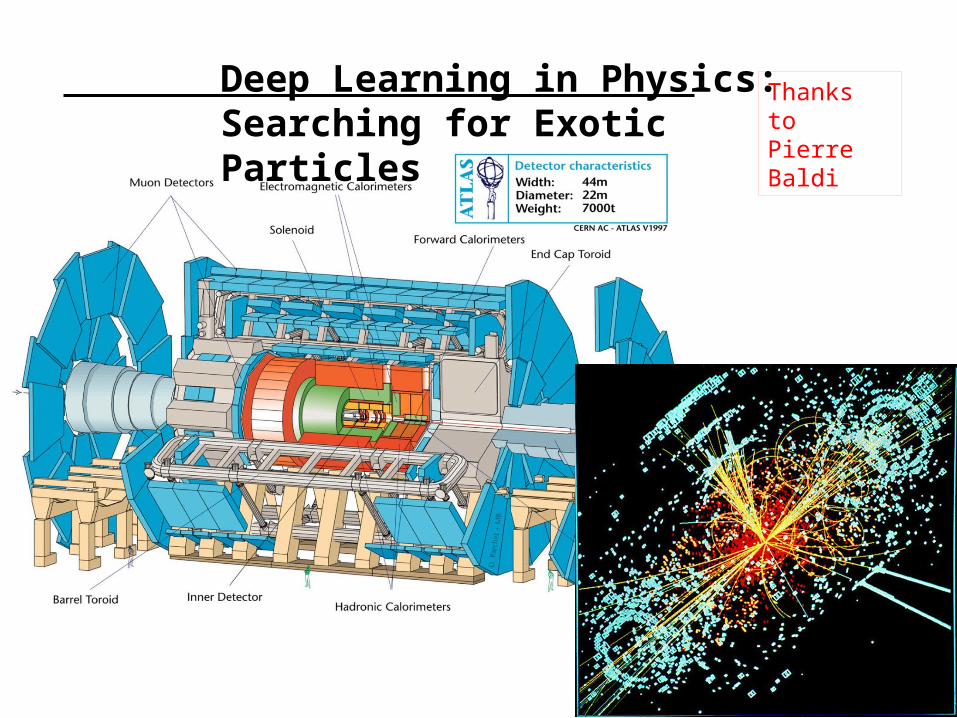
Deep Learning in Physics: Searching for Exotic Particles

Thanks to Pierre Baldi

Thanks to Pierre Baldi

Daniel Whiteson

Peter Sadowski

Thanks to Pierre Baldi

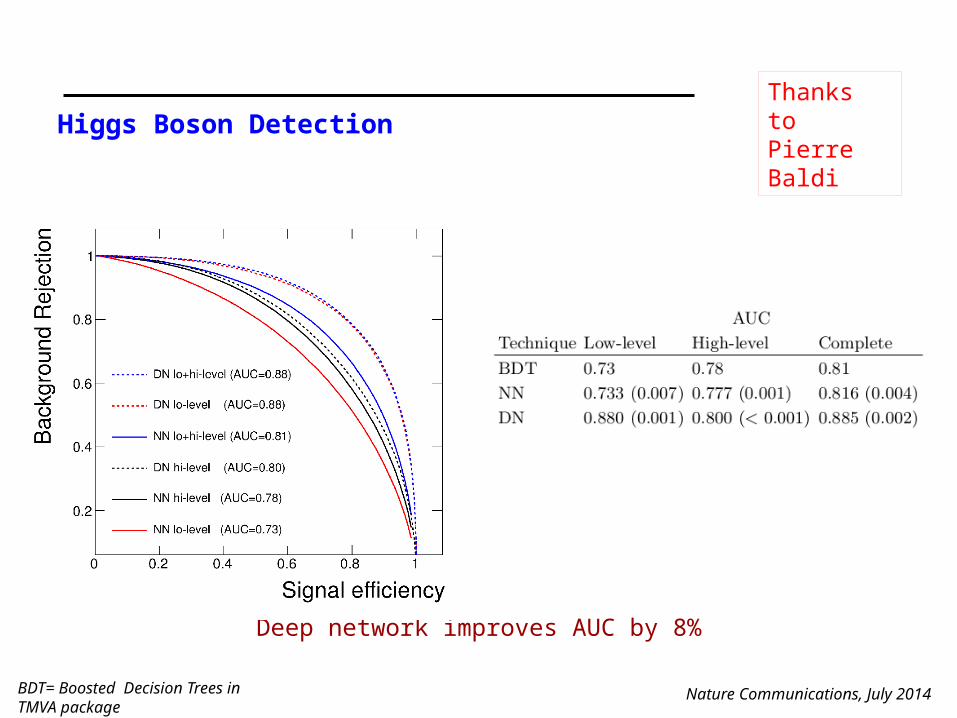
Higgs Boson Detection

Deep network improves AUC by 8%

Nature Communications, July 2014BDT= Boosted Decision Trees in TMVA package

Thanks to Pierre Baldi

Application to Extra-Tropical Cyclones

Gaffney et al, Climate Dynamics, 2007

Thanks to Padhraic Smyth

Iceland Cluster

Horizontal ClusterGreenland Cluster

Original Data

Thanks to Padhraic Smyth

Cluster Shapes for Pacific Typhoon Tracks

Camargo et al, J. Climate, 2007

Thanks to Padhraic Smyth

© Padhraic Smyth, UC Irvine: DS 06 11

TROPICAL CYCLONES Western North Pacific

Camargo et al, J. Climate, 2007

Thanks to Padhraic Smyth

An ICS Undergraduate Success Story

The key student involved in this work started out as an ICS undergrad. Scott Gaffney took ICS 171 and 175, got interested in AI, started to work in my group, decided to stay in ICS for his PhD, did a terrific job in writing a thesis on curve-clustering and working with collaborators in climate science to apply it to important scientific problems, and is now one of the leaders of Yahoo! Labs reporting directly to the CEO there, http://labs.yahoo.com/author/gaffney/. Scott grew up locally in Orange County and is someone I like to point as a great success story for ICS. --- From Padhraic Smyth

Thanks to Padhraic Smyth

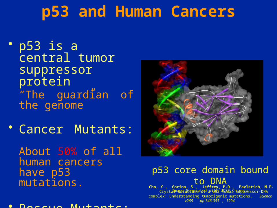
• p53 is a central tumor suppressor protein“The guardian of the genome”

• Cancer Mutants: About 50% of all human cancers have p53 mutations.

• Rescue Mutants: Several second-site

mutations restore functionality to some p53 cancer mutants in vivo.

p53 core domain bound to DNA

Image Generated with UCSF ChimeraCho, Y.,  Gorina, S.,  Jeffrey, P.D.,  Pavletich, N.P. Crystal

structure of a p53 tumor suppressor-DNA complex: understanding tumorigenic mutations. Science v265 pp.346-

355 , 1994

p53 and Human Cancers

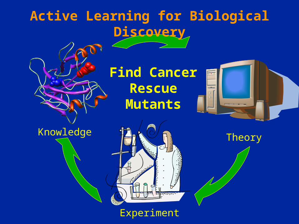
Theory

Find Cancer Rescue Mutants

Knowledge

Experiment

Active Learning for Biological Discovery

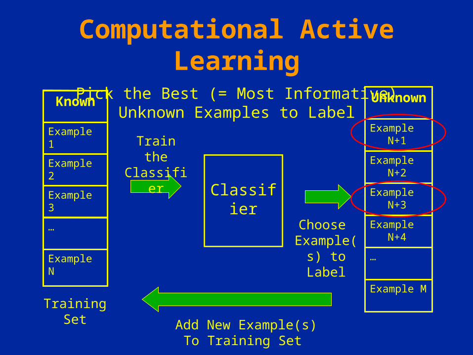
Example M

…

Example N+4

Example N+3

Example N+2

Example N+1

Unknown

Example N

…

Example 3

Example 2

Example 1

Known

Training Set

Classifier

Train the Classifier

Add New Example(s)To Training Set

Choose Example(s)

to Label

Computational Active LearningPick the Best (= Most Informative) Unknown Examples

to Label

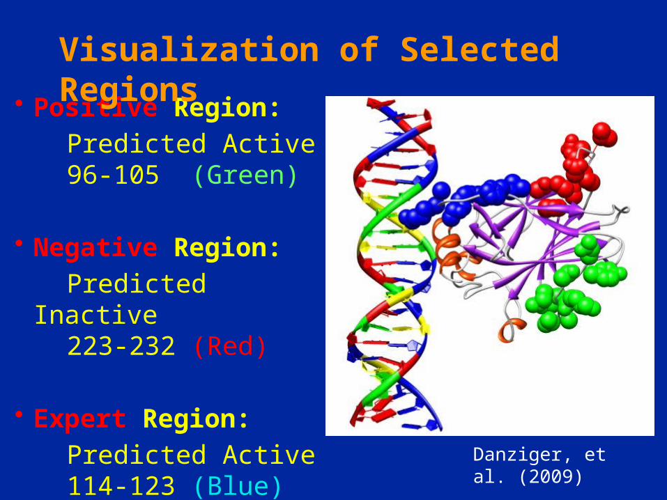
• Positive Region:

Predicted Active96-105  (Green)

• Negative Region:

Predicted Inactive223-232 (Red)

• Expert Region:

Predicted Active114-123 (Blue)

Visualization of Selected Regions

Danziger, et al. (2009)

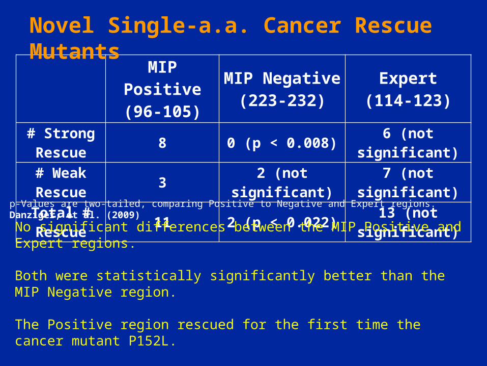
MIP Positive(96-105)

MIP Negative(223-232)

Expert(114-123)

# Strong Rescue 8 0 (p < 0.008) 6 (not significant)

# Weak Rescue 3 2 (not significant) 7 (not significant)

Total # Rescue 11 2 (p < 0.022) 13 (not significant)

p-Values are two-tailed, comparing Positive to Negative and Expert regions. Danziger, et al. (2009)

Novel Single-a.a. Cancer Rescue Mutants

No significant differences between the MIP Positive and Expert regions.

Both were statistically significantly better than the MIP Negative region.

The Positive region rescued for the first time the cancer mutant P152L.

No previous single-a.a. rescue mutants in any region.

Complete architectures for intelligence?

Search?Solve the problem of what to do.

Learning?Learn what to do.

Logic and inference?Reason about what to do.Encoded knowledge/”expert” systems?

Know what to do.

Modern view: It’s complex & multi-faceted.

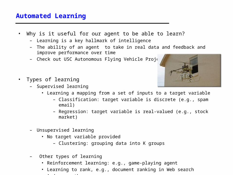
Automated Learning

• Why is it useful for our agent to be able to learn?– Learning is a key hallmark of intelligence– The ability of an agent to take in real data and feedback and improve

performance over time– Check out USC Autonomous Flying Vehicle Project!

• Types of learning– Supervised learning

• Learning a mapping from a set of inputs to a target variable– Classification: target variable is discrete (e.g., spam email)– Regression: target variable is real-valued (e.g., stock market)

– Unsupervised learning• No target variable provided

– Clustering: grouping data into K groups

– Other types of learning• Reinforcement learning: e.g., game-playing agent• Learning to rank, e.g., document ranking in Web search• And many others….

The importance of a good representation

• Properties of a good representation:

• Reveals important features • Hides irrelevant detail• Exposes useful constraints• Makes frequent operations easy-to-do• Supports local inferences from local features

• Called the “soda straw” principle or “locality” principle• Inference from features “through a soda straw”

• Rapidly or efficiently computable• It’s nice to be fast

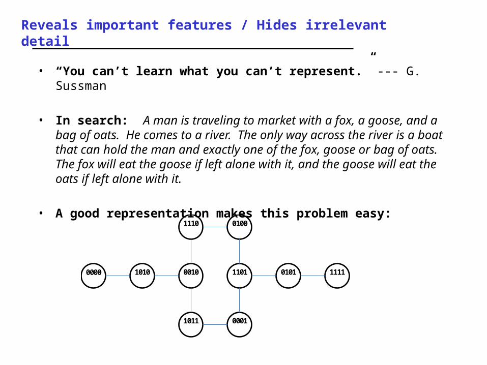
Reveals important features / Hides irrelevant detail

• “You can’t learn what you can’t represent.” --- G. Sussman

• In search: A man is traveling to market with a fox, a goose, and a bag of oats. He comes to a river. The only way across the river is a boat that can hold the man and exactly one of the fox, goose or bag of oats. The fox will eat the goose if left alone with it, and the goose will eat the oats if left alone with it.

• A good representation makes this problem easy:

111000101010111100010101

0000 1101

1011

0100 1110

0010 1010 1111

0001

0101

Simple illustrative learning problem

Problem: decide whether to wait for a table at a restaurant, based on the following attributes:

1. Alternate: is there an alternative restaurant nearby?2. Bar: is there a comfortable bar area to wait in?3. Fri/Sat: is today Friday or Saturday?4. Hungry: are we hungry?5. Patrons: number of people in the restaurant (None, Some, Full)6. Price: price range ($, $$, $$$)7. Raining: is it raining outside?8. Reservation: have we made a reservation?9. Type: kind of restaurant (French, Italian, Thai, Burger)10. WaitEstimate: estimated waiting time (0-10, 10-30, 30-60, >60)

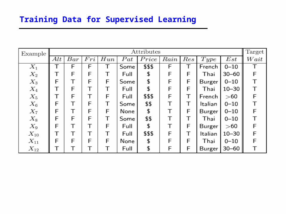
Training Data for Supervised Learning

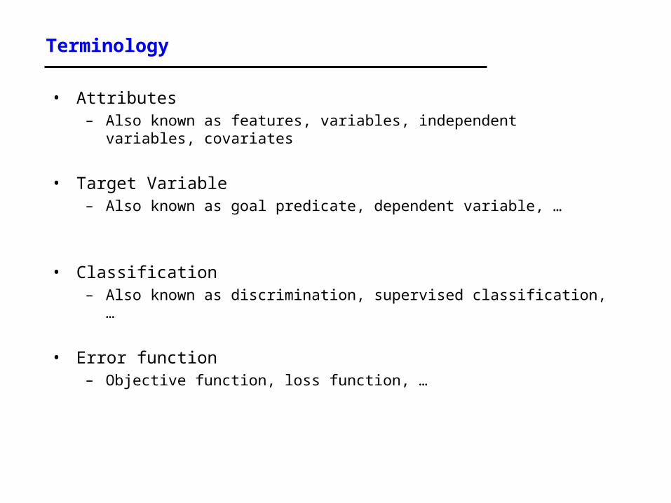
Terminology

• Attributes– Also known as features, variables, independent variables,

covariates

• Target Variable– Also known as goal predicate, dependent variable, …

• Classification– Also known as discrimination, supervised classification, …

• Error function– Objective function, loss function, …

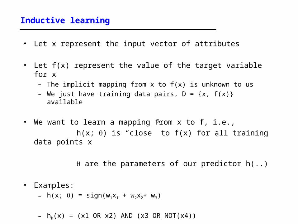
Inductive learning

• Let x represent the input vector of attributes

• Let f(x) represent the value of the target variable for x– The implicit mapping from x to f(x) is unknown to us– We just have training data pairs, D = {x, f(x)} available

• We want to learn a mapping from x to f, i.e., h(x; ) is “close” to f(x) for all training data points x

are the parameters of our predictor h(..)

• Examples:– h(x; ) = sign(w1x1 + w2x2+ w3)

– hk(x) = (x1 OR x2) AND (x3 OR NOT(x4))

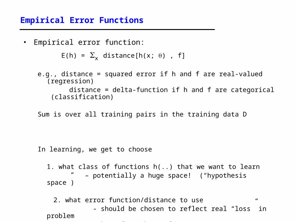
Empirical Error Functions

• Empirical error function:

E(h) = x distance[h(x; ) , f]

e.g., distance = squared error if h and f are real-valued (regression) distance = delta-function if h and f are categorical (classification)

Sum is over all training pairs in the training data D

In learning, we get to choose

1. what class of functions h(..) that we want to learn – potentially a huge space! (“hypothesis space”)

2. what error function/distance to use - should be chosen to reflect real “loss” in problem - but often chosen for mathematical/algorithmic convenience

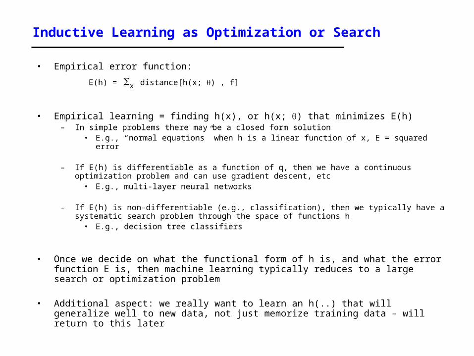
Inductive Learning as Optimization or Search

• Empirical error function:

E(h) = x distance[h(x; ) , f]

• Empirical learning = finding h(x), or h(x; ) that minimizes E(h)– In simple problems there may be a closed form solution

• E.g., “normal equations” when h is a linear function of x, E = squared error

– If E(h) is differentiable as a function of q, then we have a continuous optimization problem and can use gradient descent, etc

• E.g., multi-layer neural networks

– If E(h) is non-differentiable (e.g., classification), then we typically have a systematic search problem through the space of functions h

• E.g., decision tree classifiers

• Once we decide on what the functional form of h is, and what the error function E is, then machine learning typically reduces to a large search or optimization problem

• Additional aspect: we really want to learn an h(..) that will generalize well to new data, not just memorize training data – will return to this later

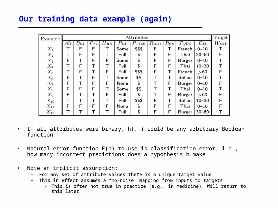
Our training data example (again)

• If all attributes were binary, h(..) could be any arbitrary Boolean function

• Natural error function E(h) to use is classification error, i.e., how many incorrect predictions does a hypothesis h make

• Note an implicit assumption:– For any set of attribute values there is a unique target value– This in effect assumes a “no-noise” mapping from inputs to targets

• This is often not true in practice (e.g., in medicine). Will return to this later

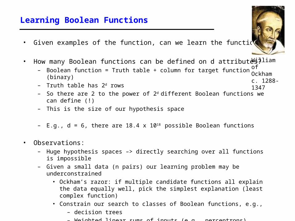
Learning Boolean Functions

• Given examples of the function, can we learn the function?

• How many Boolean functions can be defined on d attributes?– Boolean function = Truth table + column for target function (binary)– Truth table has 2d rows– So there are 2 to the power of 2d different Boolean functions we can define

(!)– This is the size of our hypothesis space

– E.g., d = 6, there are 18.4 x 1018 possible Boolean functions

• Observations:– Huge hypothesis spaces –> directly searching over all functions is impossible– Given a small data (n pairs) our learning problem may be underconstrained

• Ockham’s razor: if multiple candidate functions all explain the data equally well, pick the simplest explanation (least complex function)

• Constrain our search to classes of Boolean functions, e.g.,– decision trees– Weighted linear sums of inputs (e.g., perceptrons)

William ofOckhamc. 1288-1347

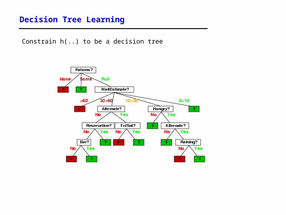
Decision Tree Learning

Constrain h(..) to be a decision tree

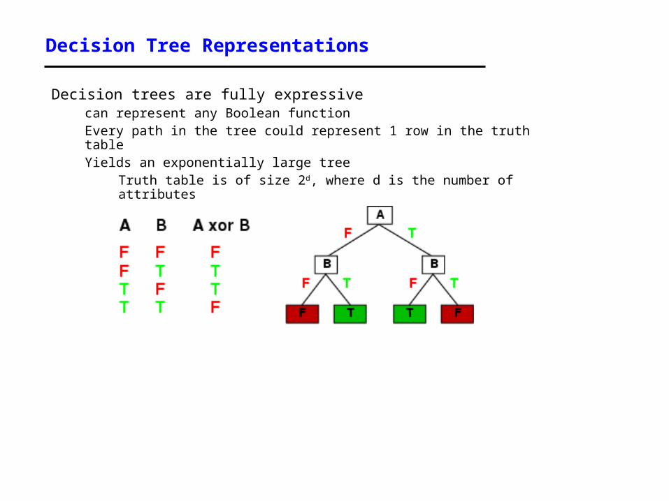
Decision Tree Representations

Decision trees are fully expressivecan represent any Boolean functionEvery path in the tree could represent 1 row in the truth tableYields an exponentially large tree

Truth table is of size 2d, where d is the number of attributes

Decision Tree Representations

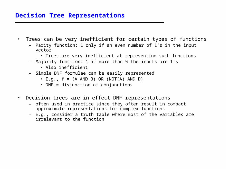
• Trees can be very inefficient for certain types of functions– Parity function: 1 only if an even number of 1’s in the input vector

• Trees are very inefficient at representing such functions– Majority function: 1 if more than ½ the inputs are 1’s

• Also inefficient– Simple DNF formulae can be easily represented

• E.g., f = (A AND B) OR (NOT(A) AND D)• DNF = disjunction of conjunctions

• Decision trees are in effect DNF representations– often used in practice since they often result in compact approximate

representations for complex functions– E.g., consider a truth table where most of the variables are irrelevant to the

function

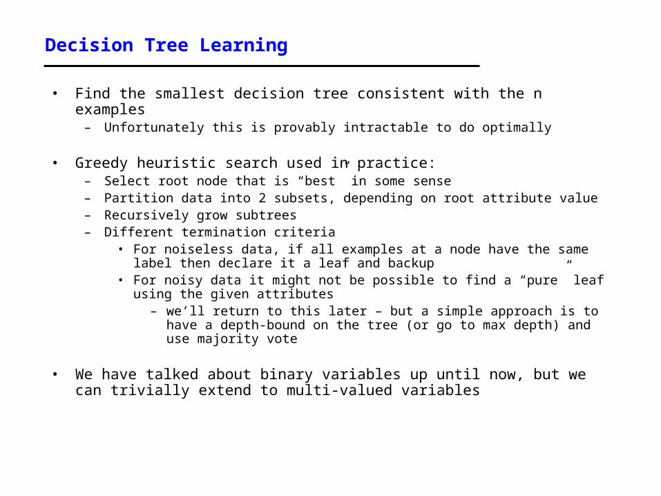
Decision Tree Learning

• Find the smallest decision tree consistent with the n examples– Unfortunately this is provably intractable to do optimally

• Greedy heuristic search used in practice:– Select root node that is “best” in some sense– Partition data into 2 subsets, depending on root attribute value– Recursively grow subtrees– Different termination criteria

• For noiseless data, if all examples at a node have the same label then declare it a leaf and backup

• For noisy data it might not be possible to find a “pure” leaf using the given attributes

– we’ll return to this later – but a simple approach is to have a depth-bound on the tree (or go to max depth) and use majority vote

• We have talked about binary variables up until now, but we can trivially extend to multi-valued variables

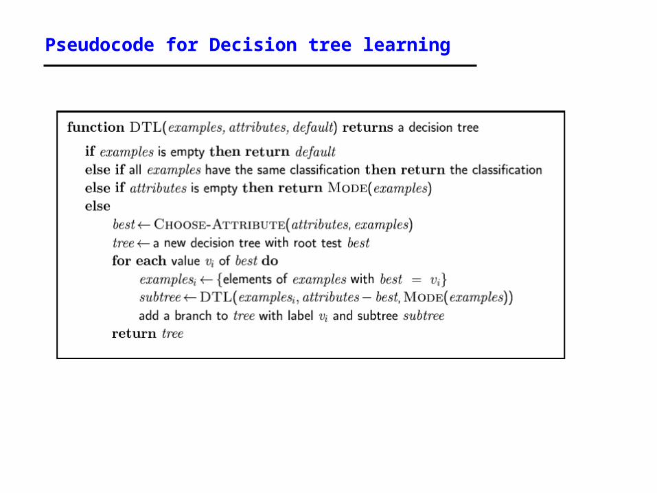
Pseudocode for Decision tree learning

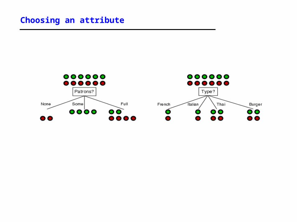
Choosing an attribute

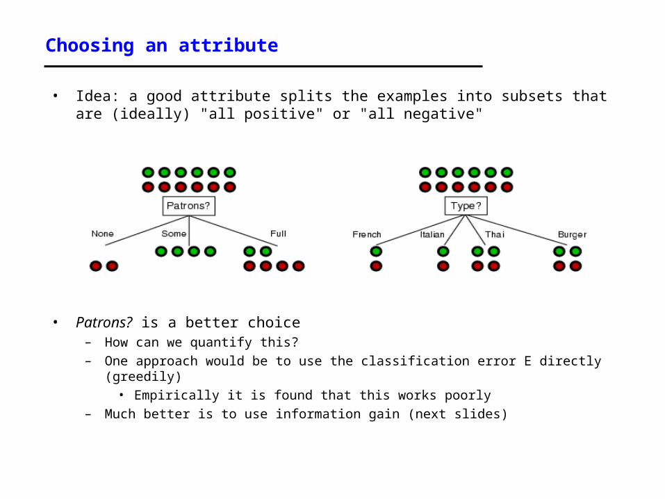
• Idea: a good attribute splits the examples into subsets that are (ideally) "all positive" or "all negative"

• Patrons? is a better choice– How can we quantify this?– One approach would be to use the classification error E directly (greedily)

• Empirically it is found that this works poorly– Much better is to use information gain (next slides)

Entropy

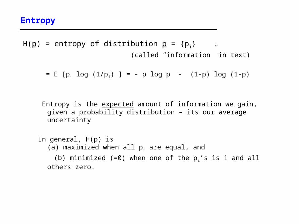
H(p) = entropy of distribution p = {pi}

(called “information” in text)

= E [pi log (1/pi) ] = - p log p - (1-p) log (1-p)

Entropy is the expected amount of information we gain, given a probability distribution – its our average uncertainty

In general, H(p) is(a) maximized when all pi are equal, and

(b) minimized (=0) when one of the pi’s is 1 and all others zero.

Entropy with only 2 outcomes

Consider 2 class problem: p = probability of class 1, 1 – p = probability of class 2

In binary case, H(p) = - p log p - (1-p) log (1-p)

H(p)

0.5 10

1

p

Information Gain

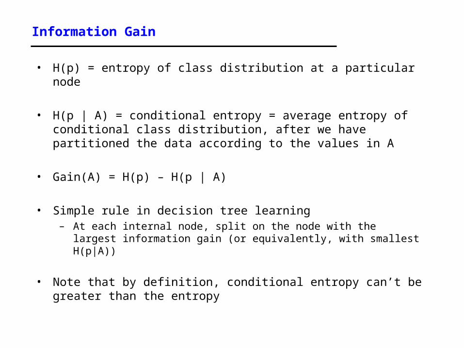
• H(p) = entropy of class distribution at a particular node

• H(p | A) = conditional entropy = average entropy of conditional class distribution, after we have partitioned the data according to the values in A

• Gain(A) = H(p) – H(p | A)

• Simple rule in decision tree learning– At each internal node, split on the node with the largest information

gain (or equivalently, with smallest H(p|A))

• Note that by definition, conditional entropy can’t be greater than the entropy

Root Node Example

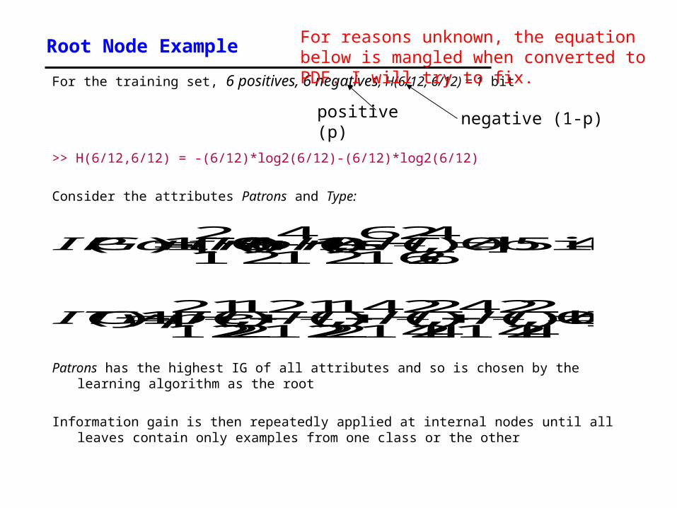
For the training set, 6 positives, 6 negatives, H(6/12, 6/12) = 1 bit

>> H(6/12,6/12) = -(6/12)*log2(6/12)-(6/12)*log2(6/12)

Consider the attributes Patrons and Type:

Patrons has the highest IG of all attributes and so is chosen by the learning algorithm as the root

Information gain is then repeatedly applied at internal nodes until all leaves contain only examples from one class or the other

b its 0)]4

2,

4

2(

1 2

4)

4

2,

4

2(

1 2

4)

2

1,

2

1(

1 2

2)

2

1,

2

1(

1 2

2[1)(

b its 0 5 4 1.)]6

4,

6

2(

1 2

6)0,1(

1 2

4)1,0(

1 2

2[1)(

HHHHTyp eIG

HHHPa tro n sIG

positive (p) negative (1-p)

For reasons unknown, the equation below is mangled when converted to PDF. I will try to fix.

Choosing an attribute

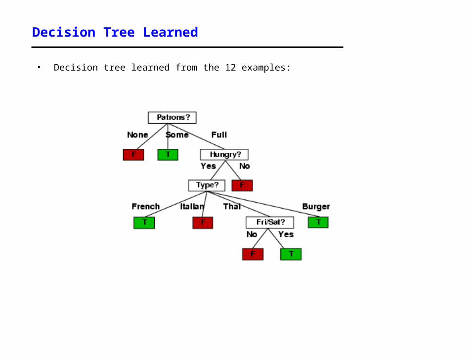
Decision Tree Learned

• Decision tree learned from the 12 examples:

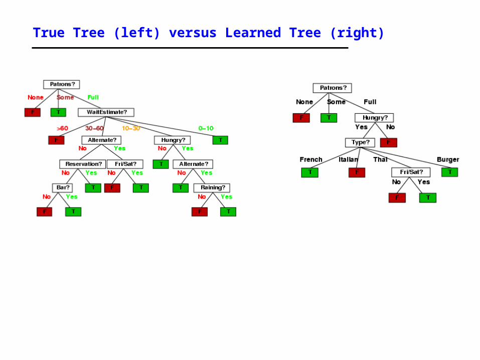
True Tree (left) versus Learned Tree (right)

Assessing Performance

Training data performance is typically optimistice.g., error rate on training data

Reasons?- classifier may not have enough data to fully learn the concept (but

on training data we don’t know this) - for noisy data, the classifier may overfit the training data

In practice we want to assess performance “out of sample”how well will the classifier do on new unseen data? This is the

true test of what we have learned (just like a classroom)

With large data sets we can partition our data into 2 subsets, train and test- build a model on the training data

- assess performance on the test data

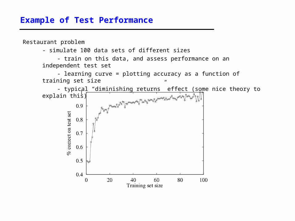
Example of Test Performance

Restaurant problem- simulate 100 data sets of different sizes

- train on this data, and assess performance on an independent test set - learning curve = plotting accuracy as a function of training set size - typical “diminishing returns” effect (some nice theory to explain this)

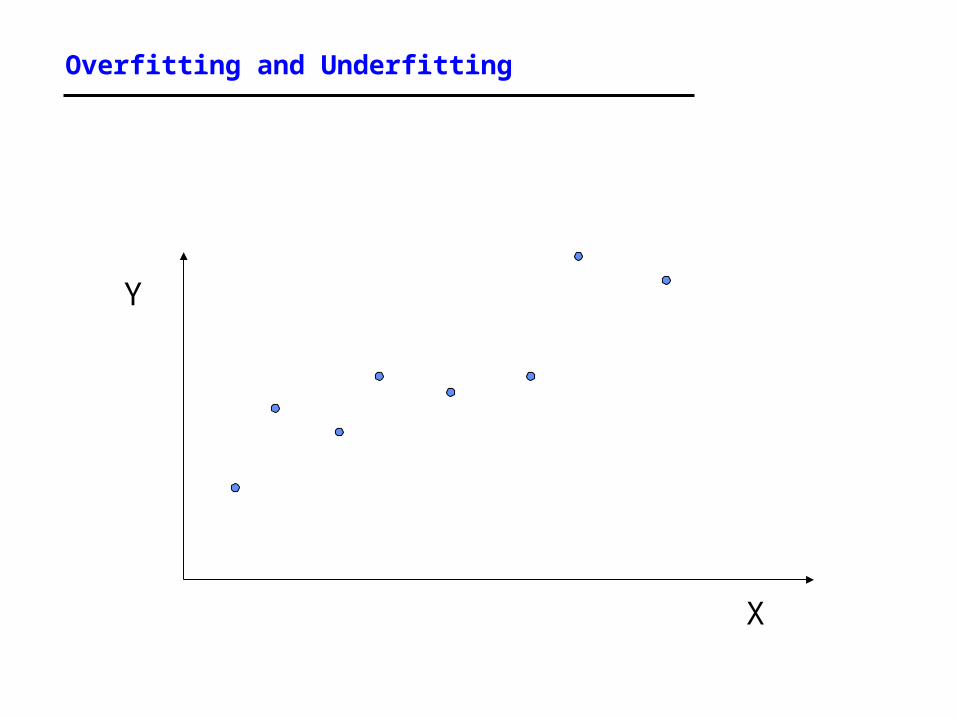
Overfitting and Underfitting

X

Y

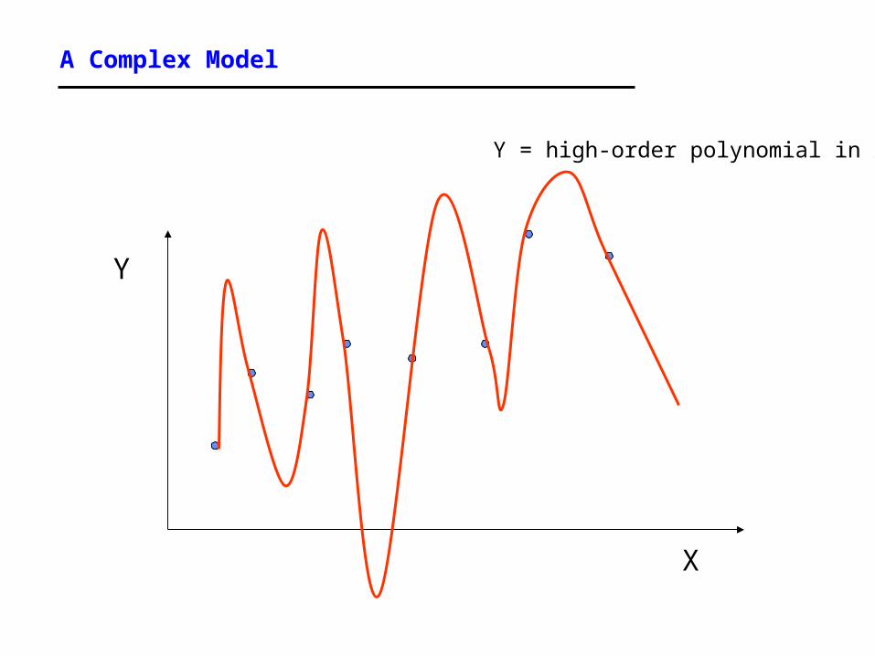
A Complex Model

X

Y

Y = high-order polynomial in X

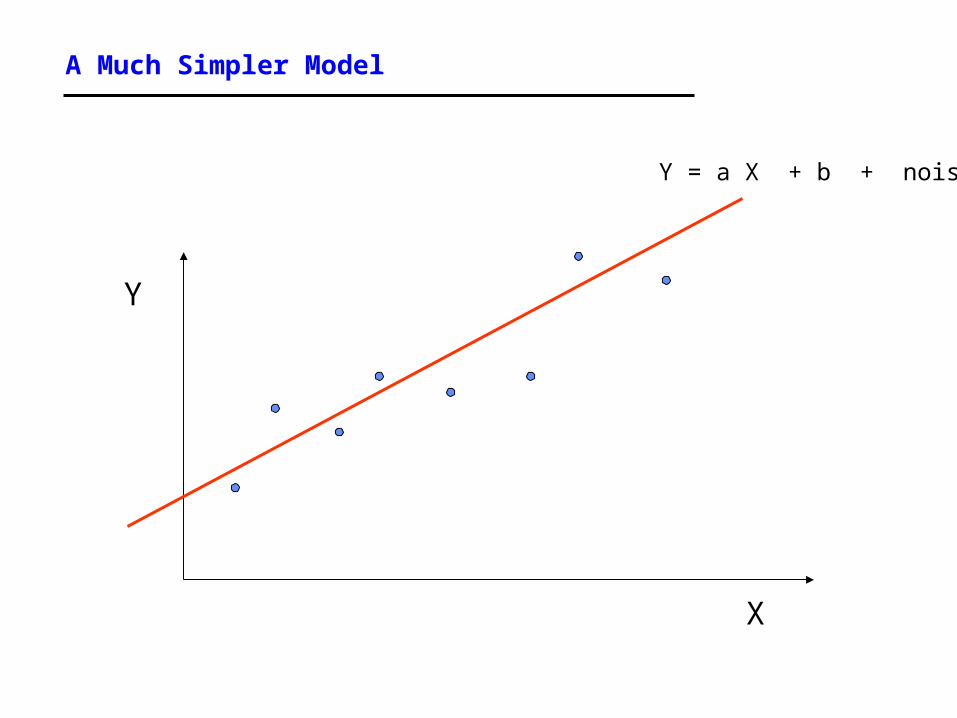
A Much Simpler Model

X

Y

Y = a X + b + noise

Example 2

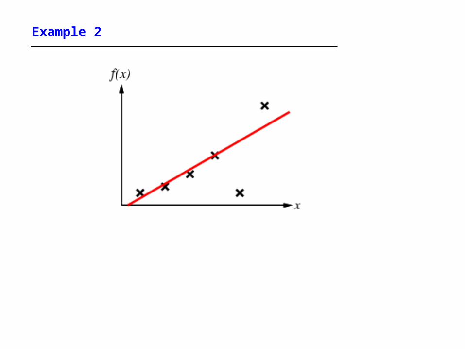
Example 2

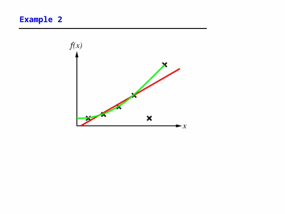
Example 2

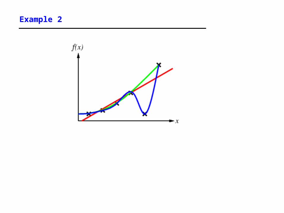
Example 2

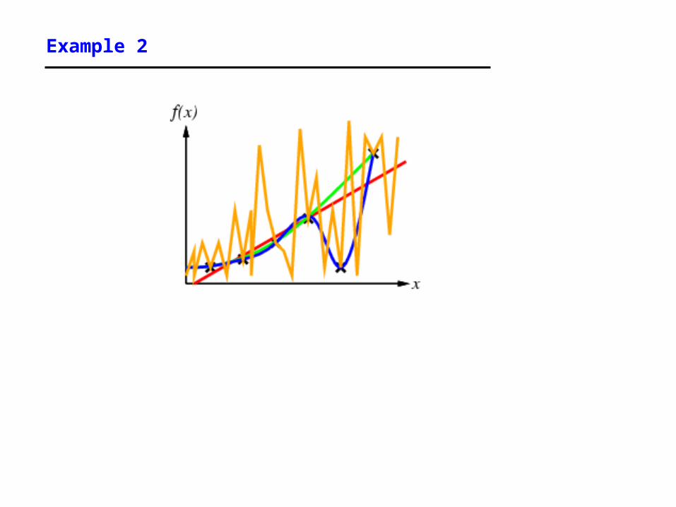
Example 2

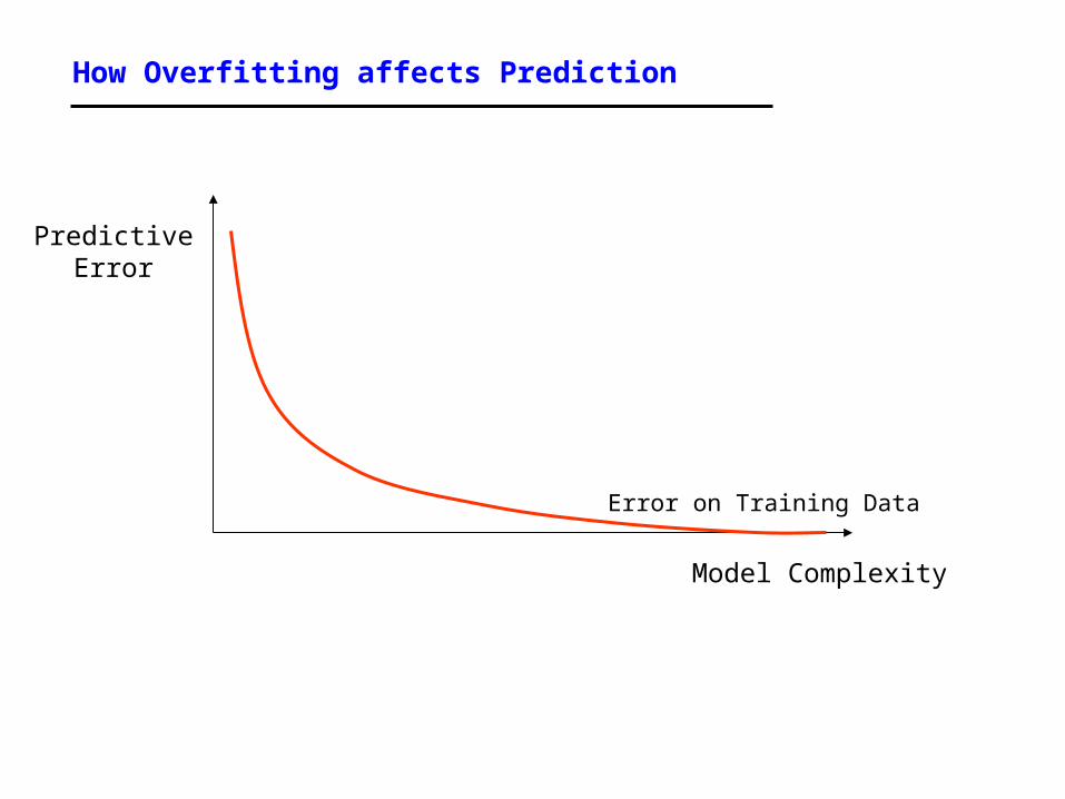
How Overfitting affects Prediction

PredictiveError

Model Complexity

Error on Training Data

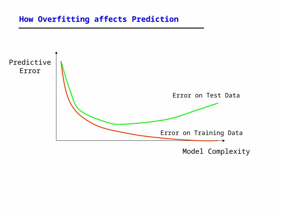
How Overfitting affects Prediction

PredictiveError

Model Complexity

Error on Training Data

Error on Test Data

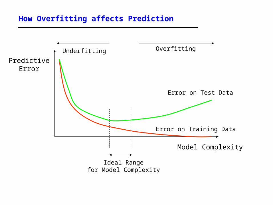
How Overfitting affects Prediction

PredictiveError

Model Complexity

Error on Training Data

Error on Test Data

Ideal Rangefor Model Complexity

OverfittingUnderfitting

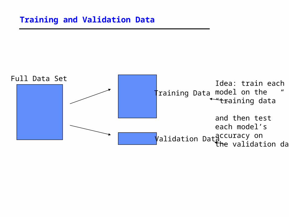
Training and Validation Data

Full Data Set

Training Data

Validation Data

Idea: train eachmodel on the“training data”

and then testeach model’saccuracy onthe validation data

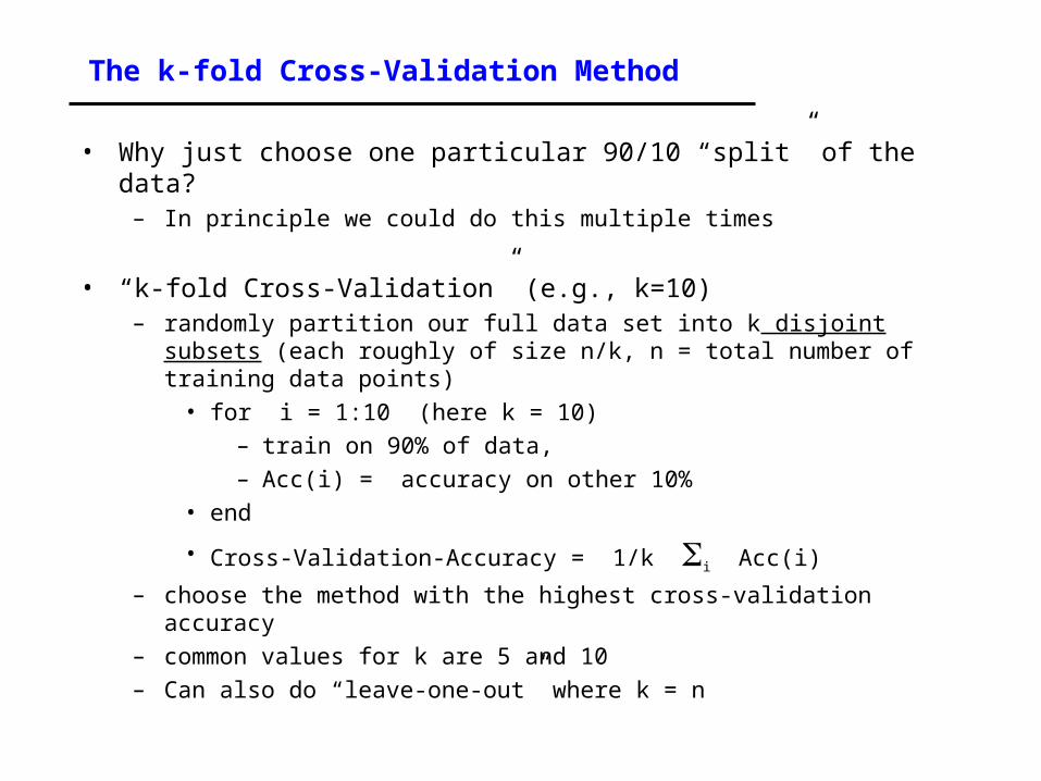
The k-fold Cross-Validation Method

• Why just choose one particular 90/10 “split” of the data?– In principle we could do this multiple times

• “k-fold Cross-Validation” (e.g., k=10)– randomly partition our full data set into k disjoint subsets (each

roughly of size n/k, n = total number of training data points)• for i = 1:10 (here k = 10)

– train on 90% of data,– Acc(i) = accuracy on other 10%

• end

• Cross-Validation-Accuracy = 1/k i Acc(i)

– choose the method with the highest cross-validation accuracy– common values for k are 5 and 10– Can also do “leave-one-out” where k = n

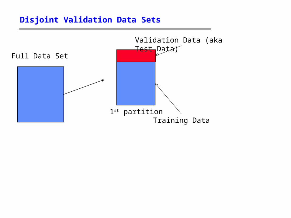
Disjoint Validation Data Sets

Full Data Set

Training Data

Validation Data (aka Test Data)

1st partition

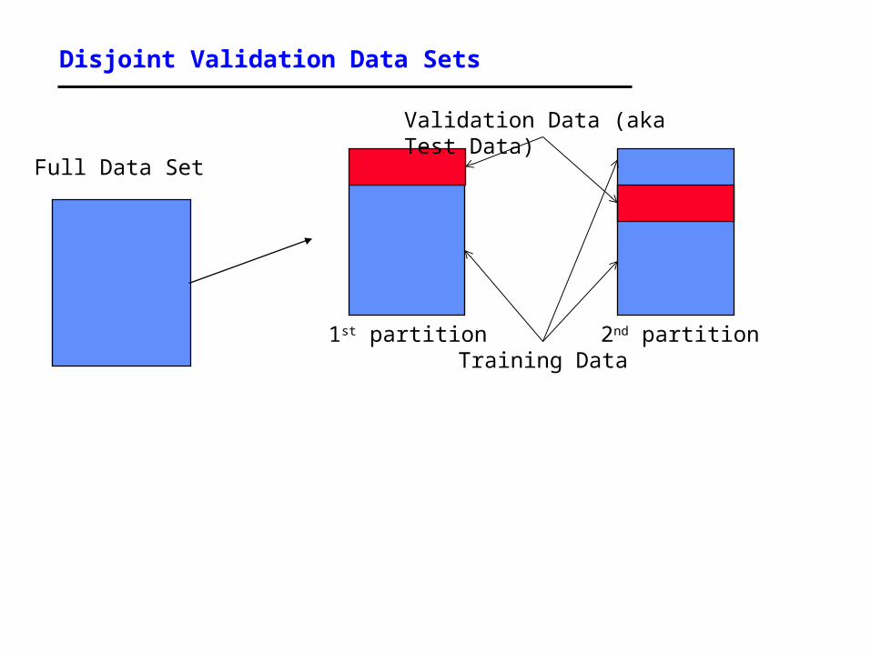
Disjoint Validation Data Sets

Full Data Set

Training Data

Validation Data (aka Test Data)

1st partition 2nd partition

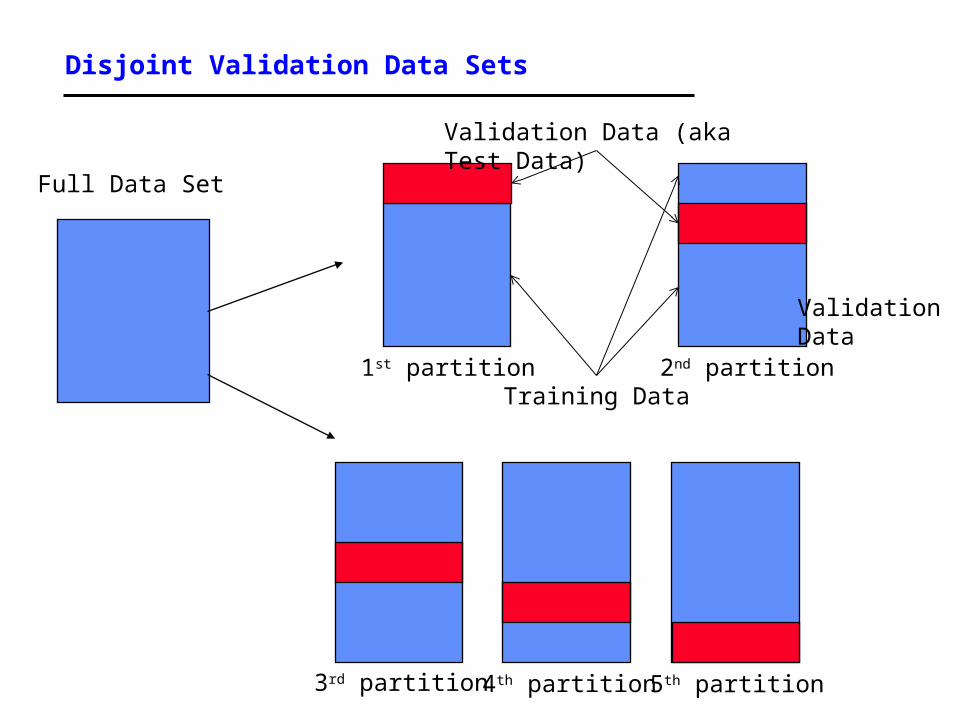
Disjoint Validation Data Sets

Full Data Set

Training Data

Validation Data (aka Test Data)

Validation Data

1st partition 2nd partition

3rd partition 4th partition 5th partition

More on Cross-Validation

• Notes– cross-validation generates an approximate estimate of how well the

learned model will do on “unseen” data

– by averaging over different partitions it is more robust than just a single train/validate partition of the data

– “k-fold” cross-validation is a generalization• partition data into disjoint validation subsets of size n/k• train, validate, and average over the v partitions• e.g., k=10 is commonly used

– k-fold cross-validation is approximately k times computationally more expensive than just fitting a model to all of the data

Summary

• Inductive learning– Error function, class of hypothesis/models {h}– Want to minimize E on our training data– Example: decision tree learning

• Generalization– Training data error is over-optimistic– We want to see performance on test data– Cross-validation is a useful practical approach

• Learning to recognize faces– Viola-Jones algorithm: state-of-the-art face detector, entirely

learned from data, using boosting+decision-stumps