INTRODUCTION

TO

MACHINE

LEARNING 3RD EDITION

ETHEM ALPAYDIN

© The MIT Press, 2014

alpaydin@boun.edu.tr

http://www.cmpe.boun.edu.tr/~ethem/i2ml3e

Lecture Slides for

CHAPTER 11:

MULTILAYER PERCEPTRONS

Neural Networks 3

Networks of processing units (neurons) with

connections (synapses) between them

Large number of neurons: 1010

Large connectitivity: 105

Parallel processing

Distributed computation/memory

Robust to noise, failures

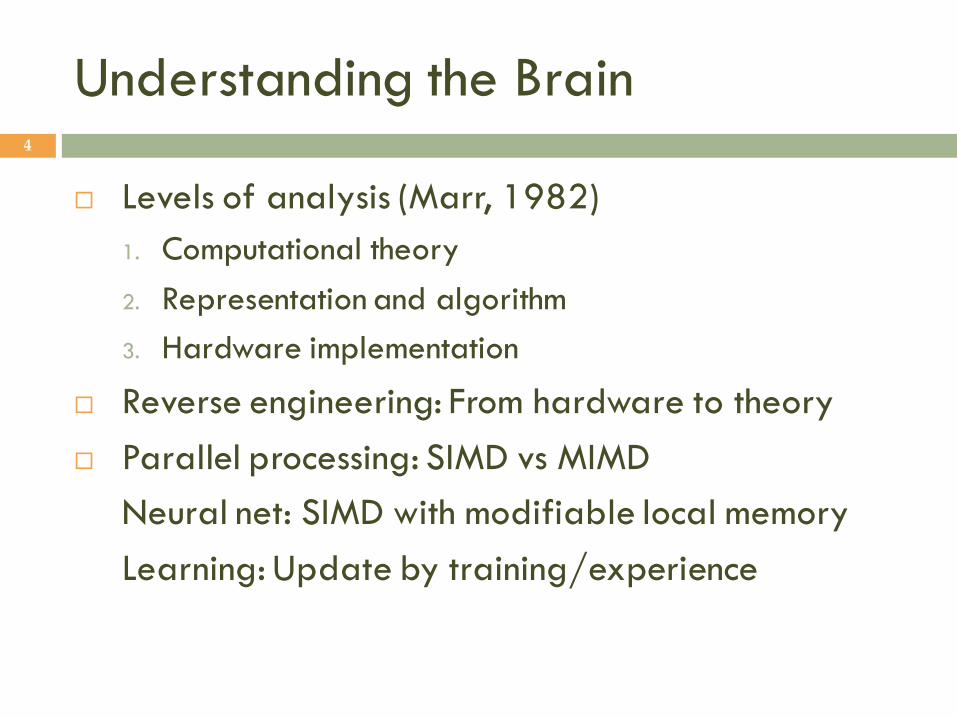
Understanding the Brain 4

Levels of analysis (Marr, 1982)

1. Computational theory

2. Representation and algorithm

3. Hardware implementation

Reverse engineering: From hardware to theory

Parallel processing: SIMD vs MIMD

Neural net: SIMD with modifiable local memory

Learning: Update by training/experience

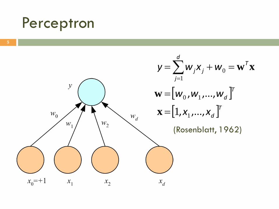
Perceptron 5

Td

T

d

Td

jjj

xx

www

wxwy

,...,,

,...,,

1

10

0

1

1

x

w

xw

(Rosenblatt, 1962)

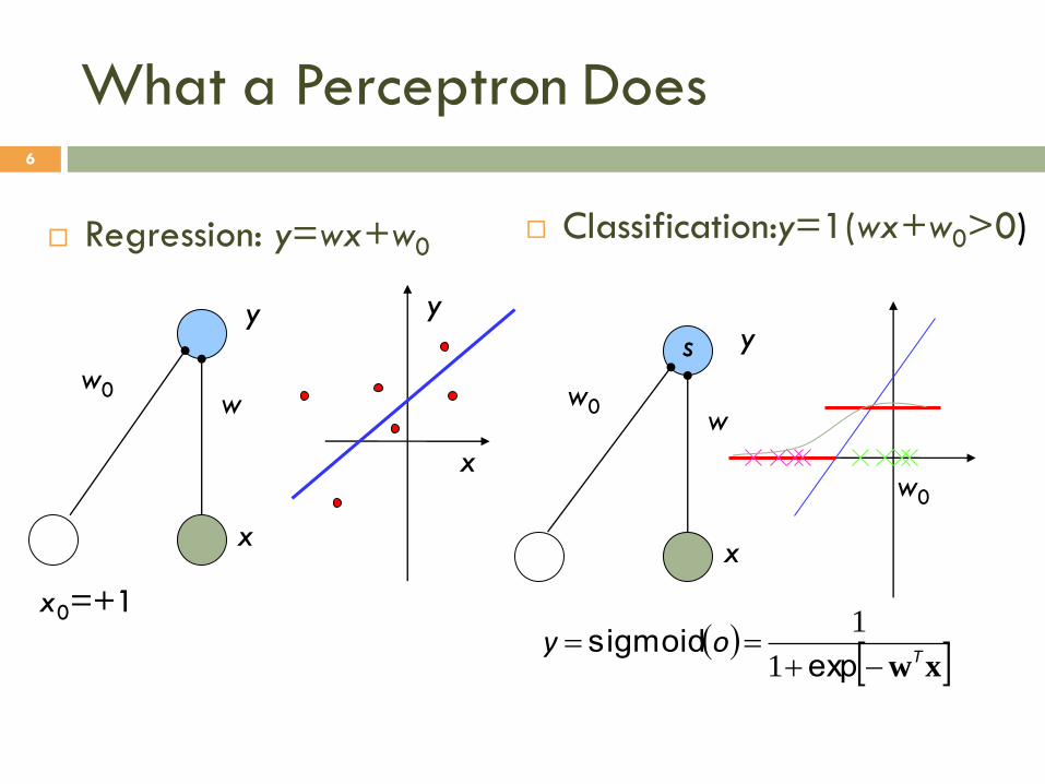
What a Perceptron Does

Regression: y=wx+w0 Classification:y=1(wx+w0>0)

6

w w0

y

x

x0=+1

w w0

y

x

s

w0

y

x

xw

Toy

exp sigmoid

1

1

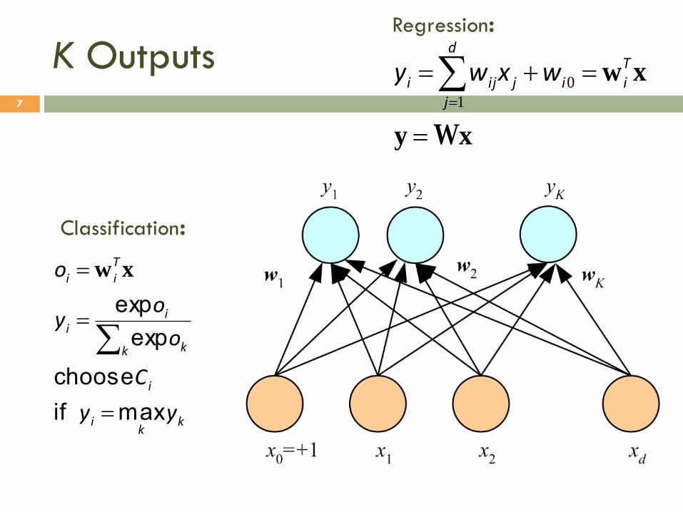
K Outputs 7

kk

i

i

k k

ii

Tii

yy

C

o

oy

o

max if

choose

exp

exp

xw

xy

xw

W

Tii

d

jjiji wxwy 0

1

Classification:

Regression:

Online (instances seen one by one) vs batch (whole sample) learning:

No need to store the whole sample

Problem may change in time

Wear and degradation in system components

Stochastic gradient-descent: Update after a single pattern

Generic update rule (LMS rule):

Training 8

InpututActualOutpputDesiredOutctorLearningFaUpdate

tj

ti

ti

tij xyrw

Training a Perceptron: Regression

Regression (Linear output):

tj

tttj

tTtttttt

xyrw

ryrrE

22

2

1

2

1xwxw ,|

9

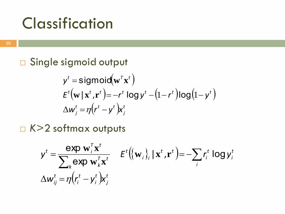
Single sigmoid output

K>2 softmax outputs

Classification 10

tj

tttj

ttttttt

tTt

xyrw

yryrE

y

11 log log |

sigmoid

rxw

xw

,

tj

ti

ti

tij

i

ti

ti

tt

iit

k

tTk

tTit

xyrw

yrEy

log | exp

exprxw

xw

xw,

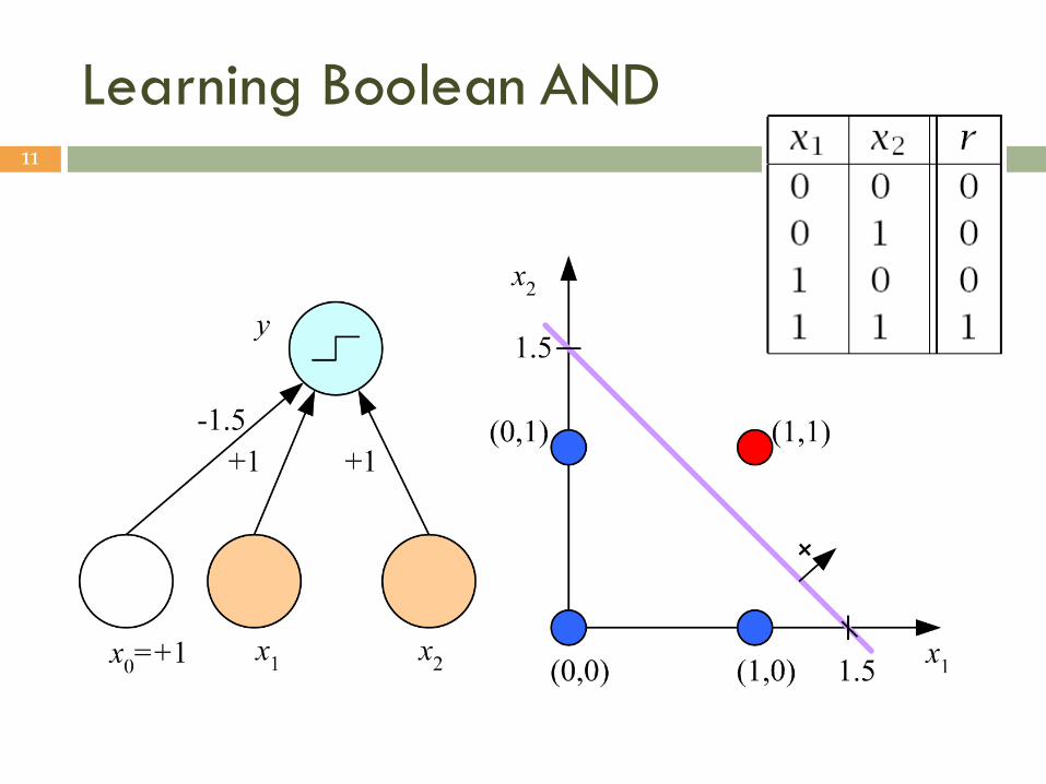
Learning Boolean AND 11

XOR

No w0, w1, w2 satisfy:

0

0

0

0

021

01

02

0

www

ww

ww

w

12

(Minsky and Papert, 1969)

Multilayer Perceptrons 13

d

j hjhj

Thh

H

hihih

Tii

wxw

z

vzvy

1 0

1

0

1

1

exp

sigmoid xw

zv

(Rumelhart et al., 1986)

14 x1 XOR x2 = (x1 AND ~x2) OR (~x1 AND x2)

Backpropagation 15

hj

h

h

i

ihj

d

j hjhj

Thh

H

hihih

Tii

w

z

z

y

y

E

w

E

wxw

z

vzvy

exp

sigmoid

1 0

1

0

1

1

xw

zv

16

xwThhz sigmoid

H

h

thh

t vzvy1

0

tj

th

th

th

tt

tj

th

th

th

tt

hj

th

th

t

tt

hj

hj

xzzvyr

xzzvyr

w

z

z

y

y

E

w

Ew

1

1

Regression

Forward

Backward

x

22

1 t

tt yrE X|,vW

th

t

tth zyrv

Regression with Multiple Outputs 17

tj

th

th

t iih

ti

tihj

th

t

ti

tiih

i

H

h

thih

ti

t i

ti

ti

xzzvyrw

zyrv

vzvy

yrE

1

2

1

0

1

2

X|,VW

zh

vih

yi

xj

whj

18

19

20

whx+w0

zh vhzh

One sigmoid output yt for P(C1|xt) and

P(C2|xt) ≡ 1-yt

Two-Class Discrimination 21

tj

th

thh

t

tthj

th

t

tth

t

tttt

H

h

thh

t

xzzvyrw

zyrv

yryrE

vzvy

1

11

1

0

log log |

sigmoid

Xv,W

K>2 Classes 22

tj

th

th

t iih

ti

tihj

th

t

ti

tiih

t i

ti

ti

ti

k

tk

tit

i

H

hi

thih

ti

xzzvyrw

zyrv

yrE

CPo

oyvzvo

1

1

0

log|

| exp

exp

Xv

x

,W

Multiple Hidden Layers 23

2

1

1

022

2

1

0212122

1

1

01111

1

1

H

lll

T

H

hlhlh

Tll

d

jhjhj

Thh

vzvy

Hlwzwz

Hhwxwz

zv

zw

xw

,...,,

,...,,

sigmoid sigmoid

sigmoid sigmoid

MLP with one hidden layer is a universal

approximator (Hornik et al., 1989), but using

multiple layers may lead to simpler networks

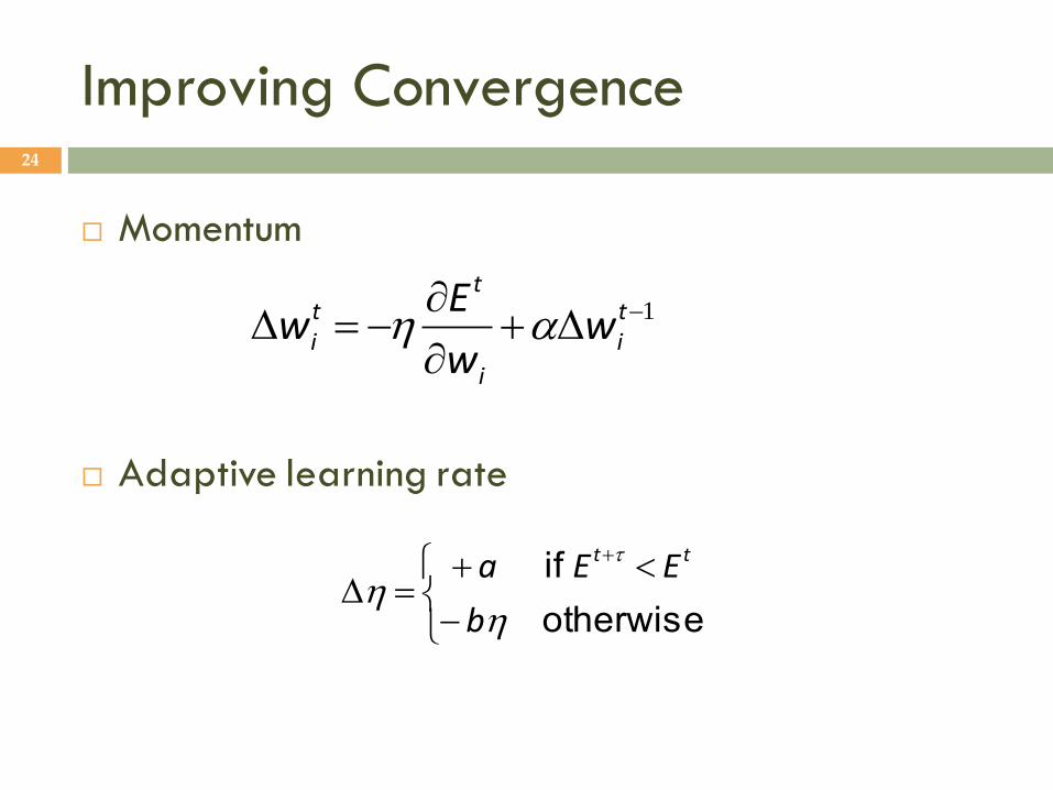
Momentum

Adaptive learning rate

Improving Convergence 24

1

t

i

i

tti w

w

Ew

otherwise

if

b

EEa tt

Overfitting/Overtraining 25

Number of weights: H (d+1)+(H+1)K

26

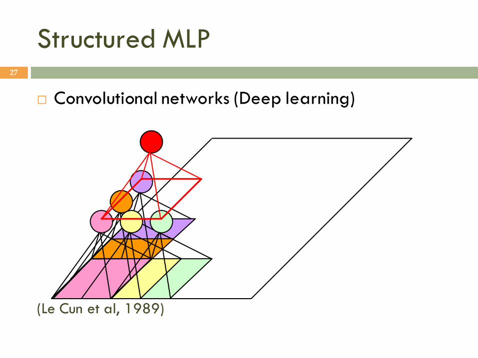
Structured MLP 27

Convolutional networks (Deep learning)

(Le Cun et al, 1989)

Weight Sharing 28

Hints 29

xx

xx

xx

h

bxgbxg

axgaxg

baxg

E

|i f |

|i f |

,|i f

2

2

0

Invariance to translation, rotation, size

Virtual examples

Augmented error: E’=E+λhEh

If x’ and x are the “same”: Eh=[g(x|θ)- g(x’|θ)]2

Approximation hint:

(Abu-Mostafa, 1995)

Tuning the Network Size

Destructive

Weight decay:

Constructive

Growing networks

30

(Ash, 1989) (Fahlman and Lebiere, 1989)

ii

i

i

i

wEE

ww

Ew

2

2

'

Consider weights wi as random vars, prior p(wi)

Weight decay, ridge regression, regularization

cost=data-misfit + λ complexity

More about Bayesian methods in chapter 14

Bayesian Learning 31

2

2

212

w

w

www

ww

www

w

EE

wcwpwpp

Cppp

pp

ppp

ii

ii

MAP

'

)/(

ˆ

exp where

log| log| log

| log max arg |

|

XX

XX

XX

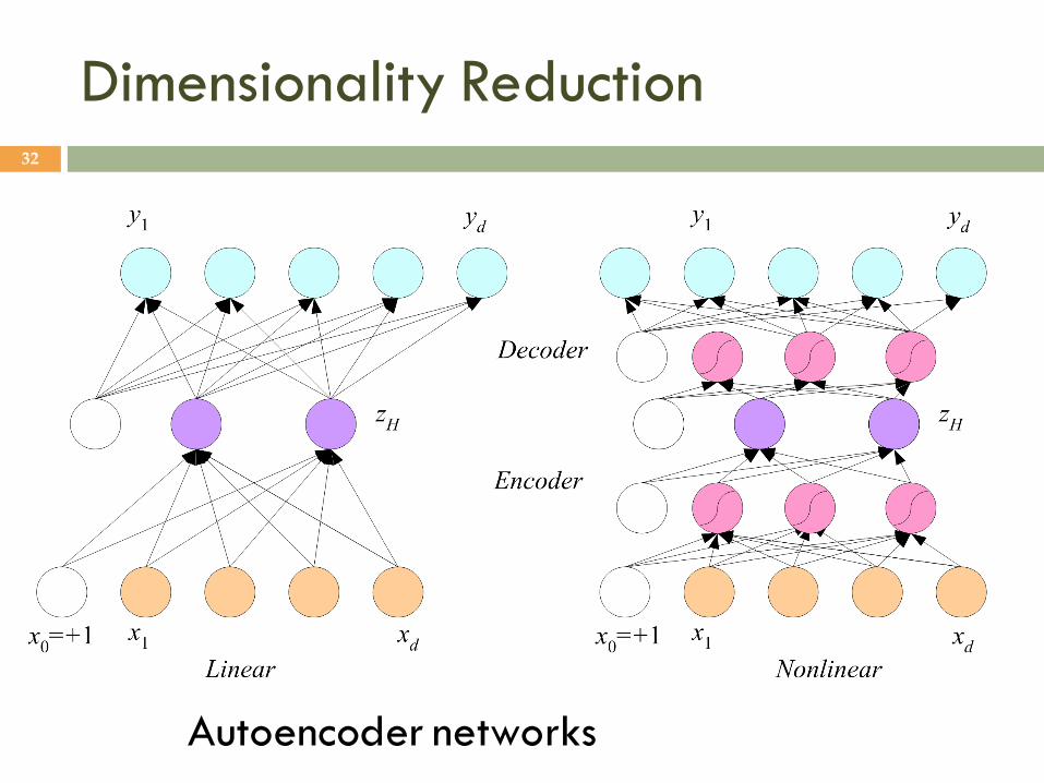
Dimensionality Reduction 32

Autoencoder networks

33

Learning Time 34

Applications:

Sequence recognition: Speech recognition

Sequence reproduction: Time-series prediction

Sequence association

Network architectures

Time-delay networks (Waibel et al., 1989)

Recurrent networks (Rumelhart et al., 1986)

Time-Delay Neural Networks 35

Recurrent Networks 36

Unfolding in Time 37

Deep Networks 38

Layers of feature extraction units

Can have local receptive fields as in convolution

networks, or can be fully connected

Can be trained layer by layer using an autoencoder

in an unsupervised manner

No need to craft the right features or the right basis

functions or the right dimensionality reduction method;

learns multiple layers of abstraction all by itself given

a lot of data and a lot of computation

Applications in vision, language processing, ...