Introduction to Machine Learning

Inas A. Yassine, PhD

Assoc. Prof. , Systems and Biomedical Engineering Department, Cairo University

inas.yassine@eng.cu.edu.eg

Linear regression

• Given an input x we would like to compute an output y

• In linear regression we assume that y and x are related with the following equation:

y = wx + ε where w is a parameter and ε

represents measurement or other noise

2

X

Y

What we are trying to predict

Observed values

Linear regression

3

• Our goal is to estimate w from a training data of <xi,yi> pairs

• Optimization goal: minimize squared error (least squares):

• Why least squares?

- minimizes squared distance between measurements and predicted line

- has a nice probabilistic interpretation

- the math is pretty

∑ −i

iiw wxy 2)(minargX

Y ε+= wxy

Overfitting in Regression

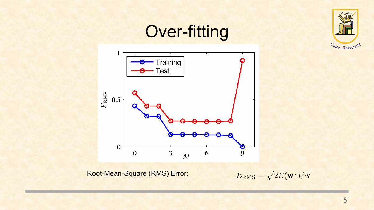
Over-fitting

5

Root-Mean-Square (RMS) Error:

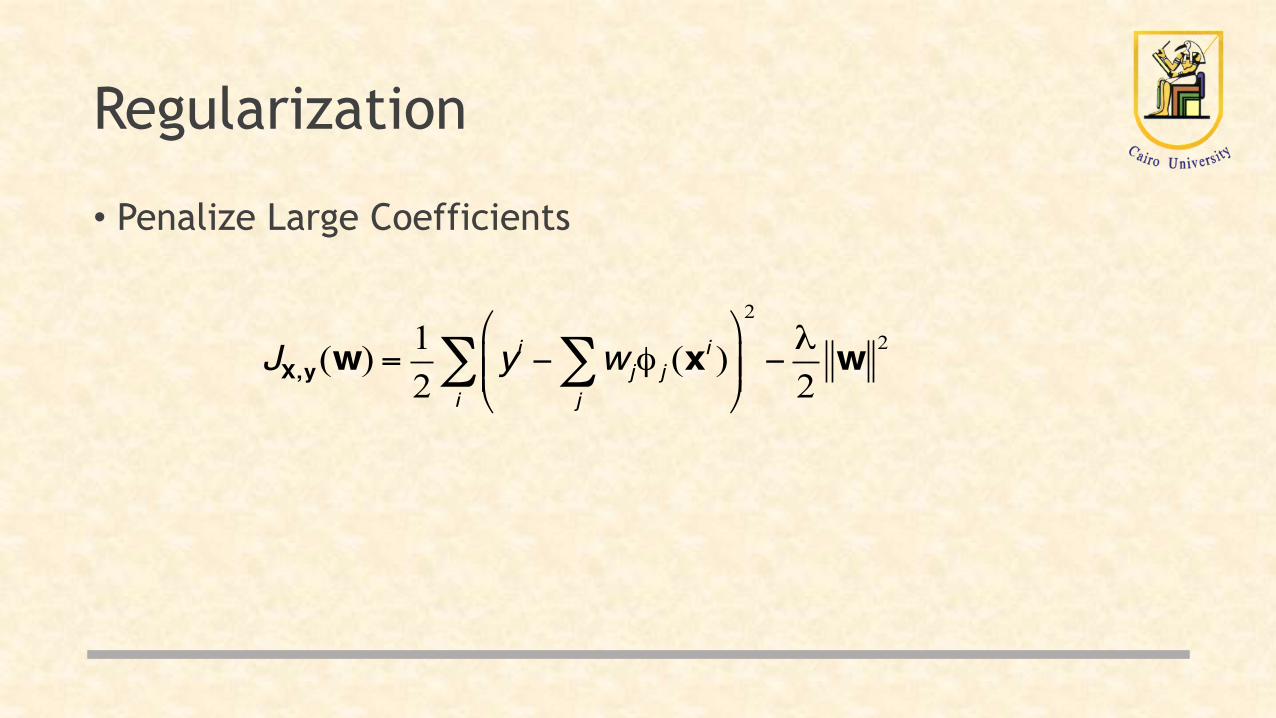
Regularization

• Penalize Large Coefficients

JX,y(w) =12

yi − wjφ j (xi )j∑

⎛

⎝⎜⎜

⎞

⎠⎟⎟

i∑

2

−λ2w 2

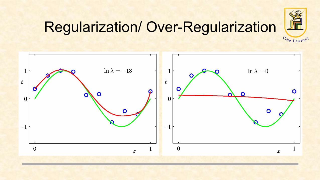
Regularization/ Over-Regularization

Outliers

• Rare/ Extreme values that may destroy the learning, which could be:

• Error • Important observation

• outliers if detected if greater than 3 standard deviation from the mean

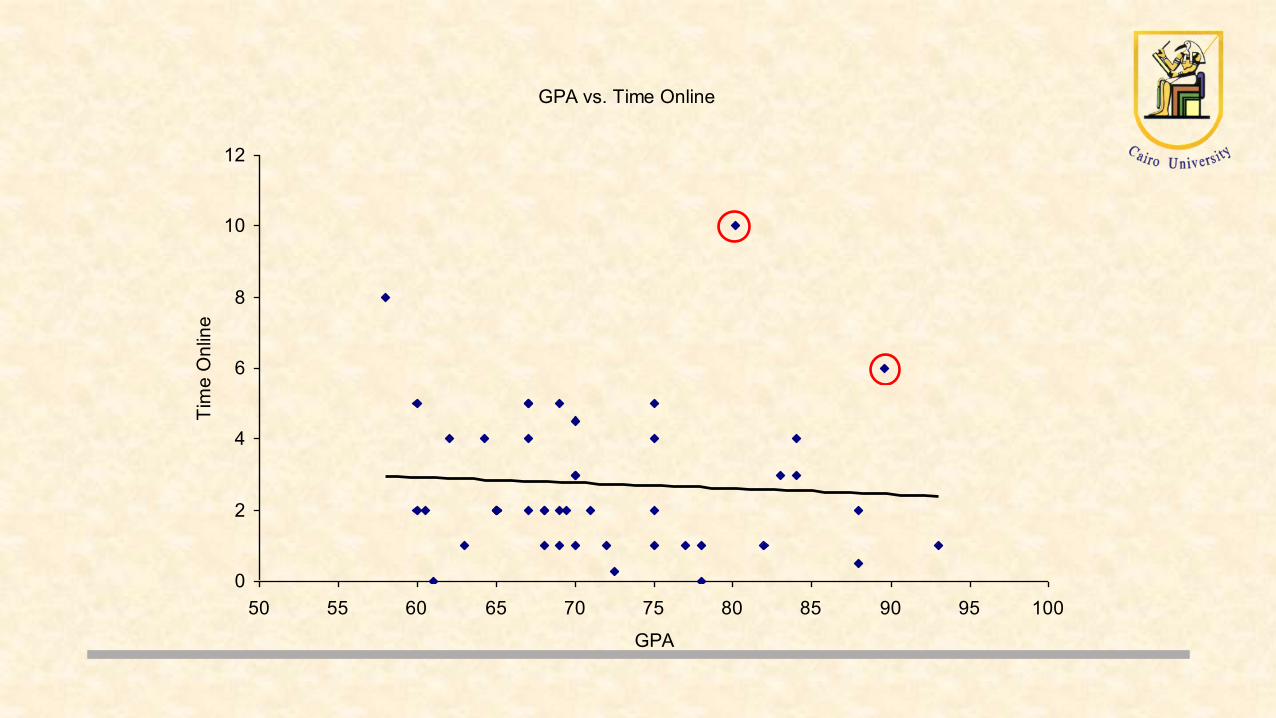
GPA vs. Time Online

0

2

4

6

8

10

12

50 55 60 65 70 75 80 85 90 95 100

GPA

Tim

e O

nlin

e

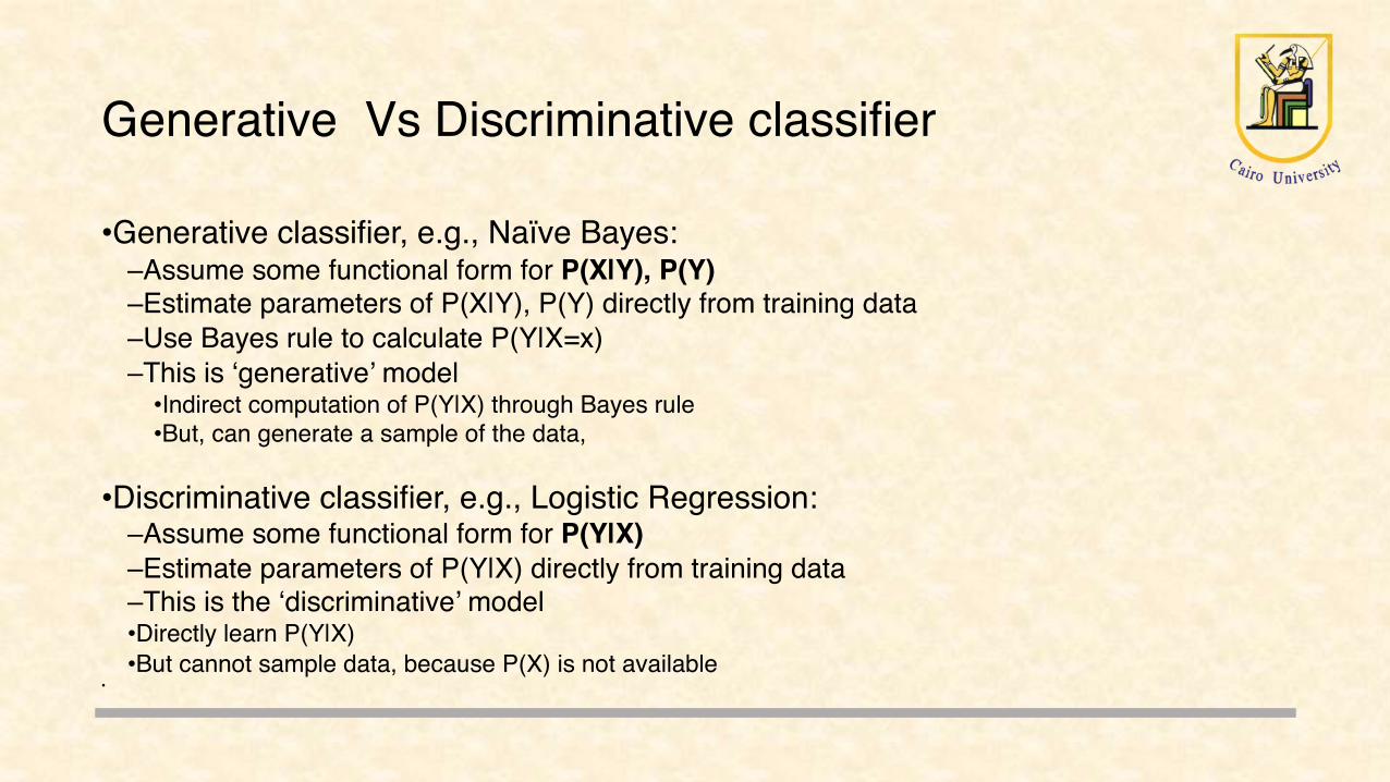
Generative Vs Discriminative classifier

•Generative classifier, e.g., Naïve Bayes:–Assume some functional form for P(X|Y), P(Y)–Estimate parameters of P(X|Y), P(Y) directly from training data–Use Bayes rule to calculate P(Y|X=x)–This is ‘generative’ model

•Indirect computation of P(Y|X) through Bayes rule•But, can generate a sample of the data,

 •Discriminative classifier, e.g., Logistic Regression:

–Assume some functional form for P(Y|X)–Estimate parameters of P(Y|X) directly from training data–This is the ‘discriminative’ model•Directly learn P(Y|X)•But cannot sample data, because P(X) is not available

•

Bayesian Decision Theory

Outline

• What is classification? • Classification by Bayesian Classification • Basic Concepts • Bayes Rule • More General Forms of Bayes Rule • Discriminated Functions • Bayesian Belief Networks

TYPICAL APPLICATIONS OF PRIMAGE PROCESSING EXAMPLE

• Sorting Fish: incoming fish are sorted according to species using optical sensing (sea bass or salmon?)

Feature Extraction

Segmentation

Sensing

• Problem Analysis: ▪ set up a camera and take

some sample images to extract features ▪ Consider features such as

length, lightness, width, number and shape of fins, position of mouth, etc.

What is pattern recognition?

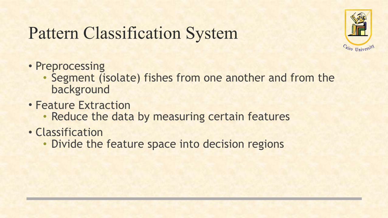
Pattern Classification System

• Preprocessing • Segment (isolate) fishes from one another and from the

background • Feature Extraction

• Reduce the data by measuring certain features • Classification

• Divide the feature space into decision regions

Classification

• Initially use the length of the fish as a possible feature for discrimination

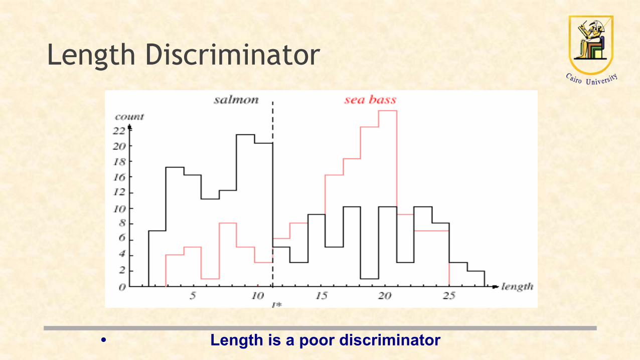
Length Discriminator

• Length is a poor discriminator

Feature Selection

The length is a poor feature alone!

Select the lightness as a possible feature

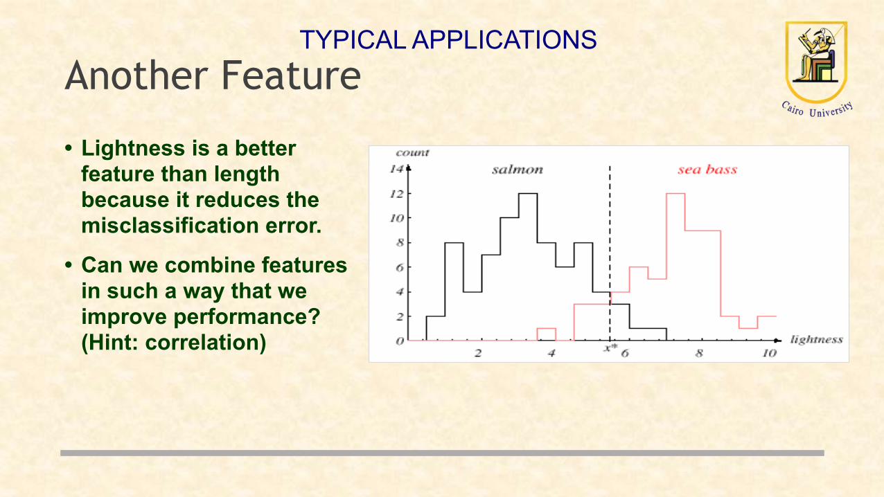
Another Feature

• Lightness is a better feature than length because it reduces the misclassification error.

• Can we combine features in such a way that we improve performance? (Hint: correlation)

TYPICAL APPLICATIONS

Threshold Decision Boundary and Cost Relationship• Move decision boundary toward smaller values of lightness in

order to minimize the cost (reduce the number of sea bass that are classified salmon!)

Task of decision theory

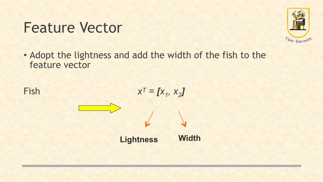
Feature Vector

• Adopt the lightness and add the width of the fish to the feature vector

Fish xT = [x1, x2]

Lightness Width

Width and Lightness Boundary

• Treat features as a N-tuple (two-dimensional vector)

• Create a scatter plot

• Draw a line (regression) separating the two classes

Features

• We might add other features that are not highly correlated with the ones we already have. Be sure not to reduce the performance by adding “noisy features”

• Ideally, you might think the best decision boundary is the one that provides optimal performance on the training data (see the following figure)

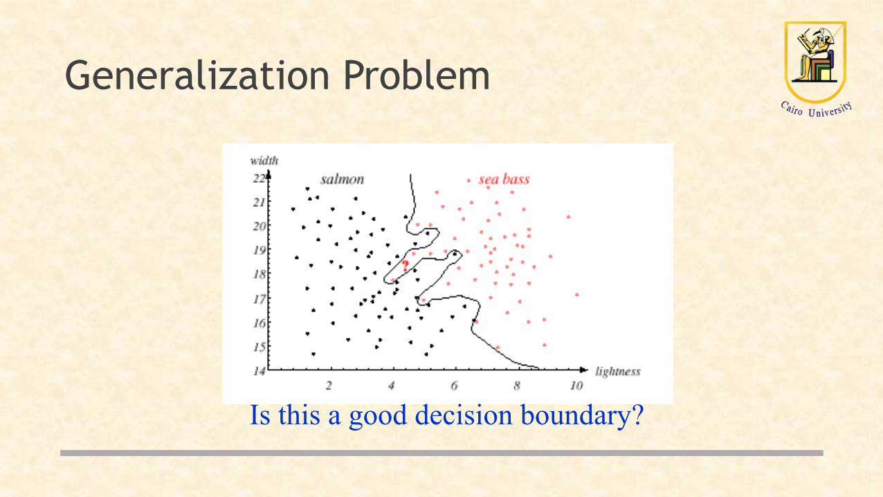
Generalization Problem

Is this a good decision boundary?

Decision Boundary Choice

• Our satisfaction is premature because the central aim of designing a classifier is to correctly classify new (test) input

Issue of generalization!

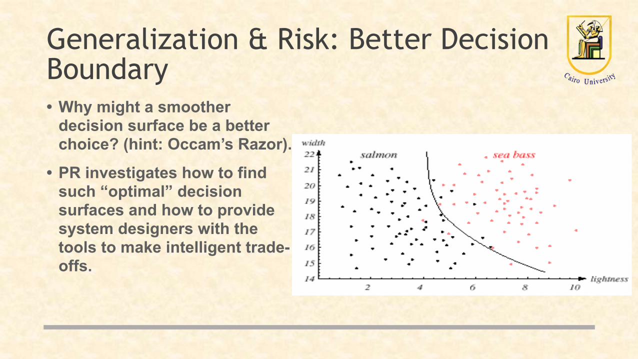
Generalization & Risk: Better Decision Boundary• Why might a smoother

decision surface be a better choice? (hint: Occam’s Razor).

• PR investigates how to find such “optimal” decision surfaces and how to provide system designers with the tools to make intelligent trade-offs.

Need for Probabilistic Reasoning

• Most everyday reasoning is based on uncertain evidence and inferences.

• Classical logic, which only allows conclusions to be strictly true or strictly false, does not account for this uncertainty or the need to weigh and combine conflicting evidence.

• Todays expert systems employed fairly ad hoc methods for reasoning under uncertainty and for combining evidence.

Probabilistic Decision Theory

• Bayesian decision theory is a fundamental statistical approach to the problem of pattern classification.

• Using probabilistic approach to help making decision (e.g., classification) so as to minimize the risk (cost).

• Assume all relevant probability distributions are known (later we will learn how to estimate these from data).

Prior Probability■ State of nature is prior information

○ ω denote the state of nature ■ Model as a random variable, ω:

▪ ω = ω1: the event that the next fish is a sea bass ▪ category 1: sea bass; category 2: salmon

• A priori probabilities: ▪ P(ω1) = probability of category 1 ▪ P(ω2) = probability of category 2 ▪ P(ω1) + P( ω2) = 1 (either ω1 or ω2 must occur)

• Decision rule Decide ω1 if P(ω1) > P(ω2); otherwise, decide ω2

But we know there will be many mistakes ….

http://www.stat.yale.edu/Courses/1997-98/101/ranvar.htm

Class Conditional Probabilities■ A decision rule with only prior information always produces the

same result and ignores measurements.

■ If P(ω1) >> P( ω2), we will be correct most of the time.

• Given a feature, x (lightness), which is a continuous random variable, p(x|ω2) is the class-conditional probability density function:

• p(x|ω1) and p(x|ω2) describe the difference in lightness between populations of sea and salmon.

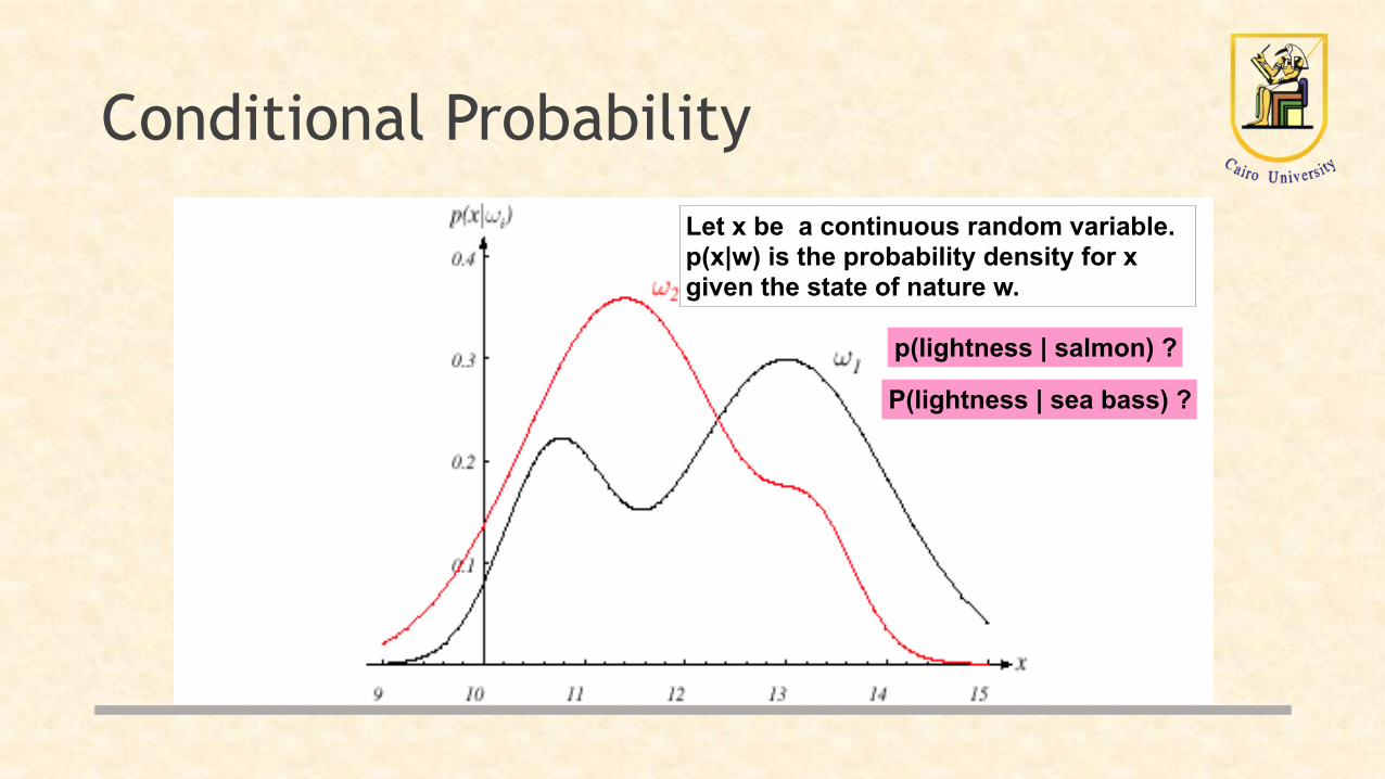
Conditional Probability

p(lightness | salmon) ?

P(lightness | sea bass) ?

Let x be a continuous random variable. p(x|w) is the probability density for x given the state of nature w.

Preliminaries and Notations

:},,,{ 21 ci ωωωω !∈ a state of nature

:)( iP ω prior probability

:x feature vector :)|( ip ωx class-conditional

density :)|( xiP ω posterior probability

Bayes Formula: Combining A prioiri and Conditional Probabilities

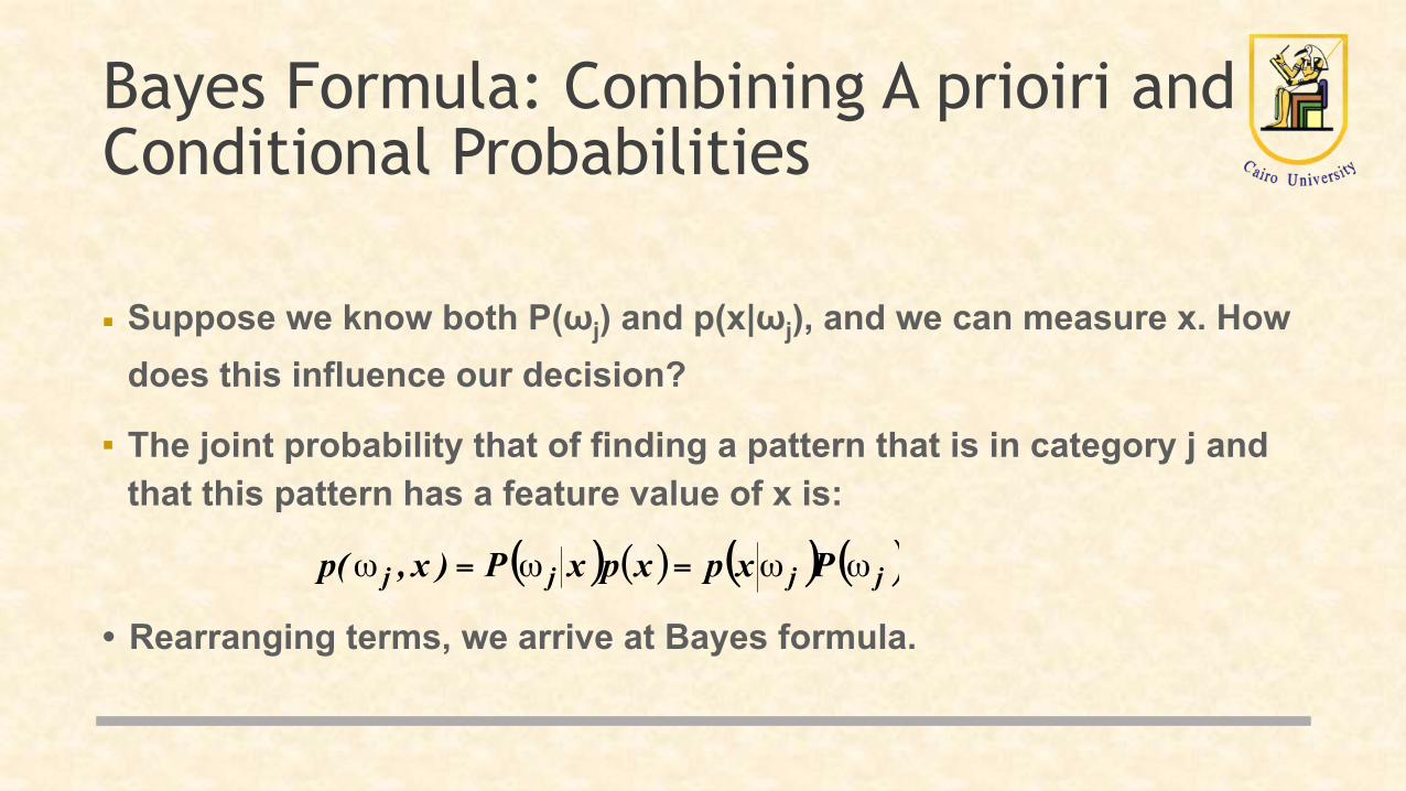
■ Suppose we know both P(ωj) and p(x|ωj), and we can measure x. How does this influence our decision?

■ The joint probability that of finding a pattern that is in category j and that this pattern has a feature value of x is:

( ) ( ) ( ) ( )jjjj PxpxpxP)x,(p ωω=ω=ω

• Rearranging terms, we arrive at Bayes formula.

Casual Formulation

•The prior probability reflects knowledge of the relative frequency of instances of a class •The likelihood is a measure of the probability that a measurement value occurs in a class •The evidence is a scaling term

Posterior Probability■ Bayes formula:

can be expressed in words as:

■ By measuring x, we can convert the prior probability, P(ωj), into a posterior probability, P(ωj|x).

■ Evidence can be viewed as a scale factor and is often ignored in optimization applications (e.g., speech recognition).

( ) ( ) ( )( )xpPxp

xP jjj

ωω=ω

evidencepriorlikelihoodposterior ×

=

Bayes Decision: Choose w1 if P(w1|x) > P(w2|x); otherwise choose w2.

For two categories:

Two Categories

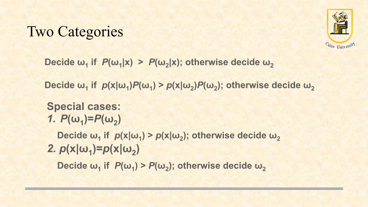
Decide ω1 if P(ω1|x) > P(ω2|x); otherwise decide ω2

Decide ω1 if p(x|ω1)P(ω1) > p(x|ω2)P(ω2); otherwise decide ω2

Special cases: 1. P(ω1)=P(ω2) Decide ω1 if p(x|ω1) > p(x|ω2); otherwise decide ω2 2. p(x|ω1)=p(x|ω2) Decide ω1 if P(ω1) > P(ω2); otherwise decide ω2

Example

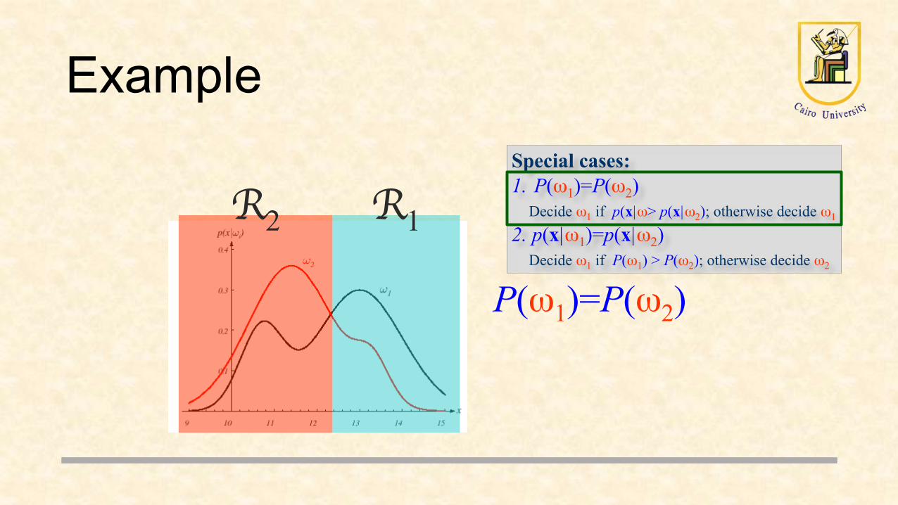
R2

P(ω1)=P(ω2)

R1

Special cases:1. P(ω1)=P(ω2)

Decide ω1 if p(x|ω> p(x|ω2); otherwise decide ω1

2. p(x|ω1)=p(x|ω2)Decide ω1 if P(ω1) > P(ω2); otherwise decide ω2

Example

R1R1R2

R2

P(ω1)=2/3 P(ω2)=1/3

Decide ω1 if p(x|ω1)P(ω1) > p(x|ω2)P(ω2); otherwise decide ω2

Bayes Decision Rule

Posterior Probability

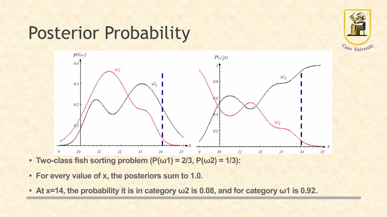
• Two-class fish sorting problem (P(ω1) = 2/3, P(ω2) = 1/3):

• For every value of x, the posteriors sum to 1.0.

• At x=14, the probability it is in category ω2 is 0.08, and for category ω1 is 0.92.

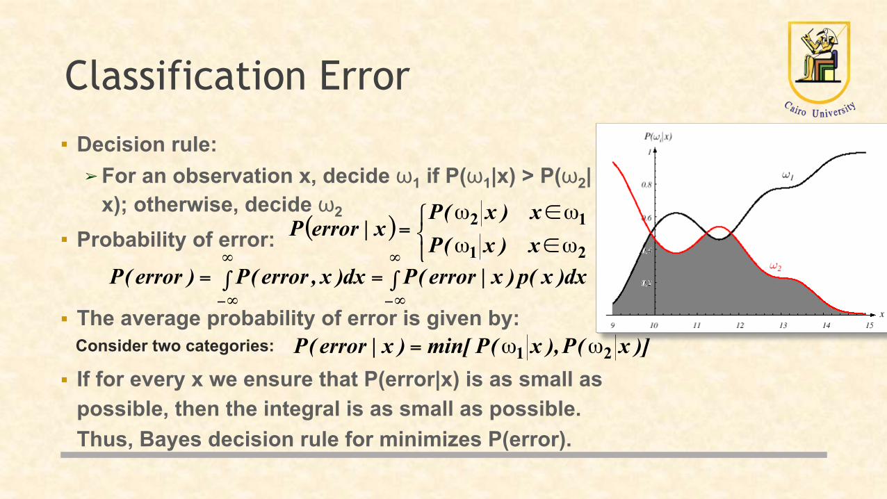
Classification Error■ Decision rule:

➢ For an observation x, decide ω1 if P(ω1|x) > P(ω2|x); otherwise, decide ω2

■ Probability of error:

■ The average probability of error is given by:

■ If for every x we ensure that P(error|x) is as small as possible, then the integral is as small as possible. Thus, Bayes decision rule for minimizes P(error).

( )⎩⎨⎧

ω∈ω

ω∈ω=

21

12

x)x(Px)x(P

x|errorP

∫∫ ==∞

∞−

∞

∞−dx)x(p)x|error(Pdx)x,error(P)error(P

)]x(P),x(Pmin[)x|error(P 21 ωω=Consider two categories:

Generalization of Two-Class Problem

■ Generalization of the preceding ideas: ▪ Use of more than one feature (e.g., length and lightness) ▪ Use more than two states of nature (e.g., N-way classification) ▪ Allowing actions other than a decision to decide on the state of

nature (e.g., rejection: refusing to take an action when alternatives are close or confidence is low)

▪ Introduce a loss of function which is more general than the probability of error (e.g., errors are not equally costly)

▪ Let us replace the scalar x by the vector x in a d-dimensional Euclidean space, Rd, called the feature space.

Decision Regions

} )()(|{ ijgg jii ≠∀>= xxxR

Two-category example

Decision regions are separated by decision boundaries.

The net effect is to divide the feature space into c regions (one for each class). We then have c decision regions separated by decision boundaries.

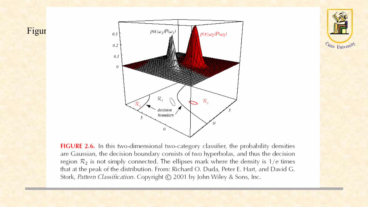
Figure 2.6

Bayesian Decision Theory(Classification)

The Normal Distribution

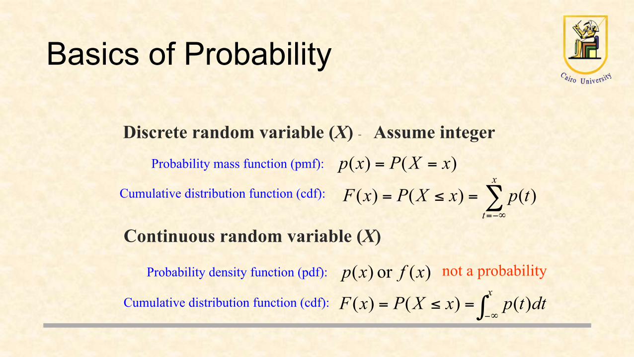
Basics of Probability

Discrete random variable (X) － Assume integer

Continuous random variable (X)

Probability mass function (pmf): )()( xXPxp ==

Cumulative distribution function (cdf): ∑−∞=

=≤=x

t

tpxXPxF )()()(

Probability density function (pdf): )(or )( xfxp

Cumulative distribution function (cdf): ∫ ∞−=≤=x

dttpxXPxF )()()(

not a probability

Introduction to Machine Learning

Thank You …

Inas A. Yassine