Introduction to Logic in Computer Science: Autumn 2007 · Semantics of FOL The semantics of a language deﬁnes the meaning of clauses in that language. In the case of FOL, we do

Tableaux for First-order Logic ILCS 2007

Introduction toLogic in Computer Science: Autumn 2007

Ulle EndrissInstitute for Logic, Language and Computation

University of Amsterdam

Ulle Endriss 1


Tableaux for First-order Logic

The next part of the course will be an introduction to analytictableaux for classical first-order logic:

• Quick review of syntax and semantics of first-order logic

• Quantifier rules for Smullyan-style and KE-style tableaux

• Soundness and completeness proofs

• Automatic generation of countermodels

• Discussion of efficiency issues, undecidability

• Free-variable tableaux to increase efficiency

• Tableaux for first-order logic with equality

• Clause tableaux for input in CNF

Ulle Endriss 2


Syntax of FOL

The syntax of a language defines the way in which basic elements ofthe language may be put together to form clauses of that language.In the case of FOL, the basic ingredients are (besides the logicoperators): variables, function symbols, and predicate symbols. Eachfunction and predicate symbol is associated with an arity n ≥ 0.

Definition 1 (Terms) We inductively define the set of terms asthe smallest set such that:

(1) every variable is a term;

(2) if f is a function symbol of arity k and t1, . . . , tk are terms,then f(t1, . . . , tk) is also a term.

Function symbols of arity 0 are better known as constants.

Ulle Endriss 3


Syntax of FOL (2)

Definition 2 (Formulas) We inductively define the set offormulas as the smallest set such that:

(1) if P is a predicate symbol of arity k and t1 . . . , tk are terms,then P (t1, . . . , tk) is a formula;

(2) if ϕ and ψ are formulas, so are ¬ϕ, ϕ ∧ ψ, ϕ ∨ ψ, and ϕ→ ψ;

(3) if x is a variable and ϕ is a formula, then (∀x)ϕ and (∃x)ϕ arealso formulas.

Syntactic sugar: ϕ↔ ψ ≡ (ϕ→ ψ) ∧ (ψ → ϕ); > ≡ P ∨ ¬P(for an arbitrary 0-place predicate symbol P ); ⊥ ≡ ¬>.

Also recall: atoms, literals, ground terms, bound and freevariables, closed formulas (aka sentences), . . .

Ulle Endriss 4


Semantics of FOL

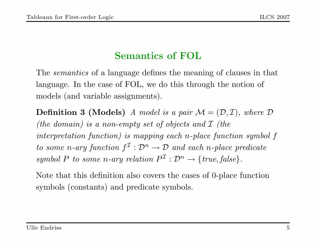
The semantics of a language defines the meaning of clauses in thatlanguage. In the case of FOL, we do this through the notion ofmodels (and variable assignments).

Definition 3 (Models) A model is a pair M = (D, I), where D(the domain) is a non-empty set of objects and I (theinterpretation function) is mapping each n-place function symbol fto some n-ary function fI : Dn → D and each n-place predicatesymbol P to some n-ary relation P I : Dn → {true, false}.

Note that this definition also covers the cases of 0-place functionsymbols (constants) and predicate symbols.

Ulle Endriss 5


Semantics of FOL (2)

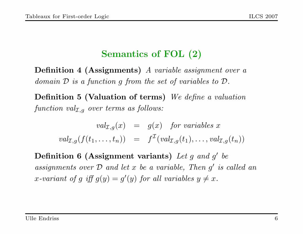
Definition 4 (Assignments) A variable assignment over adomain D is a function g from the set of variables to D.

Definition 5 (Valuation of terms) We define a valuationfunction valI,g over terms as follows:

valI,g(x) = g(x) for variables x

valI,g(f(t1, . . . , tn)) = fI(valI,g(t1), . . . , valI,g(tn))

Definition 6 (Assignment variants) Let g and g′ beassignments over D and let x be a variable, Then g′ is called anx-variant of g iff g(y) = g′(y) for all variables y 6= x.

Ulle Endriss 6



Definition 7 (Satisfaction relation) We write M, g |= ϕ to saythat the formula ϕ is satisfied in the model M = (I,D) under theassignment g. The relation |= is defined inductively as follows:

(1) M, g |= P (t1, . . . , tn) iff P I(valI,g(t1), . . . , valI,g(tn)) = true;

(2) M, g |= ¬ϕ iff not M, g |= ϕ;

(3) M, g |= ϕ ∧ ψ iff M, g |= ϕ and M, g |= ψ;

(4) M, g |= ϕ ∨ ψ iff M, g |= ϕ or M, g |= ψ;

(5) M, g |= ϕ→ ψ iff not M, g |= ϕ or M, g |= ψ;

(6) M, g |= (∀x)ϕ iff M, g′ |= ϕ for all x-variants g′ of g; and

(7) M, g |= (∃x)ϕ iff M, g′ |= ϕ for some x-variant g′ of g.

Ulle Endriss 7



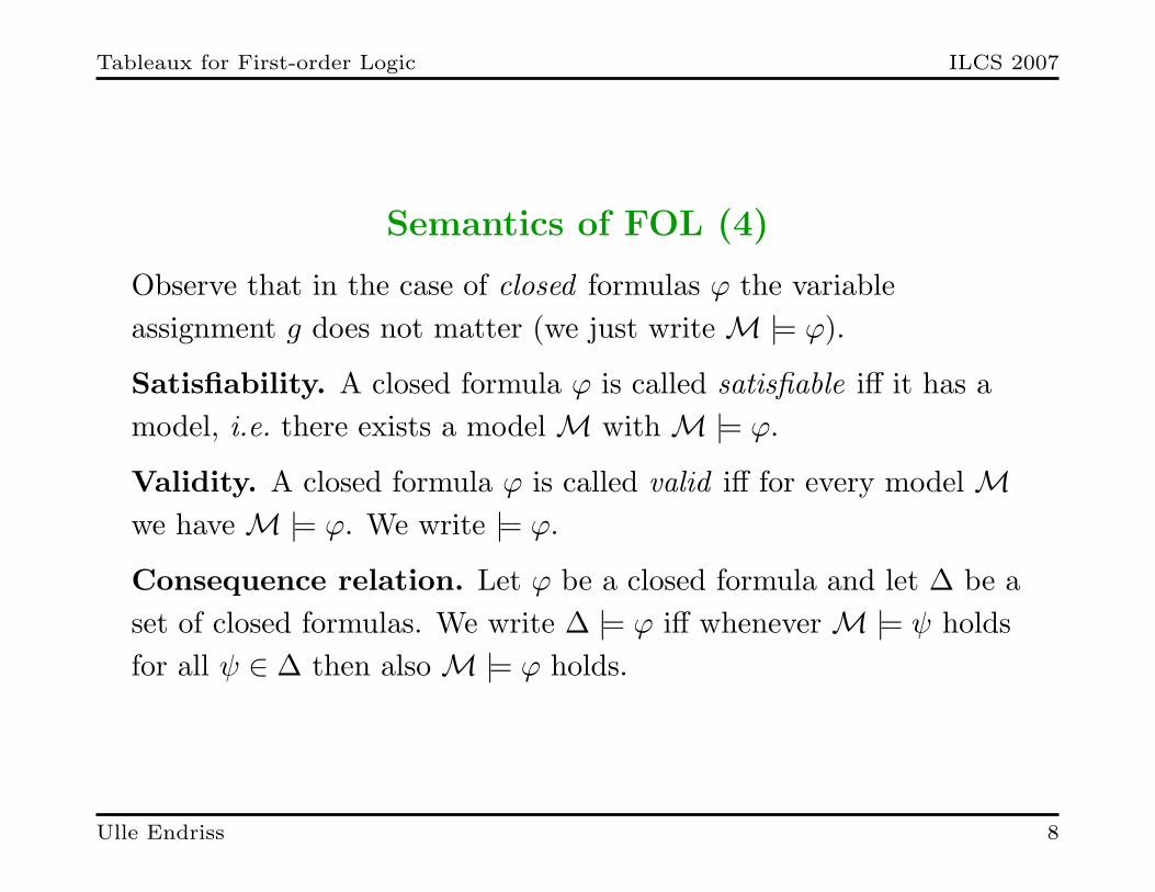
Observe that in the case of closed formulas ϕ the variableassignment g does not matter (we just write M |= ϕ).

Satisfiability. A closed formula ϕ is called satisfiable iff it has amodel, i.e. there exists a model M with M |= ϕ.

Validity. A closed formula ϕ is called valid iff for every model Mwe have M |= ϕ. We write |= ϕ.

Consequence relation. Let ϕ be a closed formula and let ∆ be aset of closed formulas. We write ∆ |= ϕ iff whenever M |= ψ holdsfor all ψ ∈ ∆ then also M |= ϕ holds.

Ulle Endriss 8


Quantifier Rules

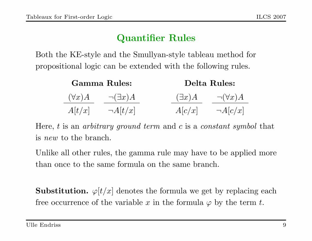
Both the KE-style and the Smullyan-style tableau method forpropositional logic can be extended with the following rules.

Gamma Rules:

(∀x)AA[t/x]

¬(∃x)A¬A[t/x]

Delta Rules:

(∃x)AA[c/x]

¬(∀x)A¬A[c/x]

Here, t is an arbitrary ground term and c is a constant symbol thatis new to the branch.

Unlike all other rules, the gamma rule may have to be applied morethan once to the same formula on the same branch.

Substitution. ϕ[t/x] denotes the formula we get by replacing eachfree occurrence of the variable x in the formula ϕ by the term t.

Ulle Endriss 9


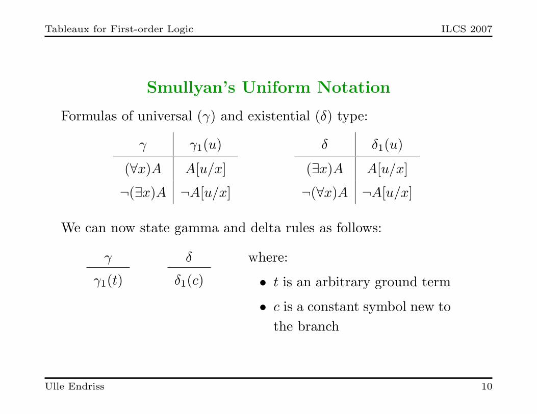
Smullyan’s Uniform Notation

Formulas of universal (γ) and existential (δ) type:

γ γ1(u)

(∀x)A A[u/x]

¬(∃x)A ¬A[u/x]

δ δ1(u)

(∃x)A A[u/x]

¬(∀x)A ¬A[u/x]

We can now state gamma and delta rules as follows:

γ

γ1(t)

δ

δ1(c)

where:

• t is an arbitrary ground term

• c is a constant symbol new tothe branch

Ulle Endriss 10


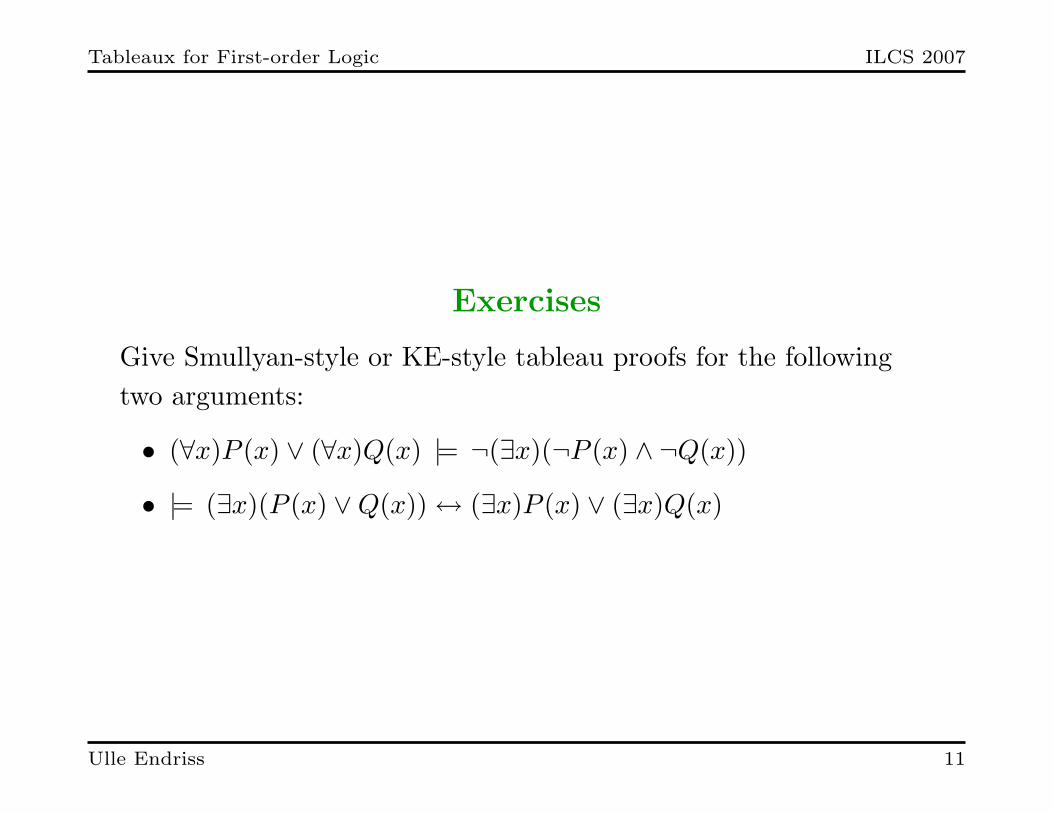
Exercises

Give Smullyan-style or KE-style tableau proofs for the followingtwo arguments:

• (∀x)P (x) ∨ (∀x)Q(x) |= ¬(∃x)(¬P (x) ∧ ¬Q(x))

• |= (∃x)(P (x) ∨Q(x)) ↔ (∃x)P (x) ∨ (∃x)Q(x)

Ulle Endriss 11


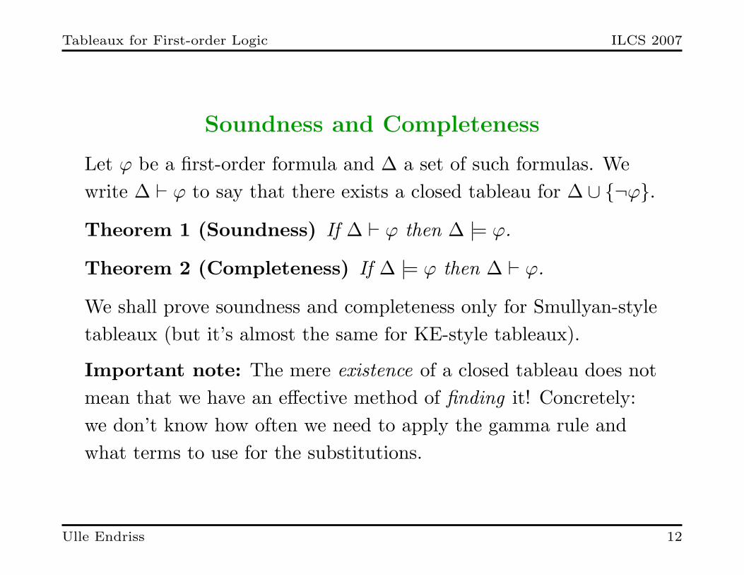
Soundness and Completeness

Let ϕ be a first-order formula and ∆ a set of such formulas. Wewrite ∆ ` ϕ to say that there exists a closed tableau for ∆ ∪ {¬ϕ}.

Theorem 1 (Soundness) If ∆ ` ϕ then ∆ |= ϕ.

Theorem 2 (Completeness) If ∆ |= ϕ then ∆ ` ϕ.

We shall prove soundness and completeness only for Smullyan-styletableaux (but it’s almost the same for KE-style tableaux).

Important note: The mere existence of a closed tableau does notmean that we have an effective method of finding it! Concretely:we don’t know how often we need to apply the gamma rule andwhat terms to use for the substitutions.

Ulle Endriss 12


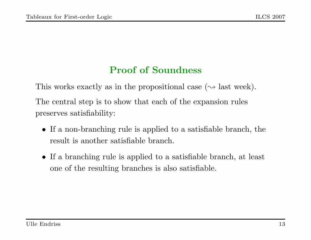
Proof of Soundness

This works exactly as in the propositional case (; last week).

The central step is to show that each of the expansion rulespreserves satisfiability:

• If a non-branching rule is applied to a satisfiable branch, theresult is another satisfiable branch.

• If a branching rule is applied to a satisfiable branch, at leastone of the resulting branches is also satisfiable.

Ulle Endriss 13


Proof of Soundness (cont.)

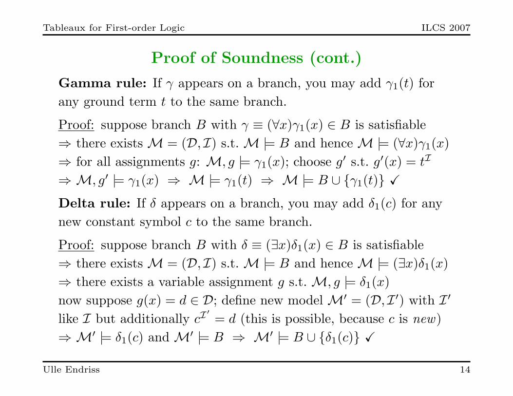
Gamma rule: If γ appears on a branch, you may add γ1(t) forany ground term t to the same branch.

Proof: suppose branch B with γ ≡ (∀x)γ1(x) ∈ B is satisfiable⇒ there exists M = (D, I) s.t. M |= B and hence M |= (∀x)γ1(x)⇒ for all assignments g: M, g |= γ1(x); choose g′ s.t. g′(x) = tI

⇒ M, g′ |= γ1(x) ⇒ M |= γ1(t) ⇒ M |= B ∪ {γ1(t)} X

Delta rule: If δ appears on a branch, you may add δ1(c) for anynew constant symbol c to the same branch.

Proof: suppose branch B with δ ≡ (∃x)δ1(x) ∈ B is satisfiable⇒ there exists M = (D, I) s.t. M |= B and hence M |= (∃x)δ1(x)⇒ there exists a variable assignment g s.t. M, g |= δ1(x)now suppose g(x) = d ∈ D; define new model M′ = (D, I ′) with I ′

like I but additionally cI′= d (this is possible, because c is new)

⇒ M′ |= δ1(c) and M′ |= B ⇒ M′ |= B ∪ {δ1(c)} X

Ulle Endriss 14


Hintikka’s Lemma

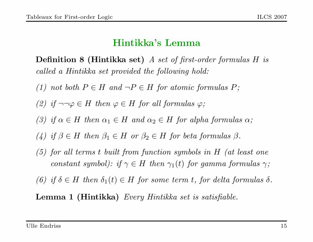
Definition 8 (Hintikka set) A set of first-order formulas H iscalled a Hintikka set provided the following hold:

(1) not both P ∈ H and ¬P ∈ H for atomic formulas P ;

(2) if ¬¬ϕ ∈ H then ϕ ∈ H for all formulas ϕ;

(3) if α ∈ H then α1 ∈ H and α2 ∈ H for alpha formulas α;

(4) if β ∈ H then β1 ∈ H or β2 ∈ H for beta formulas β.

(5) for all terms t built from function symbols in H (at least oneconstant symbol): if γ ∈ H then γ1(t) for gamma formulas γ;

(6) if δ ∈ H then δ1(t) ∈ H for some term t, for delta formulas δ.

Lemma 1 (Hintikka) Every Hintikka set is satisfiable.

Ulle Endriss 15


Proof of Hintikka’s Lemma

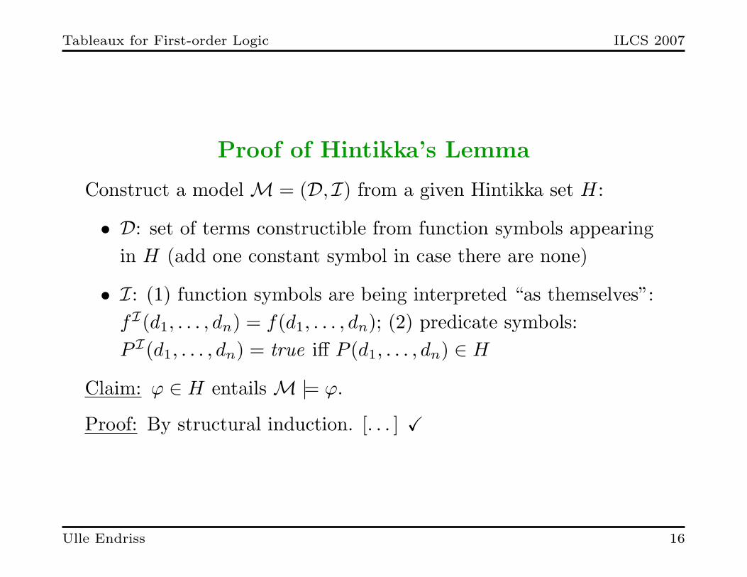
Construct a model M = (D, I) from a given Hintikka set H:

• D: set of terms constructible from function symbols appearingin H (add one constant symbol in case there are none)

• I: (1) function symbols are being interpreted “as themselves”:fI(d1, . . . , dn) = f(d1, . . . , dn); (2) predicate symbols:P I(d1, . . . , dn) = true iff P (d1, . . . , dn) ∈ H

Claim: ϕ ∈ H entails M |= ϕ.

Proof: By structural induction. [. . . ] X

Ulle Endriss 16


Proof of Completeness

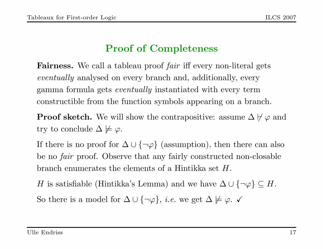
Fairness. We call a tableau proof fair iff every non-literal getseventually analysed on every branch and, additionally, everygamma formula gets eventually instantiated with every termconstructible from the function symbols appearing on a branch.

Proof sketch. We will show the contrapositive: assume ∆ 6` ϕ andtry to conclude ∆ 6|= ϕ.

If there is no proof for ∆ ∪ {¬ϕ} (assumption), then there can alsobe no fair proof. Observe that any fairly constructed non-closablebranch enumerates the elements of a Hintikka set H.

H is satisfiable (Hintikka’s Lemma) and we have ∆ ∪ {¬ϕ} ⊆ H.

So there is a model for ∆ ∪ {¬ϕ}, i.e. we get ∆ 6|= ϕ. X

Ulle Endriss 17


Summary: Basic Tableaux Systems for FOL

• Two tableau methods for first-order logic: Smullyan-style(syntactic branching) and KE-style (semantic branching)

• Soundness and completeness

• Undecidability: gamma rule is the culprit

Ulle Endriss 18


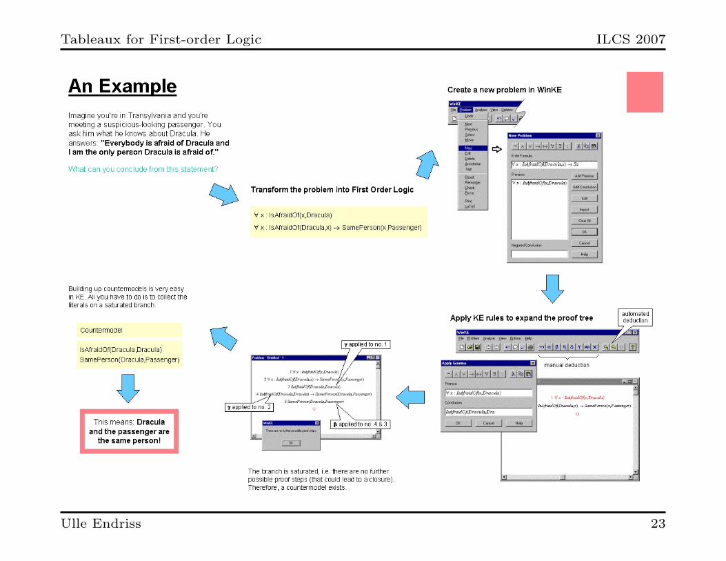
Automatic Generation of Countermodels

Besides deduction and theorem proving, another importantapplication of automated reasoning is model generation.

Using tableaux, we sometimes get termination for failed proofs andcan extract a counterexample (particularly nice for KE).

Ulle Endriss 19


Saturated Branches

An open branch is called saturated iff every non-literal has beenanalysed at least once and, additionally, every gamma formula hasbeen instantiated with every term we can construct using thefunction symbols on the branch.

Failing proofs. A tableau with an open saturated branch cannever be closed, i.e. we can stop an declare the proof a failure.

The solution? This only helps us in special cases though.(A single 1-place function symbol together with a constant isalready enough to construct infinitely many terms . . . )

Propositional logic. In propositional logic (where we have nogamma formulas), after a limited number of steps, every branch willbe either closed or saturated. This gives us a decision procedure.

Ulle Endriss 20


Countermodels

If a KE proof fails with a saturated open branch, you can use it tohelp you define a model M for all the formulas on that branch:

• domain: set of all terms we can construct using the functionsymbols appearing on the branch (so-called Herbrand universe)

• terms are interpreted as themselves

• interpretation of predicate symbols: see literals on branch

In particular, M will be a model for the premises ∆ and thenegated conclusion ¬ϕ, i.e. a counterexample for ∆ |= ϕ.

You can do the same with Smullyan-style tableaux, but for KEdistinct open branches always generate distinct models.

Take care: There’s a bug in WinKE—sometimes, what ispresented as a countermodel is in fact only part of a countermodel(but it can always be extended to an actual model).

Ulle Endriss 21


Exercise

Construct a counterexample for the following argument:

• (∀x)(P (x) ∨Q(x)) |=? (∀x)P (x) ∨ (∀x)Q(x)

Ulle Endriss 22


Ulle Endriss 23


Extensions and Variations

Next we’ll be looking into several extensions and variations of thetableau method for first-order logic:

• Free-variable tableaux to increase efficiency

• Tableaux for first-order logic with equality

• Clause tableaux for input in CNF

Ulle Endriss 24


Efficiency Issues

Due to the undecidability of first-order logic there can be nogeneral method for finding a closed tableau for a given theorem(although its existence is guaranteed by completeness).

Nevertheless, there are some heuristics:

• As in the propositional case, use “deterministic” rules first:propositional rules except PB and the delta rule.

• As in the propositional case, use beta simplification.

• Use the gamma rule a “reasonable” number of times (with“promising” substitutions) before attempting to use PB.

Example: for the automated theorem prover implemented in

WinKE you can choose n, the maximum number of applications

of the gamma rule on a given branch before PB will be used.

• Use analytic PB only.

Ulle Endriss 25


A Problem and an Idea

One of the main drawbacks of either variant of the tableau methodfor FOL, as presented so far, is that for every application of thegamma rule we have to guess a good term for the substitution.

And idea to circumvent this problem would be to try to “postpone”the decision of what substitution to choose until we attempt toclose branches, at which stage we would have to check whetherthere are complementary literals that are unifiable.

Instead of substituting with ground terms we will use free variables.As this would be cumbersome for KE-style tableaux, we will onlypresent free-variable Smullyan-style tableaux.

But first, we need to speak about unification in earnest . . .

Ulle Endriss 26


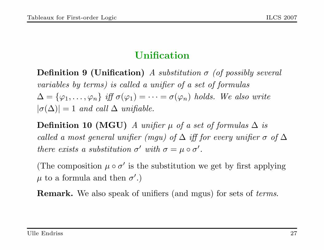
Unification

Definition 9 (Unification) A substitution σ (of possibly severalvariables by terms) is called a unifier of a set of formulas∆ = {ϕ1, . . . , ϕn} iff σ(ϕ1) = · · · = σ(ϕn) holds. We also write|σ(∆)| = 1 and call ∆ unifiable.

Definition 10 (MGU) A unifier µ of a set of formulas ∆ iscalled a most general unifier (mgu) of ∆ iff for every unifier σ of ∆there exists a substitution σ′ with σ = µ ◦ σ′.

(The composition µ ◦ σ′ is the substitution we get by first applyingµ to a formula and then σ′.)

Remark. We also speak of unifiers (and mgus) for sets of terms.

Ulle Endriss 27


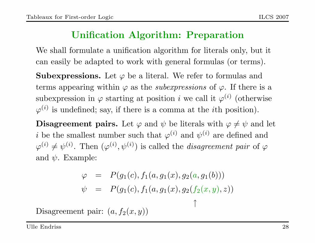
Unification Algorithm: Preparation

We shall formulate a unification algorithm for literals only, but itcan easily be adapted to work with general formulas (or terms).

Subexpressions. Let ϕ be a literal. We refer to formulas andterms appearing within ϕ as the subexpressions of ϕ. If there is asubexpression in ϕ starting at position i we call it ϕ(i) (otherwiseϕ(i) is undefined; say, if there is a comma at the ith position).

Disagreement pairs. Let ϕ and ψ be literals with ϕ 6= ψ and leti be the smallest number such that ϕ(i) and ψ(i) are defined andϕ(i) 6= ψ(i). Then (ϕ(i), ψ(i)) is called the disagreement pair of ϕand ψ. Example:

ϕ = P (g1(c), f1(a, g1(x), g2(a, g1(b)))

ψ = P (g1(c), f1(a, g1(x), g2(f2(x, y), z))

↑Disagreement pair: (a, f2(x, y))

Ulle Endriss 28


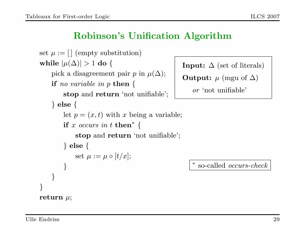
Robinson’s Unification Algorithm

set µ := [ ] (empty substitution)

while |µ(∆)| > 1 do {pick a disagreement pair p in µ(∆);

if no variable in p then {stop and return ‘not unifiable’;

} else {let p = (x, t) with x being a variable;

if x occurs in t then∗ {stop and return ‘not unifiable’;

} else {set µ := µ ◦ [t/x];

}}

}return µ;

Input: ∆ (set of literals)

Output: µ (mgu of ∆)

or ‘not unifiable’

∗ so-called occurs-check

Ulle Endriss 29


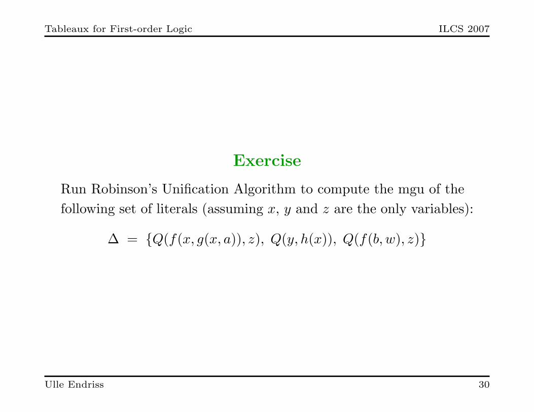
Exercise

Run Robinson’s Unification Algorithm to compute the mgu of thefollowing set of literals (assuming x, y and z are the only variables):

∆ = {Q(f(x, g(x, a)), z), Q(y, h(x)), Q(f(b, w), z)}

Ulle Endriss 30


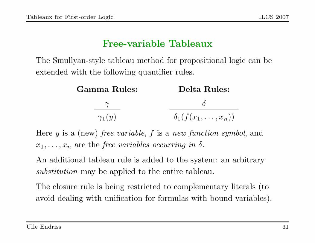
Free-variable Tableaux

The Smullyan-style tableau method for propositional logic can beextended with the following quantifier rules.

Gamma Rules:

γ

γ1(y)

Delta Rules:

δ

δ1(f(x1, . . . , xn))

Here y is a (new) free variable, f is a new function symbol, andx1, . . . , xn are the free variables occurring in δ.

An additional tableau rule is added to the system: an arbitrarysubstitution may be applied to the entire tableau.

The closure rule is being restricted to complementary literals (toavoid dealing with unification for formulas with bound variables).

Ulle Endriss 31


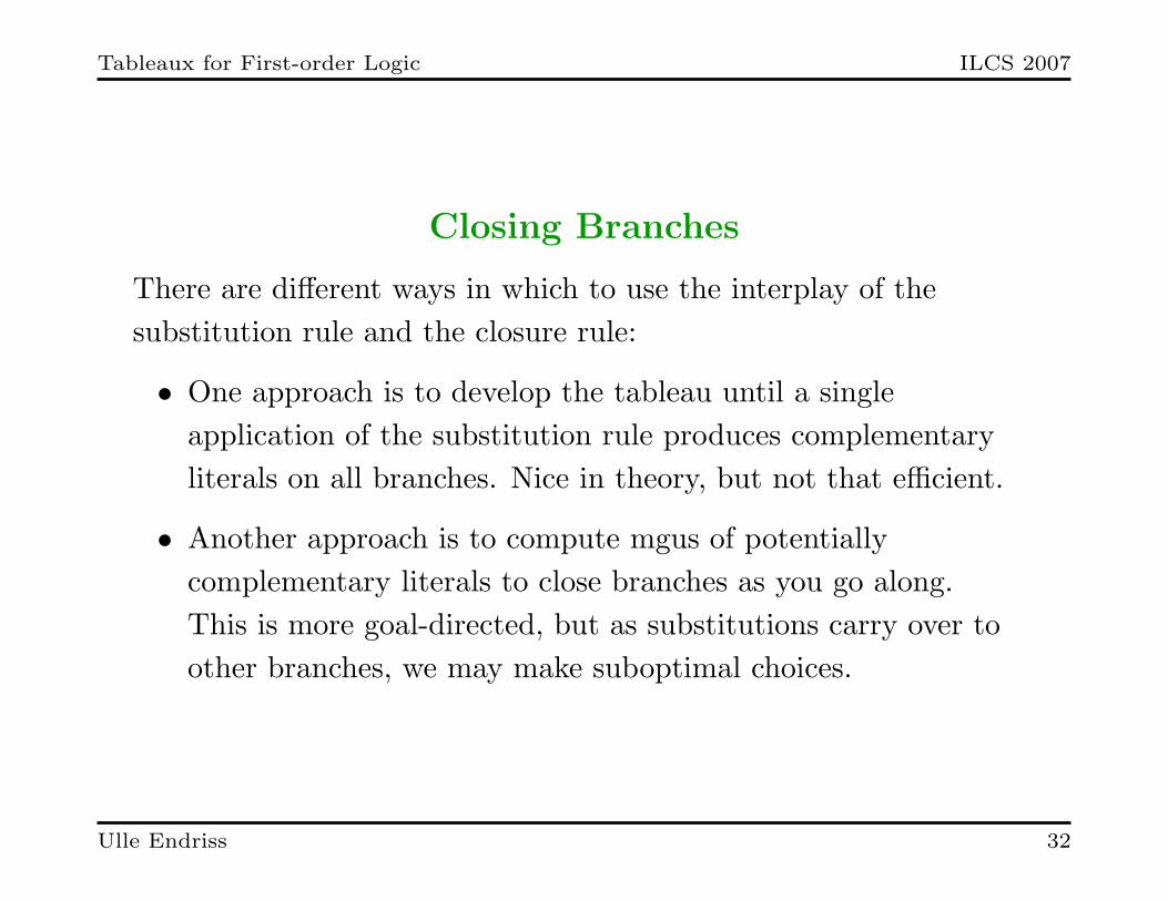
Closing Branches

There are different ways in which to use the interplay of thesubstitution rule and the closure rule:

• One approach is to develop the tableau until a singleapplication of the substitution rule produces complementaryliterals on all branches. Nice in theory, but not that efficient.

• Another approach is to compute mgus of potentiallycomplementary literals to close branches as you go along.This is more goal-directed, but as substitutions carry over toother branches, we may make suboptimal choices.

Ulle Endriss 32


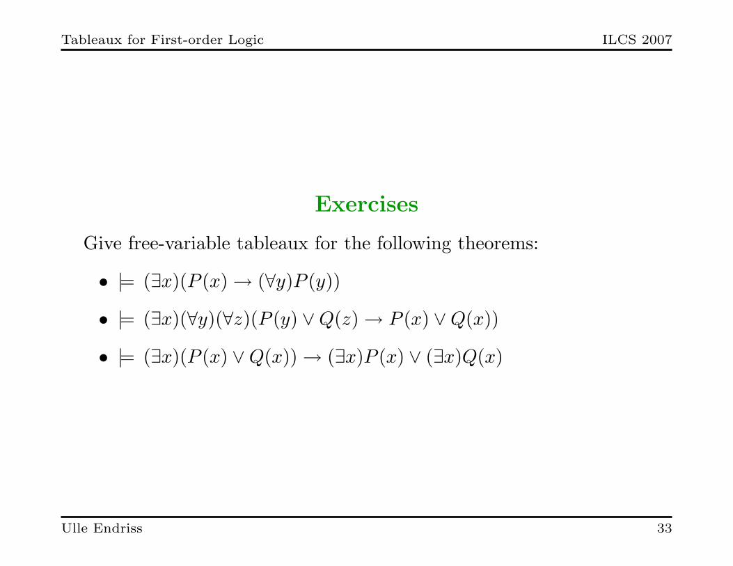
Exercises

Give free-variable tableaux for the following theorems:

• |= (∃x)(P (x) → (∀y)P (y))

• |= (∃x)(∀y)(∀z)(P (y) ∨Q(z) → P (x) ∨Q(x))

• |= (∃x)(P (x) ∨Q(x)) → (∃x)P (x) ∨ (∃x)Q(x)

Ulle Endriss 33


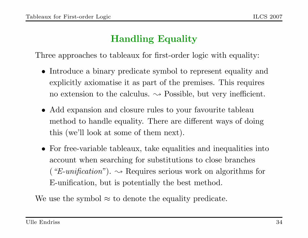
Handling Equality

Three approaches to tableaux for first-order logic with equality:

• Introduce a binary predicate symbol to represent equality andexplicitly axiomatise it as part of the premises. This requiresno extension to the calculus. ; Possible, but very inefficient.

• Add expansion and closure rules to your favourite tableaumethod to handle equality. There are different ways of doingthis (we’ll look at some of them next).

• For free-variable tableaux, take equalities and inequalities intoaccount when searching for substitutions to close branches(“E-unification”). ; Requires serious work on algorithms forE-unification, but is potentially the best method.

We use the symbol ≈ to denote the equality predicate.

Ulle Endriss 34


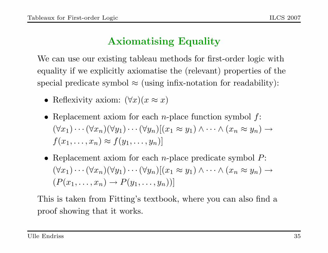
Axiomatising Equality

We can use our existing tableau methods for first-order logic withequality if we explicitly axiomatise the (relevant) properties of thespecial predicate symbol ≈ (using infix-notation for readability):

• Reflexivity axiom: (∀x)(x ≈ x)

• Replacement axiom for each n-place function symbol f :(∀x1) · · · (∀xn)(∀y1) · · · (∀yn)[(x1 ≈ y1) ∧ · · · ∧ (xn ≈ yn) →f(x1, . . . , xn) ≈ f(y1, . . . , yn)]

• Replacement axiom for each n-place predicate symbol P :(∀x1) · · · (∀xn)(∀y1) · · · (∀yn)[(x1 ≈ y1) ∧ · · · ∧ (xn ≈ yn) →(P (x1, . . . , xn) → P (y1, . . . , yn))]

This is taken from Fitting’s textbook, where you can also find aproof showing that it works.

Ulle Endriss 35


Jeffrey’s Tableau Rules for Equality

These are the classical tableau rules for handling equality andapply to ground tableaux:

A(t)t ≈ s

A(s)

A(t)s ≈ t

A(s)

¬(t ≈ t)

×

Exercise: Show |= (a ≈ b) ∧ P (a, a) → P (b, b).

For even just slightly more complex examples, these rules quicklygive rise to a huge search space . . .

Ulle Endriss 36


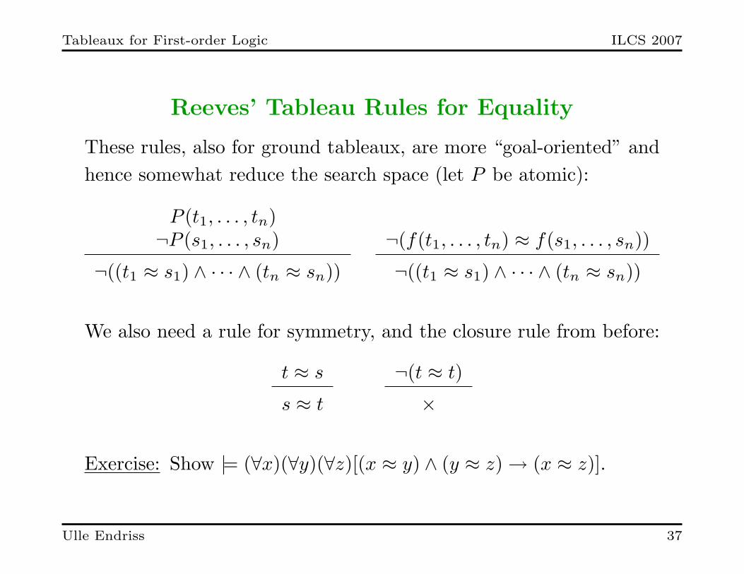
Reeves’ Tableau Rules for Equality

These rules, also for ground tableaux, are more “goal-oriented” andhence somewhat reduce the search space (let P be atomic):

P (t1, . . . , tn)¬P (s1, . . . , sn)

¬((t1 ≈ s1) ∧ · · · ∧ (tn ≈ sn))

¬(f(t1, . . . , tn) ≈ f(s1, . . . , sn))

¬((t1 ≈ s1) ∧ · · · ∧ (tn ≈ sn))

We also need a rule for symmetry, and the closure rule from before:

t ≈ s

s ≈ t

¬(t ≈ t)

×

Exercise: Show |= (∀x)(∀y)(∀z)[(x ≈ y) ∧ (y ≈ z) → (x ≈ z)].

Ulle Endriss 37


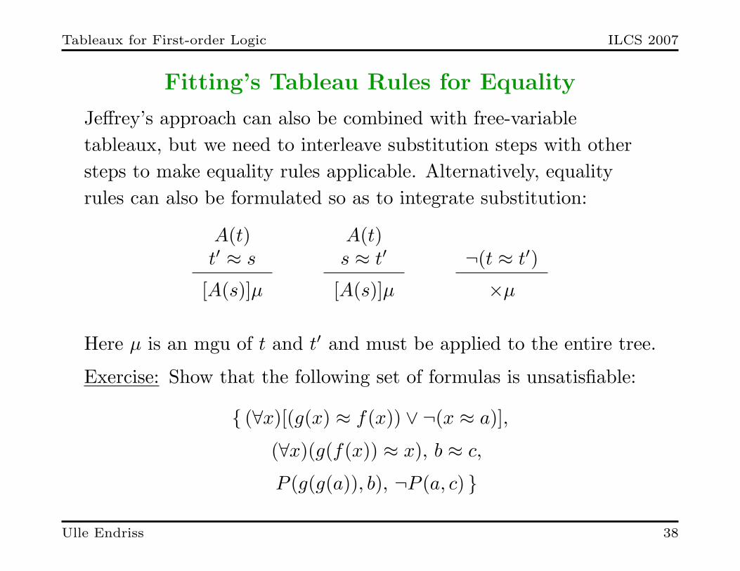
Fitting’s Tableau Rules for Equality

Jeffrey’s approach can also be combined with free-variabletableaux, but we need to interleave substitution steps with othersteps to make equality rules applicable. Alternatively, equalityrules can also be formulated so as to integrate substitution:

A(t)t′ ≈ s

[A(s)]µ

A(t)s ≈ t′

[A(s)]µ

¬(t ≈ t′)

×µ

Here µ is an mgu of t and t′ and must be applied to the entire tree.

Exercise: Show that the following set of formulas is unsatisfiable:

{ (∀x)[(g(x) ≈ f(x)) ∨ ¬(x ≈ a)],

(∀x)(g(f(x)) ≈ x), b ≈ c,

P (g(g(a)), b), ¬P (a, c) }

Ulle Endriss 38


Tableaux and Resolution

The most popular deduction system in automated reasoning is theresolution method (to be discussed briefly later on in the course).

Resolution works for formulas in CNF. This restriction to a normalform makes resolution very efficient. Still, the tableau method hasseveral advantages:

• Tableaux proofs are a lot easier to read than resolution proofs.

• Input may not be in CNF and translation may result in anexponential blow-up.

• For some non-classical logic, translation may be impossible.

Nevertheless, people interested in developing powerful theoremprovers for FOL (rather than in using tableaux as a more generalframework) are often interested in tableaux for CNF, also to allowfor better comparison with resolution.

Ulle Endriss 39


Normal Forms

Recall: Conjunctive Normal Form (CNF) and Disjunctive NormalForm (DNF) for propositional logic

Prenex Normal Form. A FOL formula ϕ is said to be in PrenexNormal Form iff all its quantifiers (if any) “come first”. Thequantifier-free part of ϕ is called the matrix of ϕ.

Every sentence can be transformed into a logically equivalentsentence in Prenex Normal Form.

Ulle Endriss 40


Transformation into Prenex Normal Form

If necessary, rewrite the formula first to ensure that no twoquantifiers bind the same variable and no variable has both a freeand a bound occurrence (variables need to be “named apart”).

¬(∀x)A ≡ (∃x)¬A

((∀x)A) ∧B ≡ (∀x)(A ∧B)

((∀x)A) ∨B ≡ (∀x)(A ∨B)

¬(∃x)A ≡ (∀x)¬A

((∃x)A) ∧B ≡ (∃x)(A ∧B)

((∃x)A) ∨B ≡ (∃x)(A ∨B)

etc.

To avoid making mistakes, formulas involving → or ↔ should firstbe translated into formulas using only ¬, ∧ and ∨ (and quantifiers).

Ulle Endriss 41


Skolemisation

Skolemisation is the process of removing existential quantifiers froma formula in Prenex Normal Form (without affecting satisfiability).

Algorithm. Given: a formula in Prenex Normal Form.

(1) If necessary, turn the formula into a sentence by adding (∀x) infront for every free variable x (“universal closure”).

(2) While there are still existential quantifiers, repeat: replace

• (∀x1) · · · (∀xn)(∃y)ϕ with

• (∀x1) · · · (∀xn)ϕ[f(x1, . . . , xn)/y],where f is a new function symbol.

Ulle Endriss 42


Skolemisation (cont.)

Definition 11 (Skolem Normal Form) A formula ϕ is said tobe in Skolem Normal Form (SNF) iff it is of the following form:

ϕ = (∀x1)(∀x2) · · · (∀xn)ϕ′,

where ϕ′ is a quantifier-free formula in CNF (with n ∈ N0).

Theorem 3 (Skolemisation) For every formula ϕ there exists aformula ϕsk in SNF such that ϕ is satisfiable iff ϕsk is satisfiable.ϕsk can be obtained from ϕ through the process of Skolemisation.

Proof: By induction over the sequence of transformation steps inthe Skolemisation algorithm [details omitted].

Note that ϕ and ϕsk are not (necessarily) equivalent.

Ulle Endriss 43


Exercise

Compute the Skolem Normal Form of the following formula:

(∀x)(∃y)[P (x, g(y)) → ¬(∀x)Q(x)]

Ulle Endriss 44


Clauses

Clauses. A clause is a set of literals. Logically, it corresponds tothe disjunction of these literals.

Sets of clauses. A set of clauses logically corresponds to theconjunction of the clauses in the set.

This means, any formula in Skolem Normal Form can be rewrittenas a set of clauses. Variables are understood to be implicitlyuniversally quantified. Example:

{ {P (x), Q(y)}, {¬P (f(y))} } ∼ (∀x)(∀y)[(P (x)∨Q(y))∧¬P (f(y))]

Ulle Endriss 45


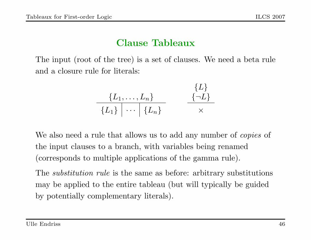
Clause Tableaux

The input (root of the tree) is a set of clauses. We need a beta ruleand a closure rule for literals:

{L1, . . . , Ln}{L1} · · · {Ln}

{L}{¬L}×

We also need a rule that allows us to add any number of copies ofthe input clauses to a branch, with variables being renamed(corresponds to multiple applications of the gamma rule).

The substitution rule is the same as before: arbitrary substitutionsmay be applied to the entire tableau (but will typically be guidedby potentially complementary literals).

Ulle Endriss 46


Clause Tableaux: Alternative Presentation

The presentation on the previous slide attempts to be as close aspossible to what we have done before, but the following alternativepresentation is more common:

• Initialise the tableau with > and keep the set of clauses S to beshown unsatisfiable separate.

• Applying an extension rule means choosing a branch B and anew instance {L1, . . . , Ln} of a clause in S, and then appendingn children below B and labelling them with {L1} to {Ln}.

• Close branches (on literals) using suitable mgu’s as usual.

Observe how this extension rule combines beta and gamma rules.

Ulle Endriss 47


Exercises

Give a closed tableau for the following set of clauses:

• {{P (x), Q(x)}, {¬Q(x),¬R(x)}, {¬P (a)}, {R(x)}}

Give a proof using clause tableaux for the following theorem:

• |= (∃x)(∀y)(∀z)(P (y) ∨Q(z) → P (x) ∨Q(x))

Ulle Endriss 48


Guiding Proofs

Even for clause tableaux, the search space is generally still huge.A lot of research has gone into finding refinements of the basicprocedure to guide proof search. For instance:

• A connection tableau is a clause tableau in which every non-leafnode labelled with a literal L has a child labelled with thecomplement of L.

• A clause tableau is called regular iff no branch contains morethan one copy of the same literal.

Completeness can still be guaranteed if we restrict search to regularconnection tableaux. See the handbook chapter by Hahnle (2001)for a precise statement of this result.

Ulle Endriss 49


Summary: Extensions and Variations

• Free-variable tableaux: postpone instantiations and close byunification (; compute mgus with Robinson’s algorithm)

• Handling equality: several approaches, including several waysof defining additional expansion rules

• Clause tableaux: simplified system for clauses rather thangeneral formulas (; requires translation into SNF)

• Much of the material covered can be found in:

– R. Hahnle. Tableaux and Related Methods. In: A. Robinsonand A. Voronkov (eds.), Handbook of Automated Reasoning,Elsevier Science and MIT Press, 2001.

The material on handling equality is taken from:

– B. Beckert. Semantic Tableaux with Equality. Journal ofLogic and Computation, 7(1):39–58, 1997.

Ulle Endriss 50

Documents

Introduction to Logic in Computer Science: Autumn 2007 · Semantics of FOL The semantics of a language deﬁnes the meaning of clauses in that language. In the case of FOL, we do