Embed Size (px)
Citation preview

Home Page JJ J I IIILFP
Go Back Full Screen Close 1 of 280 Quit
Introduction to (Logic and Functional)Programming
http://www.cse.iitd.ac.in/ sak/courses/ilfp/2014-15.index.html
S. Arun-KumarDepartment of Computer Science and Engineering
I. I. T. Delhi, Hauz Khas, New Delhi 110 016.
March 17, 2015

Home Page JJ J I IIILFP
Go Back Full Screen Close 2 of 280 Quit
Contents
1 Lecture 1: Introduction 5
2 Lecture 2: Functional Programming 13
3 Lecture 3: Standard ML Overview 21
4 Lecture 4: Standard ML Computations 37
5 Lecture 5: Standard ML Scope Rules 54
6 Lecture 6: Sample Sort Programs 80
6.1 Insertion Sort . . . . . . . . . . . . . . . . . . . . . . . . . . . . . . . . . . . . . . . . . . . . . 81
6.2 Selection Sort . . . . . . . . . . . . . . . . . . . . . . . . . . . . . . . . . . . . . . . . . . . . . 84
7 Lecture 7: Higher-order Functions 91
8 Lecture 8: Datatypes 108
9 Lecture 9: Information Hiding 121
10 Lecture 10: Abstract Data Types to Modularity 131

Home Page JJ J I IIILFP
Go Back Full Screen Close 3 of 280 Quit
11 Lecture 11: Signatures, Structures & Functors 139
11.1 Axiomatic Specifications . . . . . . . . . . . . . . . . . . . . . . . . . . . . . . . . . . . . . . . 148
11.1.1 The Stack Datatype . . . . . . . . . . . . . . . . . . . . . . . . . . . . . . . . . . . . . . 148
11.2 Closing Equational Specifications . . . . . . . . . . . . . . . . . . . . . . . . . . . . . . . . . . 162
12 Lecture 12: Example: Tautology Checking 179
13 Lecture 13: Example: Tautology Checking (Contd) 215
14 Lecture 14: The Pure Untyped Lambda Calculus: Syntax 227
15 Lecture 15: The Pure Untyped Lambda Calculus: Basics 230
16 Lecture 16: Notions of Reduction 244
17 Lecture 17: Confluence Definitions 256
18 Lecture 18: The Church-Rosser Property 262
19 Lecture 19: Confluence Characterizations 270
20 Lecture 25 276

Home Page JJ J I IIILFP
Go Back Full Screen Close 5 of 280 Quit
1. Lecture 1: Introduction
Lecture 1: IntroductionTuesday 26 July 2011
Home Page JJ J I IIILFP
Go Back Full Screen Close 6 of 280 Quit
Programming and Algorithms• A computation is a sequence of transformations carried out mechani-
cally by means of a number of predefined rules of transformation onfinite discrete data.•Computations are specified with the help of programs written in a pro-
gramming language.•Algorithms studies specific classes of problems for which programs
may be written on some some universal machine.• Programming is concerned with the logical aspects of program organi-
zation.1. Draws on the study of algorithms to choose efficient data structures
and high-performance algorithms2. Main purpose is to provide concepts and methods for writing pro-
grams correctly, legibly in a way that is easy to modify and reuse.

Home Page JJ J I IIILFP
Go Back Full Screen Close 7 of 280 Quit
Program Specification•How do we specify what to expect from a program?•How do we associate what we expect from a program with a precise
description of what the program computes?•How can we ensure that the program is correct with respect to a given
specification?
These questions can be rigorously answered only by means of a formalmathematical specification and by establishing a formal relationship be-tween the specification and the program.
•Unfortunately, the state of art of these processes is such that they can be doneonly for small programs.•Without sufficient automation of formal reasoning methods these cannot be
done for huge industry scale programs.

Home Page JJ J I IIILFP
Go Back Full Screen Close 8 of 280 Quit
Programming languages History• A continuous effort to abstract high-level concepts in order to escape
low-level details and idiosyncracies of particular machines.– machine language (the use of mnemonics)– assembly language (assemblers)– FORTRAN (compilers)– LISP (interpreters)– Pascal (compiler on a virtual machine)– PROLOG (Abstract machines)– Smalltalk (OO with mutable objects)– ML (Memory abstraction)

Home Page JJ J I IIILFP
Go Back Full Screen Close 9 of 280 Quit
Imperative Programming•Most conventional programming languages (e.g. C, C++, Java)• Evolved from the Von-Neumann architecture (machine, assembly,
FORTRAN)• Principally rely on state changes (visible updation of memory) through
side-effects• Far removed from mathematics (e.g. x = x+1).•Not referentially transparent: the same function placed in different con-
texts behaves differently (side-effects on global variables, aliasingproblems etc.).

Home Page JJ J I IIILFP
Go Back Full Screen Close 10 of 280 Quit
Chronology of Programming Languages

Home Page JJ J I IIILFP
Go Back Full Screen Close 13 of 280 Quit
2. Lecture 2: Functional Programming
Lecture 2: Functional ProgrammingWednesday 27 July 2011

Home Page JJ J I IIILFP
Go Back Full Screen Close 14 of 280 Quit
Functional Programming• A program consists entirely of functions (some may depend on others previously defined). The
“main” program is also a function.• The “main” function is given input values and the result of evaluating it
is the output.•Most functional progrmaming languages are interactive.• The notion of function in a pure functional language is the mathematical
notion of function.

Home Page JJ J I IIILFP
Go Back Full Screen Close 15 of 280 Quit
Imperative vs. Functional• Imperative programs rely on “side-effects” and state updation. There
are no side-effects in “pure” functional programs.• Side-effects in imperative programs are mainly due to assignment com-
mands (either direct or indirect). There is no assignment command inpure functional languages.•Most imperative programmers rely on iterative loops. There is no it-
eration mechanism in a pure functional program. Instead recursion isused.• Variables in imperative programs tend to change values over time.
There is no change in the values of variables in a pure functional pro-gram. Variables are constants.

Home Page JJ J I IIILFP
Go Back Full Screen Close 16 of 280 Quit
Referential TransparencyDefinition 2.1 An expression is referentially transparent if it can be re-placed by its value in a program without changing the behaviour of theprogram in any way.
In a pure functional language all functions are referentially transparent.Hence• programs are mathematically more tractable than imperative ones.• compiler optimizations such as common sub-expression elimination,
code movement etc. can be incorporated without any static analysis.• Any expression anywhere may be replaced by another expression
which has the same value.In most imperative languages (because of assignment, and side-effectsto non-local variables) there is no (guarantee of) referential transparency.

Home Page JJ J I IIILFP
Go Back Full Screen Close 17 of 280 Quit
Higher-order functions & ModularityHigher Order. Higher order functions characterise most functional pro-
gramming. It leads to compact and concise code.Modularity. Modularity can be built into a pure functional languageObjected-orientedness. Object-oriented features require state updation
and can be obtained only by destroying referential transparency. Soa pure functional programming language cannot be object-oriented,though it can be modular.

Home Page JJ J I IIILFP
Go Back Full Screen Close 18 of 280 Quit
Imperative featuresInput/Output. All input-output and file-handling (esp. in the Von Neu-
mann framework) is inherently imperative.Object-Orientation. Object oriented features require updation of state
and are hence better served by imperative features.
So most functional languages need to have certain imperative features.

Home Page JJ J I IIILFP
Go Back Full Screen Close 21 of 280 Quit
3. Lecture 3: Standard ML Overview
Lecture 3: Standard ML OverviewFriday 29 July 2011

Home Page JJ J I IIILFP
Go Back Full Screen Close 22 of 280 Quit
SML: Overview(Impure) FunctionalStrongly and statically typedType inferencingParameterised TypesParametric polymorphismModularity

Home Page JJ J I IIILFP
Go Back Full Screen Close 23 of 280 Quit
SML: FunctionalBased on the model of evaluating expressions as opposed to the model ofexecuting sequences of commands found in imperative languages.
Strongly and statically typedType inferencingParameterised TypesParameterised TypesParametric polymorphismModularity

Home Page JJ J I IIILFP
Go Back Full Screen Close 24 of 280 Quit
SML: Strong Static TypingDefinition 3.1 A language is statically typed if every expression in thelanguage is assigned a type at compile-time.
Definition 3.2 A language is strongly typed if the language requires theprovision of a type-checker which ensures that no type errors will occurat run-time.
Each expression in the ML language is assigned a type at compile-timedescribing the possible set of values it can evaluate to, and no runtimetype errors occur.(Impure) Functional
Type inferencing
Parameterised Types
Parameterised Types
Parametric polymorphism
Modularity
Home Page JJ J I IIILFP
Go Back Full Screen Close 25 of 280 Quit
SML: Parameterised TypesML allows the use of parameterised types which allows a single implemen-tation to be applied to all structures which are instances of the parametrictype. For this purpose ML also has the notion of a type variable.
• Facilitates parametric polymorphism•Reduces duplication of similar code and allows code reuse.
(Impure) Functional
Type inferencing
Parameterised Types
Parametric polymorphism
Modularity

Home Page JJ J I IIILFP
Go Back Full Screen Close 26 of 280 Quit
SML: Type inferencingExcept in a few instances, ML is capable of deducing the types of identi-fiers from the context. There is no need to declare every identifier before it isused.Type-inferencing also works on parametric and polymorphic types in sucha way that ML• assigns the most general parametric polymorphic type to the expres-
sion at compile-time and• ensures that each run-time value produced by the expression is an
appropriate instance of the polymorphic type assigned to it.(Impure) Functional
Strongly and statically typed
Parameterised Types
Parametric polymorphism
Modularity
Home Page JJ J I IIILFP
Go Back Full Screen Close 27 of 280 Quit
SML: Parametric PolymorphismA function gets a polymorphic type when it can operate uniformly overany value of any given type.
Example 3.3 One can define types of the form stack(’a) where ’a isa type variable, for stacks of all types including stacks of complex user-defined data structures and types.The operations defined for stack(’a) work equally well on all instancesof the type.(Impure) Functional
Strongly and statically typed
Type inferencing
Parameterised Types
Modularity

Home Page JJ J I IIILFP
Go Back Full Screen Close 28 of 280 Quit
SML: ModularityA state-of-the-art module system, based on the notions of structures(containing the actual code), signatures (the type of structures) andfunctors (creation of parameterised structures from one or more otherparametrised structures without the need for writing new code).(Impure) Functional
Strongly and statically typed
Type inferencing
Parameterised Types
Parametric polymorphism

Home Page JJ J I IIILFP
Go Back Full Screen Close 29 of 280 Quit
SML: Overview Summary 1(Impure) Functional. Based on the model of evaluating expressions (as op-
posed to the model of executing sequences of commands found in impera-tive languages)
Strongly and statically typed. Each expression in the language is as-signed a type describing the possible set of values it can evaluate to,and type checking at the time of compilation ensures that no runtimetype errors occur.
Type inferencing. Except in a few instances, ML is capable of deducingthe types of identifiers from the context. There is no need to declare everyidentifier before it is used.

Home Page JJ J I IIILFP
Go Back Full Screen Close 30 of 280 Quit
SML: Overview Summary 2Parametric polymorphism. A function gets a polymorphic type when it
can operate uniformly over any value of any given type.Modularity. A state-of-the-art module system, based on the notions of
structures (containing the actual code), signatures (the type of struc-tures) and functors (parametrized structures).
Home Page JJ J I IIILFP
Go Back Full Screen Close 31 of 280 Quit
Functional Pseudocode for writing algorithms
An algorithm will be written in a mixture of English and standard mathematical notation (usually calledpseudo-code). Usually,
• algorithms written in a natural language are often ambiguous
• mathematical notation is not ambiguous, but still cannot be understood by machine
• algorithms written by us use various mathematical properties. We know them, but the machinedoesn’t.
• Even mathematical notation is often not quite precise and certain intermediate objects or steps are leftto the understanding of the reader (e.g. the use of “· · · ” and “...”).
However
• Functional pseudo-code avoids most such implicit assumptions and attempts to make definitions moreprecise (e.g. the use of induction).
• Functional pseudo-code is still concise though more formal than standard mathematical notation.
• However functional pseudo-code is not formal enough to be termed a programming language (e.g. itdoes not satisfy strict grammatical rules and neither is it linear as most formal languages are).
• But functional pseudo-code is precise enough to analyse the correctness and complexity of an algorithm,whereas standard mathematical notation may mask many important details.
•We may freely borrow from the notation of the functional programming language to express variousdata-structuring features.

Home Page JJ J I IIILFP
Go Back Full Screen Close 32 of 280 Quit
An Example
Suppose Real.Math.sqrtwere not available to us!
isqrt(n) of a non-negative integer n is the integer k ≥ 0 such that k2≤ n < (k + 1)2
That is,
isqrt(n) =
⊥ if n < 0k otherwise
where0 ≤ k2
≤ n < (k + 1)2
This value of k is unique!
0 ≤ k2≤ n < (k + 1)2
⇒ 0 ≤ k ≤√
n < k + 1⇒ 0 ≤ k ≤ n
Strategy. Use this fact to close in on the value of k. Start with the interval [l,u] = [0,n] and try to shrink ittill it collapses to the interval [k, k] which contains a single value.
If n = 0 then isqrt(n) = 0.Otherwise with [l,u] = [0,n] and
l2 ≤ n < u2
use one or both of the following to shrink the interval [l,u].

Home Page JJ J I IIILFP
Go Back Full Screen Close 33 of 280 Quit
• if (l + 1)2≤ n then try [l + 1,u]
otherwise l2 ≤ n < (l + 1)2 and k = l
• if u2 > n then try [l,u − 1]otherwise (u − 1)2
≤ n < u2 and k = u − 1
isqrt(n) =
⊥ if n < 00 if n = 0shrink(n, 0,n) if n > 0
where
shrink(n, l,u) =
l if l = ushrink(n, l + 1,u) if l < u and (l + 1)2
≤ nl if l < u and (l + 1)2 > nshrink(n, l,u − 1) if l < u and u2 > nu − 1 if l < u and (u − 1)2
≤ n⊥ if l > u
In the above algorithm the function isqrt uses the function shrink which is recursively defined. Beginningwith an initial closed interval [0,n], shrink reduces the size of the interval by 1 i each recursive call. Thecomplexity of the algorithm is therefore O(n) where n is the input to the function isqrt.
A better algorithm would be as follows. Here the interval is “halved” with each recursive evaluation ofshrink

Home Page JJ J I IIILFP
Go Back Full Screen Close 34 of 280 Quit
isqrt(n) =
⊥ if n < 00 if n = 0shrink(n, 0,n) if n > 0
where
shrink(n, l,u) =
l if l = u or u = l + 1shrink(n,m,u) if l < u and m2
≤ nshrink(n, l,m) if l < u and m2 > n⊥ if l > u
where
m = b(l + u)/2c
Another Example

Home Page JJ J I IIILFP
Go Back Full Screen Close 35 of 280 Quit
( ∗ Program f o r generat ing primes upto some number ∗ )
fun primeWRT (m, [ ] ) = t rue| primeWRT (m, h : : t ) =
i f m mod h = 0 then f a l s ee l s e primeWRT (m, t )
fun generateFrom ( P , m, n ) =i f m > n then Pe l s e i f primeWRT (m, P )then (
generateFrom ( (m: : P ) , m+2 , n ))
e l s e generateFrom ( P , m+2 , n )
fun primesUpto n = i f n < 2 then [ ]e l s e i f n=2 then [ 2 ]e l s e i f ( n mod 2 = 0) then primesUpto ( n−1)e l s e generateFrom ( [ 2 ] , 3 , n ) ;

Home Page JJ J I IIILFP
Go Back Full Screen Close 37 of 280 Quit
4. Lecture 4: Standard ML Computations
Lecture 4: Standard ML ComputationsTuesday 02 Aug 2011

Home Page JJ J I IIILFP
Go Back Full Screen Close 38 of 280 Quit
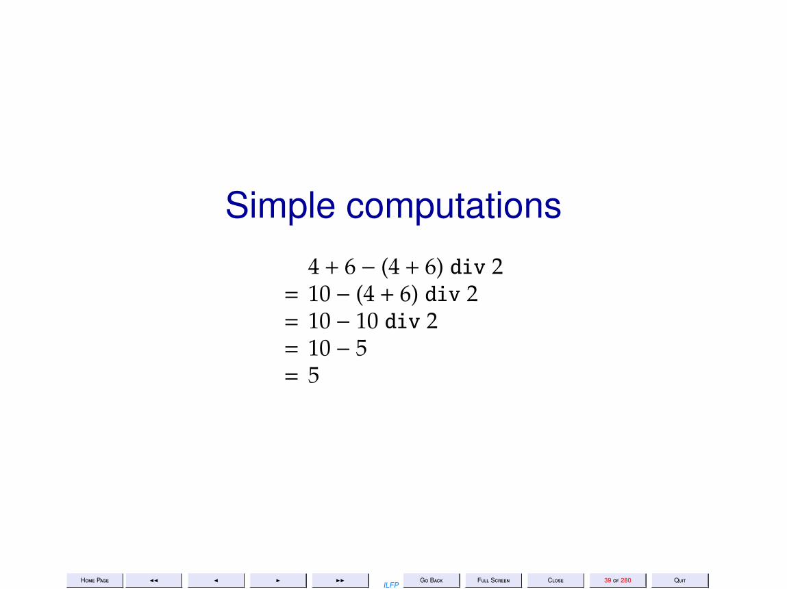
Computations: SimpleFor most simple expressions it is• left to right, and• top to bottom
except when
• presence of brackets• precedence of operators
determine otherwise.
Hence
Home Page JJ J I IIILFP
Go Back Full Screen Close 39 of 280 Quit
Simple computations
4 + 6 − (4 + 6) div 2= 10 − (4 + 6) div 2= 10 − 10 div 2= 10 − 5= 5
Home Page JJ J I IIILFP
Go Back Full Screen Close 40 of 280 Quit
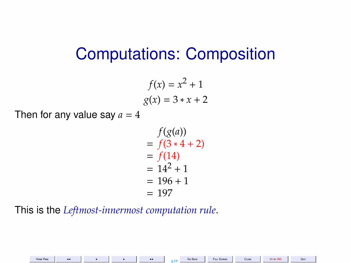
Computations: Composition
f (x) = x2 + 1g(x) = 3 ∗ x + 2
Then for any value say a = 4
f (g(a))= f (3 ∗ 4 + 2)= f (14)= 142 + 1= 196 + 1= 197
This is the Leftmost-innermost computation rule.

Home Page JJ J I IIILFP
Go Back Full Screen Close 41 of 280 Quit
Composition: Alternative
f (x) = x2 + 1g(x) = 3 ∗ x + 2
Why not the following?f (g(a))
= g(4)2 + 1= (3 ∗ 4 + 2)2 + 1= (12 + 2)2 + 1= 142 + 1= 196 + 1= 197
This is the Leftmost-outermost computation rule.

Home Page JJ J I IIILFP
Go Back Full Screen Close 42 of 280 Quit
Compositions: Compare
f (x) = x2 + 1g(x) = 3 ∗ x + 2
Leftmost-innermost computation Leftmost-outermost computationf (g(a)) f (g(a))
= f (3 ∗ 4 + 2) = g(4)2 + 1= f (14) = (3 ∗ 4 + 2)2 + 1
= (12 + 2)2 + 1= 142 + 1 = 142 + 1= 196 + 1 = 196 + 1= 197 = 197

Home Page JJ J I IIILFP
Go Back Full Screen Close 43 of 280 Quit
Compositions: CompareQuestion 1: Which is more correct? Why?Question 2: Which is easier to implement?Question 3: Which is more efficient?

Home Page JJ J I IIILFP
Go Back Full Screen Close 44 of 280 Quit
Computations in SML: CompositionA computation of f (g(a)) proceeds thus:• g(a) is evaluated to some value, say b• f (b) is next evaluated
Home Page JJ J I IIILFP
Go Back Full Screen Close 45 of 280 Quit
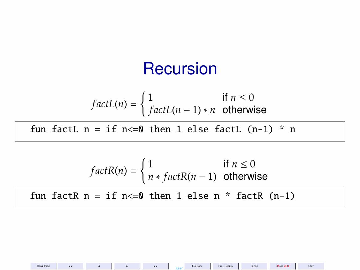
Recursion
f actL(n) =
1 if n ≤ 0f actL(n − 1) ∗ n otherwise
fun factL n = if n<=0 then 1 else factL (n-1) * n
f actR(n) =
1 if n ≤ 0n ∗ f actR(n − 1) otherwise
fun factR n = if n<=0 then 1 else n * factR (n-1)

Home Page JJ J I IIILFP
Go Back Full Screen Close 46 of 280 Quit
Recursion: Left
f actL(4)= ( f actL(4 − 1) ∗ 4)= ( f actL(3) ∗ 4)= (( f actL(3 − 1) ∗ 3) ∗ 4)= (( f actL(2) ∗ 3) ∗ 4)= ((( f actL(2 − 1) ∗ 2) ∗ 3) ∗ 4)= · · ·

Home Page JJ J I IIILFP
Go Back Full Screen Close 47 of 280 Quit
Recursion: Right
f actR(4)= (4 ∗ f actR(4 − 1))= (4 ∗ f actR(3))= (4 ∗ (3 ∗ f actR(3 − 1)))= (4 ∗ (3 ∗ f actR(2)))= (4 ∗ (3 ∗ (2 ∗ f actR(2 − 1))))= · · ·

Home Page JJ J I IIILFP
Go Back Full Screen Close 48 of 280 Quit
Factorial: Tail Recursion 1• The recursive call precedes the multiplication operation. Change it!•Define a state variable p which contains the product of all the values
that one must remember•Reorder the computation so that the computation of p is performed
before the recursive call.• For that redefine the function in terms of p.

Home Page JJ J I IIILFP
Go Back Full Screen Close 49 of 280 Quit
Factorial: Tail Recursion 2f actL2(n) =
1 if n ≤ 0f actL tr(n, 1) otherwise
where
f actL tr(n, p) =
p if n ≤ 0f actL tr(n − 1,np) otherwise
fun factL2 n = if n <= 0 then 1
else let fun factL_tr (n, p) =
if n <= 0 then p
else factL_tr (n-1, n*p)
in factL_tr(n, 1)
end

Home Page JJ J I IIILFP
Go Back Full Screen Close 50 of 280 Quit
A Tail-Recursive Computation
f actL2(4); f actL tr(4, 1); f actL tr(3, 4); f actL tr(2, 12); f actL tr(1, 24); f actL tr(0, 24); 24

Home Page JJ J I IIILFP
Go Back Full Screen Close 51 of 280 Quit
Factorial: IssuesCorrectness : Prove (by induction on n) that for all n ≥ 0, f actL2(n) = n!.Termination : Prove by induction on n that every computation of f actL2
terminates.Space complexity : Prove that S f actL2(n) = O(1) (as against S f actL(n) ∝
n).Time complexity : Prove that T f actL2(n) = O(n)
Home Page JJ J I IIILFP
Go Back Full Screen Close 54 of 280 Quit
5. Lecture 5: Standard ML Scope Rules
Lecture 5: Standard ML Scope RulesWednesday 03 Aug 2011

Home Page JJ J I IIILFP
Go Back Full Screen Close 55 of 280 Quit
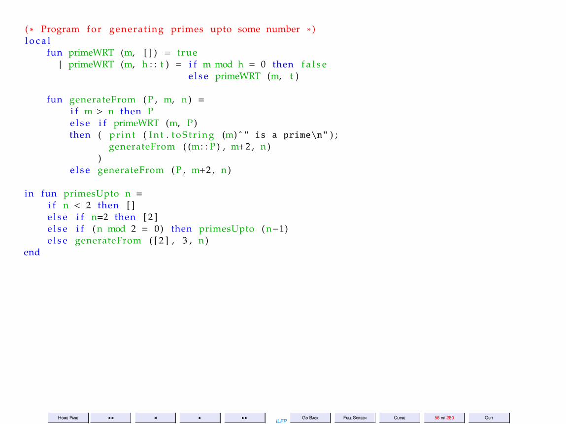
( ∗ Program f o r generat ing primes upto some number ∗ )
fun primeWRT (m, [ ] ) = t rue| primeWRT (m, h : : t ) =
i f m mod h = 0 then f a l s ee l s e primeWRT (m, t )
fun generateFrom ( P , m, n ) =i f m > n then Pe l s e i f primeWRT (m, P )then (
generateFrom ( (m: : P ) , m+2 , n ))
e l s e generateFrom ( P , m+2 , n )
fun primesUpto n = i f n < 2 then [ ]e l s e i f n=2 then [ 2 ]e l s e i f ( n mod 2 = 0) then primesUpto ( n−1)e l s e generateFrom ( [ 2 ] , 3 , n ) ;
Home Page JJ J I IIILFP
Go Back Full Screen Close 56 of 280 Quit
( ∗ Program f o r generat ing primes upto some number ∗ )l o c a l
fun primeWRT (m, [ ] ) = t rue| primeWRT (m, h : : t ) = i f m mod h = 0 then f a l s e
e l s e primeWRT (m, t )
fun generateFrom ( P , m, n ) =i f m > n then Pe l s e i f primeWRT (m, P )then ( p r i n t ( I n t . t o S t r i n g (m) ˆ " is a prime\n" ) ;
generateFrom ( (m: : P ) , m+2 , n ))
e l s e generateFrom ( P , m+2 , n )
in fun primesUpto n =i f n < 2 then [ ]e l s e i f n=2 then [ 2 ]e l s e i f ( n mod 2 = 0) then primesUpto ( n−1)e l s e generateFrom ( [ 2 ] , 3 , n )
end
Home Page JJ J I IIILFP
Go Back Full Screen Close 57 of 280 Quit
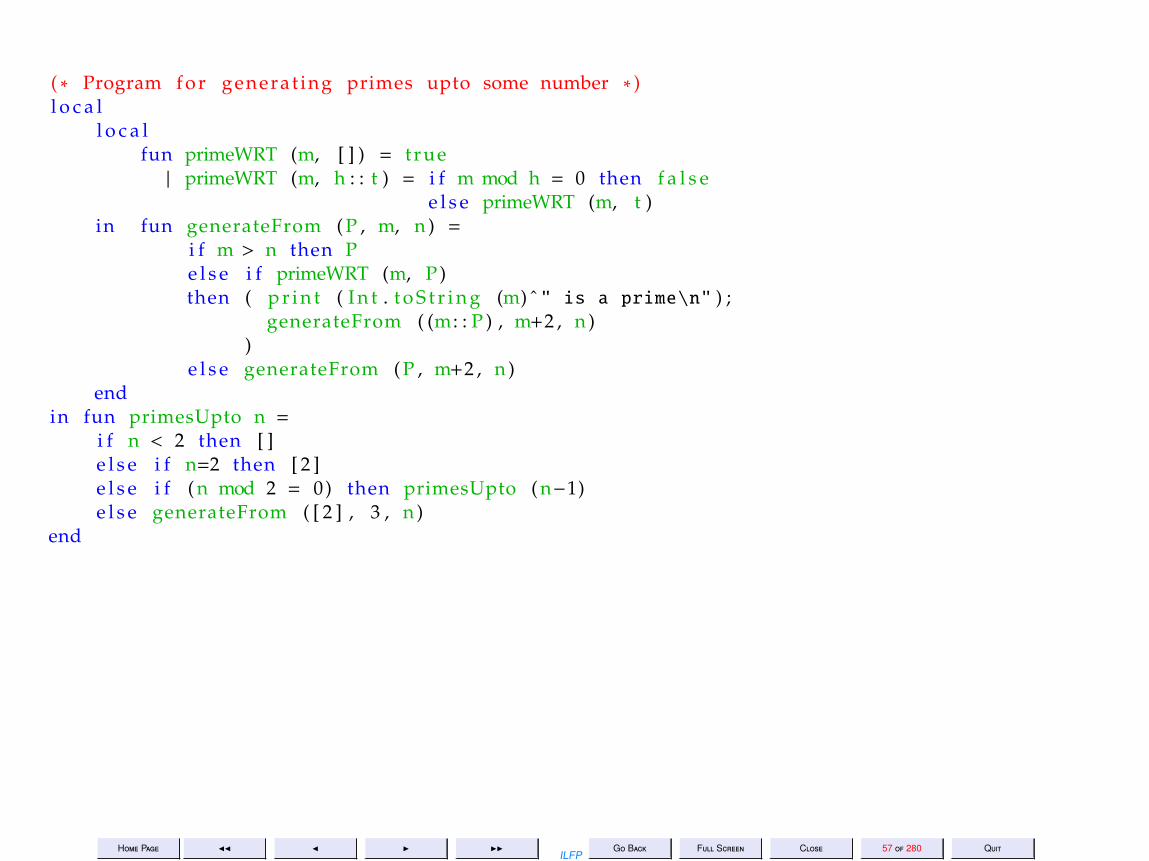
( ∗ Program f o r generat ing primes upto some number ∗ )l o c a l
l o c a lfun primeWRT (m, [ ] ) = t rue| primeWRT (m, h : : t ) = i f m mod h = 0 then f a l s e
e l s e primeWRT (m, t )in fun generateFrom ( P , m, n ) =
i f m > n then Pe l s e i f primeWRT (m, P )then ( p r i n t ( I n t . t o S t r i n g (m) ˆ " is a prime\n" ) ;
generateFrom ( (m: : P ) , m+2 , n ))
e l s e generateFrom ( P , m+2 , n )end
in fun primesUpto n =i f n < 2 then [ ]e l s e i f n=2 then [ 2 ]e l s e i f ( n mod 2 = 0) then primesUpto ( n−1)e l s e generateFrom ( [ 2 ] , 3 , n )
end

Home Page JJ J I IIILFP
Go Back Full Screen Close 58 of 280 Quit
( ∗ Program f o r generat ing primes upto some number ∗ )fun primesUpto n =
i f n < 2 then [ ]e l s e i f n=2 then [ 2 ]e l s e i f ( n mod 2 = 0) then primesUpto ( n−1)e l s e l e t fun primeWRT (m, [ ] ) = t rue
| primeWRT (m, h : : t ) =i f m mod h = 0 then f a l s ee l s e primeWRT (m, t ) ;
fun generateFrom ( P , m, n ) =i f m > n then Pe l s e i f primeWRT (m, P )then ( p r i n t ( I n t . t o S t r i n g (m) ˆ " is a prime\n" ) ;
generateFrom ( (m: : P ) , m+2 , n ))
e l s e generateFrom ( P , m+2 , n )in generateFrom ( [ 2 ] , 3 , n )end

Home Page JJ J I IIILFP
Go Back Full Screen Close 59 of 280 Quit
( ∗ Program f o r generat ing primes upto some number ∗ )fun primesUpto n =
i f n < 2 then [ ]e l s e i f n=2 then [ 2 ]e l s e i f ( n mod 2 = 0) then primesUpto ( n−1)e l s e l e t fun generateFrom ( P , m, n ) =
l e t fun primeWRT (m, [ ] ) = t rue| primeWRT (m, h : : t ) =
i f m mod h = 0 then f a l s ee l s e primeWRT (m, t )
in i f m > n then Pe l s e i f primeWRT (m, P )then ( p r i n t ( I n t . t o S t r i n g (m) ˆ " is a prime\n" ) ;
generateFrom ( (m: : P ) , m+2 , n ))
e l s e generateFrom ( P , m+2 , n )end
in generateFrom ( [ 2 ] , 3 , n )end

Home Page JJ J I IIILFP
Go Back Full Screen Close 60 of 280 Quit
Disjoint Scopeslet
in
end
val x = 10;fun fun1 y =
let...
in...
end
fun fun2 z =let ...in ...end
fun1 (fun2 x)

Home Page JJ J I IIILFP
Go Back Full Screen Close 61 of 280 Quit
Nested Scopeslet
in
end
fun1 x
val x = 10;fun fun1 y =
let
val x = 15
inx + y
end

Home Page JJ J I IIILFP
Go Back Full Screen Close 62 of 280 Quit
Overlapping Scopeslet
in
end
val x = 10;fun fun1 y =
...
...
...
...
fun1 (fun2 x)

Home Page JJ J I IIILFP
Go Back Full Screen Close 63 of 280 Quit
Spannninglet
in
end
val x = 10;fun fun1 y =
...
...
fun fun2 z =
...
...
fun1 (fun2 x)

Home Page JJ J I IIILFP
Go Back Full Screen Close 64 of 280 Quit
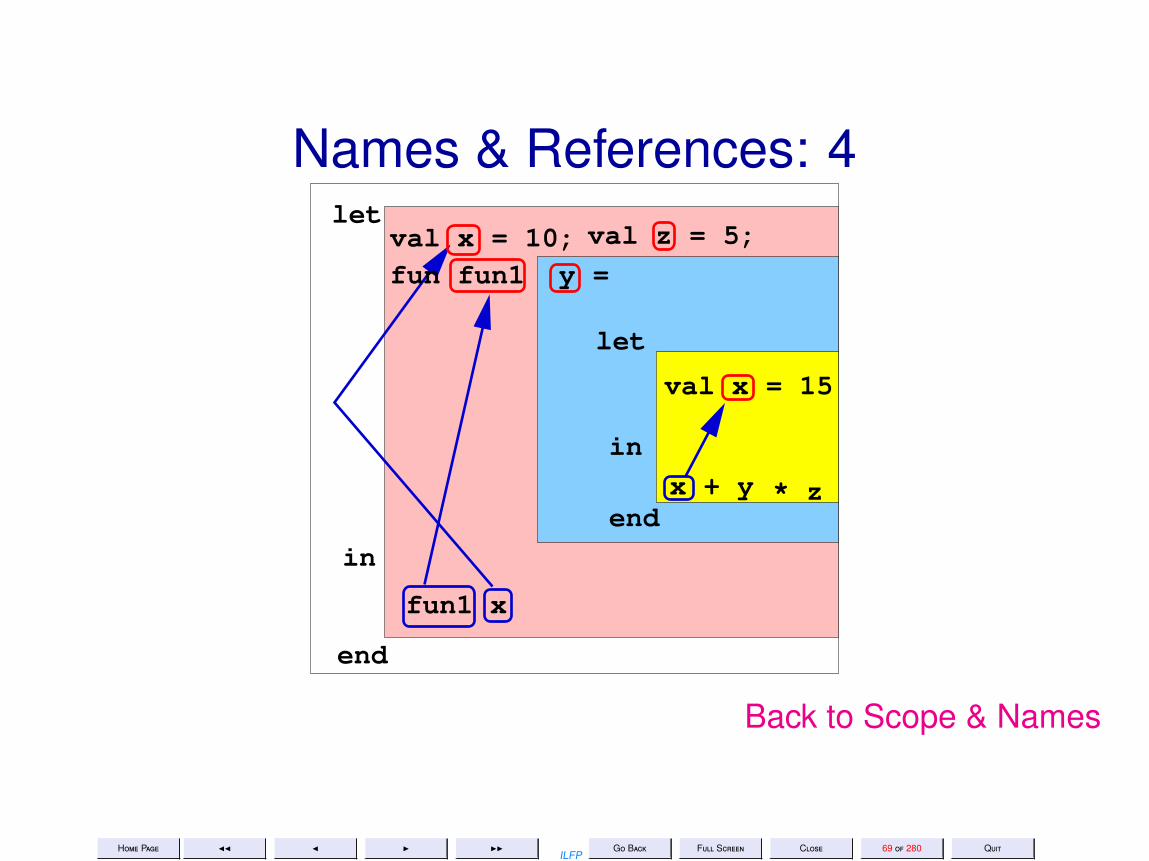
Scope & Names• A name may occur either as being defined or as a use of a previously
defined name• The same name may be used to refer to different objects.• The use of a name refers to the textually most recent definition in the
innermost enclosing scope
diagram

Home Page JJ J I IIILFP
Go Back Full Screen Close 65 of 280 Quit
Names & References: 0let
in
end
fun1 x
val x = 10;fun fun1 y =
let
val x = 15
inx + y
end
val z = 5;
* z
Back to Scope & Names

Home Page JJ J I IIILFP
Go Back Full Screen Close 66 of 280 Quit
Names & References: 1let
in
end
fun1 x
val x = 10;fun fun1 y =
let
val x = 15
inx + y
end
val z = 5;
* z
Back to Scope & Names
Home Page JJ J I IIILFP
Go Back Full Screen Close 67 of 280 Quit
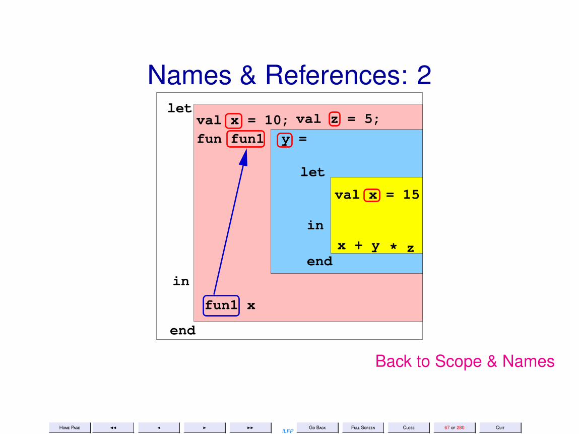
Names & References: 2let
in
end
fun1 x
val x = 10;fun fun1 y =
let
val x = 15
inx + y
end
val z = 5;
* z
Back to Scope & Names
Home Page JJ J I IIILFP
Go Back Full Screen Close 68 of 280 Quit
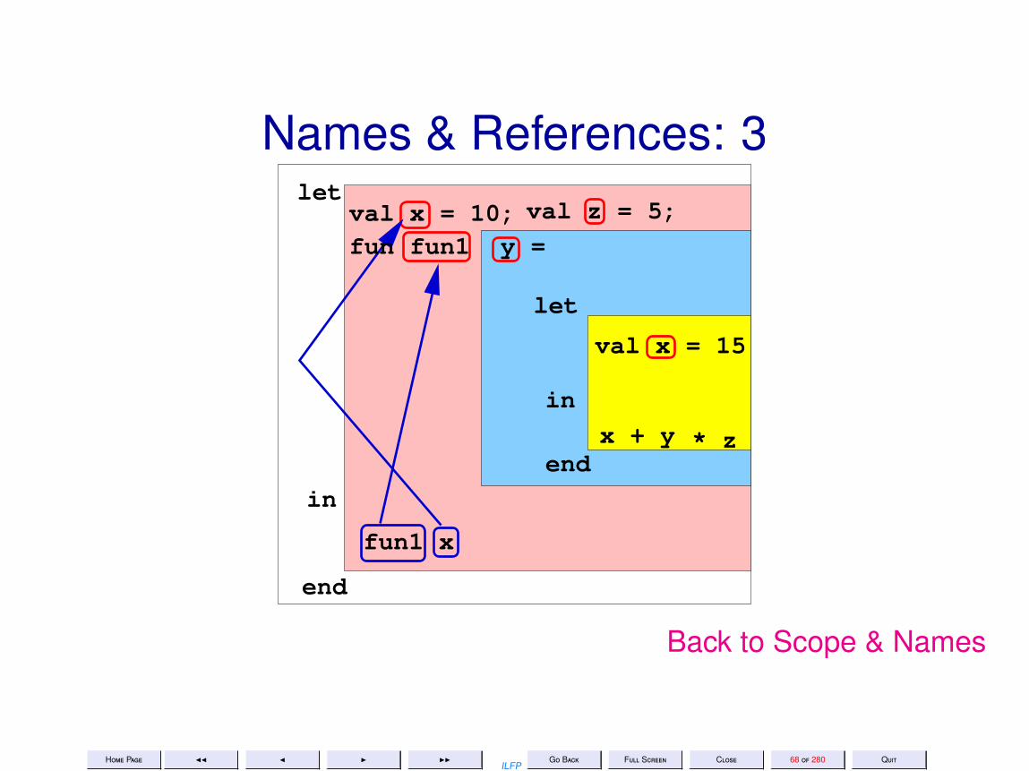
Names & References: 3let
in
end
fun1 x
val x = 10;fun fun1 y =
let
val x = 15
inx + y
end
val z = 5;
* z
Back to Scope & Names
Home Page JJ J I IIILFP
Go Back Full Screen Close 69 of 280 Quit
Names & References: 4let
in
end
fun1 x
val x = 10;fun fun1 y =
let
val x = 15
inx + y
end
val z = 5;
* z
Back to Scope & Names

Home Page JJ J I IIILFP
Go Back Full Screen Close 70 of 280 Quit
Names & References: 5let
in
end
fun1 x
val x = 10;fun fun1 y =
let
val x = 15
inx + y
end
val z = 5;
* z
Back to Scope & Names

Home Page JJ J I IIILFP
Go Back Full Screen Close 71 of 280 Quit
Names & References: 6let
in
end
fun1 x
val x = 10;fun fun1 y =
let
val x = 15
inx + y
end
val z = 5;
* z
Back to Scope & Names

Home Page JJ J I IIILFP
Go Back Full Screen Close 72 of 280 Quit
Names & References: 7let
end
val x = 10;fun fun1 y =
let...
in...
end
fun fun2 z =let ...in ...end
fun1 (fun2 x)
val x = x − 5;
in
Back to Scope & Names

Home Page JJ J I IIILFP
Go Back Full Screen Close 73 of 280 Quit
Names & References: 8let
end
val x = 10;fun fun1 y =
let...
in...
end
fun fun2 z =let ...in ...end
fun1 (fun2 x)
val x = x − 5;
in
Back to Scope & Names

Home Page JJ J I IIILFP
Go Back Full Screen Close 74 of 280 Quit
Names & References: 9let
end
val x = 10;fun fun1 y =
let...
in...
end
fun fun2 z =let ...in ...end
fun1 (fun2 x)
val x = x − 5;
in
Back to Scope & Names

Home Page JJ J I IIILFP
Go Back Full Screen Close 75 of 280 Quit
Definition of NamesDefinitions are of the formqualifier name . . . = body
• val name =• fun name ( argnames ) =
• local de f initionsin de f initionend

Home Page JJ J I IIILFP
Go Back Full Screen Close 76 of 280 Quit
Use of NamesNames are used in expressions.Expressions may occur
• by themselves – to be evaluated• as the body of a definition• as the body of a let-expressionlet de f initionsin expressionend
use of local

Home Page JJ J I IIILFP
Go Back Full Screen Close 77 of 280 Quit
Scope & local
end
localfun fun1 y =
fun fun2 z =
infun fun3 x =
...
fun2 ...fun1 ...
...
...fun1

Home Page JJ J I IIILFP
Go Back Full Screen Close 80 of 280 Quit
6. Lecture 6: Sample Sort Programs
Lecture 6: Sample Sort ProgramsFriday 05 Aug 2011

Home Page JJ J I IIILFP
Go Back Full Screen Close 81 of 280 Quit
6.1. Insertion Sort
Let’s consider the development of a program to sort a list using the insertion sort algorithm, which youmust have all studied before. Notice the use of induction (basis, hypothesis and induction step) inherentin this algorithm.
Problem How do you sort a list of elements by insertion?
For the purpose of development of this algorithm we assume that we are given
input. A list of elements of some unspecified type such that there exists a pre-defined total orderingrelation R on the type of the elements that make up the list.
Our sort function will take this total ordering and the list of elements as parameters.
Strategy. The following cases are to be considered.
Basis. The empty list (and the one-element list) are already sorted.
Induction hypothesis. Assume a list of length m ≥ 0 can be sorted.
Induction step. Given a list of n = m + 1 elements,
1. sort the tail of the list (consisting of n − 1 = m elements). By the induction hypothesis, we knowhow to do this!
2. insert the first element into this sorted list at an appropriate position to obtain a sorted list of length n.
Subproblem How does one insert an element x into a sorted list L of length m ≥ 0 to obtain a sorted listof length m + 1?

Home Page JJ J I IIILFP
Go Back Full Screen Close 82 of 280 Quit
Strategy. The following cases need to be considered.
Basis. If the given sorted list L is empty, then [x] is the resulting sorted list.
Induction hypothesis. Assume it is possible to insert x into a sorted list of length k ≥ 0 to obtain a sortedlist of length k + 1 for k < m.
Induction step. Assume given a sorted list L of length m > 0. Since m > 0, L is non-empty and henceL = h :: t where h is the head of the list and t is the tail. Further t is a list of length m − 1.
1. Compute R(x, h).Case R(x, h) = true. Then x :: L is the required sorted list of length m + 1.Case R(x, h) = f alse. Then insert x into t so as to produce a sorted list t′ of length m (this is possible
by the induction hypothesis). Then h :: t′ is the required sorted list of length m + 1.
Here is the strategy implemented in functional pseudocode.
insertSort R L =
[] if L ∼ []insert R (insertSort R t) h elseif L ∼ h :: t
where
insert R L x =
[x] if L ∼ []x :: L elseif L ∼ h :: t ∧ R(x, h)h :: (insert R t x) else
We use the notation ∼ to indicate “structural pattern-match” rather than equality. Hence in our functioalpseudo-code, “L ∼ h :: t” denotes the statement “L is of the form h :: t where h is the head of the list L and t isthe tail of the list L”. The usual static scope rules for names apply.

Home Page JJ J I IIILFP
Go Back Full Screen Close 83 of 280 Quit
( ∗−−−−−−−−−−−−−−−−−−−−−−−−−−−− INSERTION SORT −−−−−−−−−−−−−−−−−−−−−− ∗ )( ∗ R i s assumed to be a t o t a l ordering r e l a t i o n ∗ )fun i n s e r t S o r t R [ ] = [ ]| i n s e r t S o r t R ( h : : t ) =
l e t fun i n s e r t R [ ] x = [ x ]| i n s e r t R ( h : : t ) x =
i f R ( x , h ) then x : : ( h : : t )e l s e h : : ( i n s e r t R t x )
val r e s t = i n s e r t S o r t R tin i n s e r t R r e s t hend ;
( ∗ Testval i = i n s e r t S o r t ;i ( op <) [ ˜ 1 2 , ˜ 2 4 , ˜ 1 2 , 0 , 123 , 45 , 1 , 20 , 0 , ˜ 2 4 ] ;i ( op <=) [ ˜ 1 2 , ˜ 2 4 , ˜ 1 2 , 0 , 123 , 45 , 1 , 20 , 0 , ˜ 2 4 ] ;i ( op >) [ ˜ 1 2 , ˜ 2 4 , ˜ 1 2 , 0 , 123 , 45 , 1 , 20 , 0 , ˜ 2 4 ] ;i ( op >=) [ ˜ 1 2 , ˜ 2 4 , ˜ 1 2 , 0 , 123 , 45 , 1 , 20 , 0 , ˜ 2 4 ] ;∗ )

Home Page JJ J I IIILFP
Go Back Full Screen Close 84 of 280 Quit
6.2. Selection Sort
Strategy.
Basis. The empty list and the one-element list are already sorted.
Induction hypothesis. Assume a list of length m ≥ 0 can be sorted.
Induction step. Given a list of n > 1 elements,
1. Find and remove the “R-minimal” element from the list of length n > 1.2. Sort the rest of the list (which is of length n − 1).3. Prepend the list with the “R-minimal” element.
selSort R L =
L if L ∼ [] ∨ L ∼ [h]m :: (selSort R M) else
where(m,M) = f indMin R L
where
f indMin R L =
⊥ if L ∼ [](h, []) elseif L ∼ [h](m,L′) elseif L ∼ h :: t
where
(m,L′) =
(m, h :: t′) if (m, t′) = ( f indMin R t) ∧ R(m, h)(h, t) else

Home Page JJ J I IIILFP
Go Back Full Screen Close 85 of 280 Quit
( ∗ −−−−−−−−−−−−−−−−−−−−−−−−−−− SELECTION SORT −−−−−−−−−−−−−−−−−−−−−−−−− ∗ )( ∗ R i s assumed to be a t o t a l ordering r e l a t i o n ∗ )fun s e l S o r t R [ ] = [ ]| s e l S o r t R [ h ] = [ h ]| s e l S o r t R ( L as h : : t ) =
l e t except ion emptyList ;( ∗ findMin f i n d s the minimum element in the l i s t and removes i t ∗ )fun findMin R [ ] = r a i s e emptyList| findMin R [ h ] = ( h , [ ] )| findMin R ( h : : t ) =
l e t val (m, t t ) = findMin R t ;in i f R(m, h ) then (m, h : : t t ) e l s e ( h , t )end ;
val (m, LL ) = findMin R Lin m: : ( s e l S o r t R LL )end ;
( ∗ Testval s = s e l S o r t ;s ( op <) [ ˜ 1 2 , ˜ 2 4 , ˜ 1 2 , 0 , 123 , 45 , 1 , 20 , 0 , ˜ 2 4 ] ;s ( op <=) [ ˜ 1 2 , ˜ 2 4 , ˜ 1 2 , 0 , 123 , 45 , 1 , 20 , 0 , ˜ 2 4 ] ;s ( op >) [ ˜ 1 2 , ˜ 2 4 , ˜ 1 2 , 0 , 123 , 45 , 1 , 20 , 0 , ˜ 2 4 ] ;s ( op >=) [ ˜ 1 2 , ˜ 2 4 , ˜ 1 2 , 0 , 123 , 45 , 1 , 20 , 0 , ˜ 2 4 ] ;∗ )

Home Page JJ J I IIILFP
Go Back Full Screen Close 86 of 280 Quit
( ∗ −−−−−−−−−−−−−−−−−−−−−−−−−−− BUBBLE SORT −−−−−−−−−−−−−−−−−−−−−−−−− ∗ )l o c a l
fun bubble R [ ] = [ ]| bubble R [ h ] = [ h ]| bubble R ( f : : s : : t ) = ( ∗ can ’ t bubble without a t l e a s t 2 elements ∗ )
i f R ( f , s ) then f : : ( bubble R ( s : : t ) )e l s e s : : ( bubble R ( f : : t ) )
fun unsorted R [ ] = f a l s e| unsorted R [ h ] = f a l s e| unsorted R ( f : : s : : t ) =
i f ( f=s ) then ( unsorted R ( s : : t ) )e l s e i f R ( f , s ) then ( unsorted R ( s : : t ) )e l s e t rue
in fun bubbleSort R L =
i f ( unsorted R L ) then ( bubbleSort R ( bubble R L ) )e l s e L
end
( ∗ Testval b = bubbleSort ;b ( op <) [ ˜ 1 2 , ˜ 2 4 , ˜ 1 2 , 0 , 123 , 45 , 1 , 20 , 0 , ˜ 2 4 ] ;b ( op <=) [ ˜ 1 2 , ˜ 2 4 , ˜ 1 2 , 0 , 123 , 45 , 1 , 20 , 0 , ˜ 2 4 ] ;b ( op >) [ ˜ 1 2 , ˜ 2 4 , ˜ 1 2 , 0 , 123 , 45 , 1 , 20 , 0 , ˜ 2 4 ] ;b ( op >=) [ ˜ 1 2 , ˜ 2 4 , ˜ 1 2 , 0 , 123 , 45 , 1 , 20 , 0 , ˜ 2 4 ] ;∗ )

Home Page JJ J I IIILFP
Go Back Full Screen Close 87 of 280 Quit
( ∗ −−−−−−−−−−−−−−−−−−−−−−−− MERGE SORT −−−−−−−−−−−−−−−−−−−−−−−−−−−−−−−−−− ∗ )fun mergeSort R [ ] = [ ]| mergeSort R [ h ] = [ h ]| mergeSort R L = ( ∗ can ’ t s p l i t a l i s t unless i t has > 1 element ∗ )
l e t fun s p l i t [ ] = ( [ ] , [ ] )| s p l i t [ h ] = ( [ h ] , [ ] )| s p l i t ( h1 : : h2 : : t ) =
l e t val ( l e f t , r i g h t ) = s p l i t t ;in ( h1 : : l e f t , h2 : : r i g h t )
end ;val ( l e f t , r i g h t ) = s p l i t L ;fun merge (R , [ ] , [ ] ) = [ ]| merge (R , [ ] , ( L2 as h2 : : t 2 ) ) = L2| merge (R , ( L1 as h1 : : t 1 ) , [ ] ) = L1| merge (R , ( L1 as h1 : : t 1 ) , ( L2 as h2 : : t 2 ) ) =
i f R( h1 , h2 ) then h1 : : ( merge (R , t1 , L2 ) )e l s e h2 : : ( merge (R , L1 , t2 ) ) ;
val s o r t e d L e f t = mergeSort R l e f t ;val sor tedRight = mergeSort R r i g h t ;
in merge (R , sor tedLef t , sor tedRight )end ;

Home Page JJ J I IIILFP
Go Back Full Screen Close 88 of 280 Quit
( ∗ −−−−−−−−−−−−−−−−−−−−−−−−−−−−− QUICK SORT −−−−−−−−−−−−−−−−−−−−−−−−−− ∗ )fun quickSort R [ ] = [ ]| quickSort R ( h : : t ) =
l e t fun part R p [ ] = ( [ ] , [ ] )| part R p ( f : : r ) =
l e t val ( l e s s e r , g r e a t e r ) = part R p rin i f R ( f , p ) then ( f : : l e s s e r , g r e a t e r )
e l s e ( l e s s e r , f : : g r e a t e r )end
val ( l e f t , r i g h t ) = part R h t ;val s o r t e d L e f t = quickSort R l e f t ;val sor tedRight = quickSort R r i g h t ;
in s o r t e d L e f t @ ( h : : sor tedRight )end ;

Home Page JJ J I IIILFP
Go Back Full Screen Close 89 of 280 Quit
( ∗ The l e x i c o g r a p h i c ordering on s t r i n g s ∗ )fun l e x l t ( s , t ) =
l e t val Ls = explode ( s ) ;val Lt = explode ( t ) ;fun l s t l e x l t ( , [ ] ) = f a l s e| l s t l e x l t ( [ ] , ( b : char ) : :M) = t rue| l s t l e x l t ( a : : L , b : :M) =
i f ( a < b ) then truee l s e i f ( a = b ) then l s t l e x l t ( L , M)
e l s e f a l s e;
in l s t l e x l t ( Ls , Lt )end
fun l e x l e q ( s , t ) = ( s = t ) o r e l s e l e x l t ( s , t )
fun l e x g t ( s , t ) = l e x l t ( t , s )
fun lexgeq ( s , t ) = ( s = t ) o r e l s e l e x g t ( s , t )

Home Page JJ J I IIILFP
Go Back Full Screen Close 91 of 280 Quit
7. Lecture 7: Higher-order Functions
Lecture 7: Higher-order FunctionsTuesday 09 Aug 2011

Home Page JJ J I IIILFP
Go Back Full Screen Close 92 of 280 Quit
Functions in SML1. All functions are unary.• Parameterless functions take the empty tuple as argument• Functions with a single parameter take a single 1-tuple as argument.• Functions of m parameters take a single m-tuple as argument.
2. Functions are first-class objects. Any function may be treated as avalue (except when ...). So we can have• functions on data structures and• data structures of functions
Example 7.1 Creating a list of Functions

Home Page JJ J I IIILFP
Go Back Full Screen Close 93 of 280 Quit
Functions: Mathematics & ProgrammingFunctions in programming differ from mathematical functions in at leasttwo fundamental ways.1. There is no notion of function equality in programming
Example 7.2 f actL2(n) ?= factL (n) cannot be checked by a program.
2. Mathematically equivalent definitions are not necessarily program equiv-alent.
Example 7.3
f L(n) =
1 if n ≤ 0f L(n − 1) ∗ n else f L′(n) =
1 if n ≤ 0f L′(n + 1)/(n + 1) else

Home Page JJ J I IIILFP
Go Back Full Screen Close 94 of 280 Quit
ListsAn ′a list L• is an ordered sequence of elements all of the same type ′a,•may be empty (called nil and denoted either by [] or nil).• only the first element (called the head) of the list is immediately acces-
sible through the unary operation hd.• the tail of the list for a nonempty list is the list without the head and is
obtained by the unary operation tl• There is an operation (called cons denoted by the infix operation ::) for
prepending an element of type ′a to a list of type ′a list.• L satisfies the following conditional equation.
L , nil⇒ L = (hd L) :: (tl L) (1)

Home Page JJ J I IIILFP
Go Back Full Screen Close 95 of 280 Quit
A Progression of Functions1. Creating a list of Functions2. Arithmetic Progressions3. Geometric Progressions

Home Page JJ J I IIILFP
Go Back Full Screen Close 96 of 280 Quit
List of Functions: 1Suppose we want a long list of functions to be generated
[incrby1, incrby2, incrby3, . . . , incrby1000]
where the function incrbyk is a unary function that increments a giveninput value by k. Here is one way to generate the list
fun incrby x = fn y => (x+y);
fun listincrby n = if n <= 0 then []else listincrby (n-1)@[(incrby n)]

Home Page JJ J I IIILFP
Go Back Full Screen Close 97 of 280 Quit
List of Functions: 2A more efficient way of doing it would use “::” instead of “@”.
local
fun listincrby_tr (m, k, L) =if k >= m then L
else listincrby_tr (m, k+1, (incrby (m-k))::L)
in fun listincrby’ n =
if n <= 0 then []
else listincrby_tr (n, 0, [])
end
fun applyl [] x = []
| applyl (h::t) x = (h x)::(applyl t x)

Home Page JJ J I IIILFP
Go Back Full Screen Close 98 of 280 Quit
Higher-order Functions on Lists1. map applies a unary function uniformly to all elements of a list and yields
the list of result values.
fun map f [] = []
| map f (h::t) = (f h)::(map f t)
2. foldl applies a binary function to all elements of a list from left to rightstarting from an identity element.
fun foldl f e [] = e
| foldl f e (h::t) = foldl f (f(h, e)) t
3. foldr operates from right to left
fun foldr f e [] = e
| foldl f e (h::t) = f (h, foldr f e t)

Home Page JJ J I IIILFP
Go Back Full Screen Close 99 of 280 Quit
Arithmetic Progressions: 1
AP1(a, d,n) =
[] if n ≤ 0a :: AP1(a + d, d,n − 1) else
Home Page JJ J I IIILFP
Go Back Full Screen Close 100 of 280 Quit
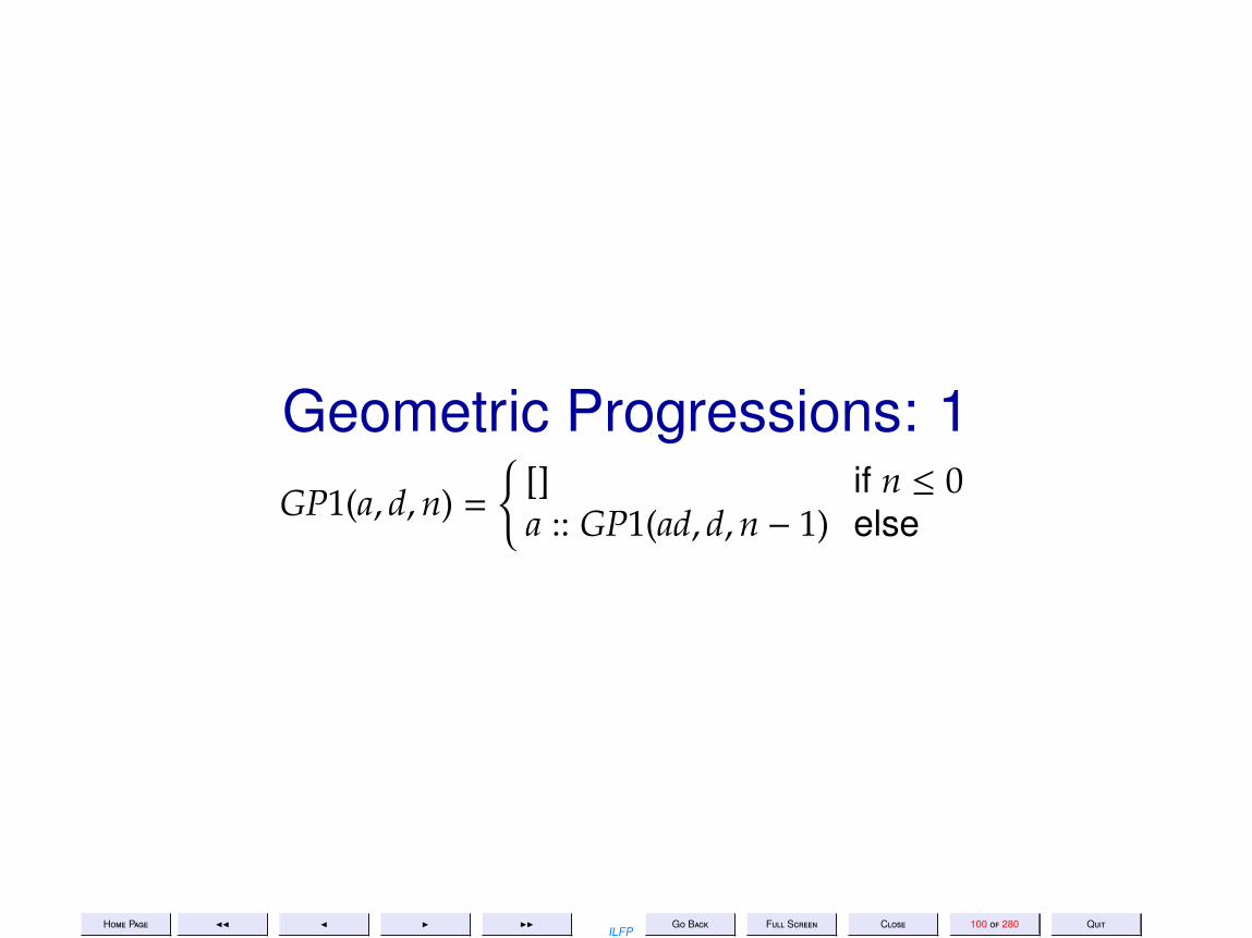
Geometric Progressions: 1GP1(a, d,n) =
[] if n ≤ 0a :: GP1(ad, d,n − 1) else

Home Page JJ J I IIILFP
Go Back Full Screen Close 101 of 280 Quit
Arithmetic-Geometric Progressions: 1AGP1 bop (a, d,n) =
[] if n ≤ 0a :: (AGP1 bop (bop(a, d), d,n − 1)) else

Home Page JJ J I IIILFP
Go Back Full Screen Close 102 of 280 Quit
Arithmetic Progressions: 2
AP2(a, d,n) =
[] if n ≤ 0AP2 tr(a, d,n, []) else
where
AP2 tr(a, d,n,L) =
L if n ≤ 0AP2 tr(a, d,n − 1, (a + d ∗ (n − 1)) :: L) else
Home Page JJ J I IIILFP
Go Back Full Screen Close 103 of 280 Quit
Geometric Progressions: 2
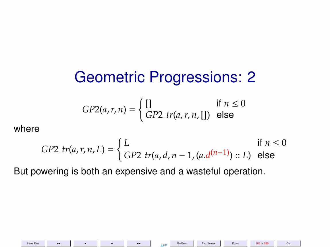
GP2(a, r,n) =
[] if n ≤ 0GP2 tr(a, r,n, []) else
where
GP2 tr(a, r,n,L) =
L if n ≤ 0GP2 tr(a, d,n − 1, (a.d(n−1)) :: L) else
But powering is both an expensive and a wasteful operation.

Home Page JJ J I IIILFP
Go Back Full Screen Close 104 of 280 Quit
More ProgressionsFor any binary operation bop define
curry2 bop = fn x => fn y => bop(x, y)
Then incrby = curry2 op+ and multby = curry2 op*
AP3(a, d,n) =
[] if n ≤ 0a :: (map(curry2 op+ d) AP3(a, d,n − 1)) else
GP3(a, d,n) =
[] if n ≤ 0a :: (map (curry2 op∗ d) AP3(a, d,n − 1)) else
may be generalized to
AGP4 bop (a, d,n) =
[] if n ≤ 0a :: (map (curry2 bop d)(AGP4 bop (a, d,n − 1))) else
AP4 = AGP4 op+GP4 = AGP4 op∗

Home Page JJ J I IIILFP
Go Back Full Screen Close 105 of 280 Quit
Harmonic ProgressionsA harmonic progression is one whose elements are reciprocals of theelements of an arithmetic progression.
HP4(a, d,n) = map reci AP4(a, d,n)
where reci x = 1.0/(real x) for each integer x.We may sum the elements of all the progressions by defining
sumint = f oldl op + 0sumreal = f oldl op + 0.0
AS4(a, d,n) = sumint(AP4(a, d,n))GS4(a, d,n) = sumint(GP4(a, d,n))HS4(a, d,n) = sumreal(HP4(a, d,n))

Home Page JJ J I IIILFP
Go Back Full Screen Close 108 of 280 Quit
8. Lecture 8: Datatypes
Lecture 8: DatatypesWednesday 10 Aug 2011

Home Page JJ J I IIILFP
Go Back Full Screen Close 109 of 280 Quit
Primitive DatatypesThe primitive data types of ML areBooleans: the type bool defined by the structure BoolIntegers: the type int defined by the structure IntReals: the type real defined by the structure Real with a sub-structure
Math of useful constants (e.g. Real.Math.pi) and functions (e.g.Real.Math.sin).
Characters: the type char defined by the structure CharStrings: the type string defined by the structure String

Home Page JJ J I IIILFP
Go Back Full Screen Close 110 of 280 Quit
Structured DataFor any data strucure we require the followingConstructors. which permit the creation and extension of the structure.Destructors or Deconstructors. which permit the breaking up of a struc-
ture into its component parts.Defining Equation. Constructors may be used to reconstruct a data structure
pulled apart by its destructors.
Home Page JJ J I IIILFP
Go Back Full Screen Close 111 of 280 Quit
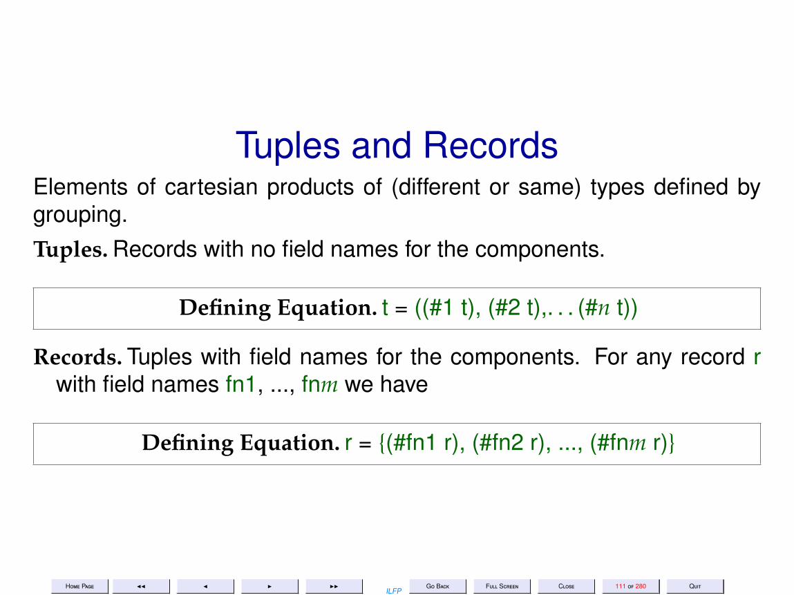
Tuples and RecordsElements of cartesian products of (different or same) types defined bygrouping.Tuples. Records with no field names for the components.
Defining Equation. t = ((#1 t), (#2 t),. . . (#n t))
Records. Tuples with field names for the components. For any record rwith field names fn1, ..., fnm we have
Defining Equation. r = (#fn1 r), (#fn2 r), ..., (#fnm r)

Home Page JJ J I IIILFP
Go Back Full Screen Close 112 of 280 Quit
The List DatatypeA recursively defined datatype conforming to the following ML datatypedefinition
datatype ’ a l i s t = n i l| : : o f ’ a ∗ ’ a l i s t −> ’ a l i s t
i n f i x : :
Constructors. nil and ::Destructors. hd and tl
Defining Equation. L = nil ∨ L = (hd L)::(tl L)

Home Page JJ J I IIILFP
Go Back Full Screen Close 113 of 280 Quit
The Option Datatypedatatype ’ a op t ion = NONE | SOME of ’ a op t ion
Constructors. NONE, SOMEDestructors. valOf
Defining Equation. O = NONE ∨ O = SOME (valOf O)

Home Page JJ J I IIILFP
Go Back Full Screen Close 114 of 280 Quit
The Binary Tree DatatypeA recursive user-defined datatype.
datatype ’ a b i n t r e e = Empty | Node of ’ a ∗ ’ a b i n t r e e ∗ ’ a b i n t r e e
Constructors. Empty, NodeDestructors. root, leftsubtree, rightsubstree
Defining Equation. T = Empty ∨ T = Node (root(T), leftsubtree(T),rightsubtree(T))

Home Page JJ J I IIILFP
Go Back Full Screen Close 115 of 280 Quit
( ∗ The data type binary t r e e ∗ )
datatype ’ a b i n t r e e =
Empty |
Node of ’ a ∗ ’ a b i n t r e e ∗ ’ a b i n t r e e
except ion Empty binary tree
fun isEmpty Empty = t rue| isEmpty = f a l s e
fun subtrees Empty = r a i s e Empty binary tree| subt rees (Node(N, Lst , Rst ) ) = ( Lst , Rst )
fun root Empty = r a i s e Empty binary tree| root (Node(N, , ) ) = N
fun l e f t s u b t r e e Empty = r a i s e Empty binary tree| l e f t s u b t r e e (Node( , Lst , ) ) = Lst
fun r i g h t s u b t r e e Empty = r a i s e Empty binary tree| r i g h t s u b t r e e (Node( , , Rst ) ) = Rst
( ∗ Checking whether a given binary t r e e i s balanced ∗ )

Home Page JJ J I IIILFP
Go Back Full Screen Close 116 of 280 Quit
fun height Empty = 0| height (Node(N, Lst , Rst ) ) =
1+ I n t . max ( height ( Lst ) , height ( Rst ) )
fun isBalanced Empty = t rue| i sBalanced (Node(N, Lst , Rst ) ) =
( abs ( height ( Lst ) − height ( Rst ) ) <= 1) andalsoisBalanced ( Lst ) andalso isBalanced ( Rst )
fun s i z e Empty = 0| s i z e (Node(N, Lst , Rst ) ) = 1+ s i z e ( Lst )+ s i z e ( Rst )
( ∗ Here i s a s i m p l i s t i c d e f i n i t i o n of preorder t r a v e r s a l ∗ )fun preorder1 Empty = n i l| preorder1 (Node(N, Lst , Rst ) ) =
[N] @ preorder1 ( Lst ) @ preorder1 ( Rst )
( ∗ The above d e f i n i t i o n though c o r r e c t i s i n e f f i c i e n t because i t hascomplexity c l o s e r to n ˆ2 s i n c e the append funct ion i t s e l f i s l i n e a r inthe length of the l i s t . We would l i k e an algorithm t h a t i s l i n e a r in thenumber of nodes of the t r e e . So here i s a new one , which uses an i t e r a t i v ea u x i l i a r y funct ion t h a t s t o r e s the preorder t r a v e r s a l of the r i g h t subtreeand then gradual ly a t t a c h e s the preorder t r a v e r s a l of the l e f t subtreeand f i n a l l y a t t a c h e s the root as the head of the l i s t .
∗ )

Home Page JJ J I IIILFP
Go Back Full Screen Close 117 of 280 Quit
l o c a l fun pre ( Empty , L l i s t ) = L l i s t| pre (Node (N, Lst , Rst ) , L l i s t ) =
l e t val Ml is t = pre ( Rst , L l i s t )val N l i s t = pre ( Lst , Ml is t )
in N: : N l i s tend
in fun preorder2 T = pre ( T , [ ] )end
val preorder = preorder2
( ∗ S i m i l a r l y l e t ’ s do inorder and postorder t r a v e r s a l ∗ )fun inorder1 Empty = n i l| inorder1 (Node(N, Lst , Rst ) ) =
inorder1 ( Lst ) @ [N] @ inorder1 ( Rst )
l o c a l fun ino ( Empty , L l i s t ) = L l i s t| ino (Node (N, Lst , Rst ) , L l i s t ) =
l e t val Ml is t = ino ( Rst , L l i s t )val N l i s t = ino ( Lst , N: : Ml is t )
in N l i s tend
in fun inorder2 T = ino ( T , [ ] )end
val inorder = inorder2

Home Page JJ J I IIILFP
Go Back Full Screen Close 118 of 280 Quit
fun postorder1 Empty = n i l| postorder1 (Node (N, Lst , Rst ) ) =
postorder1 ( Lst ) @ postorder1 ( Rst ) @ [N]
l o c a l fun post ( Empty , L l i s t ) = L l i s t| post (Node (N, Lst , Rst ) , L l i s t ) =
l e t val Ml is t = post ( Rst , N: : L l i s t )val N l i s t = post ( Lst , Ml i s t )
in N l i s tend
in fun postorder2 T = post ( T , [ ] )end
val postorder = postorder2
( ∗ A map funct ion f o r binary t r e e s ∗ )
fun BTmap f =
l e t fun BTM Empty = Empty| BTM (Node(N, Lst , Rst ) ) =
Node ( ( f N) , BTM ( Lst ) , BTM ( Rst ) )in BTMend
( ∗ Example i n t e g e r binary t r e e : Notice t h a t 2 has an empty l e f t subtreeand 5 has an empty r i g h t subtree .

Home Page JJ J I IIILFP
Go Back Full Screen Close 119 of 280 Quit
1/ \
/ \
2 3\ / \
4 5 7/
6∗ )val t7 = Node ( 7 , Empty , Empty ) ;val t6 = Node ( 6 , Empty , Empty ) ;val t4 = Node ( 4 , Empty , Empty ) ;val t2 = Node ( 2 , Empty , t4 ) ;val t5 = Node ( 5 , t6 , Empty ) ;val t3 = Node ( 3 , t5 , t 7 ) ;val t1 = Node ( 1 , t2 , t 3 ) ;

Home Page JJ J I IIILFP
Go Back Full Screen Close 121 of 280 Quit
9. Lecture 9: Information Hiding
Lecture 9: Information HidingFriday 12 Aug 2011

Home Page JJ J I IIILFP
Go Back Full Screen Close 122 of 280 Quit
Datatype: Constructors & Destructors1. The Defining Equations require for each data type a relation between
its constructors and destructors.2. The data type completely reveals its structure through the constructors3. Even if there are no destructors defined, the structure could be broken
down using pattern-matching.
1. Information Hiding: Separate Compilation2. Information Hiding: Abstraction

Home Page JJ J I IIILFP
Go Back Full Screen Close 123 of 280 Quit
Information Hiding: Separate CompilationInformation hiding is useful for many reasonsSeparate Compilation. Different modules may be compiled separately
and1. a module is loaded only when required by the user program2. module implementations may be changed, separately compiled and
stored. As long as the interface to the user remains unchanged theuser programs will exhibit no change in behaviour.
3. Many different implementations may be provided for the same pack-age specification, allowing a choice of implementations to the user.
Abstraction.

Home Page JJ J I IIILFP
Go Back Full Screen Close 124 of 280 Quit
Information Hiding: AbstractionInformation hiding is useful for many reasonsSeparate Compilation.Abstraction.
1. Requires that the structure of the underlying data should be hiddenfrom user, so that it can be changed whenever found necessary.
2. Reduces clutter in the user code and user code may be read andunderstood clearly without being distracted by unnecessary detailsthat are not essential for functionality of the user’s code.

Home Page JJ J I IIILFP
Go Back Full Screen Close 125 of 280 Quit
Abstract Data Types1. In a datatype definition the constructors of the data type and the struc-
ture of the data type are revealed.2. It is not necessary to program any destructors because of the availabil-
ity of excellent pattern-matching facilites.3. A datatype may be declared abstract, so that absolutely no informa-
tion about its internal structure is revealed and the only access to itscomponents is through its interface.
4. Without destructor functions available in the interface, no inkling of thecomponents of the structure are made available.
bintree.sml vs. abstype-bintree.sml

Home Page JJ J I IIILFP
Go Back Full Screen Close 126 of 280 Quit
abstype-bintree.sml
( ∗ The a b s t r a c t data type binary t r e e ∗ )
abstype ’ a b i n t r e e =
Empty |
Node of ’ a ∗ ’ a b i n t r e e ∗ ’ a b i n t r e ewith
except ion Empty binary tree
fun mktree0 ( ) = Empty
fun mktrees2 (N, TL , TR) = Node(N, TL , TR ) ;
fun isEmpty Empty = t rue| isEmpty = f a l s e
fun subtrees Empty = r a i s e Empty binary tree| subt rees (Node(N, Lst , Rst ) ) = ( Lst , Rst )
fun root Empty = r a i s e Empty binary tree| root (Node(N, , ) ) = N
fun l e f t s u b t r e e Empty = r a i s e Empty binary tree| l e f t s u b t r e e (Node( , Lst , ) ) = Lst
fun r i g h t s u b t r e e Empty = r a i s e Empty binary tree

Home Page JJ J I IIILFP
Go Back Full Screen Close 127 of 280 Quit
| r i g h t s u b t r e e (Node( , , Rst ) ) = Rst
fun height Empty = 0| height (Node(N, Lst , Rst ) ) =
1+ I n t . max ( height ( Lst ) , height ( Rst ) )
fun isBalanced Empty = t rue| i sBalanced (Node(N, Lst , Rst ) ) =
( abs ( height ( Lst ) − height ( Rst ) ) <= 1) andalsoisBalanced ( Lst ) andalso isBalanced ( Rst )
fun s i z e Empty = 0| s i z e (Node(N, Lst , Rst ) ) = 1+ s i z e ( Lst )+ s i z e ( Rst )
( ∗ Here i s a s i m p l i s t i c d e f i n i t i o n of preorder t r a v e r s a l ∗ )fun preorder1 Empty = n i l| preorder1 (Node(N, Lst , Rst ) ) =
[N] @ preorder1 ( Lst ) @ preorder1 ( Rst )
( ∗ The above d e f i n i t i o n though c o r r e c t i s i n e f f i c i e n t because i t hascomplexity c l o s e r to n ˆ2 s i n c e the append funct ion i t s e l f i s l i n e a r inthe length of the l i s t . We would l i k e an algorithm t h a t i s l i n e a r in thenumber of nodes of the t r e e . So here i s a new one , which uses an i t e r a t i v ea u x i l i a r y funct ion t h a t s t o r e s the preorder t r a v e r s a l of the r i g h t subtreeand then gradual ly a t t a c h e s the preorder t r a v e r s a l of the l e f t subtreeand f i n a l l y a t t a c h e s the root as the head of the l i s t .

Home Page JJ J I IIILFP
Go Back Full Screen Close 128 of 280 Quit
∗ )
l o c a l fun pre ( Empty , L l i s t ) = L l i s t| pre (Node (N, Lst , Rst ) , L l i s t ) =
l e t val Ml is t = pre ( Rst , L l i s t )val N l i s t = pre ( Lst , Ml is t )
in N: : N l i s tend
in fun preorder2 T = pre ( T , [ ] )end
val preorder = preorder2
( ∗ A map funct ion f o r binary t r e e s ∗ )
fun BTmap f =
l e t fun BTM Empty = Empty| BTM (Node(N, Lst , Rst ) ) =
Node ( ( f N) , BTM ( Lst ) , BTM ( Rst ) )in BTMend
end ( ∗ with abstype ∗ )
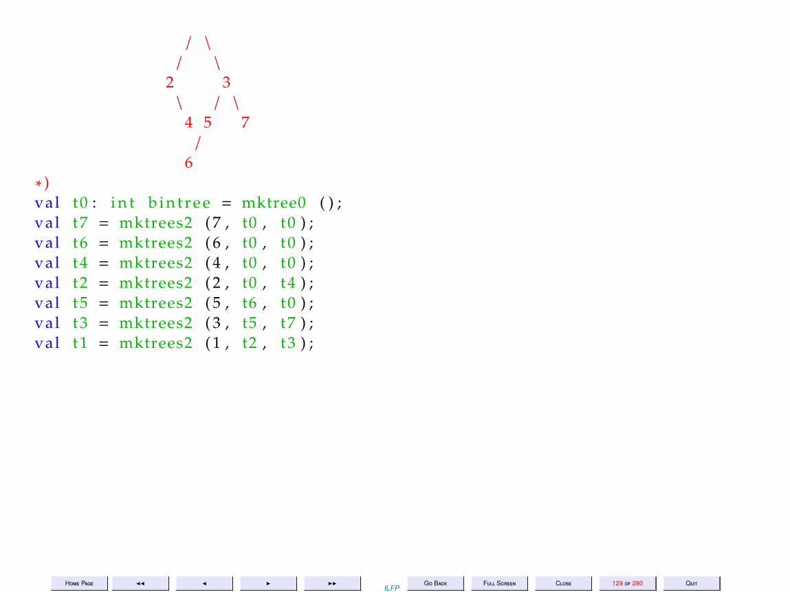
( ∗ Example i n t e g e r binary t r e e : Notice t h a t 2 has an empty l e f t subtreeand 5 has an empty r i g h t subtree .
1
Home Page JJ J I IIILFP
Go Back Full Screen Close 129 of 280 Quit
/ \
/ \
2 3\ / \
4 5 7/
6∗ )val t0 : i n t b i n t r e e = mktree0 ( ) ;val t7 = mktrees2 ( 7 , t0 , t0 ) ;val t6 = mktrees2 ( 6 , t0 , t0 ) ;val t4 = mktrees2 ( 4 , t0 , t0 ) ;val t2 = mktrees2 ( 2 , t0 , t4 ) ;val t5 = mktrees2 ( 5 , t6 , t0 ) ;val t3 = mktrees2 ( 3 , t5 , t7 ) ;val t1 = mktrees2 ( 1 , t2 , t3 ) ;

Home Page JJ J I IIILFP
Go Back Full Screen Close 131 of 280 Quit
10. Lecture 10: Abstract Data Types to Modularity
Lecture 10: Abstract Data Types toModularity
Wednesday 17 Aug 2011
Home Page JJ J I IIILFP
Go Back Full Screen Close 132 of 280 Quit
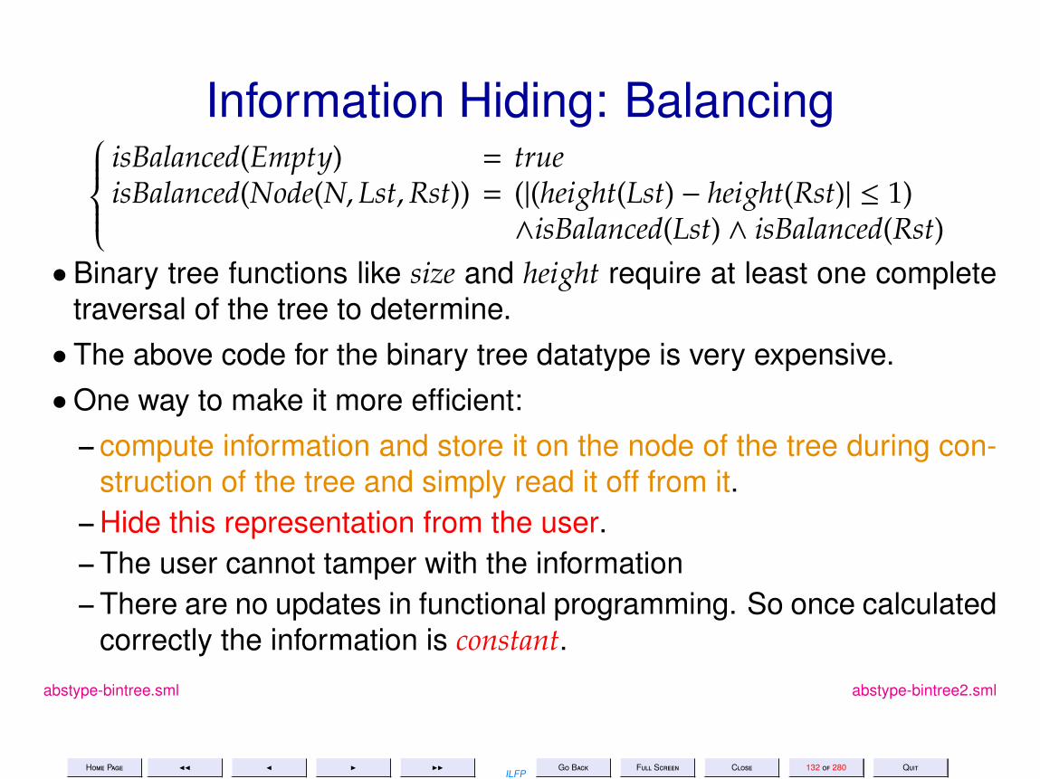
Information Hiding: BalancingisBalanced(Empty) = trueisBalanced(Node(N,Lst,Rst)) = (|(height(Lst) − height(Rst)| ≤ 1)
∧isBalanced(Lst) ∧ isBalanced(Rst)• Binary tree functions like size and height require at least one complete
traversal of the tree to determine.• The above code for the binary tree datatype is very expensive.•One way to make it more efficient:
– compute information and store it on the node of the tree during con-struction of the tree and simply read it off from it.
– Hide this representation from the user.– The user cannot tamper with the information– There are no updates in functional programming. So once calculated
correctly the information is constant.abstype-bintree.sml abstype-bintree2.sml
Home Page JJ J I IIILFP
Go Back Full Screen Close 133 of 280 Quit
abstype-bintree2.sml
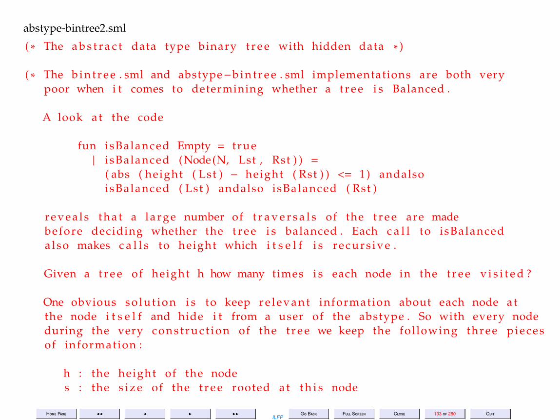
( ∗ The a b s t r a c t data type binary t r e e with hidden data ∗ )
( ∗ The b i n t r e e . sml and abstype−b i n t r e e . sml implementations are both verypoor when i t comes to determining whether a t r e e i s Balanced .
A look at the code
fun isBalanced Empty = t rue| i sBalanced (Node(N, Lst , Rst ) ) =
( abs ( height ( Lst ) − height ( Rst ) ) <= 1) andalsoisBalanced ( Lst ) andalso isBalanced ( Rst )
r e v e a l s t h a t a l a r g e number of t r a v e r s a l s of the t r e e are madebefore deciding whether the t r e e i s balanced . Each c a l l to isBalanceda l s o makes c a l l s to height which i t s e l f i s r e c u r s i v e .
Given a t r e e of height h how many times i s each node in the t r e e v i s i t e d ?
One obvious s o l u t i o n i s to keep r e l e v a n t information about each node atthe node i t s e l f and hide i t from a user of the abstype . So with every nodeduring the very c o n s t r u c t i o n of the t r e e we keep the fol lowing three p i e c e sof information :
h : the height of the nodes : the s i z e of the t r e e rooted at t h i s node

Home Page JJ J I IIILFP
Go Back Full Screen Close 134 of 280 Quit
b : the balance information( height of the l e f t −subtree − height of the r ight −subtree )
i sB : whether the t r e e i s balanced
This information i s hidden from the user and i s used i n t e r n a l l y onlyf o r the height and isBalanced f u n c t i o n s .
The code of the cons t ruc tors , d e s t r u c t o r s and a l l other f u n c t i o n smay have to be changed because of t h i s −− p r e t t y much the e n t i r eimplementation changes with only the names remaining the same .
∗ )
abstype ’ a b i n t r e e 2 =
Empty |
Node of nv : ’ a , h : in t , s : in t , b : in t , i sB : bool ∗’ a b i n t r e e 2 ∗ ’ a b i n t r e e 2
withexcept ion Empty binary tree
fun height Empty = 0| height (Node(N, Lst , Rst ) ) = #h N
fun s i z e Empty = 0| s i z e (Node(N, Lst , Rst ) ) = # s N
fun isBalanced Empty = t rue

Home Page JJ J I IIILFP
Go Back Full Screen Close 135 of 280 Quit
| i sBalanced (Node(N, Lst , Rst ) ) = # isB N
fun mktree0 ( ) = Empty
fun mktrees2 ( n , TL , TR) =
l e t val ( hL , sL , isBL ) = ( height ( TL ) , s i z e ( TL ) , i sBalanced ( TL ) )val (hR , sR , isBR ) = ( height (TR ) , s i z e (TR ) , i sBalanced (TR ) )val b a l i n f o = sL−sR
in Node ( nv = n , h = 1+ I n t . max( hL , hR ) , s=1+sL+sR , b=bal in fo ,i sB =( abs ( b a l i n f o )<=1) andalso isBL andalso isBR , TL , TR)
end
fun isEmpty Empty = t rue| isEmpty = f a l s e
fun subtrees Empty = r a i s e Empty binary tree| subt rees (Node(N, Lst , Rst ) ) = ( Lst , Rst )
fun root Empty = r a i s e Empty binary tree| root (Node(N, , ) ) = #nv N
fun l e f t s u b t r e e Empty = r a i s e Empty binary tree| l e f t s u b t r e e (Node( , Lst , ) ) = Lst
fun r i g h t s u b t r e e Empty = r a i s e Empty binary tree| r i g h t s u b t r e e (Node( , , Rst ) ) = Rst

Home Page JJ J I IIILFP
Go Back Full Screen Close 136 of 280 Quit
( ∗ Here i s a s i m p l i s t i c d e f i n i t i o n of preorder t r a v e r s a l ∗ )fun preorder1 Empty = n i l| preorder1 (Node(N, Lst , Rst ) ) =
[ ( # nv N) ] @ preorder1 ( Lst ) @ preorder1 ( Rst )
( ∗ The above d e f i n i t i o n though c o r r e c t i s i n e f f i c i e n t because i t hascomplexity c l o s e r to n ˆ2 s i n c e the append funct ion i t s e l f i s l i n e a r inthe length of the l i s t . We would l i k e an algorithm t h a t i s l i n e a r in thenumber of nodes of the t r e e . So here i s a new one , which uses an i t e r a t i v ea u x i l i a r y funct ion t h a t s t o r e s the preorder t r a v e r s a l of the r i g h t subtreeand then gradual ly a t t a c h e s the preorder t r a v e r s a l of the l e f t subtreeand f i n a l l y a t t a c h e s the root as the head of the l i s t .
∗ )
l o c a l fun pre ( Empty , L l i s t ) = L l i s t| pre (Node (N, Lst , Rst ) , L l i s t ) =
l e t val Ml is t = pre ( Rst , L l i s t )val N l i s t = pre ( Lst , Ml is t )
in (# nv N ) : : N l i s tend
in fun preorder2 T = pre ( T , [ ] )end

Home Page JJ J I IIILFP
Go Back Full Screen Close 137 of 280 Quit
val preorder = preorder2
( ∗ A map funct ion f o r binary t r e e s ∗ )
fun BTmap f =
l e t fun BTM Empty = Empty| BTM (Node(N, Lst , Rst ) ) =
Node ( nv = f (# nv N) , s= (# s N) , h= (# h N) , b=(#b N) , i sB = (# i sB N) ,BTM ( Lst ) , BTM ( Rst ) )
in BTMend
end ( ∗ with abstype ∗ )

Home Page JJ J I IIILFP
Go Back Full Screen Close 139 of 280 Quit
11. Lecture 11: Signatures, Structures & Functors
Lecture 11: Signatures, Structures &Functors
Friday 19 Aug 2011

Home Page JJ J I IIILFP
Go Back Full Screen Close 140 of 280 Quit
Towards ModularityConsider an abstract data type for which there are not only several dif-ferent implementations but all the implementations are useful simultane-ously.Example 11.1 Floating point arithmetic for 32-bit precision as well as for64-bit.
Example 11.2 Various implementations of data types such as binarytrees, balanced binary trees, binary search trees etc.

Home Page JJ J I IIILFP
Go Back Full Screen Close 141 of 280 Quit
The Module Facility in SMLThe module facility of ML lifts the concepts of type, value and function toa higher level in an analogous fashion
signature ↔ typestructure ↔ valuef unctor ↔ f unction

Home Page JJ J I IIILFP
Go Back Full Screen Close 142 of 280 Quit
Modularity1. Modularity is essential for large programs2. Modularity may be used along with hiding of information to provide
fine-grained visibility required of a package.3. Many different implementations for the same package specification
may be provided at the same time.4. Modularity in ML is essentially algebraically defined5. Each module consists of a signature and a structure6. If a structure is defined without a signature, then ML infers a default
signature for the structure without hiding any data or definitions.7. A signature may be used to define the visibility required of a structure
Home Page JJ J I IIILFP
Go Back Full Screen Close 143 of 280 Quit
qu-sig.sml
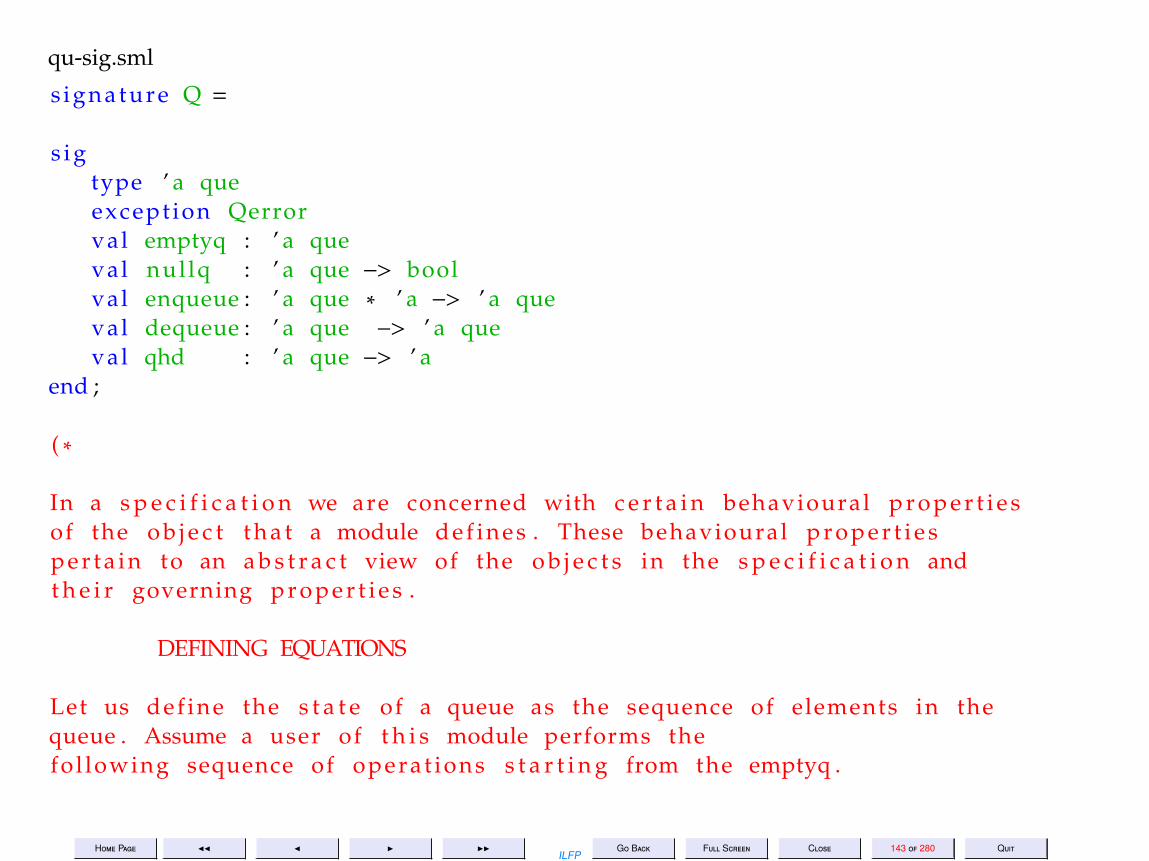
s ignature Q =
s i gtype ’ a queexcept ion Qerrorval emptyq : ’ a queval nul lq : ’ a que −> boolval enqueue : ’ a que ∗ ’ a −> ’ a queval dequeue : ’ a que −> ’ a queval qhd : ’ a que −> ’ a
end ;
( ∗
In a s p e c i f i c a t i o n we are concerned with c e r t a i n behavioural p r o p e r t i e sof the o b j e c t t h a t a module de f ines . These behavioural p r o p e r t i e sp e r t a i n to an a b s t r a c t view of the o b j e c t s in the s p e c i f i c a t i o n andt h e i r governing p r o p e r t i e s .
DEFINING EQUATIONS
Let us def ine the s t a t e of a queue as the sequence of elements in thequeue . Assume a user of t h i s module performs thefol lowing sequence of operat ions s t a r t i n g from the emptyq .

Home Page JJ J I IIILFP
Go Back Full Screen Close 144 of 280 Quit
q0 = emptyq ;q1 = enqueue ( q0 , a1 ) ;q2 = enqueue ( q1 , a2 ) ;q3 = dequeue ( q2 ) ;q4 = enqueue ( q3 , a3 ) ;q5 = dequeue ( q4 ) ;q6 = enqueue ( q5 , a4 ) ;q7 = enqueue ( q6 , a5 ) ;q8 = dequeue ( q7 ) ; ( 1 )
At the end of t h i s sequence of operat ions the queue q8 c o n s i s t s ofthe sequence of elements <a4 , a5> . I f we were to abbrev ia te the”emptyq ” , ”enqueue” and ”dequeue” operat ions r e s p e c t i v e l y by ”<>”,”e” and ”d” , t h i s sequence of operat ions may be regarded as a form ofa l g e b r a i c s i m p l i f i c a t i o n as fo l lows .
d ( e ( e ( d ( e ( d ( e ( e (<> , a1 ) , a2 ) ) , a3 ) ) , a4 ) , a5 ) ) ( 1 )−−−−
= d ( e ( e ( d ( e ( e ( d ( e (<> , a1 ) , a2 ) ) , a3 ) ) , a4 ) , a5 ) ) [ 7 ]−−−−−−−−−−−−
= d ( e ( e ( d ( e ( e (<> , a2 ) ) , a3 ) ) , a4 ) , a5 ) ) [ 6 ]−−−−−
= d ( e ( e ( e ( d ( e (<> , a2 ) ) , a3 ) ) , a4 ) , a5 ) ) [ 7 ]−−−−−−−−−−−−
= d ( e ( e ( e (<> , a3 ) ) , a4 ) , a5 ) ) [ 6 ]

Home Page JJ J I IIILFP
Go Back Full Screen Close 145 of 280 Quit
−−−−
= e ( d ( e ( e (<> , a3 ) ) , a4 ) , a5 ) [ 7 ]−−−−
= e ( e ( d ( e (<> , a3 ) ) , a4 ) , a5 ) [ 7 ]−−−−−−−−−−−−
= e ( e (<> , a4 ) , a5 ) ) [ 6 ]
In other words the sequence of operat ions ( 1 ) may be regarded as beingequiva lent to the sequence ( 2 ) , in terms of the net e f f e c t on thequeue .
q9 = emptyq ;q10 = enqueue ( q9 , a4 ) ;q11 = enqueue ( q10 , a5 ) ( 2 )
At the end of t h i s sequence of operat ions the queue q c o n s i s t s ofthe sequence of elements <a4 , a5> . We may regard t h i s s t a t eas having been obtained by using the equat ions 6 and 7 to reduce thevalue of the queue to a ”normal form” by a l g e b r a i c s i m p l i f i c a t i o n .
The l a s t two equat ions enable us to view the s t a t e of any queue aspossess ing a normal form expressed only in terms of ”emptyq” and asequence of ”enqueue” operat ions on ”emptyq” ( with no occurrence of”dequeue” occurr ing anywhere in the normal form ) .
Any implementation of t h i s s p e c i f i c a t i o n must s a t i s f y the above

Home Page JJ J I IIILFP
Go Back Full Screen Close 146 of 280 Quit
equat ions in order to be considered c o r r e c t . Considering the l e v e lof d e t a i l t h a t there could be in an implementation , t h i s i s o f ten verytedious or cumbersome . However , t h i s seems to be the only way .
DIGRESSION :The notion of a ”normal form” i s very pervasive in mathematics ; f o rexample every polynomial of degree n in one v a r i a b l e x i s wr i t ten as( a ) a sum of terms wri t ten in decreas ing order of t h e i r degrees ,( b ) each term i s a product of a c o e f f i c i e n t and x r a i s e d to a c e r t a i n power ,( c ) no two terms in the r e p r e s e n t a t i o n have the same degree .A l t e r n a t i v e l y one could choose other r e p r e s e n t a t i o n s −− f o r i n s t a n c eas a prodeuct of n f a c t o r s of the form ( x−c i )END OF DIGRESSION∗ )

Home Page JJ J I IIILFP
Go Back Full Screen Close 147 of 280 Quit
Defining Properties/Equations for QFor every q : ′a que and every x : ′a,
0. nullq(emptyq)1. not nullq(enqueue(q, x))2. qhd(emptyq) = Qerror3. qhd(enqueue(q, x)) = x if nullq(q)4. qhd(enqueue(q, x)) = qhd(q) if not(nullq(q))5. dequeue(emptyq) = Qerror6. dequeue(enqueue(q, x)) = emptyq if nullq(q)7. dequeue(enqueue(q, x)) = enqueue(dequeue(q), x) if not(nullq(q))

Home Page JJ J I IIILFP
Go Back Full Screen Close 148 of 280 Quit
11.1. Axiomatic Specifications
We refer to these defining properties/equations as axioms of the queue datatype. These axioms definethe behaviour of the queue datatype in much the same way that the group axioms define the class ofall groups in mathematics and the monoid axioms define the class of all monoids. The class of monoidscontains the class of all groups since every group is a monoid and satisfies all the monoid axioms.
How do these axioms define the “behaviour” of queues? More generally, does every datatype have a setof defining axioms? More particularly, in what way does the behaviour of a queue differ from that of astack?
To answer some of the above questions, we first define the signature and the axioms of the stack datatype.We do this in a manner analogously to what we have defined for queues.
11.1.1. The Stack Datatype
signature S =
sig
type ’a stk
exception Serror
val emptys : ’a stk
val nulls : ’a stk -> bool
val push : ’a stk * ’a -> ’a stk
val pop : ’a stk -> ’a stk
val top : ’a stk -> ’a
end

Home Page JJ J I IIILFP
Go Back Full Screen Close 149 of 280 Quit
Notice that the operations of the stack datatype defined above bear a 1-1 correspondence with theoperations of the queue datatype. The correspondence is shown below.
′a que ↔′a stk
Qerror ↔ Serroremptyq ↔ emptysnullq ↔ nullsenqueue ↔ pushdequeue ↔ popqhd ↔ top
What about the defining equations of the stack datatype? Well here they are and they are indeed analogousto those of the queue. The correspondence in this case is marked by the numbering of the axioms.
For every s : ′a stk and every x : ′a,
0. nulls(emptys)1. not nulls(push(s, x))2. top(emptys) = Serror3. top(push(s, x)) = x
5. pop(emptys) = Serror6. pop(push(s, x)) = s
Notice that even though we have tried to maintain the analogy between queues and stacks, they invariablydo have different axioms and properties. For example the identity 3 in the case of stacks is unconditional
Home Page JJ J I IIILFP
Go Back Full Screen Close 150 of 280 Quit
whereas in the case of queues it requires the corresponding argument q to be empty. Identity 4 in thecase of queues is necessary and conditional, but is entirely redundant in the case of stacks (though theanalogous identity does hold). In a similar manner identity 6 for queues is again conditional but isunconditional in the case of stacks. As in the case 4, identity 7 is redundant for stacks though necessaryfor queues.
One obvious question that arises is, “Are these axioms correct?” That is, are all properties derivable fromthese axioms necessarily true? Another important question is “Are these axioms sufficient to prove allproperties of stacks?” These questions are called soundness and completeness respectively. A third obviousquestion is “How does one think up such axioms?” The answer to this last question is “programmerintuition” and we will leave it at that. A fourth obvious question could be, “If the above axioms are soundand complete, is there a different set of axioms which is also sound and complete?” The answer to thelast question is, “Yes, there could be a different set of sound and complete axioms”.
The signature of the stack defines a collection of all stack expressions which have the type ’a stk forany type ’a of elements. Given a type ’a, notice that the only ways of obtaining objects of the type ’astk are by composing the operations emptys, push and pop. In effect we may define a language of ’astk-expressions (ranged over by the meta-variable se) by the following BNF.
se ::= emptys | push (se, x) | pop (se) (2)
Notice that the BNF (2) allows stack expressions such aspop (emptys), pop (pop (emptys)), push (pop (emptys), x)which do not necessarily yield stacks. The language therefore allows a much larger class of expressionsthan is actually feasible to describe various kinds of stacks.
Our intuition about stacks (a similar analogy holds for queues as well) tells us that the pop operationundoes a push operation, and more importantly any stack expression that is made up of a number ofpush and pop operations equals a stack in which the pop operations and some push operations cancel

Home Page JJ J I IIILFP
Go Back Full Screen Close 151 of 280 Quit
each other resulting in a stack that is either empty or a non-empty stack obtained by a sequence of pusheson an empty stack. We may therefore define a set of standard or normal form of expressions (ranged overby the meta-variable nse) which describes feasible stacks by the following BNF.
nse ::= emptys | push (nse, x) (3)
The BNF (3) reflects the above intuition about stack operations which result in stacks. We call theexpressions generated by BNF (3) normal stack expressions.
Notice first of all that every normal stack expression is also an ’a stk-expressions. Hence the languagegenerated by the BNF (3) is a sub-language of the one generated by the BNF (2). We may also prove thatfollowing lemma.
Lemma 11.3 Every stack expression defined by the BNF (2) which does not yield Serror at any stage, may bereduced to a normal stack expression.
Proof: By induction on the structure of stack expressions. The proof requires the use of the identity 6 toeliminate all occurrences of pop in any stack expression which does not yield Serror. We leave the detailsof the proof to the interested reader. QED
Notice that the normal form is unique.
Lemma 11.4 Every stack expression defined by the BNF (2) which does not yield Serror at any stage, may bereduced to a unique normal stack expression.

Home Page JJ J I IIILFP
Go Back Full Screen Close 152 of 280 Quit
qu1-str.sml
s t r u c t u r e Q1 :Q =
s t r u c t
type ’ a que = ’ a l i s t ;
except ion Qerror ;
val emptyq = [ ] ;
fun nul lq ( [ ] ) = t rue| nul lq ( : : ) = f a l s e;
fun enqueue ( q , x ) = q @ [ x ] ;
( ∗ enqueue takes time l i n e a r in the length of q ∗ )
fun dequeue ( x : : q ) = q| dequeue [ ] = r a i s e Qerror;
fun qhd ( x : : q ) = x| qhd [ ] = r a i s e Qerror;

Home Page JJ J I IIILFP
Go Back Full Screen Close 153 of 280 Quit
( ∗ dequeue and qhd are constant time operat ions ∗ )
end ;
( ∗
Note t h a t the ( pre−defined ) l i s t data type has the fol lowing operat ions :
[ ] −− denotes the empty l i s t ( a l s o c a l l e d ” n i l ” ) .n u l l −− determines whether a l i s t i s empty .: : −− denotes the operat ion ” cons ” which prepends a l i s t with
an element to y i e l d a new l i s t .@ −− denotes the operat ion of ”append”− ing one l i s t to another .hd −− which y i e l d s the f i r s t element of a non−empty l i s tt l −− which y i e l d s the r e s t of the l i s t except i t s head .
Clear ly hd and t l are defined only f o r non−empty l i s t s .
The l i s t data type in turn has a normal form e x p r e s s i b l e only in termsof ” n i l ” and the ” cons ” operat ions . Every l i s t L s a t i s f i e s thefol lowing DATA INVARIANT
0 . L = [ ] or L = hd ( L ) : : t l ( L )
The append operat ion s a t i s f i e s the fol lowing p r o p e r t i e s f o r a l l l i s t s

Home Page JJ J I IIILFP
Go Back Full Screen Close 154 of 280 Quit
L , M.
1 . [ ] @ M = M2 . ( h : : t ) @ M = h : : ( t @ M)
There i s of course another property of append viz .
3 . L @ [ ] = L
But t h i s property can be shown from p r o p e r t i e s 1 . and 2 . by induct ionon the length of the l i s t L .
∗ )

Home Page JJ J I IIILFP
Go Back Full Screen Close 155 of 280 Quit
qu2-str.sml
s t r u c t u r e Q2 :Q =
s t r u c tdatatype ’ a que = emptyq | enqueue of ’ a que ∗ ’ aexcept ion Qerror ;
( ∗ enqueue i s a constant time operat ion ∗ )
fun nul lq emptyq = t rue| nul lq = f a l s e
fun qhd emptyq = r a i s e Qerror| qhd ( enqueue ( emptyq , h ) ) = h| qhd ( enqueue ( q , l ) ) = qhd ( q )
fun dequeue emptyq = r a i s e Qerror| dequeue ( enqueue ( emptyq , h ) ) = emptyq| dequeue ( enqueue ( q , l ) ) = enqueue ( dequeue q , l )
( ∗ dequeue i s l i n e a r in the length of q ∗ )end

Home Page JJ J I IIILFP
Go Back Full Screen Close 156 of 280 Quit
qu3-str.sml
s t r u c t u r e Q3 :Q =
s t r u c t
datatype ’ a que = Queue of ( ’ a l i s t ∗ ’ a l i s t )
val emptyq = Queue ( [ ] , [ ] )
fun nul lq ( Queue ( [ ] , [ ] ) ) = t rue| nul lq ( ) = f a l s e
fun reverse ( L ) =
l e t fun rev ( [ ] , M) = M| rev ( x : : xs , M) = rev ( xs , x : :M)
inrev ( L , [ ] )end
;
fun norm ( Queue ( [ ] , t a i l s ) ) = Queue ( reverse ( t a i l s ) , [ ] )| norm ( q ) = q;

Home Page JJ J I IIILFP
Go Back Full Screen Close 157 of 280 Quit
fun enqueue ( Queue ( heads , t a i l s ) , x ) = norm ( Queue ( heads , x : : t a i l s ) ) ;
except ion Qerror ;
fun dequeue ( Queue ( x : : heads , t a i l s ) ) = norm ( Queue ( heads , t a i l s ) )| dequeue ( Queue ( [ ] , ) ) = r a i s e Qerror;
fun qhd ( Queue ( x : : heads , t a i l s ) ) = x| qhd ( Queue ( [ ] , ) ) = r a i s e Qerror;
( ∗ Clear ly the amortized c o s t of enqueue−ing and dequeue−ing i s l e s s thanl i n e a r in t h i s r e p r e s e n t a t i o n ”most of the time ” .
∗ )
end ;
( ∗This example shows a p e c u l i a r r e p r e s e n t a t i o n of queues and the conceptof information hiding . The funct ion ”norm” i s s p e c i a l to t h i sp a r t i c u l a r r e p r e s e n t a t i o n and t h e r e f o r e should not be v i s i b l e to theuser of the queue . I f t h i s implementation i s c o r r e c t and s a t i s f i e s a l lthe p r o p e r t i e s of the s p e c i f i c a t i o n then one could userepresenta t ion −hiding and the hiding of purely representa t ion −dependentoperat ions l i k e norm to switch between the two implementations without
Home Page JJ J I IIILFP
Go Back Full Screen Close 158 of 280 Quit
a f f e c t i n g any user of t h i s module .
Any user of the Queue module only r e q u i r e s to know the s p e c i f i c a t i o nand use only those funct ions , procedures and operat ions which arev i s i b l e via the s p e c i f i c a t i o n . She would have no use f o r e i t h e r i s s u e st h a t properly p e r t a i n to r e p r e s e n t a t i o n nor with i s s u e s concerning theimplementation of the algori thms in the module .
∗ )

Home Page JJ J I IIILFP
Go Back Full Screen Close 159 of 280 Quit
Exercise 11.1
1. Run through the implementation for the example sequence given in qu-sig.sml given in the specification andsatisfy yourself that this implementation is indeed correct.
2. Prove that each operation on queues in each of the structures correctly implements the specification.
3. Suppose we defined the notion of queues bounded by a certain size, say n. In what way are the behaviouralproperties of such queues different from those of the the unbounded queues defined here?
4. Give a complete set of DATA INVARIANT properties for bounded size queues.

Home Page JJ J I IIILFP
Go Back Full Screen Close 160 of 280 Quit
Signatures1. A signature (c.f. type) specifies the interface to one or more structures
(c.f. values).2. The different implementations of structures Q1, Q2 and Q3 all imple-
ment a common signature.3. Structures may be constrained to signatures by mapping the names of
structures to the names of signatures.(a) the names of the types should match(b) the names of functions and values should also match

Home Page JJ J I IIILFP
Go Back Full Screen Close 161 of 280 Quit
qu-sig-str.sml
use "qu1-str.sml" ;use "qu2-str.sml" ;use "qu3-str.sml" ;use "qu-sig.sml" ;
( ∗ Ins tead i f dec lar ing ”Q1 :Q” , ”Q2 :Q” and ”Q3 :Q” which bind the s t r u c t u r e sto the given s ignature ”Q” , within the s t r u c t u r e one could have l e f t thes t r u c t u r e name unqual i f i ed and l a t e r bound i t as fo l lows
∗ )
( ∗ Transparent Cons t ra in t s −− a l l f u n c t i o n s / data not present in thes ignature are hidden .
∗ )s t r u c t u r e Q1conc : Q = Q1 ;s t r u c t u r e Q2conc : Q = Q2 ;s t r u c t u r e Q3conc : Q = Q3 ; ( ∗ norm i s a hidden funct ion ∗ )
( ∗ Opaque Cons t ra in t s −− underlying r e p r e s e n t a t i o n i s a l s o hidden ∗ )s t r u c t u r e Q1abs :> Q = Q1 ;s t r u c t u r e Q2abs :> Q = Q2 ;s t r u c t u r e Q3abs :> Q = Q3 ;
( ∗ Try the fol lowing and see the d i f f e r e n c e ∗ )open Q3conc ;open Q3abs ;

Home Page JJ J I IIILFP
Go Back Full Screen Close 162 of 280 Quit
11.2. Closing Equational Specifications
One of the problems with the BNF (2) is that it permitted the construction of stack expressions whichwould have yielded the exception Serror. As a result we had to state the lemma 11.3 in such a way thatreduction to the unique normal form BNF (3) was guaranteed only for stack expressions which did not atat any stage raise the exception Serror.
The problems with this formulation are many as noted below:
1. (Unique) normal forms are guaranteed only for a subset of stack expressions, thus leaving out a largenumber syntactically valid expressions to be essentially undefined.
2. The formulation is not very pleasing because it is not general enough.
3. An exception is different from stack expression een theoretically.
A more algebraically elegant formulation which addresses the above problems could be obtained bytaking inspiration from the implementation in “qu2-str.sml” wherein a datatype was defined with emptyqand enqueue being the constructors of the datatype and dequeue is defined as a function which cancelsout appropriate occurrences of the enqueue constructor. An analogous implementation for stacks wouldhave had the following datatype definition
datatype ’a stk = emptys | push of ’a stk * ’a
and of course a corresponding function definition for the pop operation. Notice that this datatypedefinition is really no different from the language of normal stack expressions.
But now what we could do is we could simply eliminate the exception Serror and instead include a 0-ary

Home Page JJ J I IIILFP
Go Back Full Screen Close 163 of 280 Quit
constructor serr in the data-type definition to represent an “error stack”. This has the advantage we couldclose the language of stack expressions so that now every stack expression would not just be syntacticallyvalid, it would also be well-defined.
We thus define the language of extended stack expressions (ranged over by the meta-variable xse) by thefollowing BNF
xse ::= emptys | serr| push (xse, x)| pop(xse) (4)
How does the constructor serr differ in behaviour and properties from the constructor emptys. Verysimply put, every stack operation like push or pop when applied to serr would yield serr. And ofcourse any pop operation on emptys would also yield serr. We may now present a richer and morecomprehensive set of equations and properties for this new type of stack. But before that we need toevaluate the other consequences of what we are doing now.
1. By changing the exception to a valid stack expression we even obtain a different signature. We call thenew signature S’.
2. The functions top and nulls when applied to serr should still yield an exception. Alernatively wecould change the results of applications of these functions to yield an option data type. To reflect thesechanges we call these functions top’ and nulls’ respectively.

Home Page JJ J I IIILFP
Go Back Full Screen Close 164 of 280 Quit
signature S’ =
sig
type ’a stk
val emptys : ’a stk
val serr : ’a stk
val nulls’ : ’a stk -> bool option
val push : ’a stk * ’a -> ’a stk
val pop : ’a stk -> ’a stk
val top’ : ’a stk -> ’a option
end
Returning to the elegance of dealing with serr as just another stack expression we have the followingproperties and equational identities.

Home Page JJ J I IIILFP
Go Back Full Screen Close 165 of 280 Quit
For every s : ′a stk and every x : ′a,
0. nulls′(emptys) = true0′. nulls′(serr) = NONE1. nulls′(push(s, x)) = f alse if s , serr2. top(emptys) = NONE2′. top(serr) = NONE3. top(push(s, x)) = SOME x
5′. pop(emptys) = serr5′′. pop(serr) = serr6. pop(push(s, x)) = s6′. push(serr, x) = serr

Home Page JJ J I IIILFP
Go Back Full Screen Close 166 of 280 Quit
With these equations we also have a language of extended normal form expressions defined as followsand ranged over by the meta-variable nxse.
nxse ::= emptys | serr| push (nxse, x) (5)
We now have the following lemmata (compare these with lemma 11.3 and lemma lem-unique-normal-form respectively).
Lemma 11.5 Every stack expression defined by the BNF (4) may be reduced to a normal stack expression.
Lemma 11.6 Every stack expression defined by the BNF (4) may be reduced to a unique extended normal stackexpression.
As we stated before by making these changes we have changed the signature of the module and all aspectsof the data type. An analogous change may be made int he signature and structure of queues too.

Home Page JJ J I IIILFP
Go Back Full Screen Close 167 of 280 Quit
qu2’-sig-str-sml
( ∗ In t h i s s ignature and s t r u c t u r e we r e p l a c e the except ion Qerror by aa 0−ary c o n s t r u c t o r qerr . This al lows a l l ’ a que−express ions to be c losedunder the queue operat ions . Hence we have the fol lowing e x t r ai d e n t i t i e s on queues
dequeue ( emptyq ) = qerrenqueue ( qerr , x ) = qerrdequeue ( qerr ) = qerr
But i t r a i s e s the a d d i t i o n a l quest ion of what to do about operat ions nul lqand qhd which are supposed to y i e l d r e s p e c t i v e l y a boolean value and an’ a value ?
The obvious answer to these quest ions i s to e i t h e r def ine some other newexcept ions or use the option datatype . We t r y using the option datatype
∗ )
s ignature Q’ =
s i gtype ’ a que( ∗ except ion Qerror ∗ )val qerr : ’ a queval emptyq : ’ a que

Home Page JJ J I IIILFP
Go Back Full Screen Close 168 of 280 Quit
val nullq ’ : ’ a que −> bool optionval enqueue : ’ a que ∗ ’ a −> ’ a queval dequeue : ’ a que −> ’ a queval qhd ’ : ’ a que −> ’ a option
end ;
s t r u c t u r e Q2 ’ : Q’ =
s t r u c tdatatype ’ a que = emptyq | qerr | enq of ’ a que ∗ ’ a( ∗ except ion Qerror ; ∗ )
( ∗ enqueue i s a constant time operat ion ∗ )
fun nullq ’ emptyq = SOME true| nullq ’ qerr = NONE| nullq ’ = SOME f a l s e
fun qhd ’ emptyq = NONE| qhd ’ qerr = NONE| qhd ’ ( enq ( emptyq , h ) ) = SOME h| qhd ’ ( enq ( q , l ) ) = qhd ’ ( q )
fun normalise emptyq = emptyq| normalise qerr = qerr| normalise ( enq ( emptyq , l ) ) = enq ( emptyq , l )| normalise ( enq ( qerr , ) ) = qerr

Home Page JJ J I IIILFP
Go Back Full Screen Close 169 of 280 Quit
| normalise ( enq ( q , l ) ) = ( ∗ enqueue ( normalise q , l ) ) ∗ )l e t val nq = normalise qin case nq of
emptyq => enq ( nq , l )| qerr => qerr| enq ( , ) => enq ( nq , l )
end
fun enqueue ( emptyq , l ) = enq ( emptyq , l )| enqueue ( qerr , ) = qerr| enqueue ( q , l ) = normalise ( enq ( q , l ) )
fun dequeue emptyq = qerr| dequeue qerr = qerr| dequeue ( enq ( emptyq , h ) ) = emptyq| dequeue ( enq ( q , l ) ) = enq ( ( dequeue q ) , l )
( ∗ dequeue i s l i n e a r in the length of q ∗ )end
( ∗ t e s t i n g ∗ )
open Q2 ’ ;
val e = enqueue ;

Home Page JJ J I IIILFP
Go Back Full Screen Close 170 of 280 Quit
val d = dequeue ;
val q1 = e ( d ( emptyq ) , 1 )
val q7 = e ( e ( d ( e ( d ( e ( e ( emptyq , 1 ) , 2 ) ) , 3 ) ) , 4 ) , 5 )
val h7 = valOf ( qhd ’ q7 )
val q8 = d ( e ( e ( d ( e ( d ( e ( e ( emptyq , 1 ) , 2 ) ) , 3 ) ) , 4 ) , 5 ) )
val h8 = qhd ’ q8
val q9 = d ( e ( e ( d ( e ( d ( e ( e ( d ( emptyq ) , 1 ) , 2 ) ) , 3 ) ) , 4 ) , 5 ) )
val h9 = qhd ’ q9
val q10 = d ( e ( e ( d ( e ( d ( e ( d ( d ( e ( emptyq , 1 ) ) ) , 2 ) ) , 3 ) ) , 4 ) , 5 ) )
val h10 = qhd ’ q10

Home Page JJ J I IIILFP
Go Back Full Screen Close 171 of 280 Quit
FunctorsA functor is a structure that takes other structures as parameters andyields a new structure
1. A functor can be applied to argument structures to yield a new structure2. A functor can be applied only to structures that match certain signature
constraints.3. Functors may be used to test existing structures or to create new struc-
tures.4. Functors may also be used to express generic algorithms
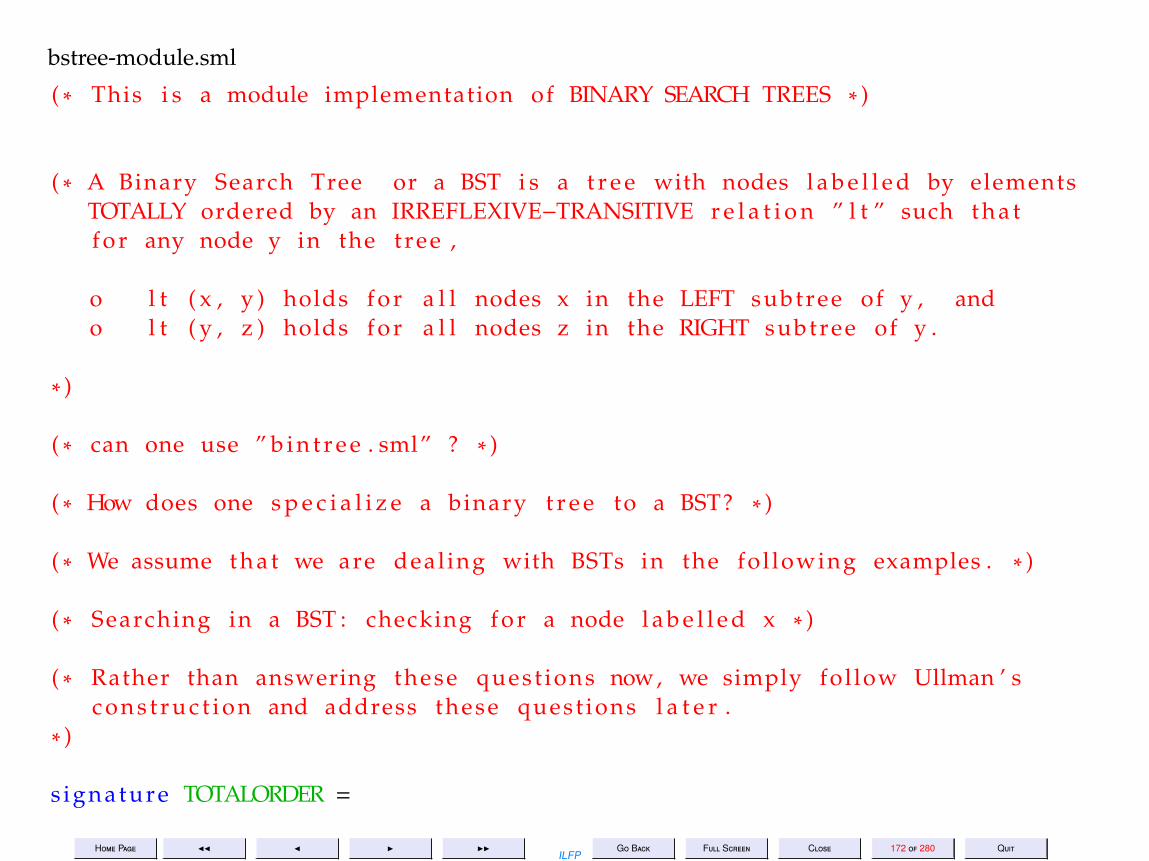
Home Page JJ J I IIILFP
Go Back Full Screen Close 172 of 280 Quit
bstree-module.sml
( ∗ This i s a module implementation of BINARY SEARCH TREES ∗ )
( ∗ A Binary Search Tree or a BST i s a t r e e with nodes l a b e l l e d by elementsTOTALLY ordered by an IRREFLEXIVE−TRANSITIVE r e l a t i o n ” l t ” such t h a tf o r any node y in the tree ,
o l t ( x , y ) holds f o r a l l nodes x in the LEFT subtree of y , ando l t ( y , z ) holds f o r a l l nodes z in the RIGHT subtree of y .
∗ )
( ∗ can one use ” b i n t r e e . sml” ? ∗ )
( ∗ How does one s p e c i a l i z e a binary t r e e to a BST? ∗ )
( ∗ We assume t h a t we are deal ing with BSTs in the fol lowing examples . ∗ )
( ∗ Searching in a BST : checking f o r a node l a b e l l e d x ∗ )
( ∗ Rather than answering these quest ions now, we simply fol low Ullman ’ sc o n s t r u c t i o n and address these quest ions l a t e r .
∗ )
s ignature TOTALORDER =

Home Page JJ J I IIILFP
Go Back Full Screen Close 173 of 280 Quit
s i geqtype e l typeval l t : e l type ∗ e l type −> bool
end ( ∗ s i g ∗ ) ;
s t r u c t u r e INTLAB : TOTALORDER =
s t r u c ttype e l type = i n t ;val l t = op<
end ;
s t r u c t u r e STRINGLAB : TOTALORDER =
s t r u c t
type e l type = s t r i n g ;( ∗ Lexicographic ordering ’< ’ on s t r i n g s ∗ )
fun l e x l t ( s , t ) =
l e t val Ls = explode ( s ) ;val Lt = explode ( t ) ;fun l s t l e x l t ( , [ ] ) = f a l s e| l s t l e x l t ( [ ] , ( b : char ) : :M) = t rue| l s t l e x l t ( a : : L , b : :M) =
i f ( a < b ) then truee l s e i f ( a = b ) then l s t l e x l t ( L , M)

Home Page JJ J I IIILFP
Go Back Full Screen Close 174 of 280 Quit
e l s e f a l s e;
in l s t l e x l t ( Ls , Lt )end
;
val l t = l e x l t ;
end ( ∗ s t r u c t ∗ ) ;
func tor MakeBST ( Lt : TOTALORDER) :s i g
( ∗ open Lt ; ∗ )
( ∗ The use of t h i s ”open” i s an e r r o r in Ullman ’ s book . At l e a s t i t does notseem to be allowed in vers ion 1 0 9 . 3 2 . We have ins tead replaced a l l occurrencesof ” e l type ” in the s ignature by ” Lt . e l type ” and then i t seems to work f i n e .∗ )
type ’ a b i n t r e e ;except ion Empty tree ;val c r e a t e : Lt . e l type b i n t r e e ;val lookup : Lt . e l type ∗ Lt . e l type b i n t r e e −> bool ;val i n s e r t : Lt . e l type ∗ Lt . e l type b i n t r e e −> Lt . e l type b i n t r e e ;val deletemin : Lt . e l type b i n t r e e −> Lt . e l type ∗ Lt . e l type b i n t r e e ;val d e l e t e : Lt . e l type ∗ Lt . e l type b i n t r e e −> Lt . e l type b i n t r e e

Home Page JJ J I IIILFP
Go Back Full Screen Close 175 of 280 Quit
end=
s t r u c topen Lt ;datatype ’ a b i n t r e e =
Empty |
Node of ’ a ∗ ’ a b i n t r e e ∗ ’ a b i n t r e e;
val c r e a t e = Empty ;
fun lookup ( x , Empty ) = f a l s e| lookup ( x , Node ( y , l e f t , r i g h t ) ) =
i f x=y then truee l s e i f l t ( x , y ) then lookup ( x , l e f t )e l s e lookup ( x , r i g h t )
;
( ∗ I n s e r t an element i n t o a BST ∗ )
fun i n s e r t ( x , Empty ) = Node ( x , Empty , Empty )| i n s e r t ( x , T as Node ( y , l e f t , r i g h t ) ) =
i f x=y then T ( ∗ do nothing ∗ )e l s e i f l t ( x , y ) then Node ( y , i n s e r t ( x , l e f t ) , r i g h t )e l s e Node ( y , l e f t , i n s e r t ( x , r i g h t ) )
;

Home Page JJ J I IIILFP
Go Back Full Screen Close 176 of 280 Quit
( ∗ Delete ( i f i t i s there ) from a BST ∗ )
( ∗ Delet ion r e q u i r e s the fol lowing funct ion which can d e l e t e thes m a l l e s t element from a t r e e ; Note t h a t the s m a l l e s t element in aBST i s the l e f t m o s t l e a f −node in the t r e e ( i f i t e x i s t s , otherwisethe root ) . The funct ion deletemin should a l s o re turn the value of thes m a l l e s t element to enable t r e e reorder ing f o r d e l e t i o n .
∗ )
except ion Empty tree ;
fun deletemin ( Empty ) = r a i s e Empty tree| deletemin (Node ( y , Empty , r i g h t ) ) = ( y , r i g h t )| deletemin (Node ( y , l e f t , r i g h t ) ) =
l e t val ( z , L ) = deletemin ( l e f t )in ( z , Node ( y , L , r i g h t ) )end
;
( ∗ NOTE t h a t deletemin does not requi re the comparison funct ion l t as aparameter .
∗ )
fun d e l e t e ( x , Empty ) = Empty| d e l e t e ( x , Node ( y , l e f t , r i g h t ) ) =

Home Page JJ J I IIILFP
Go Back Full Screen Close 177 of 280 Quit
i f x=y theni f l e f t = Empty then r i g h te l s e i f r i g h t = Empty then l e f te l s e ( ∗ e x t r a c t the s m a l l e s t element from the r i g h t subtree
and make i t the root of the new t r e e∗ )l e t val ( z , R) = deletemin ( r i g h t )in Node ( z , l e f t , R)end
e l s e i f l t ( x , y ) then Node ( y , d e l e t e ( x , l e f t ) , r i g h t )e l s e Node ( y , l e f t , d e l e t e ( x , r i g h t ) )
;
end ( ∗ s t r u c t ∗ ) ;
( ∗ Now we may apply the functor MakeBST to STRINGLAB to obta in a new s t r u c t u r eStringBST which def ines ” binary search t r e e s l a b e l l e d by s t r i n g s ordered bythe l e x i c o g r a p h i c t o t a l ordering .
∗ )
s t r u c t u r e StringBST = MakeBST (STRINGLAB ) ; ( ∗ applying the functor ∗ )
s t r u c t u r e IntBST = MakeBST (INTLAB ) ;

Home Page JJ J I IIILFP
Go Back Full Screen Close 179 of 280 Quit
12. Lecture 12: Example: Tautology Checking
Lecture 12: Example: Tautology CheckingTuesday 23 Aug 2011

Home Page JJ J I IIILFP
Go Back Full Screen Close 180 of 280 Quit
ArgumentsA typical informally stated argument might go as follows:If prices rise, then the poor and the salaried class will be unhappy.
If taxes are increased then the businessmen will be unhappy.
If the poor and the salaried class or the businessmen are unhappy, the Government will not be re-elected.
Inflation will rise if Government expenditure exceeds its revenue.
Government expenditure will exceed its revenue unless taxes are increased or the Government resorts to deficit
financing or takes a loan from the IMF to cover the deficit.
If the Government resorts to deficit financing then inflation will rise.
If inflation rises, the prices will also rise.
The Government will get reelected.
Therefore the Government will take a loan from the IMF.

Home Page JJ J I IIILFP
Go Back Full Screen Close 181 of 280 Quit
Arguments: 2A typical informally stated argument might go as follows:If prices rise, then the poor and the salaried class will be unhappy.
If taxes are increased then the businessmen will be unhappy.
If the poor and the salaried class are unhappy or the businessmen are unhappy,
the Government will not be re-elected.
Inflation will rise if Government expenditure exceeds its revenue.
Government expenditure will exceed its revenue unless taxes are increased or
the Government resorts to deficit financing or takes a loan from the IMF to cover the deficit.
If the Government resorts to deficit financing then inflation will rise.
If inflation rises, the prices will also rise.
The Government will get reelected.
Therefore the Government will take a loan from the IMF.

Home Page JJ J I IIILFP
Go Back Full Screen Close 182 of 280 Quit
Arguments in natural language
It turns out that the correctness or otherwise of most arguments depends entirely on the “shapes” ofthe formulae concerned rather than their intrinsic meaning. Take the previous argument. Suppose weuniformly replace the various atoms by say sentences from nursery rhymes as the following table shows:
Prices rise Mary has a little lambThe poor and . . . Little Bo-Peep loses her sheepTaxes are increased Jack and Jill go up the hillThe businessmen will be unhappy Humpty-Dumpty sits on the wallThe Government will get re-elected I am little teapotInflation will rise Little Jack Horner sits in a cornerGovernment expenditure . . . revenue The boy stands on the burning deckThe Government resorts . . . Wee Willie Winkie runs through the townThe Government takes a loan . . . deficit Eensy Weensy spider climbs up the water spout
Then we get the following ridiculous sounding argument
If Mary has a little lamb, then Little Bo-Peep loses her sheep.If Jack and Jill go up the hill, then Humpty-Dumpty sits on a wall.If Little Bo-Peep loses her sheep or Humpty-Dumpty sits on a wall, then Little Miss Muffet sits on a tuffet.Little Jack Horner sits in a corner if the boy stands on the burning deck.The boy stands on the burning deck unless Jack and Jill go up the hill or Wee Willie Winkie runs throughthe town or Eensy Weensy spider climbs up the water spoutIf Wee Willie Winkie runs through the town then Little Jack Horner sits in a cornerIf Little Jack Horner sits in a corner then Mary has a little lamb.Little Miss Muffet sits on a tuffet.

Home Page JJ J I IIILFP
Go Back Full Screen Close 183 of 280 Quit
Therefore Eensy Weensy spider climbs up the water spout.
But if the original argument is logically valid then so is the new one, since logical validity depends entirelyon the so called connectives that make up the propositions and their effect on truth values.

Home Page JJ J I IIILFP
Go Back Full Screen Close 184 of 280 Quit
Validity & FalsificationThe validity of such arguments involves showing that the conclusion isa logical consequence of the hypotheses that precede it. The followingalternatives exist:
1. Using a truth table.2. Using theorem 12.23. Using one of the parts of theorem 12.3.
If the argument is not valid, then a falsifying assignment needs to be alsogiven.
Home Page JJ J I IIILFP
Go Back Full Screen Close 185 of 280 Quit
Translation into propositional LogicBut even after translating the argument into a suitable propositional logicform, it would be quite impossible to verify the validity of the argument bytruth table, since the number of “atomic” propositions could be very large.

Home Page JJ J I IIILFP
Go Back Full Screen Close 186 of 280 Quit
Atoms in ArgumentThe Argument
va l r i s e = ATOM "Prices rise" ;va l pandsun = ATOM "The poor and ... will be unhappy" ;va l taxes = ATOM "Taxes are increased" ;va l busun = ATOM "The businessmen will be unhappy" ;va l r e e l e c t = ATOM "The Government will be re-elected" ;va l i n f l a t i o n = ATOM "Inflation will rise" ;va l exceeds = ATOM "Government expenditure ... revenue" ;va l d e f f i n = ATOM "The Government resorts ..." ;va l imf = ATOM "The Govt. takes a loan ... deficit" ;
In this case the the truth table would have 29 = 512 rows. Further, thetruth table will use all the atoms, even the irrelevant ones.

Home Page JJ J I IIILFP
Go Back Full Screen Close 187 of 280 Quit
The Representationdatatype Prop = ATOM of s t r i n g
| NOT of Prop| AND of Prop ∗ Prop| OR of Prop ∗ Prop| IMP of Prop ∗ Prop| EQL of Prop ∗ Prop

Home Page JJ J I IIILFP
Go Back Full Screen Close 188 of 280 Quit
Propositional RenderingThe Argument Atoms in Argument
va l hyp1 = IMP ( r i se , pandsun ) ;va l hyp2 = IMP ( taxes , busun ) ;va l hyp3 = IMP (OR ( pandsun , busun ) , NOT( r e e l e c t ) ) ;va l hyp4 = IMP ( exceeds , i n f l a t i o n ) ;va l hyp5 = IMP ( exceeds , NOT(OR( taxes , OR( d e f f i n , imf ) ) ) ) ;va l hyp6 = IMP ( d e f f i n , i n f l a t i o n ) ;va l hyp7 = IMP ( i n f l a t i o n , r i s e ) ;va l hyp8 = r e e l e c t ;va l conc1 = imf ;va l H = [ hyp1 , hyp2 , . . . , hyp8 ] ;va l Arg1 = (H, conc1 ) ;

Home Page JJ J I IIILFP
Go Back Full Screen Close 189 of 280 Quit
The StrategyWe need to either show that
Arg1 = IMP (bigAND H, conc1)
is a tautology or can be falsified. Using theorem 12.2 for validityva l bigAND = lef tReduce (AND) ;fun Va l id ( (H, P ) : Argument ) =
i f n u l l (H) then tau to logy (P)e lse tau to logy ( IMP ( bigAND (H) , P ) )
and for falsification we usefun f a l s i f y A r g ( (H, P ) : Argument ) =
i f n u l l (H) then f a l s i f y ( cn f (P ) )e lse f a l s i f y ( cn f ( IMP ( bigAND (H) , P ) ) )
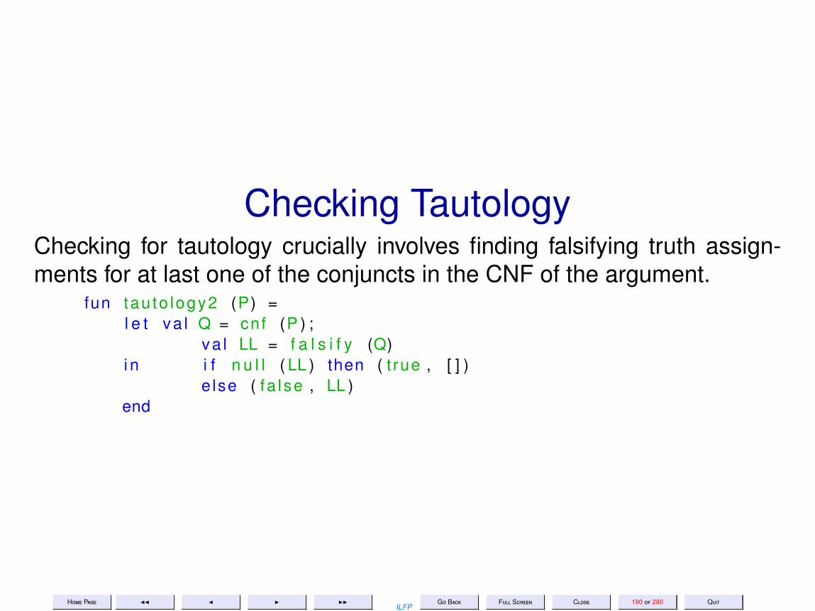
Home Page JJ J I IIILFP
Go Back Full Screen Close 190 of 280 Quit
Checking TautologyChecking for tautology crucially involves finding falsifying truth assign-ments for at last one of the conjuncts in the CNF of the argument.
fun tau to logy2 (P) =l e t va l Q = cnf (P ) ;
va l LL = f a l s i f y (Q)i n i f n u l l ( LL ) then ( t rue , [ ] )
e lse ( fa l se , LL )end

Home Page JJ J I IIILFP
Go Back Full Screen Close 191 of 280 Quit
Computing the CNF1. Rewrite implications and equivalences2. Convert to NNF by pushing negation inward3. Distribute OR over AND

Home Page JJ J I IIILFP
Go Back Full Screen Close 192 of 280 Quit
cnflistlist.sml( ∗======================== THE SIGNATURE PropLogic ======================s ignature PropLogic =
s i gexcept ion Atom exceptiondatatype Prop =
ATOM of s t r i n g |
NOT of Prop |
AND of Prop ∗ Prop |
OR of Prop ∗ Prop |
IMP of Prop ∗ Prop |
EQL of Prop ∗ Proptype Argument = Prop l i s t ∗ Propval show : Prop −> uni tval showArg : Argument −> uni tval f a l s i f y A r g : Argument −> Prop l i s t l i s tval Valid : Argument −> bool ∗ Prop l i s t l i s t
end ;
( ∗ P r o p o s i t i o n a l formulas ∗ )
======================== THE STRUCTURE PL ====================== ∗ )( ∗ s t r u c t u r e PL : PropLogic = ∗ )s t r u c t u r e PL = ( ∗ This i s f o r debugging purposes only ∗ )s t r u c t
datatype Prop =ATOM of s t r i n g |
NOT of Prop |
AND of Prop ∗ Prop |
OR of Prop ∗ Prop |
IMP of Prop ∗ Prop |
EQL of Prop ∗ Prop;
( ∗ −−−−−−−−−−−−−−− Propos i t ions to CNFs −−−−−−−−−−−−−−−−−−−−− ∗ )
except ion Atom exception ;fun newatom ( s ) = i f s = "" then r a i s e Atom exception
e l s e (ATOM s ) ;

Home Page JJ J I IIILFP
Go Back Full Screen Close 193 of 280 Quit
fun drawChar ( c , n ) =i f n>0 then ( p r i n t ( s t r ( c ) ) ; drawChar ( c , ( n−1 ) ) )e l s e ( ) ;
fun show ( P ) =l e t fun drawTabs ( n ) = drawChar (# "\t" , n ) ;
fun showTreeTabs (ATOM a , n ) = ( drawTabs ( n ) ;p r i n t ( a ) ;p r i n t ( "\n" ))
| showTreeTabs (NOT ( P ) , n ) = ( drawTabs ( n ) ; p r i n t ( "NOT" ) ;showTreeTabs ( P , n+1))
| showTreeTabs (AND ( P , Q) , n ) =( showTreeTabs ( P , n +1 ) ;drawTabs ( n ) ; p r i n t ( "AND\n" ) ;showTreeTabs (Q, n+1))
| showTreeTabs (OR ( P , Q) , n ) =( showTreeTabs ( P , n +1 ) ;drawTabs ( n ) ; p r i n t ( "OR\n" ) ;showTreeTabs (Q, n+1))
| showTreeTabs ( IMP ( P , Q) , n ) =( showTreeTabs ( P , n +1 ) ;drawTabs ( n ) ; p r i n t ( "IMPLIES\n" ) ;showTreeTabs (Q, n+1))
| showTreeTabs (EQL ( P , Q) , n ) =( showTreeTabs ( P , n +1 ) ;drawTabs ( n ) ; p r i n t ( "IFF\n" ) ;showTreeTabs (Q, n+1))
;in ( p r i n t ( "\n" ) ; showTreeTabs ( P , 0 ) ; p r i n t ( "\n" ) )
end;
( ∗ The funct ion below evaluates a formula given a t r u t h assignment .

Home Page JJ J I IIILFP
Go Back Full Screen Close 194 of 280 Quit
The t r u t h assignment i s given as a l i s t of atoms t h a t are t rue( a l l other atoms are f a l s e ) .
∗ )
fun lookup ( x : Prop , [ ] ) = f a l s e| lookup ( x , h : : L ) = ( x = h ) o r e l s e lookup ( x , L );
fun eval (ATOM a , L ) = lookup (ATOM a , L )| eval (NOT ( P ) , L ) = i f eval ( P , L ) then f a l s e e l s e t rue| eval (AND ( P , Q) , L ) = eval ( P , L ) andalso eval (Q, L )| eval (OR ( P , Q) , L ) = eval ( P , L ) o r e l s e eval (Q, L )| eval ( IMP ( P , Q) , L ) = eval (OR (NOT ( P ) , Q) , L )| eval (EQL ( P , Q) , L ) = ( eval ( P , L ) = eval (Q, L ) );
( ∗ We could a l s o wri te a tautology checker with out using t r u t hassignments by f i r s t convert ing everything i n t o a normal form .
∗ )
( ∗ F i r s t rew r i te i m p l i c a t i o n s and equivalences ∗ )
fun rewr i te (ATOM a ) = ATOM a| rewr i te (NOT ( P ) ) = NOT ( rewr i te ( P ) )| rewr i te (AND ( P , Q) ) = AND ( rewr i te ( P ) , rewr i te (Q) )| rewr i te (OR ( P , Q) ) = OR ( rewr i t e ( P ) , rewr i t e (Q) )| rewr i te ( IMP ( P , Q) ) = OR (NOT ( rewr i t e ( P ) ) , r ewr i te (Q) )| rewr i te (EQL ( P , Q) ) = rewr i te (AND (IMP( P , Q) , IMP (Q, P ) ) );
( ∗ Convert a l l formulas not conta in ing IMP or EQL i n t o Negation NormalForm .
∗ )
fun nnf (ATOM a ) = ATOM a| nnf (NOT (ATOM a ) ) = NOT (ATOM a )| nnf (NOT (NOT ( P ) ) ) = nnf ( P )| nnf (AND ( P , Q) ) = AND ( nnf ( P ) , nnf (Q) )| nnf (NOT (AND ( P , Q) ) ) = nnf (OR (NOT ( P ) , NOT (Q) ) )| nnf (OR ( P , Q) ) = OR ( nnf ( P ) , nnf (Q) )

Home Page JJ J I IIILFP
Go Back Full Screen Close 195 of 280 Quit
| nnf (NOT (OR ( P , Q) ) ) = nnf (AND (NOT ( P ) , NOT (Q) ) );
( ∗ D i s t r i b u t e OR over AND to get a NNF i n t o CNF ∗ )
fun distOR ( P , AND (Q, R ) ) = AND ( distOR ( P , Q) , distOR ( P , R ) )| distOR (AND (Q, R) , P ) = AND ( distOR (Q, P ) , distOR (R , P ) )| distOR ( P , Q) = OR ( P , Q)
( ∗ Now the CNF can be e a s i l y computed ∗ )
fun c o n j o f d i s j (AND ( P , Q) ) = AND ( c o n j o f d i s j ( P ) , c o n j o f d i s j (Q) )| c o n j o f d i s j (OR ( P , Q) ) = distOR ( c o n j o f d i s j ( P ) , c o n j o f d i s j (Q) )| c o n j o f d i s j ( P ) = P;
fun cnf ( P ) = c o n j o f d i s j ( nnf ( rewr i t e ( P ) ) ) ;
( ∗ −−−−−−−−−−−−−−− Propos i t ions to CNFs ends −−−−−−−−−−−−−−−−−−−−− ∗ )
( ∗ −−−−−−−−−−−−−−− CNFs to l i s t s of l i s t s of l i t e r a l s −−−−−−−−−−−− ∗ )
( ∗ Convert a c lause i n t o a l i s t of l i t e r a l s ∗ )fun f lat tenOR (OR (A, B ) ) = ( f la t tenOR A) @ ( f lat tenOR B )| f la t tenOR C = [C] ( ∗ assuming C i s a l i t e r a l ∗ )
( ∗ Convert a CNF i n t o a l i s t of l i s t s of c l a u s e s ∗ )fun flattenAND (AND (Q, R ) ) = ( flattenAND Q) @ ( flattenAND R)| flattenAND ( P ) = [ f la t tenOR P ] ( ∗ assuming P i s a c lause ∗ )
( ∗ Sor t the l i t L i s t L i s t using some ordering and remove d u p l i c a t e s while s o r t i n g ∗ )
( ∗ Define an ordering l i t L e s s on l i t e r a l s : ∗ )
fun l i t L e s s (ATOM ( a ) , ATOM ( b ) ) = a < b ( ∗ l e x i c o g r a p h i c ∗ )| l i t L e s s (NOT(ATOM a ) , NOT(ATOM b ) ) = a < b
( ∗ every negat ive l i t e r a l i s smal ler than every p o s i t i v e l i t e r a l ∗ )| l i t L e s s (NOT(ATOM a ) , ATOM ( b ) ) = t rue| l i t L e s s (ATOM ( a ) , NOT(ATOM b ) ) = f a l s e
( ∗ Extend the ordering to l i s t s of l i t e r a l s ∗ )

Home Page JJ J I IIILFP
Go Back Full Screen Close 196 of 280 Quit
fun c lauseLess ( [ ] , [ ] ) = f a l s e| c lauseLess ( [ ] , ) = t rue| c lauseLess ( , [ ] ) = f a l s e| c lauseLess ( h1 : : T1 , h2 : : T2 ) =
( l i t L e s s ( h1 , h2 ) ) o r e l s e( ( h1=h2 ) andalso c lauseLess ( T1 , T2 ) )
( ∗ Define mergeSortRD to remove d u p l i c a t e s as s o r t i n g proceeds ∗ )
fun mergeSortRD R [ ] = [ ]| mergeSortRD R [ h ] = [ h ]| mergeSortRD R L = ( ∗ can ’ t s p l i t a l i s t unless i t has > 1 element ∗ )l e t fun s p l i t [ ] = ( [ ] , [ ] )
| s p l i t [ h ] = ( [ h ] , [ ] )| s p l i t ( h1 : : h2 : : t ) =
l e t val ( l e f t , r i g h t ) = s p l i t t ;in ( h1 : : l e f t , h2 : : r i g h t )
end ;val ( l e f t , r i g h t ) = s p l i t L ;fun mergeRD (R , [ ] , [ ] ) = [ ]| mergeRD (R , [ ] , L2 ) = L2| mergeRD (R , L1 , [ ] ) = L1| mergeRD (R , ( L1 as h1 : : t 1 ) , ( L2 as h2 : : t 2 ) ) =
i f h1=h2 then mergeRD (R , t1 , L2 ) ( ∗ remove a copy ∗ )e l s e i f R( h1 , h2 ) then h1 : : ( mergeRD (R , t1 , L2 ) )e l s e h2 : : ( mergeRD (R , L1 , t2 ) ) ;
val s o r t e d L e f t = mergeSortRD R l e f t ;val sor tedRight = mergeSortRD R r i g h t ;
in mergeRD (R , sor tedLef t , sor tedRight )end ;
( ∗ Now s o r t the l i s t of l i s t s of l i t e r a l s removing d u p l i c a t e s ∗ )
fun sortRD LL = ( ∗ F i r s t s o r t each c lause and then the l i s t of c l a u s e s ∗ )l e t val sortedClauses = map ( mergeSortRD l i t L e s s ) LLin mergeSortRD clauseLess sortedClausesend ;
( ∗ Putt ing everything together ∗ )

Home Page JJ J I IIILFP
Go Back Full Screen Close 197 of 280 Quit
fun p r o p 2 l i s t l i s t P = sortRD ( flattenAND ( cnf P ) )end ( ∗ s t r u c t ∗ ) ;
open PL ;
( ∗ Test ing p r o p 2 l i s t l i s t ====================================− val god = ATOM ”There i s a God” ;val god = ATOM ”There i s a God” : Prop− val o s c i e n t = ATOM ”God i s omniscient ” ;val opotent = ATOM ”God i s omnipotent ” ;val e v i l = ATOM ”There i s E v i l ” ;val know = ATOM ”God knows there i s E v i l ” ;val prevent = ATOM ”God prevents E v i l ” ;
val hy1 = IMP ( god , AND ( osc ient , opotent ) ) ;val hy2 = IMP ( osc ient , know ) ;val hy3 = IMP ( opotent , prevent ) ;val hy4 = e v i l ;val conc = NOT ( god ) ;
val o s c i e n t = ATOM ”God i s omniscient ” : Prop− GC # 0 . 0 . 0 . 1 . 7 . 1 8 7 : (1 ms)val opotent = ATOM ”God i s omnipotent ” : Prop− val e v i l = ATOM ”There i s E v i l ” : Prop− val know = ATOM ”God knows there i s E v i l ” : Prop− val prevent = ATOM ”God prevents E v i l ” : Prop− − val hy1 = IMP (ATOM ”There i s a God” ,AND (ATOM # ,ATOM # ) ) : Prop− val hy2 = IMP (ATOM ”God i s omniscient ” ,ATOM ”God knows there i s E v i l ” ) : Prop− val hy3 = IMP (ATOM ”God i s omnipotent ” ,ATOM ”God prevents E v i l ” ) : Prop− val hy4 = ATOM ”There i s E v i l ” : Prop− val conc = NOT (ATOM ”There i s a God”) : Prop− − p r o p 2 l i s t l i s t hy1 ;val i t =
[ [NOT (ATOM ”There i s a God” ) ,ATOM ”God i s omnipotent ” ] ,[NOT (ATOM ”There i s a God” ) ,ATOM ”God i s omniscient ” ] ] : Prop l i s t l i s t
− p r o p 2 l i s t l i s t hy2 ;val i t = [ [NOT (ATOM ”God i s omniscient ” ) ,ATOM ”God knows there i s E v i l ” ] ]
: Prop l i s t l i s t− val andhyp = AND ( hy1 , AND ( hy2 , AND( hy3 , hy4 ) ) ) ;val andhyp = AND (IMP (ATOM # ,AND # ) ,AND (IMP # ,AND # ) ) : Prop− p r o p 2 l i s t l i s t andhyp ;
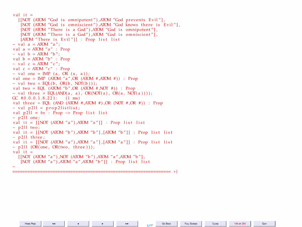
Home Page JJ J I IIILFP
Go Back Full Screen Close 198 of 280 Quit
val i t =[ [NOT (ATOM ”God i s omnipotent ” ) ,ATOM ”God prevents E v i l ” ] ,
[NOT (ATOM ”God i s omniscient ” ) ,ATOM ”God knows there i s E v i l ” ] ,[NOT (ATOM ”There i s a God” ) ,ATOM ”God i s omnipotent ” ] ,[NOT (ATOM ”There i s a God” ) ,ATOM ”God i s omniscient ” ] ,[ATOM ” There i s E v i l ” ] ] : Prop l i s t l i s t
− val a = ATOM ”a ” ;val a = ATOM ”a” : Prop− val b = ATOM ”b ” ;val b = ATOM ”b” : Prop− val c = ATOM ” c ” ;val c = ATOM ” c ” : Prop− val one = IMP ( a , OR ( a , a ) ) ;val one = IMP (ATOM ”a ” ,OR (ATOM # ,ATOM # ) ) : Prop− val two = EQL( b , OR( b , NOT( b ) ) ) ;val two = EQL (ATOM ”b ” ,OR (ATOM # ,NOT # ) ) : Prop− val three = EQL(AND( a , a ) , OR(NOT( a ) , OR( a , NOT( a ) ) ) ) ;GC # 0 . 0 . 0 . 1 . 8 . 2 2 1 : (1 ms)val three = EQL (AND (ATOM # ,ATOM # ) ,OR (NOT # ,OR # ) ) : Prop− val p 2 l l = p r o p 2 l i s t l i s t ;val p 2 l l = fn : Prop −> Prop l i s t l i s t− p 2 l l one ;val i t = [ [NOT (ATOM ”a ” ) ,ATOM ”a ” ] ] : Prop l i s t l i s t− p 2 l l two ;val i t = [ [NOT (ATOM ”b ” ) ,ATOM ”b ” ] , [ATOM ”b ” ] ] : Prop l i s t l i s t− p 2 l l three ;val i t = [ [NOT (ATOM ”a ” ) ,ATOM ”a ” ] , [ATOM ”a ” ] ] : Prop l i s t l i s t− p 2 l l (OR( one , OR( two , three ) ) ) ;val i t =
[ [NOT (ATOM ”a ” ) ,NOT (ATOM ”b ” ) ,ATOM ”a ” ,ATOM ”b ” ] ,[NOT (ATOM ”a ” ) ,ATOM ”a ” ,ATOM ”b ” ] ] : Prop l i s t l i s t
−
=============================================================== ∗ )

Home Page JJ J I IIILFP
Go Back Full Screen Close 199 of 280 Quit
Falsifying CNF1. Suffices to find a falsification of at least one conjunct2. A conjunct in the CNF can be false iff all the disjuncts in it are false.3. A disjunct is false iff it does not contain a “complementary pair”.
Assume the CNF is Q ≡∧m
i=1 Di where each Di ≡∨ni
j=1 Li j where theliterals of Di = Pi ∪ Ni where Pi is the set of positive literals (atoms) andNi consists of the atoms appearing as negative literals.
Then Di is false iff Pi ∩Ni = ∅.

Home Page JJ J I IIILFP
Go Back Full Screen Close 200 of 280 Quit
tautology1.sml
s ignature PropLogic =
s i gexcept ion Atom exceptiondatatype Prop =
ATOM of s t r i n g |
NOT of Prop |
AND of Prop ∗ Prop |
OR of Prop ∗ Prop |
IMP of Prop ∗ Prop |
EQL of Prop ∗ Proptype Argument = Prop l i s t ∗ Propval show : Prop −> uni tval showArg : Argument −> uni tval f a l s i f y A r g : Argument −> Prop l i s t l i s tval Valid : Argument −> bool ∗ Prop l i s t l i s t
end ;
( ∗ P r o p o s i t i o n a l formulas ∗ )
s t r u c t u r e PL : PropLogic =( ∗ s t r u c t u r e PL = ∗ ) ( ∗ This i s f o r debugging purposes only ∗ )s t r u c t
datatype Prop =ATOM of s t r i n g |
NOT of Prop |
AND of Prop ∗ Prop |
OR of Prop ∗ Prop |
IMP of Prop ∗ Prop |
EQL of Prop ∗ Prop;
except ion Atom exception ;fun newatom ( s ) = i f s = "" then r a i s e Atom exception
e l s e (ATOM s ) ;fun drawChar ( c , n ) =
i f n>0 then ( p r i n t ( s t r ( c ) ) ; drawChar ( c , ( n−1 ) ) )e l s e ( ) ;
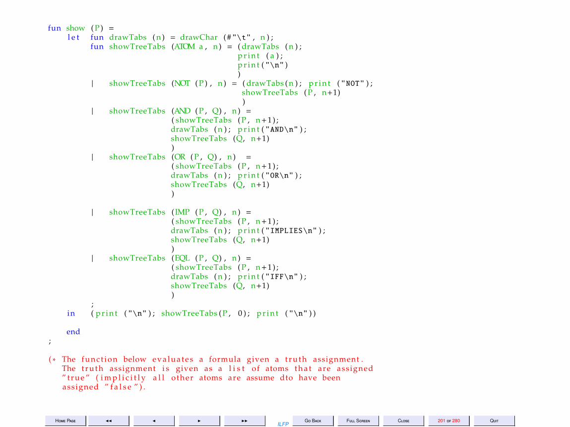
Home Page JJ J I IIILFP
Go Back Full Screen Close 201 of 280 Quit
fun show ( P ) =l e t fun drawTabs ( n ) = drawChar (# "\t" , n ) ;
fun showTreeTabs (ATOM a , n ) = ( drawTabs ( n ) ;p r i n t ( a ) ;p r i n t ( "\n" ))
| showTreeTabs (NOT ( P ) , n ) = ( drawTabs ( n ) ; p r i n t ( "NOT" ) ;showTreeTabs ( P , n+1))
| showTreeTabs (AND ( P , Q) , n ) =( showTreeTabs ( P , n +1 ) ;drawTabs ( n ) ; p r i n t ( "AND\n" ) ;showTreeTabs (Q, n+1))
| showTreeTabs (OR ( P , Q) , n ) =( showTreeTabs ( P , n +1 ) ;drawTabs ( n ) ; p r i n t ( "OR\n" ) ;showTreeTabs (Q, n+1))
| showTreeTabs ( IMP ( P , Q) , n ) =( showTreeTabs ( P , n +1 ) ;drawTabs ( n ) ; p r i n t ( "IMPLIES\n" ) ;showTreeTabs (Q, n+1))
| showTreeTabs (EQL ( P , Q) , n ) =( showTreeTabs ( P , n +1 ) ;drawTabs ( n ) ; p r i n t ( "IFF\n" ) ;showTreeTabs (Q, n+1))
;in ( p r i n t ( "\n" ) ; showTreeTabs ( P , 0 ) ; p r i n t ( "\n" ) )
end;
( ∗ The funct ion below evaluates a formula given a t r u t h assignment .The t r u t h assignment i s given as a l i s t of atoms t h a t are assigned” true ” ( i m p l i c i t l y a l l other atoms are assume dto have beenassigned ” f a l s e ” ) .

Home Page JJ J I IIILFP
Go Back Full Screen Close 202 of 280 Quit
∗ )
fun lookup ( x : Prop , [ ] ) = f a l s e| lookup ( x , h : : L ) =
i f ( x = h ) then truee l s e lookup ( x , L )
;
fun eval (ATOM a , L ) = lookup (ATOM a , L )| eval (NOT ( P ) , L ) = i f eval ( P , L ) then f a l s e e l s e t rue| eval (AND ( P , Q) , L ) = eval ( P , L ) andalso eval (Q, L )| eval (OR ( P , Q) , L ) = eval ( P , L ) o r e l s e eval (Q, L )| eval ( IMP ( P , Q) , L ) = eval (OR (NOT ( P ) , Q) , L )| eval (EQL ( P , Q) , L ) = ( eval ( P , L ) = eval (Q, L ) );
( ∗ We f i r s t convert every propos i t ion i n t o a normal form .∗ )
( ∗ F i r s t rew r i te i m p l i c a t i o n s and equivalences ∗ )
fun rewr i te (ATOM a ) = ATOM a| rewr i te (NOT ( P ) ) = NOT ( rewr i te ( P ) )| rewr i te (AND ( P , Q) ) = AND ( rewr i te ( P ) , rewr i te (Q) )| rewr i te (OR ( P , Q) ) = OR ( rewr i t e ( P ) , rewr i te (Q) )| rewr i te ( IMP ( P , Q) ) = OR (NOT ( rewr i te ( P ) ) , r ewr i te (Q) )| rewr i te (EQL ( P , Q) ) = rewr i te (AND (IMP( P , Q) , IMP (Q, P ) ) );
( ∗ Convert a l l formulas not conta in ing IMP or EQL i n t o Negation NormalForm .
∗ )
fun nnf (ATOM a ) = ATOM a| nnf (NOT (ATOM a ) ) = NOT (ATOM a )| nnf (NOT (NOT ( P ) ) ) = nnf ( P )| nnf (AND ( P , Q) ) = AND ( nnf ( P ) , nnf (Q) )| nnf (NOT (AND ( P , Q) ) ) = nnf (OR (NOT ( P ) , NOT (Q) ) )| nnf (OR ( P , Q) ) = OR ( nnf ( P ) , nnf (Q) )| nnf (NOT (OR ( P , Q) ) ) = nnf (AND (NOT ( P ) , NOT (Q) ) )

Home Page JJ J I IIILFP
Go Back Full Screen Close 203 of 280 Quit
;
( ∗ D i s t r i b u t e OR over AND to get a NNF i n t o CNF ∗ )
fun distOR ( P , AND (Q, R ) ) = AND ( distOR ( P , Q) , distOR ( P , R ) )| distOR (AND (Q, R) , P ) = AND ( distOR (Q, P ) , distOR (R , P ) )| distOR ( P , Q) = OR ( P , Q)
( ∗ Now the CNF can be e a s i l y computed ∗ )
fun c o n j o f d i s j (AND ( P , Q) ) = AND ( c o n j o f d i s j ( P ) , c o n j o f d i s j (Q) )| c o n j o f d i s j (OR ( P , Q) ) = distOR ( c o n j o f d i s j ( P ) , c o n j o f d i s j (Q) )| c o n j o f d i s j ( P ) = P;
fun cnf ( P ) = c o n j o f d i s j ( nnf ( rewr i t e ( P ) ) ) ;
( ∗ A propos i t ion in CNF i s a tautologyi f f
Every conjunct i s a tautologyi f f
Every d i s j u n c t in every conjunct conta ins both p o s i t i v e and negat ivel i t e r a l s of a t l e a s t one atom
So we c o n s t r u c t the l i s t of a l l the p o s i t i v e and negat ive atoms in everyd i s j u n c t to check whether the l i s t s are a l l equal . We need a binaryfunct ion on l i s t s to determine whether two l i s t s are d i s j o i n t
∗ )
fun i s P r e s e n t ( a , [ ] ) = f a l s e| i s P r e s e n t ( a , b : : L ) = ( a = b ) o r e l s e i s P r e s e n t ( a , L );
fun d i s j o i n t ( [ ] , M) = t rue| d i s j o i n t ( L , [ ] ) = t rue| d i s j o i n t ( L as a : : LL , M as b : :MM)=
not ( i s P r e s e n t ( a , M) ) andalsonot ( i s P r e s e n t ( b , L ) ) andalsod i s j o i n t ( LL , MM)
;

Home Page JJ J I IIILFP
Go Back Full Screen Close 204 of 280 Quit
( ∗ ABHISHEK : Defining a t o t a l ordering on atoms ( l e x i c o g r a p h i cordering on underlying s t r i n g s ) , and extending i t to a l i s t of atoms .
∗ )
except ion notAtom ;
fun atomLess ( a , b ) = case ( a , b ) of(ATOM( x ) , ATOM( y ) ) => x<y
| ( , ) => r a i s e notAtom ;
fun l i s t L e s s ( a , b ) = case ( a , b ) of( , [ ] ) => f a l s e
| ( [ ] , ) => t rue| ( x : : lx , y : : ly ) => i f atomLess ( x , y ) then true
e l s e i f atomLess ( y , x ) then f a l s ee l s e l i s t L e s s ( lx , ly ) ;
( ∗ ABHISHEK : Once we have a l i s t of f a l s i f i e r s , we would want to removeany dupl icat ion , f i r s t l y of atoms within a f a l s i f i e r , and secondly off a l s i f i e r s themselves .
In order to do t h i s , we maintain a l l l i s t s in some sorted order .Ins tead of s o r t i n g a l i s t with a poss ib ly l a r g e number of dupl ica tes ,we check f o r d u p l i c a t e s while i n s e r t i n g , and omit i n s e r t i o n i f aprevious i n s t a n c e i s detec ted .
∗ )
fun merge l e s s ( [ ] , l 2 ) = l 2| merge l e s s ( l1 , [ ] ) = l 1| merge l e s s ( x : : l1 , y : : l 2 ) =
i f l e s s ( x , y ) then x : : merge l e s s ( l1 , y : : l 2 )e l s e i f l e s s ( y , x ) then y : : merge l e s s ( x : : l1 , l 2 )e l s e merge l e s s ( x : : l1 , l 2 ) ;
( ∗ ABHISHEK : Claim i s t h a t i f a l l l i s t s are b u i l t through the abovefunct ion , then there i s no need to s o r t or remove d u p l i c a t e s .
Hence a l l ’@’ operat ions have been replaced by merge .∗ )

Home Page JJ J I IIILFP
Go Back Full Screen Close 205 of 280 Quit
except ion not CNF ;
fun p o s i t i v e s (ATOM a ) = [ATOM a ]| p o s i t i v e s (NOT (ATOM ))= [ ]| p o s i t i v e s (OR ( P , Q) ) = merge atomLess ( p o s i t i v e s ( P ) , p o s i t i v e s (Q) )| p o s i t i v e s ( P ) = r a i s e not CNF;
fun negat ives (ATOM ) = [ ]| negat ives (NOT (ATOM a ))= [ATOM a ]| negat ives (OR ( P , Q) ) = merge atomLess ( negat ives ( P ) , negat ives (Q) )| negat ives ( P ) = r a i s e not CNF;
( ∗ Check whether a formula in CNF i s a tautology ∗ )
fun t a u t (AND ( P , Q) ) = t a u t ( P ) andalso t a u t (Q)| t a u t ( P ) = ( ∗ i f i t i s not a con junct ion then i t must be a d i s j u n c t ∗ )
not ( d i s j o i n t ( p o s i t i v e s ( P ) , negat ives ( P ) ) );
fun tautology1 ( P ) =l e t val Q = cnf ( P )in t a u t (Q)end
;
( ∗ The main problem with the above i s t h a t i t checks whether a givenpropos i t ion i s a tautology , but whenever i t i s not , i t does not y i e l da f a l s i f y i n g t r u t h assignment . We r e c t i f y t h i s problem below .
∗ )
( ∗F i r s t l y , as in the case of the funct ion lookup , we w i l l assume a t r u t hassignment i s a l i s t of atoms which are assigned the t r u t h value ” true ”and t h a t any atom t h a t i s not present in the l i s t has been assigned” f a l s e ” .
Assume Q i s a propos i t ion in CNF. Then i t i s only necessary to l i s t outa l l the l i s t s of t r u t h assignments t h a t can f a l s i f y Q.

Home Page JJ J I IIILFP
Go Back Full Screen Close 206 of 280 Quit
Suppose Q i s in CNF, but not n e c e s s a r i l y a tautology . Further l e t
Q = AND (D1 , . . . , Dn)
where each Di i s a d i s j u n c t i o n of l i t e r a l s . Each Di = Pi + Ni wherePi and Ni are the l i s t s of atoms denoting the p o s i t i v e and negat ivel i t e r a l s r e s p e c t i v e l y .
Q would be ” f a l s i f i e d ” i f a t l e a s t one of the Di can be made f a l s e . Dican be made f a l s e only i f i t does not conta in a ”complementary pa i r ” ,i . e . there e x i s t s no atom a such t h a t both a and ˜ a occur in Di . Hencef o r Di to be f a l s i f i e d i t i s necessary t h a t the l i s t s Pi and Ni ared i s j o i n t ( i f there i s no atom common to Pi and Ni , there i s no”complementary pa i r ” in Di .
S ince Di i s a d i s j u n c t i o n of l i t e r a l s , i t can be f a l s i f i e d only byass igning every l i t e r a l in Di the value ” f a l s e ” . This can be done onlyby ass igning a l l the atoms in Pi the value ” f a l s e ” and a l l the atomsin Ni the value ” true ” .
In other words , i f Pi and Ni are d i s j o i n t , then Ni i s a t r u t hassignment which f a l s i f i e s the propos i t ion Q. We r e f e r to Ni as aFALSIFIER of Q.
Therefore the FALSIFIERS of Q are e x a c t l y the l i s t of negat ive atomsof each d i s j u n c t which does not conta in a complementary pa i r . Bychecking each d i s j u n c t in Q we may l i s t out ALL the p o s s i b l eFALSIFIERS of Q.
I f Q has no FALSIFIER then no d i s j u n c t Di can be made f a l s e i . e . everyd i s j u n c t does indeed have a compementary pai r . We may then concludet h a t Q i s a tautology .
∗ )
( ∗ The fol lowing funct ion assumes Q i s in CNF and outputs a l i s t of l i s tof atoms t h a t can f a l s i f y Q. I f t h i s l i s t of l i s t of atoms i s empty thenc l e a r l y Q i s a tautology .
∗ )
fun f a l s i f y (Q) =

Home Page JJ J I IIILFP
Go Back Full Screen Close 207 of 280 Quit
l e t fun l i s t F a l s i f i e r s (AND (A, B ) ) =merge l i s t L e s s ( l i s t F a l s i f i e r s (A) , l i s t F a l s i f i e r s ( B ) )
| l i s t F a l s i f i e r s (A) = ( ∗ Assume A i s a d i s j u n c t of l i t e r a l s ∗ )l e t val PLA = p o s i t i v e s (A) ( ∗ no uniq required ∗ )
val NLA = negat ives (A)in i f d i s j o i n t (PLA, NLA) then [NLA]
e l s e [ ]end
in l i s t F a l s i f i e r s (Q)end
;
fun tautology2 ( P ) =l e t val Q = cnf ( P ) ;
val LL = f a l s i f y (Q)in i f n u l l ( LL ) then ( true , [ ] )
e l s e ( f a l s e , LL )end
;
val tautology = tautology2 ;
( ∗We may use the tautology checker to prove various argumentsl o g i c a l l y va l id or l o g i c a l l y i n v a l i d . An argument c o n s i s t sof a s e t of pr opos i t i ons c a l l e d the ” hypotheses ” and a ( s i n g l e )propos i t ion c a l l e d the ” conclus ion ” . Loosely speaking , an argumenti s s i m i l a r to a theorem of mathematics . The argumenti s l o g i c a l l y va l id i f the conclus ion i s a l o g i c a l consequence ofof the hypotheses . More accura te ly , i f in every t r u t h assignmentwhich makes a l l the hypotheses true , the conclus ion i s a l s o i n v a r i a b l ytrue then the argument i s l o g i c a l l y va l id .
Symbol ica l ly i f H1, . . . , Hm are prop os i t io ns and C i s anotherpropos i t ion then the argument ( H1, . . . , Hm , C) i s l o g i c a l l yva l id ( equiva lent ly , C i s a l o g i c a l consequence of H1, . . . , Hm )i f and only i f the ( compound ) propos i t ion
(H1 / \ . . . / \ Hm) => C
i s a tautology .

Home Page JJ J I IIILFP
Go Back Full Screen Close 208 of 280 Quit
An argument which i s not l o g i c a l l y va l id i s l o g i c a l l yi n v a l i d . In p a r t i c u l a r i f there e x i s t s a t r u t h assignment under whicha l l the hypotheses are t rue but the conclus ion i s f a l s e , then theargument i s i n v a l i d .
Any argument i s t r i v i a l l y l o g i c a l l y va l id i f there i s no t r u t hassignment under which every hypothesis i s t rue . In other words ,i f the s e t of hypotheses i s an i n c o n s i s t e n t s e t then r e g a r d l e s sof what the conclus ion is , the argument i s always l o g i c a l l y va l id .The s e t of hypotheses H1, . . . , Hm i s ” i n c o n s i s t e n t ” i f and only i f(H1 / \ . . . / \ Hm) i s a ” c o n t r a d i c t i o n ” ( i t i s f a l s e f o r every t r u t hassignment ) .
∗ )type Argument = Prop l i s t ∗ Prop ;
fun showArg (A: Argument ) =l e t fun printArg (A: Argument as ( [ ] , c ) ) =
( drawChar (# "-" , 8 0 ) ; p r i n t ( "\n" ) ;show ( c ) ; p r i n t ( "\n\n" )
)| printArg (A: Argument as ( p : : p l i s t , c ) ) =
( show ( p ) ; p r i n t ( "\n" ) ;printArg ( p l i s t , c )
)in ( p r i n t ( "\n\n" ) ; printArg (A) )end
;
fun le f tReduce ( F ) =l e t except ion empty l i s t ;
fun l r ( [ ] ) = r a i s e empty l i s t| l r ( [ a ] ) = a| l r ( a : : L ) = F ( a , l r ( L ) )
in l rend
;
val bigAND = l e f tReduce (AND) ;

Home Page JJ J I IIILFP
Go Back Full Screen Close 209 of 280 Quit
fun Valid ( ( L , P ) : Argument ) =i f n u l l ( L ) then tautology ( P )e l s e tautology (IMP (bigAND ( L ) , P ) )
;
fun f a l s i f y A r g ( ( L , P ) : Argument ) =i f n u l l ( L ) then f a l s i f y ( cnf ( P ) )e l s e f a l s i f y ( cnf ( IMP (bigAND ( L ) , P ) ) )
;
end ( ∗ s t r u c t ∗ ) ;
( ∗ open PL ; ∗ )
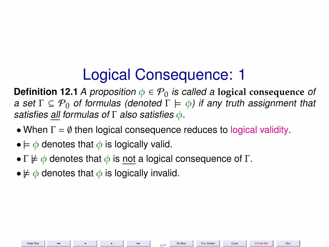
Home Page JJ J I IIILFP
Go Back Full Screen Close 210 of 280 Quit
Logical Consequence: 1Definition 12.1 A proposition φ ∈ P0 is called a logical consequence ofa set Γ ⊆ P0 of formulas (denoted Γ |= φ) if any truth assignment thatsatisfies all formulas of Γ also satisfies φ.
•When Γ = ∅ then logical consequence reduces to logical validity.• |= φ denotes that φ is logically valid.• Γ 6|= φ denotes that φ is not a logical consequence of Γ.• 6|= φ denotes that φ is logically invalid.

Home Page JJ J I IIILFP
Go Back Full Screen Close 211 of 280 Quit
Logical Consequence: 2Theorem 12.2 Let Γ = φi | 1 ≤ i ≤ n be a finite set of propositions, andlet ψ be any proposition. Then Γ |= ψ if and only if ((. . . ((φ1 ∧ φ2) ∧ φ3) ∧. . . ∧ φn)→ ψ) is a tautology.

Home Page JJ J I IIILFP
Go Back Full Screen Close 212 of 280 Quit
Other TheoremsTheorem 12.3 Let Γ = φi | 1 ≤ i ≤ n be a finite set of propositions, andlet ψ be any proposition. Then1. Γ |= ψ if and only if |= φ1→ (φ2→ · · · (φn→ ψ) · · · )
2. Γ |= ψ if and only if ((. . . ((φ1∧φ2)∧φ3)∧. . .∧φn)∧¬ψ) is a contradiction.
Corollary 12.4 A formula φ is a tautology iff ¬φ is a contradiction (unsat-isfiable).

Home Page JJ J I IIILFP
Go Back Full Screen Close 215 of 280 Quit
13. Lecture 13: Example: Tautology Checking (Contd)
Lecture 13: Example: Tautology Checking(Contd)
Wednesday 24 Aug 2011

Home Page JJ J I IIILFP
Go Back Full Screen Close 216 of 280 Quit
tautology1.sml – the full source
s ignature PropLogic =
s i gexcept ion Atom exceptiondatatype Prop =
ATOM of s t r i n g |
NOT of Prop |
AND of Prop ∗ Prop |
OR of Prop ∗ Prop |
IMP of Prop ∗ Prop |
EQL of Prop ∗ Proptype Argument = Prop l i s t ∗ Propval show : Prop −> uni tval showArg : Argument −> uni tval f a l s i f y A r g : Argument −> Prop l i s t l i s tval Valid : Argument −> bool ∗ Prop l i s t l i s t
end ;
( ∗ P r o p o s i t i o n a l formulas ∗ )
s t r u c t u r e PL : PropLogic =( ∗ s t r u c t u r e PL = ∗ ) ( ∗ This i s f o r debugging purposes only ∗ )s t r u c t
datatype Prop =ATOM of s t r i n g |
NOT of Prop |
AND of Prop ∗ Prop |
OR of Prop ∗ Prop |
IMP of Prop ∗ Prop |
EQL of Prop ∗ Prop;
except ion Atom exception ;fun newatom ( s ) = i f s = "" then r a i s e Atom exception
e l s e (ATOM s ) ;fun drawChar ( c , n ) =
i f n>0 then ( p r i n t ( s t r ( c ) ) ; drawChar ( c , ( n−1 ) ) )e l s e ( ) ;

Home Page JJ J I IIILFP
Go Back Full Screen Close 217 of 280 Quit
fun show ( P ) =l e t fun drawTabs ( n ) = drawChar (# "\t" , n ) ;
fun showTreeTabs (ATOM a , n ) = ( drawTabs ( n ) ;p r i n t ( a ) ;p r i n t ( "\n" ))
| showTreeTabs (NOT ( P ) , n ) = ( drawTabs ( n ) ; p r i n t ( "NOT" ) ;showTreeTabs ( P , n+1))
| showTreeTabs (AND ( P , Q) , n ) =( showTreeTabs ( P , n +1 ) ;drawTabs ( n ) ; p r i n t ( "AND\n" ) ;showTreeTabs (Q, n+1))
| showTreeTabs (OR ( P , Q) , n ) =( showTreeTabs ( P , n +1 ) ;drawTabs ( n ) ; p r i n t ( "OR\n" ) ;showTreeTabs (Q, n+1))
| showTreeTabs ( IMP ( P , Q) , n ) =( showTreeTabs ( P , n +1 ) ;drawTabs ( n ) ; p r i n t ( "IMPLIES\n" ) ;showTreeTabs (Q, n+1))
| showTreeTabs (EQL ( P , Q) , n ) =( showTreeTabs ( P , n +1 ) ;drawTabs ( n ) ; p r i n t ( "IFF\n" ) ;showTreeTabs (Q, n+1))
;in ( p r i n t ( "\n" ) ; showTreeTabs ( P , 0 ) ; p r i n t ( "\n" ) )
end;
( ∗ The funct ion below evaluates a formula given a t r u t h assignment .The t r u t h assignment i s given as a l i s t of atoms t h a t are assigned” true ” ( i m p l i c i t l y a l l other atoms are assume dto have beenassigned ” f a l s e ” ) .
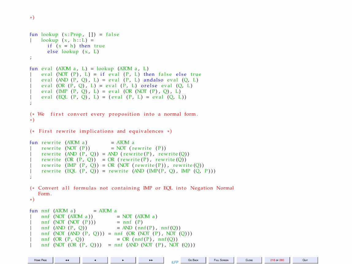
Home Page JJ J I IIILFP
Go Back Full Screen Close 218 of 280 Quit
∗ )
fun lookup ( x : Prop , [ ] ) = f a l s e| lookup ( x , h : : L ) =
i f ( x = h ) then truee l s e lookup ( x , L )
;
fun eval (ATOM a , L ) = lookup (ATOM a , L )| eval (NOT ( P ) , L ) = i f eval ( P , L ) then f a l s e e l s e t rue| eval (AND ( P , Q) , L ) = eval ( P , L ) andalso eval (Q, L )| eval (OR ( P , Q) , L ) = eval ( P , L ) o r e l s e eval (Q, L )| eval ( IMP ( P , Q) , L ) = eval (OR (NOT ( P ) , Q) , L )| eval (EQL ( P , Q) , L ) = ( eval ( P , L ) = eval (Q, L ) );
( ∗ We f i r s t convert every propos i t ion i n t o a normal form .∗ )
( ∗ F i r s t rew r i te i m p l i c a t i o n s and equivalences ∗ )
fun rewr i te (ATOM a ) = ATOM a| rewr i te (NOT ( P ) ) = NOT ( rewr i te ( P ) )| rewr i te (AND ( P , Q) ) = AND ( rewr i te ( P ) , rewr i te (Q) )| rewr i te (OR ( P , Q) ) = OR ( rewr i t e ( P ) , rewr i te (Q) )| rewr i te ( IMP ( P , Q) ) = OR (NOT ( rewr i te ( P ) ) , r ewr i te (Q) )| rewr i te (EQL ( P , Q) ) = rewr i te (AND (IMP( P , Q) , IMP (Q, P ) ) );
( ∗ Convert a l l formulas not conta in ing IMP or EQL i n t o Negation NormalForm .
∗ )
fun nnf (ATOM a ) = ATOM a| nnf (NOT (ATOM a ) ) = NOT (ATOM a )| nnf (NOT (NOT ( P ) ) ) = nnf ( P )| nnf (AND ( P , Q) ) = AND ( nnf ( P ) , nnf (Q) )| nnf (NOT (AND ( P , Q) ) ) = nnf (OR (NOT ( P ) , NOT (Q) ) )| nnf (OR ( P , Q) ) = OR ( nnf ( P ) , nnf (Q) )| nnf (NOT (OR ( P , Q) ) ) = nnf (AND (NOT ( P ) , NOT (Q) ) )

Home Page JJ J I IIILFP
Go Back Full Screen Close 219 of 280 Quit
;
( ∗ D i s t r i b u t e OR over AND to get a NNF i n t o CNF ∗ )
fun distOR ( P , AND (Q, R ) ) = AND ( distOR ( P , Q) , distOR ( P , R ) )| distOR (AND (Q, R) , P ) = AND ( distOR (Q, P ) , distOR (R , P ) )| distOR ( P , Q) = OR ( P , Q)
( ∗ Now the CNF can be e a s i l y computed ∗ )
fun c o n j o f d i s j (AND ( P , Q) ) = AND ( c o n j o f d i s j ( P ) , c o n j o f d i s j (Q) )| c o n j o f d i s j (OR ( P , Q) ) = distOR ( c o n j o f d i s j ( P ) , c o n j o f d i s j (Q) )| c o n j o f d i s j ( P ) = P;
fun cnf ( P ) = c o n j o f d i s j ( nnf ( rewr i t e ( P ) ) ) ;
( ∗ A propos i t ion in CNF i s a tautologyi f f
Every conjunct i s a tautologyi f f
Every d i s j u n c t in every conjunct conta ins both p o s i t i v e and negat ivel i t e r a l s of a t l e a s t one atom
So we c o n s t r u c t the l i s t of a l l the p o s i t i v e and negat ive atoms in everyd i s j u n c t to check whether the l i s t s are a l l equal . We need a binaryfunct ion on l i s t s to determine whether two l i s t s are d i s j o i n t
∗ )
fun i s P r e s e n t ( a , [ ] ) = f a l s e| i s P r e s e n t ( a , b : : L ) = ( a = b ) o r e l s e i s P r e s e n t ( a , L );
fun d i s j o i n t ( [ ] , M) = t rue| d i s j o i n t ( L , [ ] ) = t rue| d i s j o i n t ( L as a : : LL , M as b : :MM)=
not ( i s P r e s e n t ( a , M) ) andalsonot ( i s P r e s e n t ( b , L ) ) andalsod i s j o i n t ( LL , MM)
;

Home Page JJ J I IIILFP
Go Back Full Screen Close 220 of 280 Quit
( ∗ ABHISHEK : Defining a t o t a l ordering on atoms ( l e x i c o g r a p h i cordering on underlying s t r i n g s ) , and extending i t to a l i s t of atoms .
∗ )
except ion notAtom ;
fun atomLess ( a , b ) = case ( a , b ) of(ATOM( x ) , ATOM( y ) ) => x<y
| ( , ) => r a i s e notAtom ;
fun l i s t L e s s ( a , b ) = case ( a , b ) of( , [ ] ) => f a l s e
| ( [ ] , ) => t rue| ( x : : lx , y : : ly ) => i f atomLess ( x , y ) then true
e l s e i f atomLess ( y , x ) then f a l s ee l s e l i s t L e s s ( lx , ly ) ;
( ∗ ABHISHEK : Once we have a l i s t of f a l s i f i e r s , we would want to removeany dupl icat ion , f i r s t l y of atoms within a f a l s i f i e r , and secondly off a l s i f i e r s themselves .
In order to do t h i s , we maintain a l l l i s t s in some sorted order .Ins tead of s o r t i n g a l i s t with a poss ib ly l a r g e number of dupl ica tes ,we check f o r d u p l i c a t e s while i n s e r t i n g , and omit i n s e r t i o n i f aprevious i n s t a n c e i s detec ted .
∗ )
fun merge l e s s ( [ ] , l 2 ) = l 2| merge l e s s ( l1 , [ ] ) = l 1| merge l e s s ( x : : l1 , y : : l 2 ) =
i f l e s s ( x , y ) then x : : merge l e s s ( l1 , y : : l 2 )e l s e i f l e s s ( y , x ) then y : : merge l e s s ( x : : l1 , l 2 )e l s e merge l e s s ( x : : l1 , l 2 ) ;
( ∗ ABHISHEK : Claim i s t h a t i f a l l l i s t s are b u i l t through the abovefunct ion , then there i s no need to s o r t or remove d u p l i c a t e s .
Hence a l l ’@’ operat ions have been replaced by merge .∗ )

Home Page JJ J I IIILFP
Go Back Full Screen Close 221 of 280 Quit
except ion not CNF ;
fun p o s i t i v e s (ATOM a ) = [ATOM a ]| p o s i t i v e s (NOT (ATOM ))= [ ]| p o s i t i v e s (OR ( P , Q) ) = merge atomLess ( p o s i t i v e s ( P ) , p o s i t i v e s (Q) )| p o s i t i v e s ( P ) = r a i s e not CNF;
fun negat ives (ATOM ) = [ ]| negat ives (NOT (ATOM a ))= [ATOM a ]| negat ives (OR ( P , Q) ) = merge atomLess ( negat ives ( P ) , negat ives (Q) )| negat ives ( P ) = r a i s e not CNF;
( ∗ Check whether a formula in CNF i s a tautology ∗ )
fun t a u t (AND ( P , Q) ) = t a u t ( P ) andalso t a u t (Q)| t a u t ( P ) = ( ∗ i f i t i s not a con junct ion then i t must be a d i s j u n c t ∗ )
not ( d i s j o i n t ( p o s i t i v e s ( P ) , negat ives ( P ) ) );
fun tautology1 ( P ) =l e t val Q = cnf ( P )in t a u t (Q)end
;
( ∗ The main problem with the above i s t h a t i t checks whether a givenpropos i t ion i s a tautology , but whenever i t i s not , i t does not y i e l da f a l s i f y i n g t r u t h assignment . We r e c t i f y t h i s problem below .
∗ )
( ∗F i r s t l y , as in the case of the funct ion lookup , we w i l l assume a t r u t hassignment i s a l i s t of atoms which are assigned the t r u t h value ” true ”and t h a t any atom t h a t i s not present in the l i s t has been assigned” f a l s e ” .
Assume Q i s a propos i t ion in CNF. Then i t i s only necessary to l i s t outa l l the l i s t s of t r u t h assignments t h a t can f a l s i f y Q.

Home Page JJ J I IIILFP
Go Back Full Screen Close 222 of 280 Quit
Suppose Q i s in CNF, but not n e c e s s a r i l y a tautology . Further l e t
Q = AND (D1 , . . . , Dn)
where each Di i s a d i s j u n c t i o n of l i t e r a l s . Each Di = Pi + Ni wherePi and Ni are the l i s t s of atoms denoting the p o s i t i v e and negat ivel i t e r a l s r e s p e c t i v e l y .
Q would be ” f a l s i f i e d ” i f a t l e a s t one of the Di can be made f a l s e . Dican be made f a l s e only i f i t does not conta in a ”complementary pa i r ” ,i . e . there e x i s t s no atom a such t h a t both a and ˜ a occur in Di . Hencef o r Di to be f a l s i f i e d i t i s necessary t h a t the l i s t s Pi and Ni ared i s j o i n t ( i f there i s no atom common to Pi and Ni , there i s no”complementary pa i r ” in Di .
S ince Di i s a d i s j u n c t i o n of l i t e r a l s , i t can be f a l s i f i e d only byass igning every l i t e r a l in Di the value ” f a l s e ” . This can be done onlyby ass igning a l l the atoms in Pi the value ” f a l s e ” and a l l the atomsin Ni the value ” true ” .
In other words , i f Pi and Ni are d i s j o i n t , then Ni i s a t r u t hassignment which f a l s i f i e s the propos i t ion Q. We r e f e r to Ni as aFALSIFIER of Q.
Therefore the FALSIFIERS of Q are e x a c t l y the l i s t of negat ive atomsof each d i s j u n c t which does not conta in a complementary pa i r . Bychecking each d i s j u n c t in Q we may l i s t out ALL the p o s s i b l eFALSIFIERS of Q.
I f Q has no FALSIFIER then no d i s j u n c t Di can be made f a l s e i . e . everyd i s j u n c t does indeed have a compementary pai r . We may then concludet h a t Q i s a tautology .
∗ )
( ∗ The fol lowing funct ion assumes Q i s in CNF and outputs a l i s t of l i s tof atoms t h a t can f a l s i f y Q. I f t h i s l i s t of l i s t of atoms i s empty thenc l e a r l y Q i s a tautology .
∗ )
fun f a l s i f y (Q) =
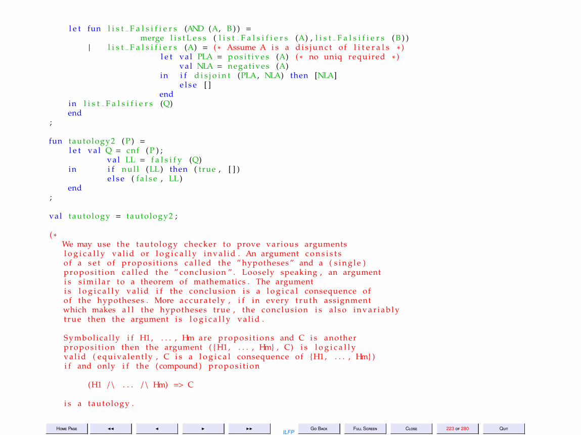
Home Page JJ J I IIILFP
Go Back Full Screen Close 223 of 280 Quit
l e t fun l i s t F a l s i f i e r s (AND (A, B ) ) =merge l i s t L e s s ( l i s t F a l s i f i e r s (A) , l i s t F a l s i f i e r s ( B ) )
| l i s t F a l s i f i e r s (A) = ( ∗ Assume A i s a d i s j u n c t of l i t e r a l s ∗ )l e t val PLA = p o s i t i v e s (A) ( ∗ no uniq required ∗ )
val NLA = negat ives (A)in i f d i s j o i n t (PLA, NLA) then [NLA]
e l s e [ ]end
in l i s t F a l s i f i e r s (Q)end
;
fun tautology2 ( P ) =l e t val Q = cnf ( P ) ;
val LL = f a l s i f y (Q)in i f n u l l ( LL ) then ( true , [ ] )
e l s e ( f a l s e , LL )end
;
val tautology = tautology2 ;
( ∗We may use the tautology checker to prove various argumentsl o g i c a l l y va l id or l o g i c a l l y i n v a l i d . An argument c o n s i s t sof a s e t of pr opos i t i ons c a l l e d the ” hypotheses ” and a ( s i n g l e )propos i t ion c a l l e d the ” conclus ion ” . Loosely speaking , an argumenti s s i m i l a r to a theorem of mathematics . The argumenti s l o g i c a l l y va l id i f the conclus ion i s a l o g i c a l consequence ofof the hypotheses . More accura te ly , i f in every t r u t h assignmentwhich makes a l l the hypotheses true , the conclus ion i s a l s o i n v a r i a b l ytrue then the argument i s l o g i c a l l y va l id .
Symbol ica l ly i f H1, . . . , Hm are prop os i t io ns and C i s anotherpropos i t ion then the argument ( H1, . . . , Hm , C) i s l o g i c a l l yva l id ( equiva lent ly , C i s a l o g i c a l consequence of H1, . . . , Hm )i f and only i f the ( compound ) propos i t ion
(H1 / \ . . . / \ Hm) => C
i s a tautology .

Home Page JJ J I IIILFP
Go Back Full Screen Close 224 of 280 Quit
An argument which i s not l o g i c a l l y va l id i s l o g i c a l l yi n v a l i d . In p a r t i c u l a r i f there e x i s t s a t r u t h assignment under whicha l l the hypotheses are t rue but the conclus ion i s f a l s e , then theargument i s i n v a l i d .
Any argument i s t r i v i a l l y l o g i c a l l y va l id i f there i s no t r u t hassignment under which every hypothesis i s t rue . In other words ,i f the s e t of hypotheses i s an i n c o n s i s t e n t s e t then r e g a r d l e s sof what the conclus ion is , the argument i s always l o g i c a l l y va l id .The s e t of hypotheses H1, . . . , Hm i s ” i n c o n s i s t e n t ” i f and only i f(H1 / \ . . . / \ Hm) i s a ” c o n t r a d i c t i o n ” ( i t i s f a l s e f o r every t r u t hassignment ) .
∗ )type Argument = Prop l i s t ∗ Prop ;
fun showArg (A: Argument ) =l e t fun printArg (A: Argument as ( [ ] , c ) ) =
( drawChar (# "-" , 8 0 ) ; p r i n t ( "\n" ) ;show ( c ) ; p r i n t ( "\n\n" )
)| printArg (A: Argument as ( p : : p l i s t , c ) ) =
( show ( p ) ; p r i n t ( "\n" ) ;printArg ( p l i s t , c )
)in ( p r i n t ( "\n\n" ) ; printArg (A) )end
;
fun le f tReduce ( F ) =l e t except ion empty l i s t ;
fun l r ( [ ] ) = r a i s e empty l i s t| l r ( [ a ] ) = a| l r ( a : : L ) = F ( a , l r ( L ) )
in l rend
;
val bigAND = l e f tReduce (AND) ;

Home Page JJ J I IIILFP
Go Back Full Screen Close 225 of 280 Quit
fun Valid ( ( L , P ) : Argument ) =i f n u l l ( L ) then tautology ( P )e l s e tautology (IMP (bigAND ( L ) , P ) )
;
fun f a l s i f y A r g ( ( L , P ) : Argument ) =i f n u l l ( L ) then f a l s i f y ( cnf ( P ) )e l s e f a l s i f y ( cnf ( IMP (bigAND ( L ) , P ) ) )
;
end ( ∗ s t r u c t ∗ ) ;
( ∗ open PL ; ∗ )

Home Page JJ J I IIILFP
Go Back Full Screen Close 227 of 280 Quit
14. Lecture 14: The Pure Untyped Lambda Calculus: Syntax
Lecture 14: The Pure Untyped LambdaCalculus: Syntax
Friday 26 Aug 2011

Home Page JJ J I IIILFP
Go Back Full Screen Close 230 of 280 Quit
15. Lecture 15: The Pure Untyped Lambda Calculus: Basics
Lecture 15: The Pure Untyped LambdaCalculus: Basics
Tuesday 30 Aug 2011

Home Page JJ J I IIILFP
Go Back Full Screen Close 231 of 280 Quit
Pure Untyped λ-Calculus: SyntaxThe language Λ of pure untyped λ-terms is the smallest set built up froman infinite set V of variables
L,M,N ::= x Variableλx[L] Abstraction(L M) Application
where x ∈ V.
• A Variable denotes a possible binding in the external environment.• An Abstraction denotes a function which takes a formal parameter.• An Application denotes the application of a function to an actual param-
eter.

Home Page JJ J I IIILFP
Go Back Full Screen Close 232 of 280 Quit
Free and Bound VariablesDefinition 15.1 For any term N the set of free variables and the set of allvariables are defined by induction on the structure of terms.
N FV(N) Var(N)x x xλx[L] FV(L) − x Var(L) ∪ x(L M) FV(L) ∪ FV(M) Var(L) ∪ Var(M)
• The set of bound variables BV(N) = Var(N) − FV(N).• The same variable name may be used with different bindings in a single
term (e.g. (λx[x] λx[(x y)]))• The brackets “[” and “]” delimit the scope of the bound variable x in the
term λx[L].•Λ0 ⊆ Λ is the set of λ-terms with no free variables.

Home Page JJ J I IIILFP
Go Back Full Screen Close 233 of 280 Quit
Notational ConventionsTo minimize use of brackets unambiguously1. λx1x2 . . . xm[L] denotes λx1[λx2[. . . λxm[L] · · · ]] i.e. L is the scope of
each of the variables x1, x2, . . . xm.2. (L1 L2 · · · Lm) denotes (· · · (L1 L2) · · · Lm) i.e. application is left-
associative.

Home Page JJ J I IIILFP
Go Back Full Screen Close 234 of 280 Quit
SubstitutionDefinition 15.2 For any terms L, M and N and any variable x, the substi-tution of the term N for a variable x is defined as follows:N/xx ≡ NN/xy ≡ y if y . xN/xλx[L] ≡ λx[L]N/xλy[L] ≡ λy[N/xL] if y . x and y < FV(N)N/xλy[L] ≡ λz[N/zz/xL] if y . x and y ∈ FV(N) and z is ’fresh’N/x(L M) ≡ (N/xL N/xM)
• In the above definition it is necessary to ensure that the free variablesof N continue to remain free after substitution.• The phrase “z is ’fresh”’ may be taken to mean z < FV(N) ∪ Var(L).• z could be fresh even if z ∈ BV(N)

Home Page JJ J I IIILFP
Go Back Full Screen Close 235 of 280 Quit
α-equivalenceDefinition 15.3 (α-equivalence) λx[L] ≡α λy[y/xL] provided y <Var(L).
•Here again if y ∈ FV(L) it must not be captured by a change of boundvariables.

Home Page JJ J I IIILFP
Go Back Full Screen Close 236 of 280 Quit
Untyped λ-Calculus: Basic β-ReductionDefinition 15.4• Any (sub-)term of the form (λx[L] M) is called a β-redex• Basic β-reduction is the relation
(λx[L] M)→β M/xL′ (6)
where L′ ≡α L.

Home Page JJ J I IIILFP
Go Back Full Screen Close 237 of 280 Quit
Untyped λ-Calculus: 1-step β-ReductionDefinition 15.5 A 1-step β-reduction→1
β is the smallest (under the ⊆ordering) relation such that
β1L→β ML→1
β M β1AbsL→1
β M
λx[L]→1β λx[M]
β1AppLL→1
β M
(L N)→1β (M N)
β1AppRL→1
β M
(N L)→1β (N M)
•→1β is the compatible closure of basic β-reduction to all contexts.
•We will often omit the superscript 1 as understood.

Home Page JJ J I IIILFP
Go Back Full Screen Close 238 of 280 Quit
Untyped λ-Calculus: β-ReductionDefinition 15.6• For all integers n ≥ 0, n-step β-reduction→n
β is defined by induction on1-step β-reduction
βnBasis L→0β
L βnInductionL→m
β M→1β N
L→m+1β N
(m ≥ 0)
• β-reduction→∗β is the reflexive-transitive closure of 1-step β-reduction.That is,
β∗L→n
β ML→∗β M (n ≥ 0)

Home Page JJ J I IIILFP
Go Back Full Screen Close 239 of 280 Quit
Untyped λ-Calculus: NormalizationDefinition 15.7• A term is called a β-normal form (β-nf) if it has no β-redexes.• A term is weakly normalising (β-WN) if it reduces to a β-normal form.• A term L is strong normalising (β-SN) if it has no infinite reduction se-
quence L→1β L1→
1β L2→
1β · · ·

Home Page JJ J I IIILFP
Go Back Full Screen Close 240 of 280 Quit
Untyped λ-Calculus: ExamplesExample 15.8
1. Kd f= λx y[x], I
d f= λx[x], S
d f= λx y z[((x z) (y z))], ω
d f= λx[(x x)] are all
β-nfs.
2. Ωd f= (ω ω) has no β-nf. Hence it is neither weakly nor strongly normal-
ising.3. (K (ω ω)) cannot reduce to any normal form because it has no finite
reduction sequences. All its reductions are of the form
(K (ω ω))→1β (K (ω ω))→1
β (K (ω ω))→1β · · ·
or at some point it could transform to
(K (ω ω))→1β λy[(ω ω)]→1
β λy[(ω ω)]→1β · · ·
4. ((K ω) Ω) is weakly normalising because it can reduce to the normalform ω but it is not strongly normalising because it also has an infinitereduction sequence
((K ω) Ω)→1β ((K ω) Ω)→1
β · · ·

Home Page JJ J I IIILFP
Go Back Full Screen Close 241 of 280 Quit
Examples of Strong NormalizationExample 15.91. ((K ω) ω) is strongly normalising because it reduces to the normal formω in a single step.
2. Consider the term ((S K) K). Its reduction sequences go as follows:
((S K) K)→1β λz[((K z) (K z))]→1
β λz[z] ≡ I

Home Page JJ J I IIILFP
Go Back Full Screen Close 244 of 280 Quit
16. Lecture 16: Notions of Reduction
Lecture 16: Notions of ReductionTuesday 06 Sep 2011

Home Page JJ J I IIILFP
Go Back Full Screen Close 245 of 280 Quit
ReductionFor any function such as p = λx[3.x.x + 4.x + 1],
(p 2) = 3.2.2 + 4.2 + 1 = 21
However there is something asymmetric about the identity, in the sensethat while (p 2) deterministically produces 3.2.2 + 4.2 + 1 which in turnsimplifies deterministically to 21, it is not possible to deterministically in-fer that 21 came from (p 2). It would be more accurate to refer to thissequence as a reduction sequence and capture the asymmetry as follows:
(p 2) ; 3.2.2 + 4.2 + 1 ; 21
And yet they are behaviourally equivalent and mutually substitutable in allcontexts (referentially transparent).
1. Reduction (specifically β-reduction) captures this asymmetry.2. Since reduction produces behaviourally equal terms we have the follow-
ing notion of equality.

Home Page JJ J I IIILFP
Go Back Full Screen Close 246 of 280 Quit
Untyped λ-Calculus: β-EqualityDefinition 16.1 β-equality or β-conversion (denoted =β) is the smallestequivalence relation containing β-reduction (→∗β).
The following are equivalent definitions.
1. =β is the reflexive-symmetric-transitive closure of 1-step β-reduction.2. =β is the smallest relation defined by the following rules.
=β BasisL→∗β ML =β M
=β Reflexivity L =β L
=β SymmetryL =β MM =β L =β Transitivity
L =β M, M =β NL =β N

Home Page JJ J I IIILFP
Go Back Full Screen Close 247 of 280 Quit
CompatibilityDefinition 16.2 A binary relation ρ ⊆ Λ × Λ is said to be compatible ifL ρ M implies1. for all variables x, λx[L] ρ λx[M] and2. for all terms N, (L N) ρ (M N) and (N L) ρ (N M).
Example 16.31. ≡α is a compatible relation2.→1
β is by definition a compatible relation.

Home Page JJ J I IIILFP
Go Back Full Screen Close 248 of 280 Quit
Compatibility of Beta-reduction andBeta-Equality
Theorem 16.4 β-reduction→∗β and β-equality =β are both compatible re-lations.
2
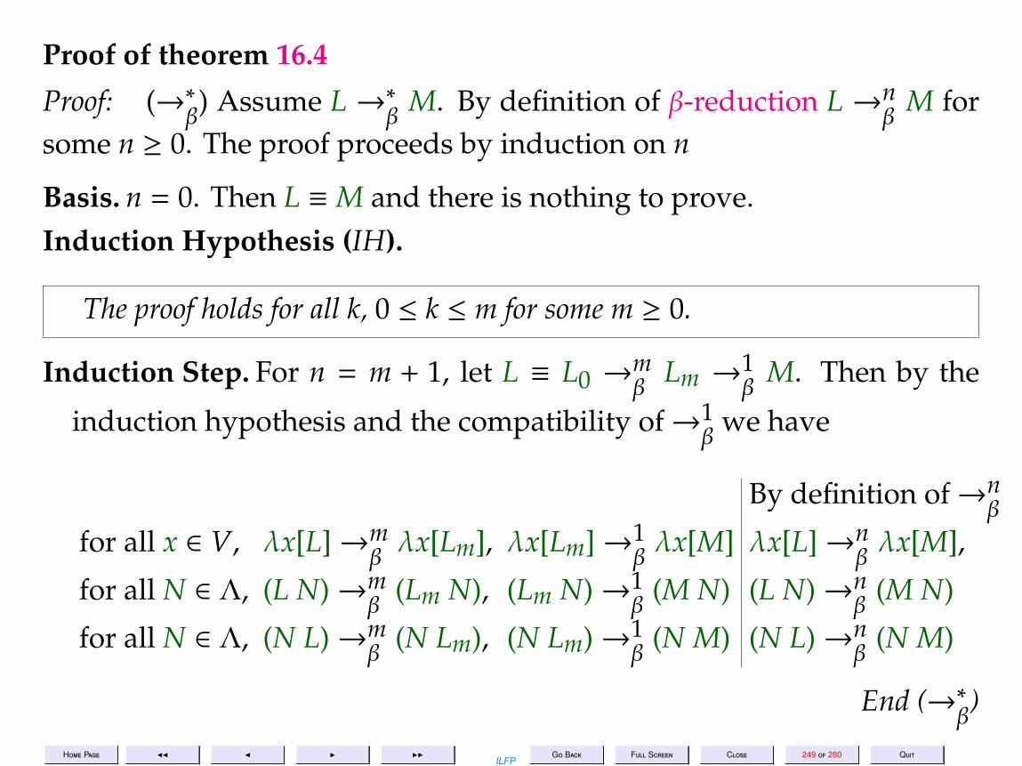
Home Page JJ J I IIILFP
Go Back Full Screen Close 249 of 280 Quit
Proof of theorem 16.4
Proof: (→∗β) Assume L →∗β M. By definition of β-reduction L →nβ M for
some n ≥ 0. The proof proceeds by induction on n
Basis. n = 0. Then L ≡M and there is nothing to prove.Induction Hypothesis (IH).
The proof holds for all k, 0 ≤ k ≤ m for some m ≥ 0.
Induction Step. For n = m + 1, let L ≡ L0 →mβ Lm →1
β M. Then by the
induction hypothesis and the compatibility of→1β we have
By definition of→nβ
for all x ∈ V, λx[L]→mβ λx[Lm], λx[Lm]→1
β λx[M] λx[L]→nβ λx[M],
for all N ∈ Λ, (L N)→mβ (Lm N), (Lm N)→1
β (M N) (L N)→nβ (M N)
for all N ∈ Λ, (N L)→mβ (N Lm), (N Lm)→1
β (N M) (N L)→nβ (N M)
End (→∗β)

Home Page JJ J I IIILFP
Go Back Full Screen Close 250 of 280 Quit
(=β) Assume L =β M. We proceed by induction on the length of the proofof L =β M using the definition of β-equality.
Basis. n = 1. Then either L ≡ M or L →∗β M. The case of reflexivity istrivial and the case of L→∗β M follows from the previous proof.
Induction Hypothesis (IH).
For all terms L and M, such that the proof of L =β M requires less than nsteps for n > 1, the compatibility result holds.
Induction Step. Suppose the proof requires n steps and the last step isobtained by use of either =β Symmetry or =β Transitivity on someprevious steps.Case (=β Symmetry). Then the (n − 1)-st step proved M =β L. By the
induction hypothesis and then by applying =β Symmetry to eachcase we get

Home Page JJ J I IIILFP
Go Back Full Screen Close 251 of 280 Quit
By =β Symmetryfor all variables x, λx[M] =β λx[L] λx[L] =β λx[M]for all terms N, (M N) =β (L N) (L N) =β (M N)for all terms N, (N M) =β (N L) (N M) =β (N L)
Case (=β Transitivity). Suppose L =β M was inferred in the n-th stepfrom two previous steps which proved L =β P and P =β M for someterm P. Then again by induction hypothesis and then applying =βTransitivity we get
By =β Transitivityfor all variables x, λx[L] =β λx[P], λx[P] =β λx[M] λx[L] =β λx[M]for all terms N, (L N) =β (P N), (P N) =β (M N) (L N) =β (M N)for all terms N, (N L) =β (N P), (N P) =β (N M) (N L) =β (N P)
End (=β)
QED

Home Page JJ J I IIILFP
Go Back Full Screen Close 252 of 280 Quit
Eta reductionGiven any term M and a variable x < FV(M), the syntax allows us toconstruct the term λx[(M x)] such that for every term N we have
(λx[(M x)] N)→1β (M N)
In other words,(λx[(M x)] N) =β (M N) for all terms N
We say that the two terms λx[(M x)] and M are extensionally equiva-lent i.e. they are syntactically distinct but there is no way to distinguishbetween their behaviours.So we define basic η-reduction as the relation
λx[(L x)]→η L provided x < FV(L) (7)

Home Page JJ J I IIILFP
Go Back Full Screen Close 253 of 280 Quit
Eta-Reduction and Eta-EqualityThe following notions are then defined similar to the corresponding no-tions for β-reduction.
• 1-step η-reduction→1η is the closure of basic η-reduction to all contexts,
•→nη is defined by induction on 1-step η-reduction
• η-reduction→∗η is the reflexive-transitive closure of 1-step η-reduction.
• the notions of strong and weak η normal forms η-nf.• the notion of η-equality or η-conversion denoted by =η.

Home Page JJ J I IIILFP
Go Back Full Screen Close 254 of 280 Quit
Exercise 16.1
1. Prove that η-reduction and η-equality are both compatible relations.2. Prove that η-reduction is strongly normalising.3. Define basic βη-reduction as the application of either (6) or (7). Now prove
that→1βη,→∗βη and =βη are all compatible relations.

Home Page JJ J I IIILFP
Go Back Full Screen Close 256 of 280 Quit
17. Lecture 17: Confluence Definitions
Lecture 17: Confluence DefinitionWednesday 07 Sep 2011

Home Page JJ J I IIILFP
Go Back Full Screen Close 257 of 280 Quit
Definition 17.1 For any binary relation ρ on a set A
1. ρ∗ is the least preorder containing ρ and is defined by the following rules.
Definition 17.2 Let ρ be any relation on terms. ρ has the diamond propertyif for all L, M, N,
Mρ
Lρ
N
⇒ ∃P :
Mρ
Pρ
N
Definition 17.3 Let −→ be a reduction relation, −→∗ the least preorder contain-ing −→ and ∗
←→ the least equivalence relation containing −→∗. Then
• −→ is terminating iff there is no infinite sequence of the form
L0 −→ L1 −→ · · ·
• −→ is locally confluent if for all L, M, N,
N←− L −→M⇒ ∃P : N −→∗ P ∗←−M
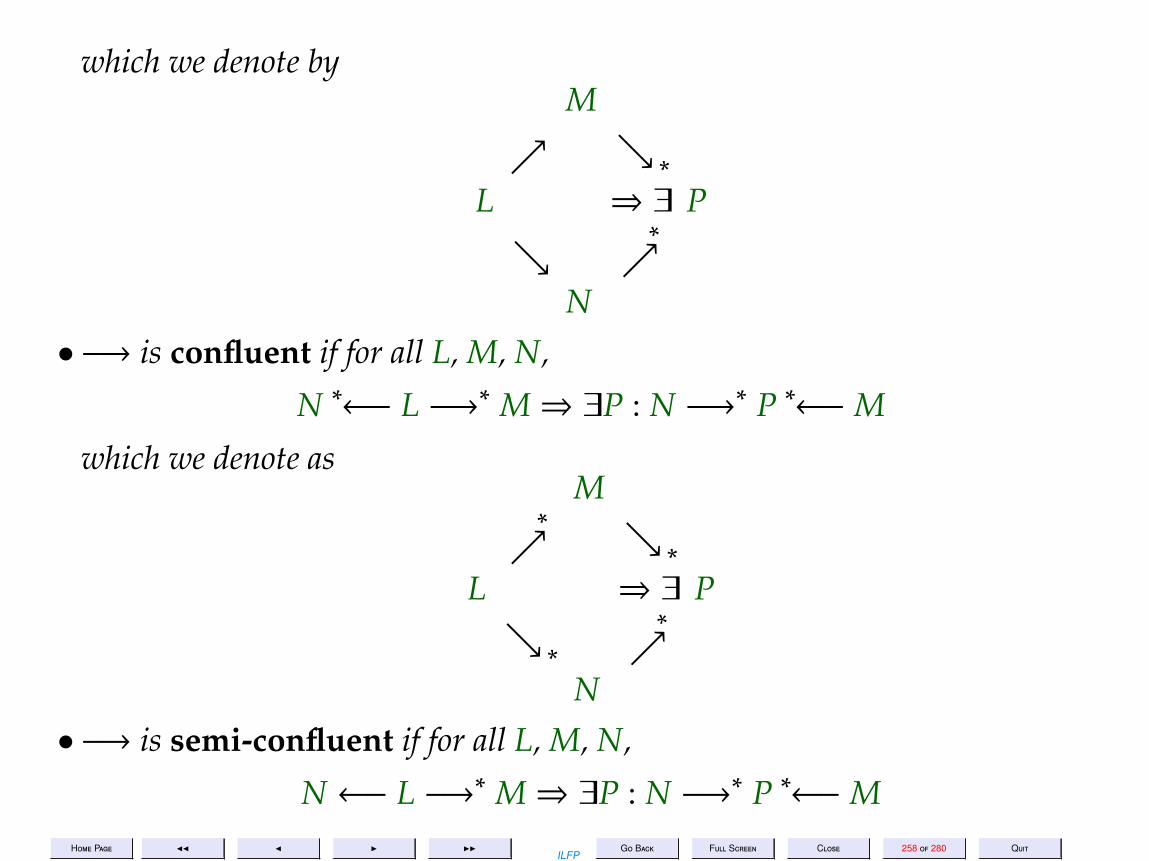
Home Page JJ J I IIILFP
Go Back Full Screen Close 258 of 280 Quit
which we denote byM
−→
−→∗
L ⇒ ∃ P−→
−→
∗
N• −→ is confluent if for all L, M, N,
N ∗←− L −→∗ M⇒ ∃P : N −→∗ P ∗←−M
which we denote asM
−→
∗ −→∗
L ⇒ ∃ P−→∗
−→
∗
N• −→ is semi-confluent if for all L, M, N,
N←− L −→∗ M⇒ ∃P : N −→∗ P ∗←−M

Home Page JJ J I IIILFP
Go Back Full Screen Close 259 of 280 Quit
which we denote byM
−→
−→∗
L ⇒ ∃ P−→∗
−→
∗
N• −→ is Church-Rosser if for all L, M,
L ∗←→M⇒ ∃P : L −→∗ P ∗←−M
which we denote byL ∗
←→ M−→∗ ⇓
−→
∗
∃P
Fact 17.4 Any confluent relation is also semi-confluent.
Lemma 17.5
1. ∗←→ is the least equivalence containing −→.

Home Page JJ J I IIILFP
Go Back Full Screen Close 260 of 280 Quit
2. ∗←→ is the least equivalence containing −→∗.
3. L ∗←→M if and only if there exists a finite sequence L ≡M0,M1, . . .Mm ≡M,
m ≥ 0 such that for each i, 0 ≤ i < m, Mi −→ Mi+1 or Mi+1 −→ Mi. Werepresent this fact more succinctly as
L ≡α M0 −→ /←−M1 −→ /←− · · · −→ /←−Mm ≡α M (8)
Proof:
1. Just prove that ∗←→ is a subset of every equivalence that contains −→.
2. Use induction on the length of proofs to prove this part3. For the last part it is easy to see that the existence of the “chain equation”
(8) implies L ∗←→M by transitivity. For the other part use induction on
the length of the proof.
QED

Home Page JJ J I IIILFP
Go Back Full Screen Close 262 of 280 Quit
18. Lecture 18: The Church-Rosser Property
Lecture 17: The Church-Rosser PropertyFriday 09 Sep 2011

Home Page JJ J I IIILFP
Go Back Full Screen Close 263 of 280 Quit
Definition 18.1 The parallel-β or ||β reduction is the smallest relation for which the followingrules hold.
||β1 L −→1||β L ||β1Abs1
L −→1||β L′
λx[L] −→1||β λx[L′]
||β1AppL −→1
||β L′,M −→1||β M′
(L M) −→1||β (L′ M′) ||β1Abs2
L −→1||β L′,M −→1
||β M′
(λx[L] M) −→1||β M
′/xL′
Lemma 18.2
1. L −→1β L′⇒ L −→1
||β L′.
2. L −→1||β L′⇒ L −→∗β L′.
3. The smallest preorder containing −→1||β is −→∗
||β=−→∗
β.
4. If L −→1β L′ and M −→1
||β M′ then M/xL −→1||β M
′/xL′.
Proof: By induction on the structure of terms or by induction on the number of steps inany proof. QED
Theorem 18.3 −→1||β has the diamond property.

Home Page JJ J I IIILFP
Go Back Full Screen Close 264 of 280 Quit
Proof: We need to prove for all L
N 1||β←− L −→1
||β M⇒ ∃P : N −→1||β P 1
||β←−M
We prove this by induction on the structure of L and a case analysis of the rule appliedin definition 18.1.
Case L ≡ x ∈ V. Then L ≡M ≡ N ≡ P.
Before dealing with the other inductive cases we dispose of some trivial sub-cases thatarise in some or all of them.
Case L ≡α M. Choose P ≡α N to complete the diamond.
Case L ≡α N. Then choose P ≡α M.
Case M ≡α N. Then there is nothing to prove.
In the sequel we assume N .α L .α M .α N and proceed by induction on the structureof L.
Case L ≡ λx[L1]. Then clearly M and N were both obtained in proofs whose last step wasan application of rule ||β1Abs1 and so M ≡ λx[M1] and N ≡ λx[N1] for some M1 and N1respectively and hence N1
1||β←− L1 −→
1||β M1. By the induction hypothesis we have
∃P1 : N1 −→1||β P1
1||β←−M1
Hence by choosing P ≡ λx[P1] we obtain the required result.
Case L ≡ (L1 L2) and L1 is not an abstraction.
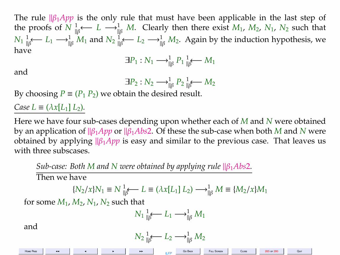
Home Page JJ J I IIILFP
Go Back Full Screen Close 265 of 280 Quit
The rule ||β1App is the only rule that must have been applicable in the last step ofthe proofs of N 1
||β←− L −→1||β M. Clearly then there exist M1, M2, N1, N2 such that
N11||β←− L1 −→
1||β M1 and N2
1||β←− L2 −→
1||β M2. Again by the induction hypothesis, we
have∃P1 : N1 −→
1||β P1
1||β←−M1
and∃P2 : N2 −→
1||β P2
1||β←−M2
By choosing P ≡ (P1 P2) we obtain the desired result.
Case L ≡ (λx[L1] L2).
Here we have four sub-cases depending upon whether each of M and N were obtainedby an application of ||β1App or ||β1Abs2. Of these the sub-case when both M and N wereobtained by applying ||β1App is easy and similar to the previous case. That leaves uswith three subscases.
Sub-case: Both M and N were obtained by applying rule ||β1Abs2.Then we have
N2/xN1 ≡ N 1||β←− L ≡ (λx[L1] L2) −→1
||β M ≡ M2/xM1
for some M1, M2, N1, N2 such thatN1
1||β←− L1 −→
1||β M1
andN2
1||β←− L2 −→
1||β M2

Home Page JJ J I IIILFP
Go Back Full Screen Close 266 of 280 Quit
By the induction hypothesis
∃P1 : N1 −→1||β P1
1||β←−M1
and∃P2 : N2 −→
1||β P2
1||β←−M2
and the last part of lemma 18.2 we have
∃P ≡ P2/xP1 : N −→1||β P 1
||β←−M
completing the proof.Sub-case: M was obtained by applying rule ||β1Abs2 and N by ||β1App.Then we have the form
(λx[N1] N2) ≡ N 1||β←− L ≡ (λx[L1] L2) −→1
||β M ≡ M2/xM1
where againN1
1||β←− L1 −→
1||β M1
andN2
1||β←− L2 −→
1||β M2
By the induction hypothesis
∃P1 : N1 −→1||β P1
1||β←−M1
and∃P2 : N2 −→
1||β P2
1||β←−M2

Home Page JJ J I IIILFP
Go Back Full Screen Close 267 of 280 Quit
and finally we have∃P ≡ P2/xP1 : N −→1
||β P 1||β←−M
completing the proof.Sub-case: M was obtained by applying rule ||β1App and N by ||β1Abs2.Similar to the previous sub-case.
QED
Theorem 18.4 −→1||β is confluent.
Proof: We need to show that for all L, M, N,
N ∗
||β←− L −→∗||β M⇒ ∃P : N −→∗
||β P ∗||β←−M
We prove this by induction on the length of the sequences
L −→1||β M1 −→
1||β M2 −→
1||β · · · −→
1||β Mm ≡M
andL −→1
||β N1 −→1||β N2 −→
1||β · · · −→
1||β Nn ≡ N
where m,n ≥ 0. More specifically we prove this by induction on the pairs of integers( j, i) bounded by (n,m), where ( j, i) < ( j′, i′) if and only if either j < j′ or ( j = j′) and i < i′.The interesting cases are those where both m,n > 0. So we repeatedly apply theorem

Home Page JJ J I IIILFP
Go Back Full Screen Close 268 of 280 Quit
18.3 to complete the rectangle
L −→1||β M1 −→
1||β M2 −→
1||β · · · −→
1||β Mm ≡M
||β↓1 ||β↓1 ||β↓1 · · · ||β↓1N1 −→
1||β P11 −→
1||β P12 −→
1||β · · · −→
1||β P1m
||β↓1 ||β↓1 ||β↓1 · · · ||β↓1... ... ... · · ·
...||β↓1 ||β↓1 ||β↓1 · · · ||β↓1Nn −→
1||β Pn1 −→
1||β Pn2 −→
1||β · · · −→
1||β Pnm ≡ P
QED
Corollary 18.5 −→1β is confluent.
Proof: Since −→∗β=−→∗
||β it follows from theorem 18.4 that −→1β is confluent. QED
Corollary 18.6 If a term reduces to a β-normal form then the normal form is unique (upto ≡α).
Proof: If N1∗
β←− L −→∗β N2 and both N1 N2 are β-nfs, then by the corollary 18.5 theymust both be β-reducible to a third element N3 which is impoosible if both N1 and N2are β-nfs. Hence β-nfs are unique whenever they exist. QED
Corollary 18.7 −→1β is Church-Rosser.
Proof: Follows from corollary 18.5 and theorem 19.1. QED

Home Page JJ J I IIILFP
Go Back Full Screen Close 270 of 280 Quit
19. Lecture 19: Confluence Characterizations
Lecture 19: Confluence CharacterizationTuesday 13 Sep 2011

Home Page JJ J I IIILFP
Go Back Full Screen Close 271 of 280 Quit
Theorem 19.1 The following statements are equivalent.
1. −→ is Church-Rosser.2. −→ is confluent.3. −→ is semi-confluent
Proof: (1⇒ 2) AssumeN ∗←− L −→∗ M
Clearly then N ∗←→M. If −→ is Church-Rosser then
∃P : N −→∗ P ∗←−M
which implies that it is confluent.
(2⇒ 3) Obviously any confluent relation is also semi-confluent.
(3⇒ 2) Assume L ∗←→ M. We proceed by induction on the length of the
chain (8).
L ≡α M0 −→ /←−M1 −→ /←− · · · −→ /←−Mm ≡α M
Basis. m = 0. This case is trivial since for any P, L −→∗ P iff M −→∗ P

Home Page JJ J I IIILFP
Go Back Full Screen Close 272 of 280 Quit
Induction Hypothesis (IH).
The claim is true for all chains of length k, 0 ≤ k < m.
Induction Step. Assume the chain is of length m = k + 1. i.e.
L ≡α M0 −→ /←−M1 −→ /←− · · · −→ /←−Mk −→ /←−Mk+1 ≡α M
Case Mk −→M. Then by the induction hypothesis and semi-confluencewe have
L ∗←→ Mk
−→∗ ⇓
−→
∗−→
∃Q M−→∗ ⇓
−→
∗
∃Pwhich proves the claim.Case Mk←−M. Then the claim follows from the induction hypothesis

Home Page JJ J I IIILFP
Go Back Full Screen Close 273 of 280 Quit
and the following diagram
L ∗←→ Mk←−M
−→∗ ⇓
−→
∗
∃P
QED
Lemma 19.2 If a terminating relation is locally confluent then it is semi-confluent.
Proof: Assume L −→ M and L −→∗ N. We need to show that thereexists P such that M −→
∗ P and N −→∗ P. We prove this by inductionon the length of L −→∗ N. If L ≡α N then P ≡α M, otherwise assumeL −→ N1 −→ · · · −→ Nn = N for some n > 0. By the local confluencewe have there exists P1 such that M −→∗ P1. By successively applyingthe induction hypothesis we get terms P2, . . . ,Pn such that P j−1 −→
∗ P jand N j −→
∗ P j for each j, 1 ≤ j ≤ m. In effect we complete the followingrectangle
L −→ N1 −→ N2 −→ · · · −→ Nn ≡M↓ ↓ ↓ · · · ↓
M −→ P1 −→ P2 −→ · · · −→ Pn

Home Page JJ J I IIILFP
Go Back Full Screen Close 274 of 280 Quit
QED
From lemma 19.2 and theorem 19.1 we have the following theorem.
Theorem 19.3 If a terminating relation is locally confluent then it is Church-Rosser and confluent.

Home Page JJ J I IIILFP
Go Back Full Screen Close 276 of 280 Quit
20. Lecture 25
Lecture 25: The Damas Milner AlgorithmTuesday 13 Sep 2011

Home Page JJ J I IIILFP
Go Back Full Screen Close 277 of 280 Quit
The Damas-Milner algorithm for Type Assignment
The algorithm W uses unification. Assume U(σ, τ) = V, where U is aunification algorithm on type expressions, which takes two monotypes σand τ as arguments and either fails or returns a substitution V which isthe mgu of σ and τ.
The INPUT: An expression e and a type environment A (which consistsof the assumptions about the types of some variables).
The OUTPUT: A substitution S and a type assignment τ to e.
The ALGORITHM: The algorithm W(A, e) = (S, τ), is presented by in-duction on the structure of e.
1. Case e ≡ x and A(x) = ∀α1 . . . αn[σ] . Then S = ε and for each newβi, 1 ≤ i ≤ n τ = σβi/αi | 1 ≤ i ≤ n.

Home Page JJ J I IIILFP
Go Back Full Screen Close 278 of 280 Quit
2. Case e ≡ (e1 e2). Then let W(A, e1) = (S1, τ1) and W(A, e2) = (S2, τ2) andU(τ1S2, τ2→ β) = V, where β is new. Then S = S1 S2 V and τ = βV.
3. Case e ≡ λx[e1]. Then let β be a new type variable, and A′ = x : β :: Abe a modified environment such that W(A′, e1) = (S1, τ1). Then S = S1and τ = βS1→ τ1.
4. Case e ≡ let x = e1 in e2. Let W(A, e1) = (S1, τ1), A′ = x : γ :: A, whereγ = τ1S1, A′′ = A′S1 and W(A′′, e2) = (S2, τ2). Then S = S2 S1 andτ = τ2.
5. When any of the above conditions is not met then W fails.

Home Page JJ J I IIILFP
Go Back Full Screen Close 279 of 280 Quit
References[1] F. Baader and T. Nipkow. Term Rewriting and All That. Cambridge Unviersity Press, Cambridge, U.K., 1998.
[2] H. P. Barendregt. The Lambda Calculus: Its Syntax and Semantics. Elsevier Science B. V., Amsterdam, TheNetherlands, 1984.
[3] R. Hindley and J. Seldin. Combinators, λ-calculus. London Mathematical Society, U.K., 1985.
[4] R. Sethi. Programming Languages (Second Edition). Addison-Wesley Publishing Company, New York, U.S.A.,1996.

Home Page JJ J I IIILFP
Go Back Full Screen Close 280 of 280 Quit
Thank You!Any Questions?