Embed Size (px)
Citation preview
Introduction to Location Discovery Lecture 7
September 28, 2006
EENG 460a / CPSC 436 / ENAS 960 Networked Embedded Systems &
Sensor Networks
Andreas [email protected]
Office: AKW 212Tel 432-1275
Course Websitehttp://www.eng.yale.edu/enalab/courses/2006f/eeng460a
Announcements
Next lecture class meets in CO-40 Make sure that you have access to the room You are responsible for trying out the
programming assignment and asking questions about it!!!
The lab session will show you how to use the nodes & tools in the lab
Why is Location Discovery(LD) Important?
Very fundamental component for many other services• GPS does not work everywhere• Smart Systems – devices need to know where they are• Geographic routing & coverage problems• People and asset tracking• Need spatial reference when monitoring spatial
phenomena We will use the node localization problem as a
platform for illustrating basic concepts from the course
Why spend so much time on LD?
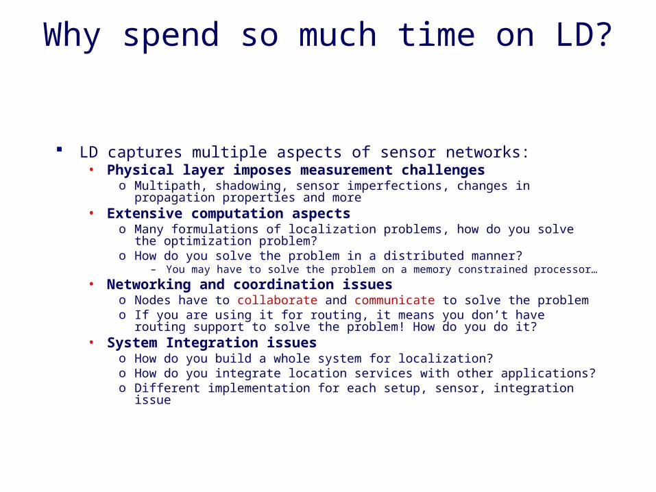
LD captures multiple aspects of sensor networks:• Physical layer imposes measurement challenges
o Multipath, shadowing, sensor imperfections, changes in propagation properties and more• Extensive computation aspects
o Many formulations of localization problems, how do you solve the optimization problem?
o How do you solve the problem in a distributed manner?– You may have to solve the problem on a memory constrained processor…
• Networking and coordination issueso Nodes have to collaborate and communicate to solve the problemo If you are using it for routing, it means you don’t have routing support to solve the
problem! How do you do it?• System Integration issues
o How do you build a whole system for localization?o How do you integrate location services with other applications?o Different implementation for each setup, sensor, integration issue
Taxonomy of Localization Mechanisms
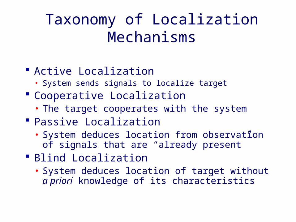
Active Localization• System sends signals to localize target
Cooperative Localization• The target cooperates with the system
Passive Localization• System deduces location from observation of signals
that are “already present” Blind Localization
• System deduces location of target without a priori knowledge of its characteristics

Active Mechanisms
Non-cooperative• System emits signal, deduces target location from
distortions in signal returns• e.g. radar and reflective sonar systems
Cooperative Target• Target emits a signal with known characteristics;
system deduces location by detecting signal• e.g. ORL Active Bat, GALORE Panel, AHLoS,
MIT Cricket Cooperative Infrastructure
• Elements of infrastructure emit signals; target deduces location from detection of signals
• e.g. GPS, MIT Cricket
TargetSynchronization channelRanging channel
Measurement Technologies
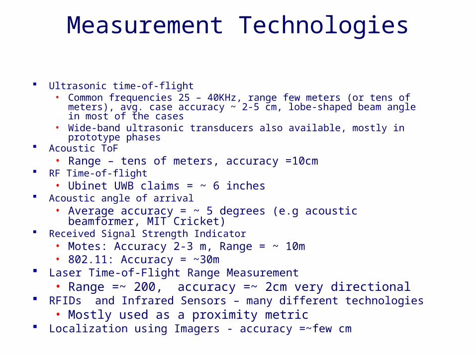
Ultrasonic time-of-flight• Common frequencies 25 – 40KHz, range few meters (or tens of meters), avg. case
accuracy ~ 2-5 cm, lobe-shaped beam angle in most of the cases• Wide-band ultrasonic transducers also available, mostly in prototype phases
Acoustic ToF
• Range – tens of meters, accuracy =10cm RF Time-of-flight
• Ubinet UWB claims = ~ 6 inches Acoustic angle of arrival
• Average accuracy = ~ 5 degrees (e.g acoustic beamformer, MIT Cricket) Received Signal Strength Indicator
• Motes: Accuracy 2-3 m, Range = ~ 10m• 802.11: Accuracy = ~30m
Laser Time-of-Flight Range Measurement• Range =~ 200, accuracy =~ 2cm very directional
RFIDs and Infrared Sensors – many different technologies• Mostly used as a proximity metric
Localization using Imagers - accuracy =~few cm
Some Existing Localization Systems
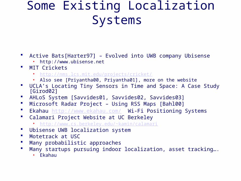
Active Bats[Harter97] – Evolved into UWB company Ubisense• http://www.ubisense.net
MIT Crickets• http://nms.lcs.mit.edu/projects/cricket/• Also see [Priyantha00, Priyantha01], more on the website
UCLA’s Locating Tiny Sensors in Time and Space: A Case Study [Girod02] AHLoS System [Savvides01, Savvides02, Savvides03] Microsoft Radar Project – Using RSS Maps [Bahl00] Ekahau http://www.ekahau.com/ Wi-Fi Positioning Systems Calamari Project Website at UC Berkeley
• http://www.cs.berkeley.edu/~kamin/calamari Ubisense UWB localization system Motetrack at USC Many probabilistic approaches Many startups pursuing indoor localization, asset tracking….
• Ekahau
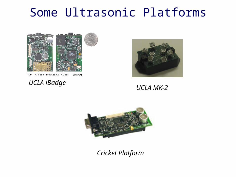
Some Ultrasonic Platforms
UCLA iBadgeUCLA MK-2
Cricket Platform
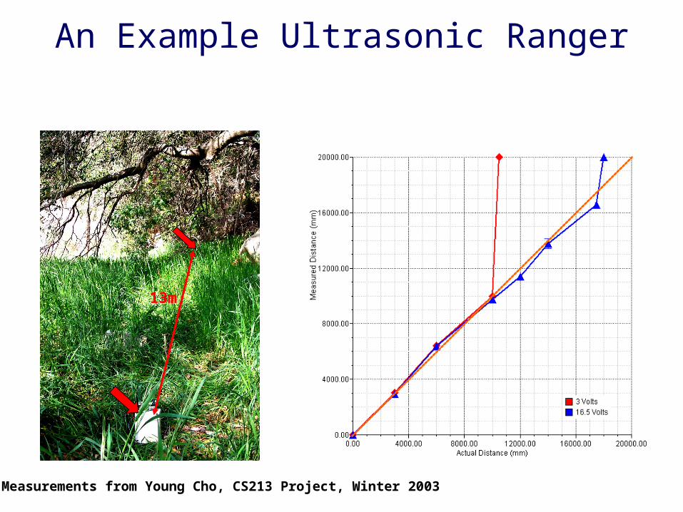
An Example Ultrasonic Ranger
13m
Measurements from Young Cho, CS213 Project, Winter 2003
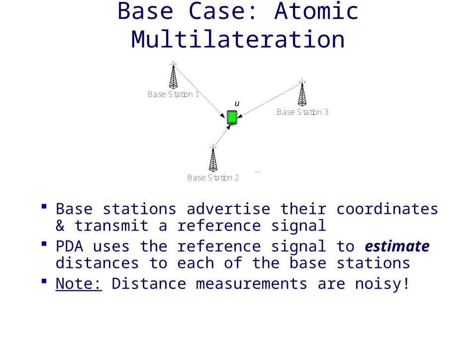
Base Case: Atomic Multilateration
Base stations advertise their coordinates & transmit a reference signal
PDA uses the reference signal to estimate distances to each of the base stations
Note: Distance measurements are noisy!
Base Station 1
Base Station 3
Base Station 2
u
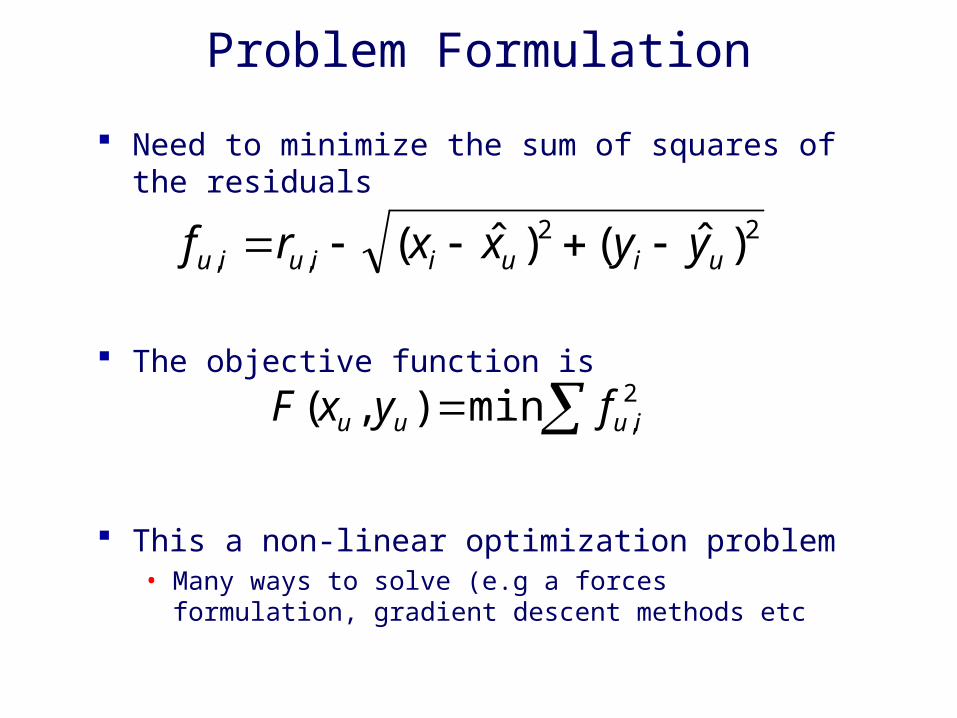
Problem Formulation
Need to minimize the sum of squares of the residuals
The objective function is
This a non-linear optimization problem• Many ways to solve (e.g a forces formulation, gradient
descent methods etc
22,, )ˆ()ˆ( uiuiiuiu yyxxrf
2,min),( iuuu fyxF
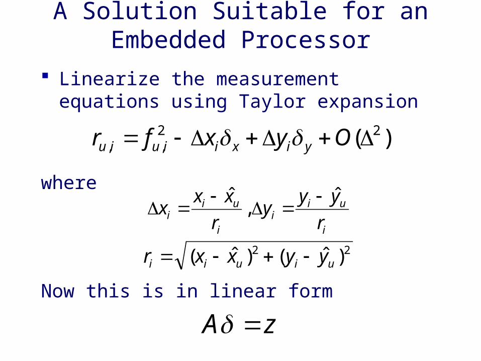
A Solution Suitable for an Embedded Processor
Linearize the measurement equations using Taylor expansion
where
Now this is in linear form
)( 22,, Oyxfr yixiiuiu
i
uii
i
uii r
yyy
r
xxx
ˆ,
ˆ
22 )ˆ()ˆ( uiuii yyxxr
zA
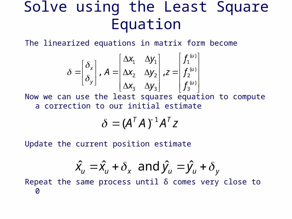
Solve using the Least Square Equation
The linearized equations in matrix form become
Now we can use the least squares equation to compute a correction to our initial estimate
Update the current position estimate
Repeat the same process until δ comes very close to 0
)(3
)(2
)(1
33
22
11
, ,u
u
u
y
x
f
f
f
z
yx
yx
yx
A
zAAA TT 1)(
yuuxuu yyxx ˆˆ and ˆˆ
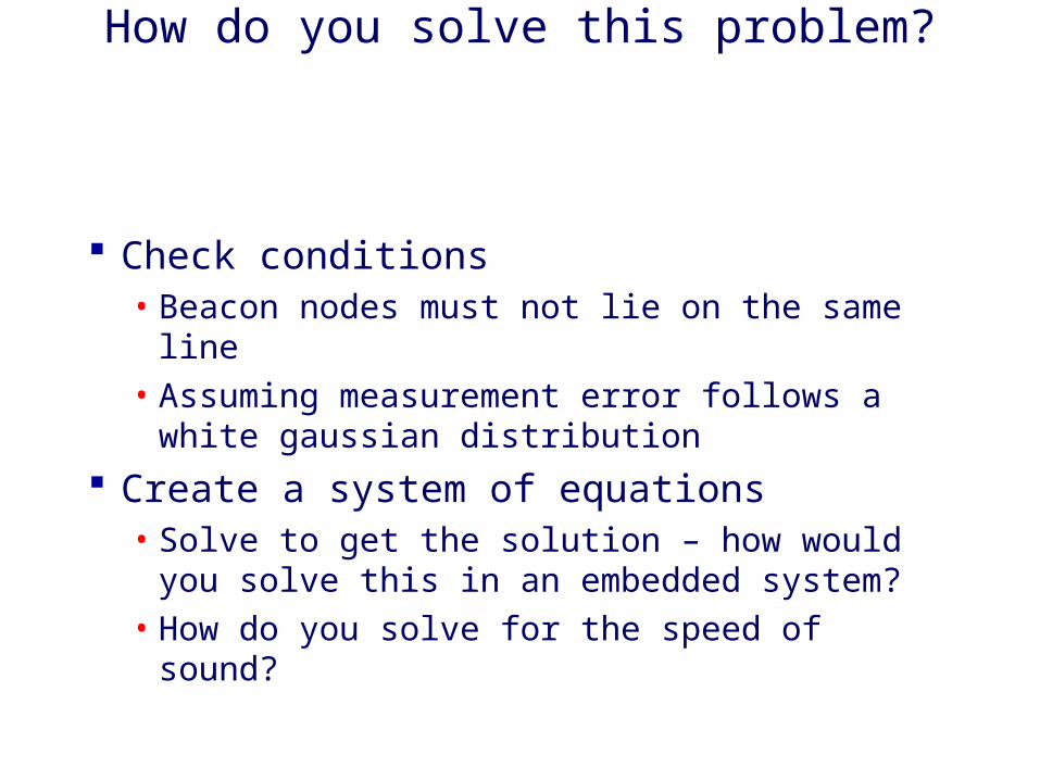
How do you solve this problem?
Check conditions• Beacon nodes must not lie on the same line• Assuming measurement error follows a white
gaussian distribution
Create a system of equations• Solve to get the solution – how would you
solve this in an embedded system?• How do you solve for the speed of sound?
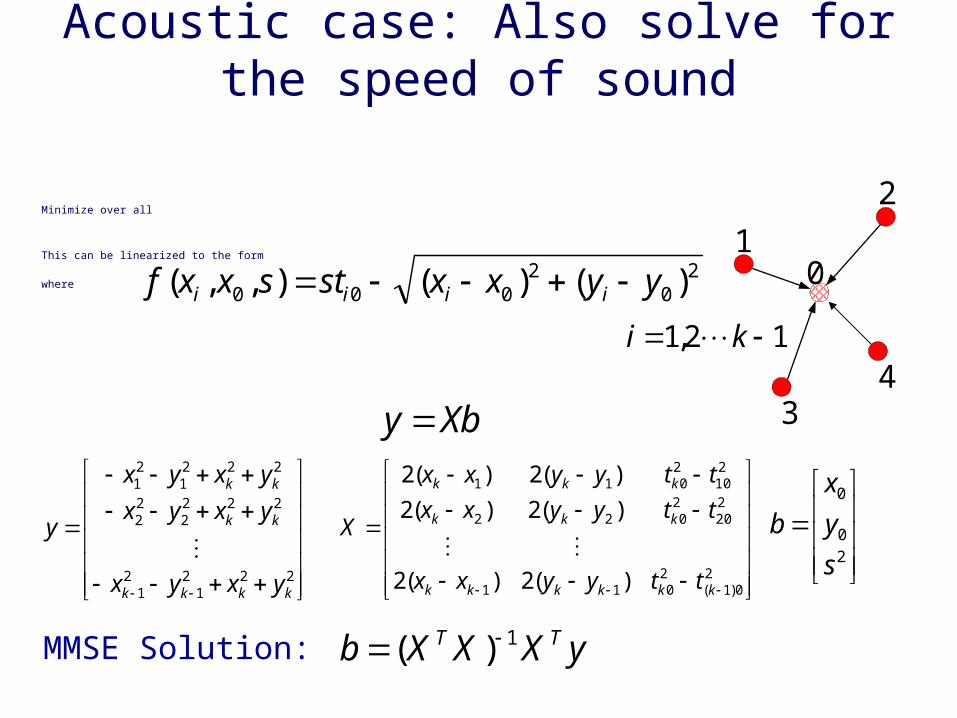
Acoustic case: Also solve for the speed of sound
Minimize over all
This can be linearized to the form
where2
02
000 )()(),,( yyxxstsxxf iiii
Xby
222
12
1
2222
22
2221
21
kkkk
kk
kk
yxyx
yxyx
yxyx
y
2
0)1(2011
220
2022
210
2011
)(2)(2
)(2)(2
)(2)(2
kkkkkk
kkk
kkk
ttyyxx
ttyyxx
ttyyxx
X
20
0
s
y
x
b
1
2
34
0
12,1 ki
yXXXb TT 1)( MMSE Solution:
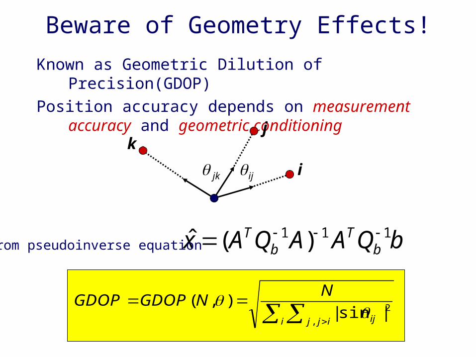
Beware of Geometry Effects!
Known as Geometric Dilution of Precision(GDOP)
Position accuracy depends on measurement accuracy and geometric conditioning
i ijj ij
NNGDOPGDOP
,
2|sin|),(
ijjk i
kj
bQAAQAx bT
bT 111 )(ˆ From pseudoinverse equation
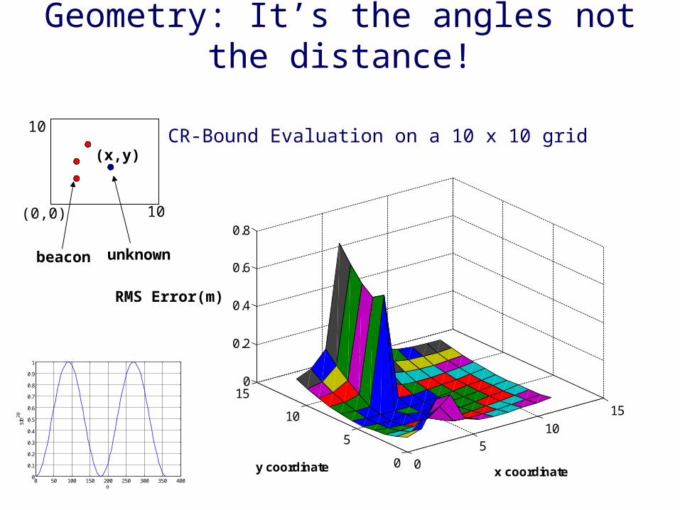
Geometry: It’s the angles not the distance!
0
510
15
0
5
10
150
0.2
0.4
0.6
0.8
x coordinatey coordinate
RMS Error(m)
CR-Bound Evaluation on a 10 x 10 grid
(0,0)
10
10
beacon unknown
(x,y)
0 50 100 150 200 250 300 350 4000
0.1
0.2
0.3
0.4
0.5
0.6
0.7
0.8
0.9
1
sin
2

The Node Localization Problem
Beacon
Unkown Location
Randomly Deployed Sensor Network
Beacon nodes
• Localize nodes in an ad-hoc multihop network• Based on a set of inter-node distance measurements
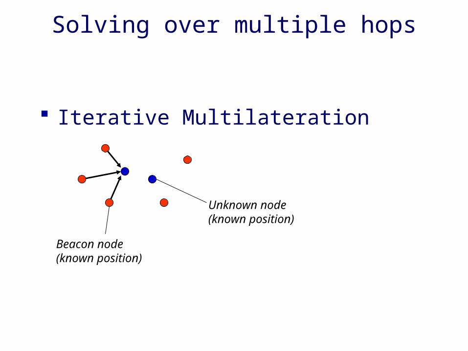
Solving over multiple hops
Iterative Multilateration
Beacon node(known position)
Unknown node(known position)
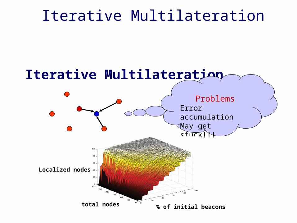
Iterative Multilateration
Iterative Multilateration
ProblemsError accumulationMay get stuck!!!
% of initial beacons
Localized nodes
total nodes
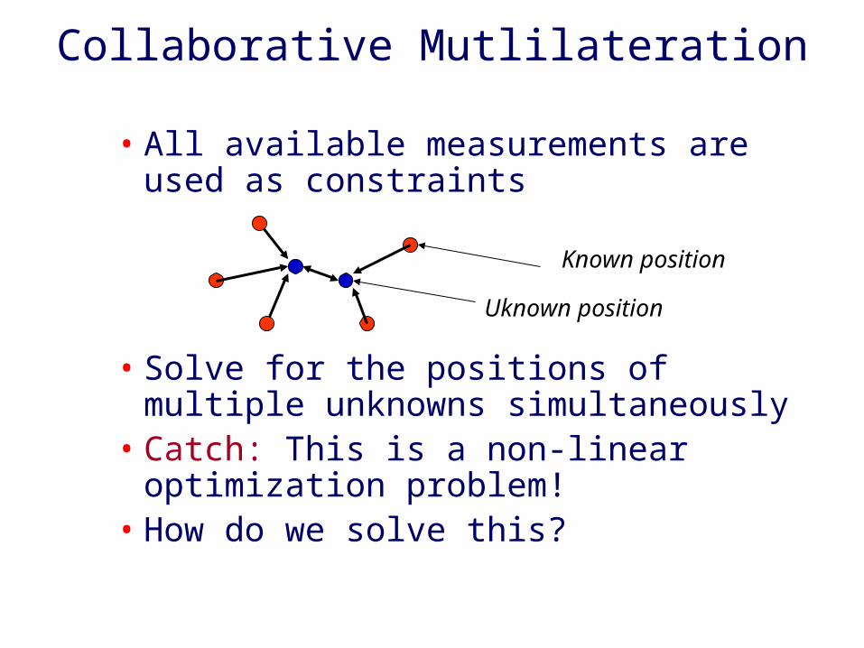
Collaborative Mutlilateration
• All available measurements are used as constraints
• Solve for the positions of multiple unknowns simultaneously
• Catch: This is a non-linear optimization problem!
• How do we solve this?
Known position
Uknown position
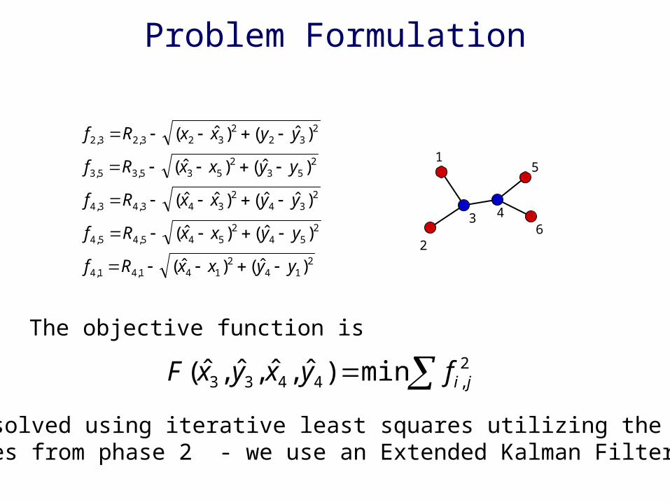
Problem Formulation
214
2141,41,4
254
2545,45,4
234
2343,43,4
253
2535,35,3
232
2323,23,2
)ˆ()ˆ(
)ˆ()ˆ(
)ˆˆ()ˆˆ(
)ˆ()ˆ(
)ˆ()ˆ(
yyxxRf
yyxxRf
yyxxRf
yyxxRf
yyxxRf
2,4433 min)ˆ,ˆ,ˆ,ˆ( jifyxyxF
The objective function is
Can be solved using iterative least squares utilizing the initial Estimates from phase 2 - we use an Extended Kalman Filter
1
2
3 4
5
6
How do we solve this problem?
In an embedded system? Backboard material here… One possible solution would use a Kalman
Filter• This was found to work well in practice, can
“easily” implemented on an embedded processor
[more details see Savvides03]
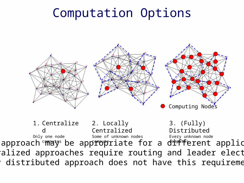
Computation Options
1. CentralizedOnly one node computes
2. Locally Centralized Some of unknown nodes compute
3. (Fully) DistributedEvery unknown node computes
Computing Nodes
• Each approach may be appropriate for a different application• Centralized approaches require routing and leader election• Fully distributed approach does not have this requirement
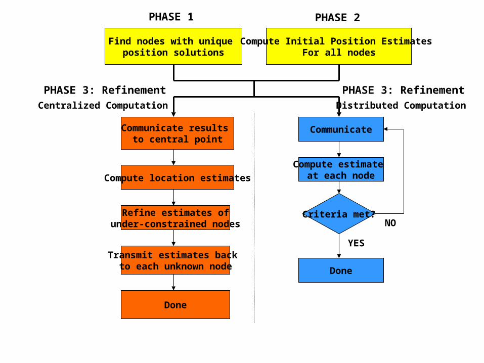
Find nodes with unique position solutions
Compute Initial Position Estimates For all nodes
Compute location estimates
Compute estimate at each node
Communicate
Criteria met?
YES
NO
Communicate results to central point
Transmit estimates back to each unknown node
Refine estimates ofunder-constrained nodes
Done
Done
Centralized Computation Distributed Computation
PHASE 1 PHASE 2
PHASE 3: Refinement PHASE 3: Refinement
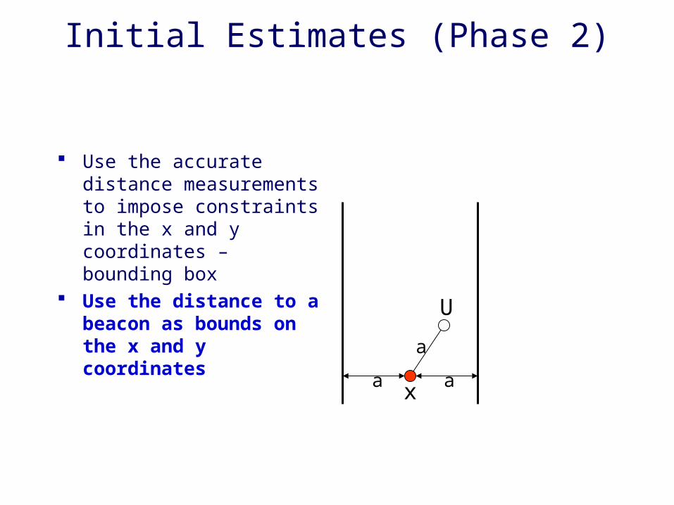
Initial Estimates (Phase 2)
Use the accurate distance measurements to impose constraints in the x and y coordinates – bounding box
Use the distance to a beacon as bounds on the x and y coordinates
a
a ax
U
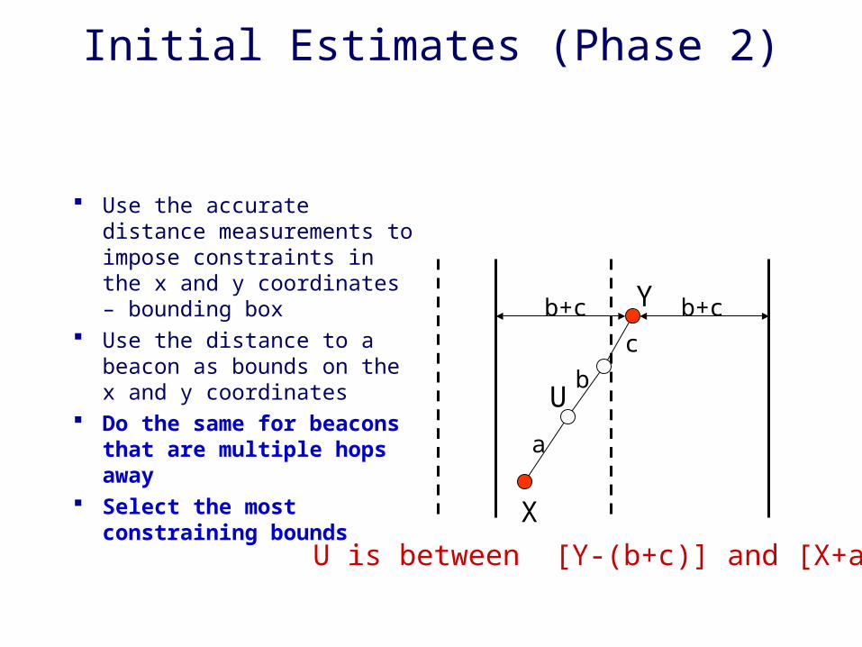
Initial Estimates (Phase 2)
Use the accurate distance measurements to impose constraints in the x and y coordinates – bounding box
Use the distance to a beacon as bounds on the x and y coordinates
Do the same for beacons that are multiple hops away
Select the most constraining bounds
a
b
c
b+c b+c
X
Y
U
U is between [Y-(b+c)] and [X+a]
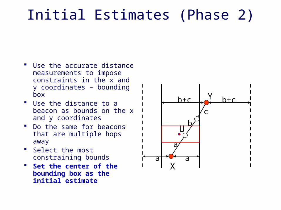
Initial Estimates (Phase 2)
Use the accurate distance measurements to impose constraints in the x and y coordinates – bounding box
Use the distance to a beacon as bounds on the x and y coordinates
Do the same for beacons that are multiple hops away
Select the most constraining bounds
Set the center of the bounding box as the initial estimate
a
a a
b
c
b+c b+c
X
Y
U
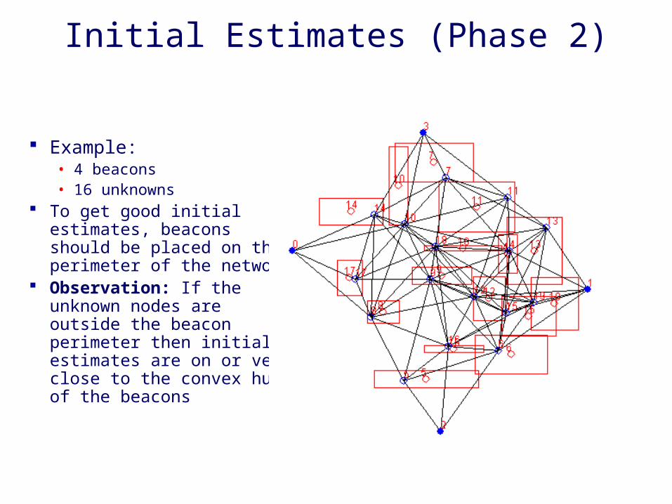
Initial Estimates (Phase 2)
Example:• 4 beacons• 16 unknowns
To get good initial estimates, beacons should be placed on the perimeter of the network
Observation: If the unknown nodes are outside the beacon perimeter then initial estimates are on or very close to the convex hull of the beacons
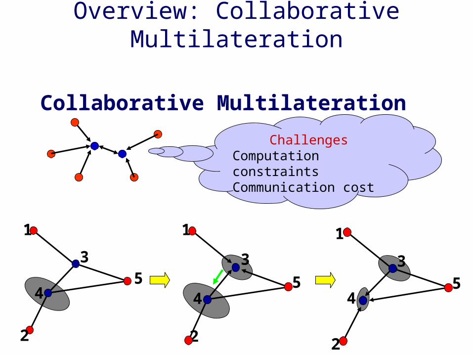
Overview: Collaborative Multilateration
Collaborative Multilateration
ChallengesComputation constraintsCommunication cost
1
2
3
45
2
1
3
45
1
2
3
45
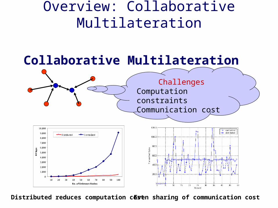
Overview: Collaborative Multilateration
Collaborative Multilateration
ChallengesComputation constraintsCommunication cost
0
1,000
2,000
3,000
4,000
5,000
6,000
7,000
8,000
9,000
10,000
10 20 30 40 50 60 70 80 90 100
No. of Unknown Nodes
MF
lop
s
Distributed Centralized
Distributed reduces computation cost Even sharing of communication cost
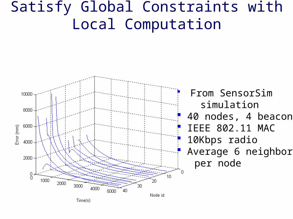
Satisfy Global Constraints with Local Computation
From SensorSim simulation 40 nodes, 4 beacons IEEE 802.11 MAC 10Kbps radio Average 6 neighbors per node
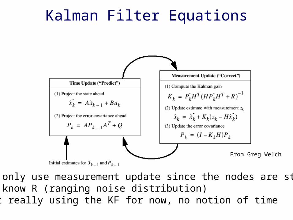
Kalman Filter Equations
From Greg Welch
• We only use measurement update since the nodes are static• We know R (ranging noise distribution)• Not really using the KF for now, no notion of time
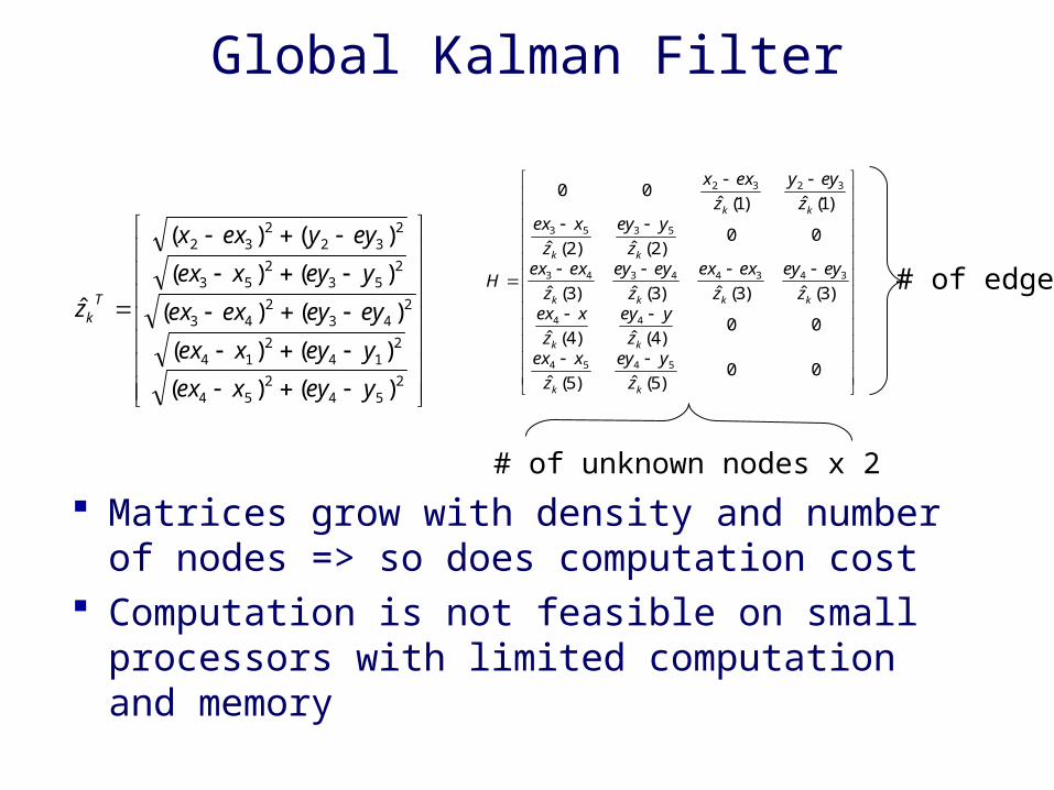
Global Kalman Filter
Matrices grow with density and number of nodes => so does computation cost
Computation is not feasible on small processors with limited computation and memory
00)5(ˆ)5(ˆ
00)4(ˆ)4(ˆ
)3(ˆ)3(ˆ)3(ˆ)3(ˆ
00)2(ˆ)2(ˆ
)1(ˆ)1(ˆ00
5454
44
34344343
5353
3232
kk
kk
kkkk
kk
kk
z
yey
z
xexz
yey
z
xexz
eyey
z
exex
z
eyey
z
exexz
yey
z
xexz
eyy
z
exx
H # of edges
# of unknown nodes x 2
254
254
214
214
243
243
253
253
232
232
)()(
)()(
)()(
)()(
)()(
ˆ
yeyxex
yeyxex
eyeyexex
yeyxex
eyyexx
z Tk
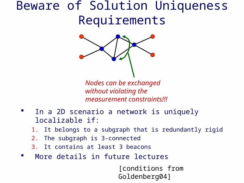
Beware of Solution Uniqueness Requirements
In a 2D scenario a network is uniquely localizable if:1. It belongs to a subgraph that is redundantly rigid
2. The subgraph is 3-connected
3. It contains at least 3 beacons
More details in future lectures
Nodes can be exchanged without violating the measurement constraints!!!
[conditions from Goldenberg04]
Does this solve the problem?
No! Several other challenges Solution depends on
• Problem setupo Infrastructure assisted (beacons), fully ad-hoc & beaconless, hybrid
• Measurement technologyo Distances vs. angles, acoustic vs. rf, connectivity based, proximity basedo The underlying measurement error distribution changes with each technology
The algorithm will also change• Fully distributed computation or centralized• How big is the network and what networking support do you have to solve
the problem?• Mobile vs. static scenarios• Many other possibilities and many different approaches
More next time…
Note
In addition to the slides, you are also responsible for knowing how to solve the problems solved during the blackboard discussion.