Introduction to Learning Classifier Systems Dr. J. Bacardit, Dr. N. Krasnogor G53BIO - Bioinformatics

Introduction to Learning Classifier Systems

Dr. J. Bacardit, Dr. N. Krasnogor

G53BIO - Bioinformatics

Outline

Introduction Machine Learning & Classification Paradigms of LCS Knowledge representations Real-world examples Recent trends Summary

Introduction

Learning Classifier Systems (LCS) are one of the major families of techniques that apply evolutionary computation to machine learning tasks Machine learning: How to construct programs

that automatically learn from experience [Mitchell, 1997]

LCS are almost as ancient as GAs, Holland made one of the first proposals

Introduction

Paradigms of LCS The Pittsburgh approach [Smith, 80] The Michigan approach [Holland & Reitman, 78] The Iterative Rule Learning approach [Venturini,

93] Knowledge representations

All the initial approaches were rule-based In recent years several knowledge

representations have been used in the LCS field: decision trees, synthetic prototypes, etc.

Machine Learning and classification

A more formal definition of machine learning and some examples [Mitchell, 1997] A computer program is said to learn from

experience E with respect to some class of tasks T and performance measure P, if its performance at tasks in T, as measured by P, improves with experience E

How does this definition translate to real life?


A checkers learning problem Task T: playing checkers Performance measure P: percent of

games won against opponents Training experience E: playing practice

games against itself


A handwriting recognition learning problem Task T: recognizing and classifying

handwritten words withing images Performance measure P: percent of

words correctly identified Training experience E: a database of

handwritten words with given classifications


A robot driving learning problem Task T: driving on public four-lane

highways using vision sensors Performance measure P: average

distance traveled before an error (as judged by human overseer)

Training experience E: a sequence of images and steering commands recorded while observing a human driver


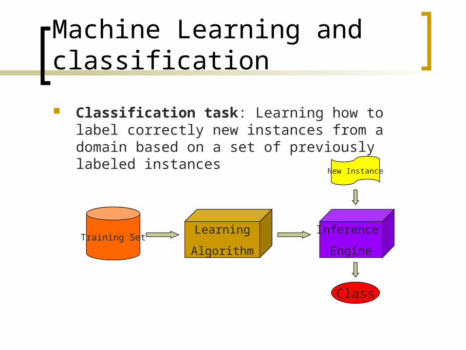
Classification task: Learning how to label correctly new instances from a domain based on a set of previously labeled instances

Training SetLearning

Algorithm

Inference

Engine

New Instance

Class


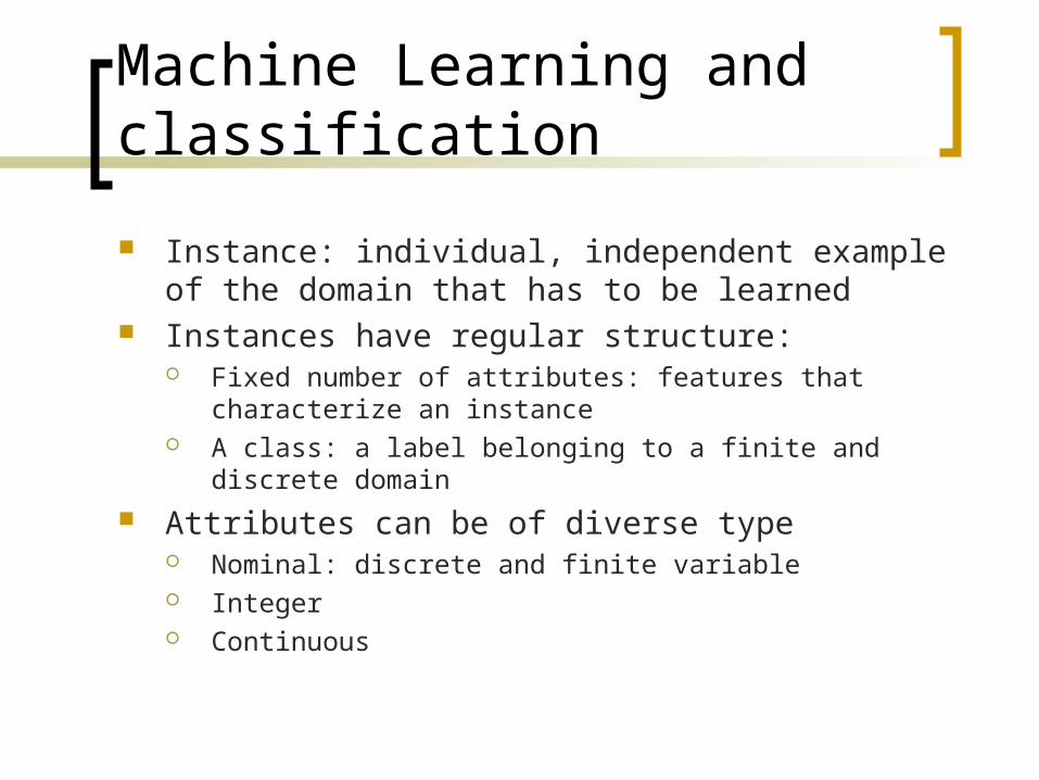
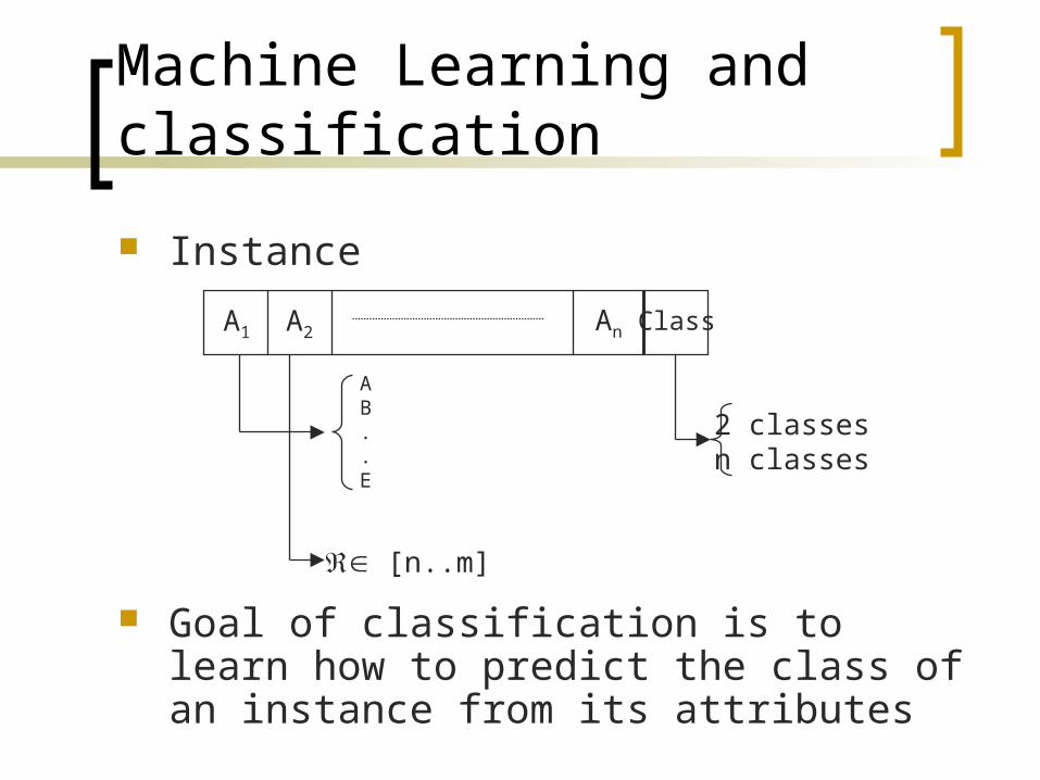
Instance: individual, independent example of the domain that has to be learned

Instances have regular structure: Fixed number of attributes: features that characterize an

instance A class: a label belonging to a finite and discrete domain

Attributes can be of diverse type Nominal: discrete and finite variable Integer Continuous


Instance

Goal of classification is to learn how to predict the class of an instance from its attributes

A1 A2 An Class

AB..E

[n..m]

2 classesn classes


X

Y

0 1

1

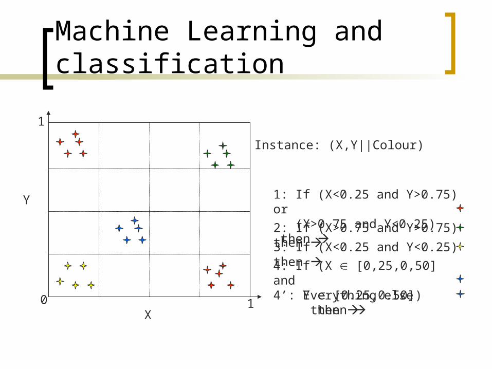
1: If (X<0.25 and Y>0.75) or (X>0.75 and Y<0.25) then

2: If (X>0.75 and Y>0.75) then

3: If (X<0.25 and Y<0.25) then

4: If (X [0,25,0,50] and Y [0.25,0.50]) then

Instance: (X,Y||Colour)

4’: Everything else then

Paradigms of LCS

Paradigms of LCS The Pittsburgh approach [Smith, 80] The Michigan approach [Holland &

Reitman, 78] The Iterative Rule Learning approach

[Venturini, 93]

Paradigms of LCS

The Pittsburgh approach This approach is the closest one to the

standard concept of GA Each individual is a complete solution to

the classification problem Traditionally this means that each

individual is a variable-length set of rules GABIL [De Jong & Spears, 93] is a well-

known representative of this approach

Paradigms of LCS

Pittsburgh approach More than one rule could be used to classify a

given instance Match process: deciding which rule is used in

these cases An usual approach is that individuals are

interpreted as a decision list [Rivest, 87]: an ordered rule set

1 2 3 4 5 6 7 8Instance 1 matches rules 2, 3 and 7 Rule 2 will be usedInstance 2 matches rules 1 and 8 Rule 1 will be usedInstance 3 matches rule 8 Rule 8 will be usedInstance 4 matches no rules Instance 4 will not be classified

Paradigms of LCS

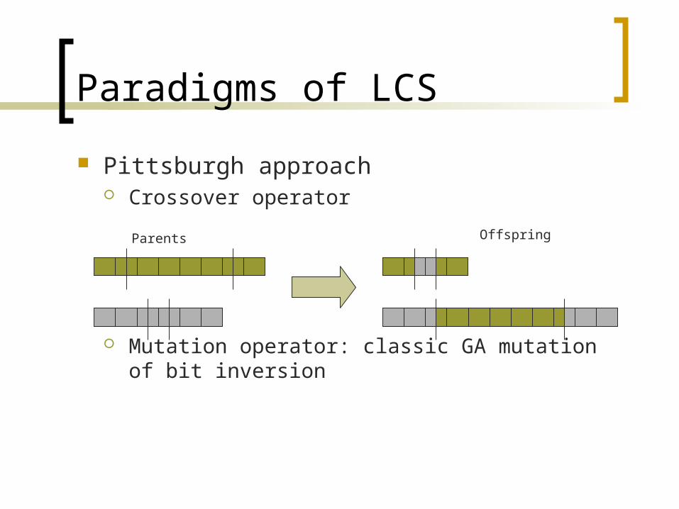
Pittsburgh approach Crossover operator

Mutation operator: classic GA mutation of bit inversion

Parents

Offspring

Paradigms of LCS

Pittsburgh approach Evaluation process of an individual:

NumExamples=0 CorrectExamples=0 For each example in training set

NumExamples++ Determine first rule that matches training example If class of rule is the same as class of instance

CorrectExamples++ Fitness=(CorrectExamples/NumExamples)2

Paradigms of LCS

In the other two approaches each individual is a rule

What happens usually in the evolutionary process of a GA? All individuals converge towards a single

solution Our solution is a set of rules. Therefore we

need some mechanism to guarantee that we generate all of them.

Each approach uses a different method for that

Paradigms of LCS

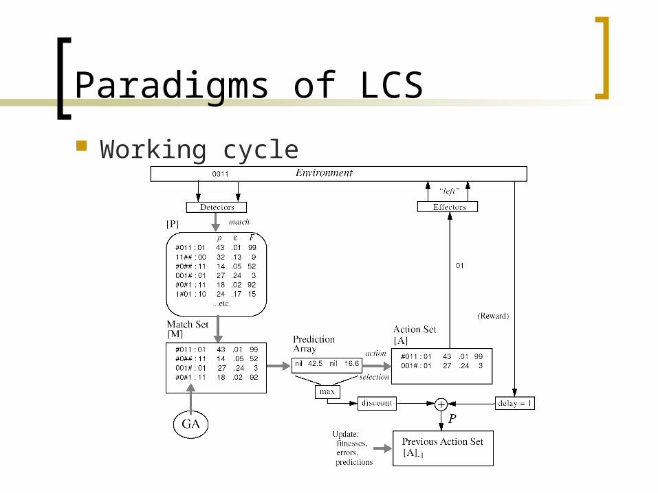
The Michigan approach Each individual (classifier) is a single rule The whole population cooperates to solve the

classification problem A reinforcement learning system is used to

identify the good rules A GA is used to explore the search space for

more rules XCS [Wilson, 95] is the most well-known

Michigan LCS

Paradigms of LCS

The Michigan approach What is Reinforcement Learning?

“a way of programming agents by reward and punishment without needing to specify how the task is to be achieved” [Kaelbling, Littman, & Moore, 96]

Rules will be evaluated example by example, receiving a positive/negative reward

Rule fitness will be update incrementally with this reward

After enough trials, good rules should have high fitness

Paradigms of LCS

Working cycle

Paradigms of LCS

The Iterative Rule Learning approach Each individual is a single rule Individuals compete as in a standard GA

A single GA run generates one rule The GA is run iteratively to learn all rules

that solve the problem Instances already covered by previous

rules are removed from the training set of the next iteration

Paradigms of LCS

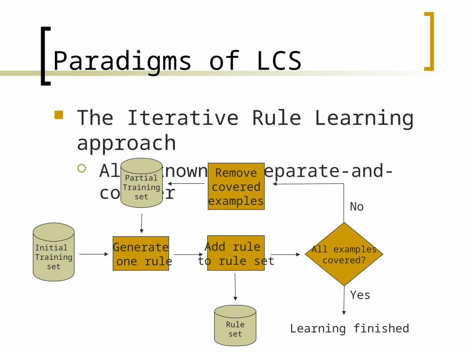
The Iterative Rule Learning approach Also known as separate-and-conquer

Initial Training

set

Generate one rule

Add rule to rule set

Ruleset

All examplescovered?

Removecovered

examples

PartialTraining

set

No

Yes

Learning finished

Paradigms of LCS

The Iterative Rule Learning approach HIDER System [Aguilar, Riquelme & Toro, 03]

1. Input: Examples2. RuleSet = Ø3. While |Examples| > 0

1. Rule = Run GA with Examples2. RuleSet = RuleSet U Rule3. Examples = Examples \ Covered(Rule)

4. EndWhile5. Output: RuleSet

Fitness uses accuracy + generality measure Generality: rule covering as much examples as possible

Knowledge representations

Knowledge representations For nominal attributes

Ternary representation GABIL representation

For real-valued attributes Decision tree Synthetic prototypes Others


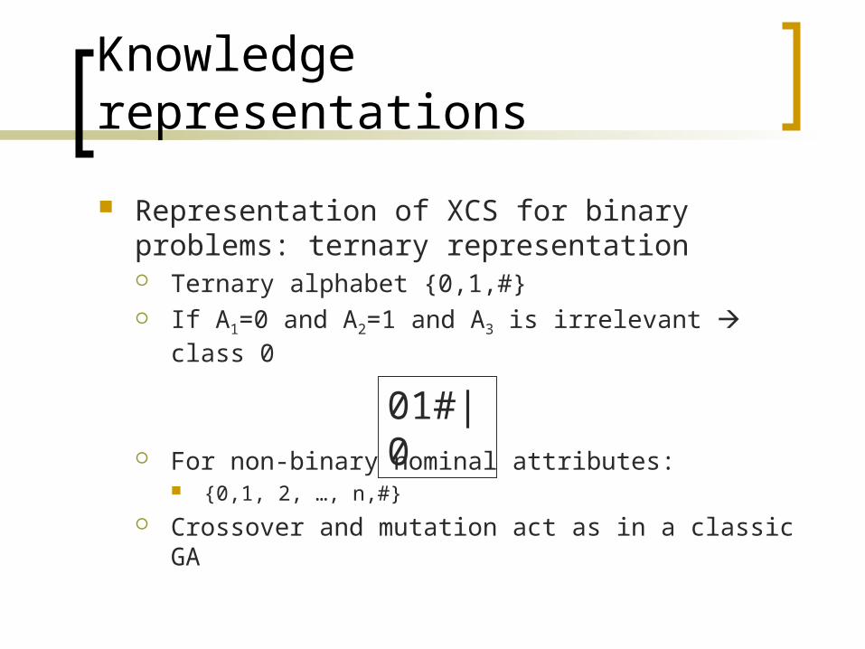
Representation of XCS for binary problems: ternary representation Ternary alphabet {0,1,#} If A1=0 and A2=1 and A3 is irrelevant class 0

For non-binary nominal attributes: {0,1, 2, …, n,#}

Crossover and mutation act as in a classic GA

01#|0


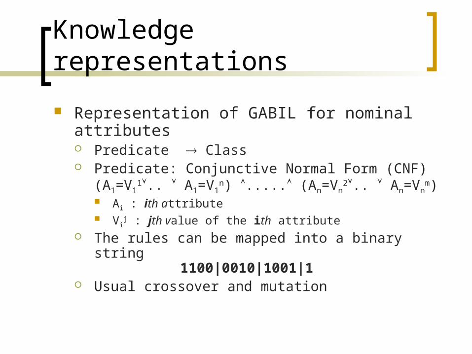
Representation of GABIL for nominal attributes Predicate Class Predicate: Conjunctive Normal Form (CNF)

(A1=V11.. A1=V1

n) ..... (An=Vn2.. An=Vn

m) Ai : ith attribute Vi

j : jth value of the ith attribute The rules can be mapped into a binary string

1100|0010|1001|1 Usual crossover and mutation


Representation of GABIL for nominal attributes 2 Variables:

Sky = {clear, partially cloudy, dark clouds} Pressure = {Low, Medium, High}

2 Classes: {no rain, rain} Rule: If [sky is (partially cloudy or has dark

clouds)] and [pressure is low] then predict rain Genotype: “011|100|1”


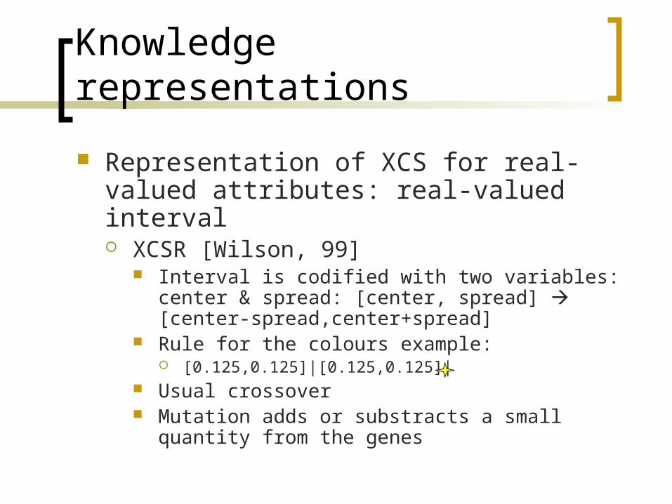
Representation of XCS for real-valued attributes: real-valued interval XCSR [Wilson, 99]

Interval is codified with two variables: center & spread: [center, spread] [center-spread,center+spread]

Rule for the colours example: [0.125,0.125]|[0.125,0.125]|

Usual crossover Mutation adds or substracts a small quantity

from the genes


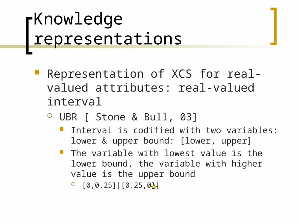
Representation of XCS for real-valued attributes: real-valued interval UBR [ Stone & Bull, 03]

Interval is codified with two variables: lower & upper bound: [lower, upper]

The variable with lowest value is the lower bound, the variable with higher value is the upper bound [0,0.25]|[0.25,0]|


Pittsburgh representations for real-valued attributes: Rule-based: Adaptive Discretization Intervals

(ADI) representation [Bacardit, 04] Intervals in ADI are build using as possible bounds the

cut-points proposed by a discretization algorithm Search bias promotes maximally general intervals Several discretization algorithms are used at the same

time in order to choose correctly the appropiate method for each domain


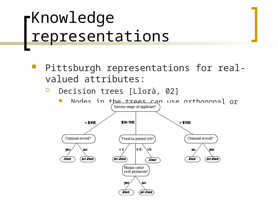
Pittsburgh representations for real-valued attributes: Decision trees [Llorà, 02]

Nodes in the trees can use orthogonal or oblique criteria


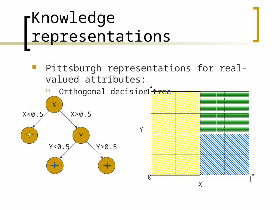
Pittsburgh representations for real-valued attributes: Orthogonal decision tree

XX<0.5

Y

X>0.5

Y<0.5 Y>0.5

X

Y

0 1

1


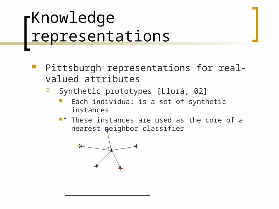
Pittsburgh representations for real-valued attributes Synthetic prototypes [Llorà, 02]

Each individual is a set of synthetic instances These instances are used as the core of a nearest-neighbor

classifier

?

Pittsburgh representations for real-valued attributes Synthetic prototypes

Y

-1 1

1

1. (-0.125,0,yellow)2. (0.125,0,red)3. (0,-0.125,blue)4. (0,0.125,green)

0

Real-world applications

Generating control rules for a fighter aircraft [Smith et. al., 00] Using Michigan LCS Learning aircraft maneuvers Input information:

Airspeed, altitude, aircraft angle, … Actions (classes):

Rudder angle and speed


Predicting the mill temperature (range of temperatures) in a aluminium plate mill [Browne & Bacardit, 04] The Pittsburgh approach was used A press is used to level raw aluminium into a thin

sheet that can be coiled The aluminium temperature should be within

some operational limits Temperature is predicted from around 60 input

sensors


Medical domains: Generation of epidemiologic hypothesis [Holmes, 96] Predicting if a pacient has a disease

based on their degree of exposure to certain factors

In this domain the difference between false positives and false negatives is important

Recent trends

Develop a theoretical framework of the behavior of each kind of LCS These models are intended to allow the

user to adjust the LCS in a principled way to guarantee success

Convert LCS into an engineering tool

Recent trends

New kinds of knowledge representations, specially non-linear ones Making sure that the representation has

enough expressive power to model successfully the domain

Recent trends

Development of exploration mechanism that can go beyond the classic crossover and mutation operators It is known that these classic exploration

mechanisms have limitations, specially in identifying the structure of the problem

If the algorithm learns this structure, it can explore more efficiently and find better solutions

Summary

This talk was a brief overview of the Learning Classifier Systems area: EC techniques applied to Machine Learning

Description of the three main paradigms Pittsburgh Michigan Iterative rule learning

Summary

Description of several knowledge representations Rule based

Nominal attributes Continuous attributes

Decision trees Synthetic prototypes

Summary

Applications to real-world domains Medical Industrial Military

Recent trends Explore better Model the problem better Understand better

Documents

Introduction to Learning Classifier Systems Dr. J. Bacardit, Dr. N. Krasnogor G53BIO - Bioinformatics