Introduction to Information Retrieval - Stanford NLP Group inverted index supports fast nearest-neighbor search for the standard IR setting. However, sometimes we may not be able to

Online edition (c)2009 Cambridge UP

DRAFT! © April 1, 2009 Cambridge University Press. Feedback welcome. 349

16 Flat clustering

Clustering algorithms group a set of documents into subsets or clusters. TheCLUSTER

algorithms’ goal is to create clusters that are coherent internally, but clearlydifferent from each other. In other words, documents within a cluster shouldbe as similar as possible; and documents in one cluster should be as dissimi-lar as possible from documents in other clusters.

0.0 0.5 1.0 1.5 2.0

0.0

0.5

1.0

1.5

2.0

2.5

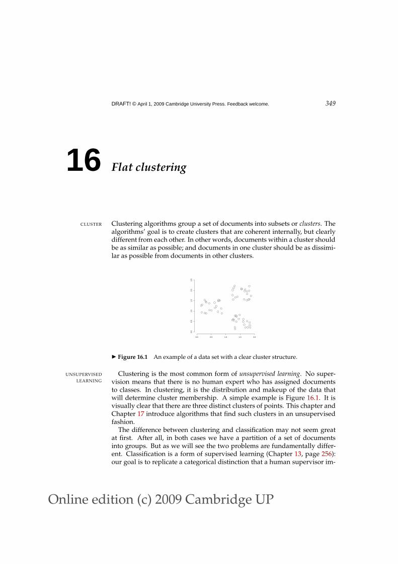
Figure 16.1 An example of a data set with a clear cluster structure.

Clustering is the most common form of unsupervised learning. No super-UNSUPERVISED

LEARNING vision means that there is no human expert who has assigned documentsto classes. In clustering, it is the distribution and makeup of the data thatwill determine cluster membership. A simple example is Figure 16.1. It isvisually clear that there are three distinct clusters of points. This chapter andChapter 17 introduce algorithms that find such clusters in an unsupervisedfashion.

The difference between clustering and classification may not seem greatat first. After all, in both cases we have a partition of a set of documentsinto groups. But as we will see the two problems are fundamentally differ-ent. Classification is a form of supervised learning (Chapter 13, page 256):our goal is to replicate a categorical distinction that a human supervisor im-


350 16 Flat clustering

poses on the data. In unsupervised learning, of which clustering is the mostimportant example, we have no such teacher to guide us.

The key input to a clustering algorithm is the distance measure. In Fig-ure 16.1, the distance measure is distance in the 2D plane. This measure sug-gests three different clusters in the figure. In document clustering, the dis-tance measure is often also Euclidean distance. Different distance measuresgive rise to different clusterings. Thus, the distance measure is an importantmeans by which we can influence the outcome of clustering.

Flat clustering creates a flat set of clusters without any explicit structure thatFLAT CLUSTERING

would relate clusters to each other. Hierarchical clustering creates a hierarchyof clusters and will be covered in Chapter 17. Chapter 17 also addresses thedifficult problem of labeling clusters automatically.

A second important distinction can be made between hard and soft cluster-ing algorithms. Hard clustering computes a hard assignment – each documentHARD CLUSTERING

is a member of exactly one cluster. The assignment of soft clustering algo-SOFT CLUSTERING

rithms is soft – a document’s assignment is a distribution over all clusters.In a soft assignment, a document has fractional membership in several clus-ters. Latent semantic indexing, a form of dimensionality reduction, is a softclustering algorithm (Chapter 18, page 417).

This chapter motivates the use of clustering in information retrieval byintroducing a number of applications (Section 16.1), defines the problemwe are trying to solve in clustering (Section 16.2) and discusses measuresfor evaluating cluster quality (Section 16.3). It then describes two flat clus-tering algorithms, K-means (Section 16.4), a hard clustering algorithm, andthe Expectation-Maximization (or EM) algorithm (Section 16.5), a soft clus-tering algorithm. K-means is perhaps the most widely used flat clusteringalgorithm due to its simplicity and efficiency. The EM algorithm is a gen-eralization of K-means and can be applied to a large variety of documentrepresentations and distributions.

16.1 Clustering in information retrieval

The cluster hypothesis states the fundamental assumption we make when us-CLUSTER HYPOTHESIS

ing clustering in information retrieval.

Cluster hypothesis. Documents in the same cluster behave similarlywith respect to relevance to information needs.

The hypothesis states that if there is a document from a cluster that is rele-vant to a search request, then it is likely that other documents from the samecluster are also relevant. This is because clustering puts together documentsthat share many terms. The cluster hypothesis essentially is the contiguity


16.1 Clustering in information retrieval 351

Application What is Benefit Exampleclustered?

Search result clustering searchresults

more effective informationpresentation to user

Figure 16.2

Scatter-Gather (subsets of)collection

alternative user interface:“search without typing”

Figure 16.3

Collection clustering collection effective information pre-sentation for exploratorybrowsing

McKeown et al. (2002),http://news.google.com

Language modeling collection increased precision and/orrecall Liu and Croft (2004)

Cluster-based retrieval collection higher efficiency: fastersearch Salton (1971a)

Table 16.1 Some applications of clustering in information retrieval.

hypothesis in Chapter 14 (page 289). In both cases, we posit that similardocuments behave similarly with respect to relevance.

Table 16.1 shows some of the main applications of clustering in informa-tion retrieval. They differ in the set of documents that they cluster – searchresults, collection or subsets of the collection – and the aspect of an informa-tion retrieval system they try to improve – user experience, user interface,effectiveness or efficiency of the search system. But they are all based on thebasic assumption stated by the cluster hypothesis.

The first application mentioned in Table 16.1 is search result clustering whereSEARCH RESULT

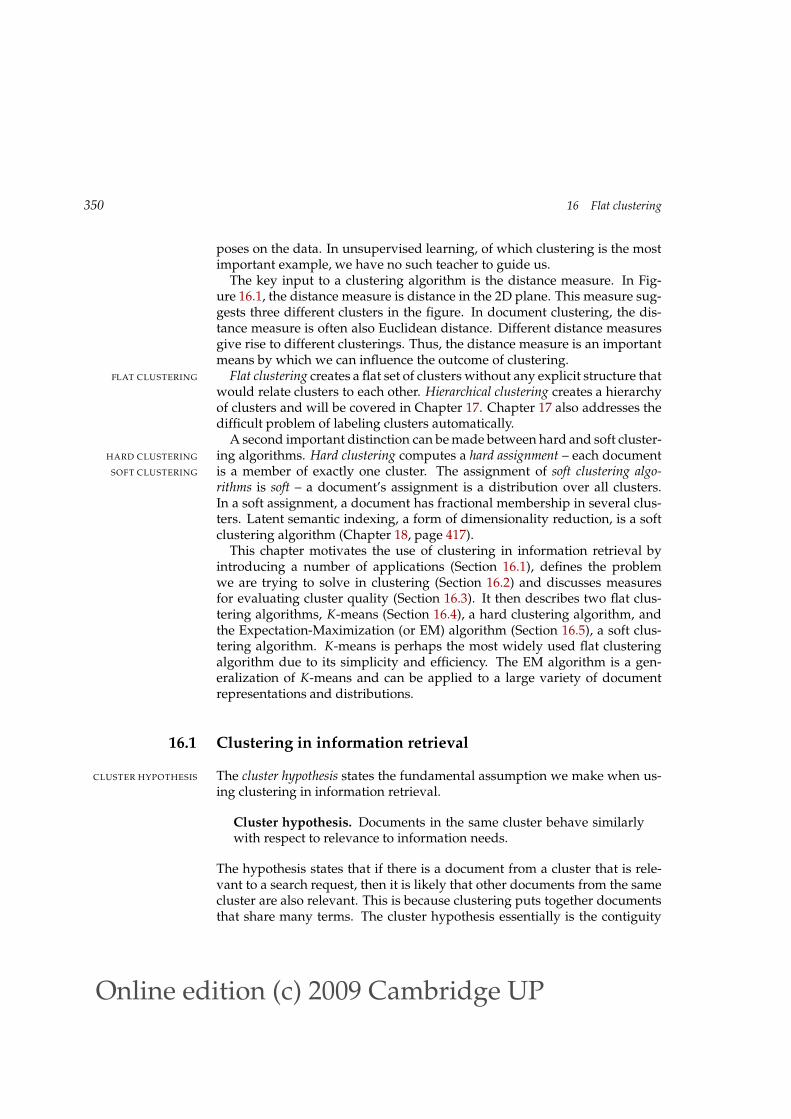
CLUSTERING by search results we mean the documents that were returned in response toa query. The default presentation of search results in information retrieval isa simple list. Users scan the list from top to bottom until they have foundthe information they are looking for. Instead, search result clustering clus-ters the search results, so that similar documents appear together. It is ofteneasier to scan a few coherent groups than many individual documents. Thisis particularly useful if a search term has different word senses. The examplein Figure 16.2 is jaguar. Three frequent senses on the web refer to the car, theanimal and an Apple operating system. The Clustered Results panel returnedby the Vivísimo search engine (http://vivisimo.com) can be a more effective userinterface for understanding what is in the search results than a simple list ofdocuments.

A better user interface is also the goal of Scatter-Gather, the second ap-SCATTER-GATHER

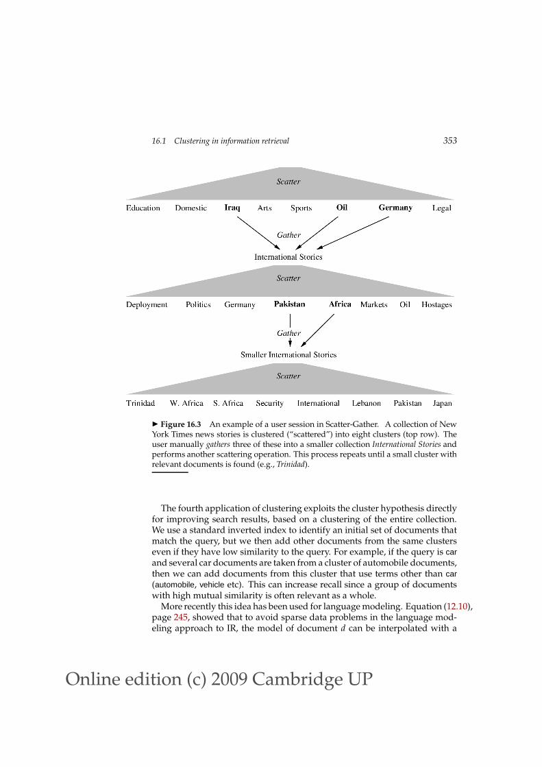
plication in Table 16.1. Scatter-Gather clusters the whole collection to getgroups of documents that the user can select or gather. The selected groupsare merged and the resulting set is again clustered. This process is repeateduntil a cluster of interest is found. An example is shown in Figure 16.3.



Figure 16.2 Clustering of search results to improve recall. None of the top hitscover the animal sense of jaguar, but users can easily access it by clicking on the catcluster in the Clustered Results panel on the left (third arrow from the top).

Automatically generated clusters like those in Figure 16.3 are not as neatlyorganized as a manually constructed hierarchical tree like the Open Direc-tory at http://dmoz.org. Also, finding descriptive labels for clusters automati-cally is a difficult problem (Section 17.7, page 396). But cluster-based navi-gation is an interesting alternative to keyword searching, the standard infor-mation retrieval paradigm. This is especially true in scenarios where usersprefer browsing over searching because they are unsure about which searchterms to use.

As an alternative to the user-mediated iterative clustering in Scatter-Gather,we can also compute a static hierarchical clustering of a collection that isnot influenced by user interactions (“Collection clustering” in Table 16.1).Google News and its precursor, the Columbia NewsBlaster system, are ex-amples of this approach. In the case of news, we need to frequently recom-pute the clustering to make sure that users can access the latest breakingstories. Clustering is well suited for access to a collection of news storiessince news reading is not really search, but rather a process of selecting asubset of stories about recent events.


16.1 Clustering in information retrieval 353

Figure 16.3 An example of a user session in Scatter-Gather. A collection of NewYork Times news stories is clustered (“scattered”) into eight clusters (top row). Theuser manually gathers three of these into a smaller collection International Stories andperforms another scattering operation. This process repeats until a small cluster withrelevant documents is found (e.g., Trinidad).

The fourth application of clustering exploits the cluster hypothesis directlyfor improving search results, based on a clustering of the entire collection.We use a standard inverted index to identify an initial set of documents thatmatch the query, but we then add other documents from the same clusterseven if they have low similarity to the query. For example, if the query is carand several car documents are taken from a cluster of automobile documents,then we can add documents from this cluster that use terms other than car(automobile, vehicle etc). This can increase recall since a group of documentswith high mutual similarity is often relevant as a whole.

More recently this idea has been used for language modeling. Equation (12.10),page 245, showed that to avoid sparse data problems in the language mod-eling approach to IR, the model of document d can be interpolated with a



collection model. But the collection contains many documents with termsuntypical of d. By replacing the collection model with a model derived fromd’s cluster, we get more accurate estimates of the occurrence probabilities ofterms in d.

Clustering can also speed up search. As we saw in Section 6.3.2 (page 123)search in the vector space model amounts to finding the nearest neighborsto the query. The inverted index supports fast nearest-neighbor search forthe standard IR setting. However, sometimes we may not be able to use aninverted index efficiently, e.g., in latent semantic indexing (Chapter 18). Insuch cases, we could compute the similarity of the query to every document,but this is slow. The cluster hypothesis offers an alternative: Find the clus-ters that are closest to the query and only consider documents from theseclusters. Within this much smaller set, we can compute similarities exhaus-tively and rank documents in the usual way. Since there are many fewerclusters than documents, finding the closest cluster is fast; and since the doc-uments matching a query are all similar to each other, they tend to be inthe same clusters. While this algorithm is inexact, the expected decrease insearch quality is small. This is essentially the application of clustering thatwas covered in Section 7.1.6 (page 141).

? Exercise 16.1

Define two documents as similar if they have at least two proper names like Clintonor Sarkozy in common. Give an example of an information need and two documents,for which the cluster hypothesis does not hold for this notion of similarity.

Exercise 16.2

Make up a simple one-dimensional example (i.e. points on a line) with two clusterswhere the inexactness of cluster-based retrieval shows up. In your example, retriev-ing clusters close to the query should do worse than direct nearest neighbor search.

16.2 Problem statement

We can define the goal in hard flat clustering as follows. Given (i) a set ofdocuments D = d1, . . . , dN, (ii) a desired number of clusters K, and (iii)an objective function that evaluates the quality of a clustering, we want toOBJECTIVE FUNCTION

compute an assignment γ : D → 1, . . . , K that minimizes (or, in othercases, maximizes) the objective function. In most cases, we also demand thatγ is surjective, i.e., that none of the K clusters is empty.

The objective function is often defined in terms of similarity or distancebetween documents. Below, we will see that the objective in K-means clus-tering is to minimize the average distance between documents and their cen-troids or, equivalently, to maximize the similarity between documents andtheir centroids. The discussion of similarity measures and distance metrics


16.2 Problem statement 355

in Chapter 14 (page 291) also applies to this chapter. As in Chapter 14, we useboth similarity and distance to talk about relatedness between documents.

For documents, the type of similarity we want is usually topic similarityor high values on the same dimensions in the vector space model. For exam-ple, documents about China have high values on dimensions like Chinese,Beijing, and Mao whereas documents about the UK tend to have high valuesfor London, Britain and Queen. We approximate topic similarity with cosinesimilarity or Euclidean distance in vector space (Chapter 6). If we intend tocapture similarity of a type other than topic, for example, similarity of lan-guage, then a different representation may be appropriate. When computingtopic similarity, stop words can be safely ignored, but they are importantcues for separating clusters of English (in which the occurs frequently and lainfrequently) and French documents (in which the occurs infrequently and lafrequently).

A note on terminology. An alternative definition of hard clustering is thata document can be a full member of more than one cluster. Partitional clus-PARTITIONAL

CLUSTERING tering always refers to a clustering where each document belongs to exactlyone cluster. (But in a partitional hierarchical clustering (Chapter 17) all mem-bers of a cluster are of course also members of its parent.) On the definitionof hard clustering that permits multiple membership, the difference betweensoft clustering and hard clustering is that membership values in hard clus-tering are either 0 or 1, whereas they can take on any non-negative value insoft clustering.

Some researchers distinguish between exhaustive clusterings that assignEXHAUSTIVE

each document to a cluster and non-exhaustive clusterings, in which somedocuments will be assigned to no cluster. Non-exhaustive clusterings inwhich each document is a member of either no cluster or one cluster arecalled exclusive. We define clustering to be exhaustive in this book.EXCLUSIVE

16.2.1 Cardinality – the number of clusters

A difficult issue in clustering is determining the number of clusters or cardi-CARDINALITY

nality of a clustering, which we denote by K. Often K is nothing more thana good guess based on experience or domain knowledge. But for K-means,we will also introduce a heuristic method for choosing K and an attempt toincorporate the selection of K into the objective function. Sometimes the ap-plication puts constraints on the range of K. For example, the Scatter-Gatherinterface in Figure 16.3 could not display more than about K = 10 clustersper layer because of the size and resolution of computer monitors in the early1990s.

Since our goal is to optimize an objective function, clustering is essentially



a search problem. The brute force solution would be to enumerate all pos-sible clusterings and pick the best. However, there are exponentially manypartitions, so this approach is not feasible.1 For this reason, most flat clus-tering algorithms refine an initial partitioning iteratively. If the search startsat an unfavorable initial point, we may miss the global optimum. Finding agood starting point is therefore another important problem we have to solvein flat clustering.

16.3 Evaluation of clustering

Typical objective functions in clustering formalize the goal of attaining highintra-cluster similarity (documents within a cluster are similar) and low inter-cluster similarity (documents from different clusters are dissimilar). This isan internal criterion for the quality of a clustering. But good scores on anINTERNAL CRITERION

OF QUALITY internal criterion do not necessarily translate into good effectiveness in anapplication. An alternative to internal criteria is direct evaluation in the ap-plication of interest. For search result clustering, we may want to measurethe time it takes users to find an answer with different clustering algorithms.This is the most direct evaluation, but it is expensive, especially if large userstudies are necessary.

As a surrogate for user judgments, we can use a set of classes in an evalua-tion benchmark or gold standard (see Section 8.5, page 164, and Section 13.6,page 279). The gold standard is ideally produced by human judges with agood level of inter-judge agreement (see Chapter 8, page 152). We can thencompute an external criterion that evaluates how well the clustering matchesEXTERNAL CRITERION

OF QUALITY the gold standard classes. For example, we may want to say that the opti-mal clustering of the search results for jaguar in Figure 16.2 consists of threeclasses corresponding to the three senses car, animal, and operating system.In this type of evaluation, we only use the partition provided by the goldstandard, not the class labels.

This section introduces four external criteria of clustering quality. Purity isa simple and transparent evaluation measure. Normalized mutual informationcan be information-theoretically interpreted. The Rand index penalizes bothfalse positive and false negative decisions during clustering. The F measurein addition supports differential weighting of these two types of errors.

To compute purity, each cluster is assigned to the class which is most fre-PURITY

quent in the cluster, and then the accuracy of this assignment is measuredby counting the number of correctly assigned documents and dividing by N.

1. An upper bound on the number of clusterings is KN/K!. The exact number of differentpartitions of N documents into K clusters is the Stirling number of the second kind. Seehttp://mathworld.wolfram.com/StirlingNumberoftheSecondKind.html or Comtet (1974).


16.3 Evaluation of clustering 357

x

o

x x

x

x

o

x

o

o ⋄o x

⋄ ⋄

⋄

x

cluster 1 cluster 2 cluster 3

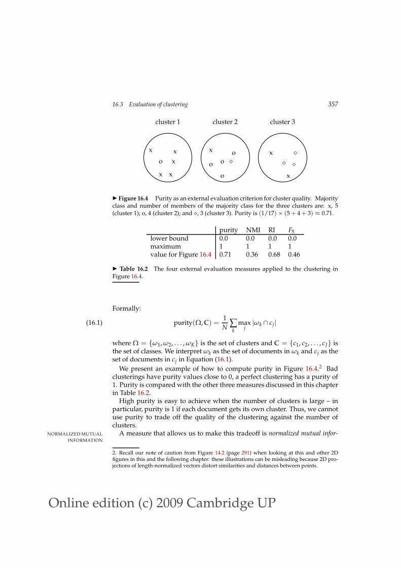
Figure 16.4 Purity as an external evaluation criterion for cluster quality. Majorityclass and number of members of the majority class for the three clusters are: x, 5(cluster 1); o, 4 (cluster 2); and ⋄, 3 (cluster 3). Purity is (1/17)× (5 + 4 + 3) ≈ 0.71.

purity NMI RI F5

lower bound 0.0 0.0 0.0 0.0maximum 1 1 1 1value for Figure 16.4 0.71 0.36 0.68 0.46

Table 16.2 The four external evaluation measures applied to the clustering inFigure 16.4.

Formally:

purity(Ω, C) =1

N ∑k

maxj|ωk ∩ cj|(16.1)

where Ω = ω1, ω2, . . . , ωK is the set of clusters and C = c1, c2, . . . , cJ isthe set of classes. We interpret ωk as the set of documents in ωk and cj as theset of documents in cj in Equation (16.1).

We present an example of how to compute purity in Figure 16.4.2 Badclusterings have purity values close to 0, a perfect clustering has a purity of1. Purity is compared with the other three measures discussed in this chapterin Table 16.2.

High purity is easy to achieve when the number of clusters is large – inparticular, purity is 1 if each document gets its own cluster. Thus, we cannotuse purity to trade off the quality of the clustering against the number ofclusters.

A measure that allows us to make this tradeoff is normalized mutual infor-NORMALIZED MUTUAL

INFORMATION

2. Recall our note of caution from Figure 14.2 (page 291) when looking at this and other 2Dfigures in this and the following chapter: these illustrations can be misleading because 2D pro-jections of length-normalized vectors distort similarities and distances between points.



mation or NMI:

NMI(Ω, C) =I(Ω; C)

[H(Ω) + H(C)]/2(16.2)

I is mutual information (cf. Chapter 13, page 272):

I(Ω; C) = ∑k

∑j

P(ωk ∩ cj) logP(ωk ∩ cj)

P(ωk)P(cj)(16.3)

= ∑k

∑j

|ωk ∩ cj|

Nlog

N|ωk ∩ cj|

|ωk||cj|(16.4)

where P(ωk), P(cj), and P(ωk ∩ cj) are the probabilities of a document beingin cluster ωk, class cj, and in the intersection of ωk and cj, respectively. Equa-tion (16.4) is equivalent to Equation (16.3) for maximum likelihood estimatesof the probabilities (i.e., the estimate of each probability is the correspondingrelative frequency).

H is entropy as defined in Chapter 5 (page 99):

H(Ω) = −∑k

P(ωk) log P(ωk)(16.5)

= −∑k

|ωk|

Nlog|ωk|

N(16.6)

where, again, the second equation is based on maximum likelihood estimatesof the probabilities.

I(Ω; C) in Equation (16.3) measures the amount of information by whichour knowledge about the classes increases when we are told what the clustersare. The minimum of I(Ω; C) is 0 if the clustering is random with respect toclass membership. In that case, knowing that a document is in a particularcluster does not give us any new information about what its class might be.Maximum mutual information is reached for a clustering Ωexact that perfectlyrecreates the classes – but also if clusters in Ωexact are further subdivided intosmaller clusters (Exercise 16.7). In particular, a clustering with K = N one-document clusters has maximum MI. So MI has the same problem as purity:it does not penalize large cardinalities and thus does not formalize our biasthat, other things being equal, fewer clusters are better.

The normalization by the denominator [H(Ω)+ H(C)]/2 in Equation (16.2)fixes this problem since entropy tends to increase with the number of clus-ters. For example, H(Ω) reaches its maximum log N for K = N, which en-sures that NMI is low for K = N. Because NMI is normalized, we can useit to compare clusterings with different numbers of clusters. The particularform of the denominator is chosen because [H(Ω) + H(C)]/2 is a tight upperbound on I(Ω; C) (Exercise 16.8). Thus, NMI is always a number between 0and 1.


16.3 Evaluation of clustering 359

An alternative to this information-theoretic interpretation of clustering isto view it as a series of decisions, one for each of the N(N − 1)/2 pairs ofdocuments in the collection. We want to assign two documents to the samecluster if and only if they are similar. A true positive (TP) decision assignstwo similar documents to the same cluster, a true negative (TN) decision as-signs two dissimilar documents to different clusters. There are two typesof errors we can commit. A false positive (FP) decision assigns two dissim-ilar documents to the same cluster. A false negative (FN) decision assignstwo similar documents to different clusters. The Rand index (RI) measuresRAND INDEX

RI the percentage of decisions that are correct. That is, it is simply accuracy(Section 8.3, page 155).

RI =TP + TN

TP + FP + FN + TN

As an example, we compute RI for Figure 16.4. We first compute TP + FP.The three clusters contain 6, 6, and 5 points, respectively, so the total numberof “positives” or pairs of documents that are in the same cluster is:

TP + FP =

(62

)+

(62

)+

(52

)= 40

Of these, the x pairs in cluster 1, the o pairs in cluster 2, the ⋄ pairs in cluster 3,and the x pair in cluster 3 are true positives:

TP =

(52

)+

(42

)+

(32

)+

(22

)= 20

Thus, FP = 40− 20 = 20.FN and TN are computed similarly, resulting in the following contingency

table:

Same cluster Different clustersSame class TP = 20 FN = 24Different classes FP = 20 TN = 72

RI is then (20 + 72)/(20 + 20 + 24 + 72) ≈ 0.68.The Rand index gives equal weight to false positives and false negatives.

Separating similar documents is sometimes worse than putting pairs of dis-similar documents in the same cluster. We can use the F measure (Section 8.3,F MEASURE

page 154) to penalize false negatives more strongly than false positives byselecting a value β > 1, thus giving more weight to recall.

P =TP

TP + FPR =

TP

TP + FNFβ =

(β2 + 1)PR

β2P + R



Based on the numbers in the contingency table, P = 20/40 = 0.5 and R =20/44 ≈ 0.455. This gives us F1 ≈ 0.48 for β = 1 and F5 ≈ 0.456 for β = 5.In information retrieval, evaluating clustering with F has the advantage thatthe measure is already familiar to the research community.

? Exercise 16.3

Replace every point d in Figure 16.4 with two identical copies of d in the same class.(i) Is it less difficult, equally difficult or more difficult to cluster this set of 34 pointsas opposed to the 17 points in Figure 16.4? (ii) Compute purity, NMI, RI, and F5 forthe clustering with 34 points. Which measures increase and which stay the same afterdoubling the number of points? (iii) Given your assessment in (i) and the results in(ii), which measures are best suited to compare the quality of the two clusterings?

16.4 K-means

K-means is the most important flat clustering algorithm. Its objective is tominimize the average squared Euclidean distance (Chapter 6, page 131) ofdocuments from their cluster centers where a cluster center is defined as themean or centroid ~µ of the documents in a cluster ω:CENTROID

~µ(ω) =1

|ω| ∑~x∈ω

~x

The definition assumes that documents are represented as length-normalizedvectors in a real-valued space in the familiar way. We used centroids for Roc-chio classification in Chapter 14 (page 292). They play a similar role here.The ideal cluster in K-means is a sphere with the centroid as its center ofgravity. Ideally, the clusters should not overlap. Our desiderata for classesin Rocchio classification were the same. The difference is that we have no la-beled training set in clustering for which we know which documents shouldbe in the same cluster.

A measure of how well the centroids represent the members of their clus-ters is the residual sum of squares or RSS, the squared distance of each vectorRESIDUAL SUM OF

SQUARES from its centroid summed over all vectors:

RSSk = ∑~x∈ωk

|~x−~µ(ωk)|2

RSS =K

∑k=1

RSSk(16.7)

RSS is the objective function in K-means and our goal is to minimize it. SinceN is fixed, minimizing RSS is equivalent to minimizing the average squareddistance, a measure of how well centroids represent their documents.


16.4 K-means 361

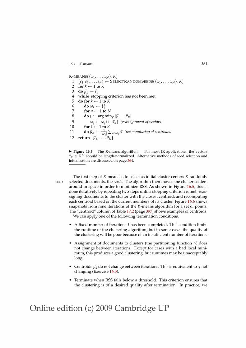
K-MEANS(~x1, . . . ,~xN, K)1 (~s1,~s2, . . . ,~sK)← SELECTRANDOMSEEDS(~x1, . . . ,~xN, K)2 for k← 1 to K3 do ~µk ←~sk

4 while stopping criterion has not been met5 do for k← 1 to K6 do ωk ← 7 for n← 1 to N8 do j← arg minj′ |~µj′ −~xn|

9 ωj ← ωj ∪ ~xn (reassignment of vectors)10 for k← 1 to K11 do ~µk ←

1|ωk|

∑~x∈ωk~x (recomputation of centroids)

12 return ~µ1, . . . ,~µK

Figure 16.5 The K-means algorithm. For most IR applications, the vectors~xn ∈ RM should be length-normalized. Alternative methods of seed selection andinitialization are discussed on page 364.

The first step of K-means is to select as initial cluster centers K randomlyselected documents, the seeds. The algorithm then moves the cluster centersSEED

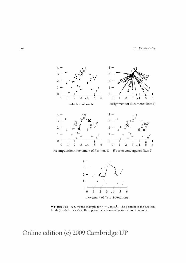
around in space in order to minimize RSS. As shown in Figure 16.5, this isdone iteratively by repeating two steps until a stopping criterion is met: reas-signing documents to the cluster with the closest centroid; and recomputingeach centroid based on the current members of its cluster. Figure 16.6 showssnapshots from nine iterations of the K-means algorithm for a set of points.The “centroid” column of Table 17.2 (page 397) shows examples of centroids.

We can apply one of the following termination conditions.

• A fixed number of iterations I has been completed. This condition limitsthe runtime of the clustering algorithm, but in some cases the quality ofthe clustering will be poor because of an insufficient number of iterations.

• Assignment of documents to clusters (the partitioning function γ) doesnot change between iterations. Except for cases with a bad local mini-mum, this produces a good clustering, but runtimes may be unacceptablylong.

• Centroids ~µk do not change between iterations. This is equivalent to γ notchanging (Exercise 16.5).

• Terminate when RSS falls below a threshold. This criterion ensures thatthe clustering is of a desired quality after termination. In practice, we



0 1 2 3 4 5 60

1

2

3

4

b

b

b

b

b

b

b

b

b

b

b

b

b

b

bb

b

bb

b

bb

bb

b

b

b

b

b

b

b b

b

b

b

b

b

b

b

b

××

selection of seeds

0 1 2 3 4 5 60

1

2

3

4

b

b

b

b

b

b

b

b

b

b

b

b

b

b

bb

b

bb

b

bb

bb

b

b

b

b

b

b

b b

b

b

b

b

b

b

b

b

××

assignment of documents (iter. 1)

0 1 2 3 4 5 60

1

2

3

4

++

+

+

+

+

+

+

++

+

oo

+

o+

+

++

+++ + o

+

+

o

+

+ +

+ o

o

+

o

+

+o+

o

×××

×

recomputation/movement of ~µ’s (iter. 1)

0 1 2 3 4 5 60

1

2

3

4

++

+

+

+

+

+

+

++

+

++

+

o+

+

++

+o+ o o

o

o

+

o

+ o

+ o

+

o

o

o

+o+

o××

~µ’s after convergence (iter. 9)

0 1 2 3 4 5 60

1

2

3

4

..

.

.

.

.

.

.

..

.

..

.

..

.

..

... . .

.

.

.

.

. .

. .

.

.

.

.

...

.

movement of ~µ’s in 9 iterations

Figure 16.6 A K-means example for K = 2 in R2. The position of the two cen-troids (~µ’s shown as X’s in the top four panels) converges after nine iterations.


16.4 K-means 363

need to combine it with a bound on the number of iterations to guaranteetermination.

• Terminate when the decrease in RSS falls below a threshold θ. For small θ,this indicates that we are close to convergence. Again, we need to combineit with a bound on the number of iterations to prevent very long runtimes.

We now show that K-means converges by proving that RSS monotonicallydecreases in each iteration. We will use decrease in the meaning decrease or doesnot change in this section. First, RSS decreases in the reassignment step sinceeach vector is assigned to the closest centroid, so the distance it contributesto RSS decreases. Second, it decreases in the recomputation step because thenew centroid is the vector ~v for which RSSk reaches its minimum.

RSSk(~v) = ∑~x∈ωk

|~v−~x|2 = ∑~x∈ωk

M

∑m=1

(vm − xm)2(16.8)

∂RSSk(~v)

∂vm= ∑

~x∈ωk

2(vm − xm)(16.9)

where xm and vm are the mth components of their respective vectors. Settingthe partial derivative to zero, we get:

vm =1

|ωk|∑

~x∈ωk

xm(16.10)

which is the componentwise definition of the centroid. Thus, we minimizeRSSk when the old centroid is replaced with the new centroid. RSS, the sumof the RSSk, must then also decrease during recomputation.

Since there is only a finite set of possible clusterings, a monotonically de-creasing algorithm will eventually arrive at a (local) minimum. Take care,however, to break ties consistently, e.g., by assigning a document to the clus-ter with the lowest index if there are several equidistant centroids. Other-wise, the algorithm can cycle forever in a loop of clusterings that have thesame cost.

While this proves the convergence of K-means, there is unfortunately noguarantee that a global minimum in the objective function will be reached.This is a particular problem if a document set contains many outliers, doc-OUTLIER

uments that are far from any other documents and therefore do not fit wellinto any cluster. Frequently, if an outlier is chosen as an initial seed, then noother vector is assigned to it during subsequent iterations. Thus, we end upwith a singleton cluster (a cluster with only one document) even though thereSINGLETON CLUSTER

is probably a clustering with lower RSS. Figure 16.7 shows an example of asuboptimal clustering resulting from a bad choice of initial seeds.



0 1 2 3 40

1

2

3

×

×

×

×

×

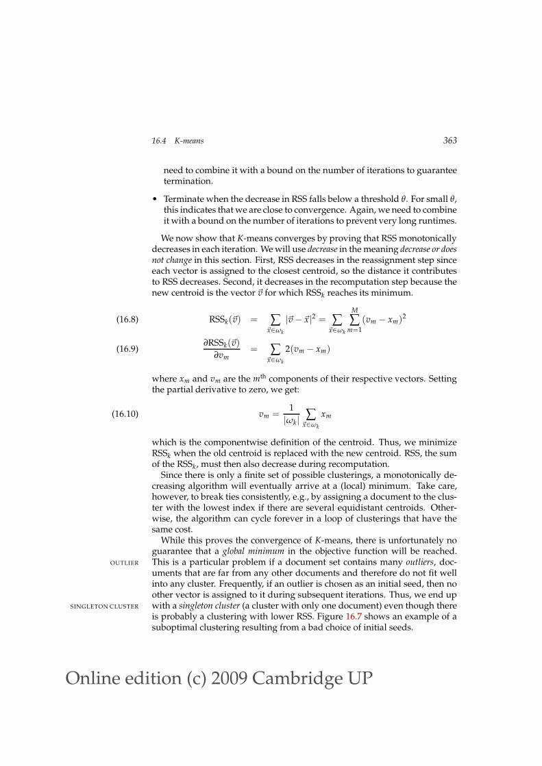
×d1 d2 d3

d4 d5 d6

Figure 16.7 The outcome of clustering in K-means depends on the initial seeds.For seeds d2 and d5, K-means converges to d1, d2, d3, d4, d5, d6, a suboptimalclustering. For seeds d2 and d3, it converges to d1, d2, d4, d5, d3, d6, the globaloptimum for K = 2.

Another type of suboptimal clustering that frequently occurs is one withempty clusters (Exercise 16.11).

Effective heuristics for seed selection include (i) excluding outliers fromthe seed set; (ii) trying out multiple starting points and choosing the cluster-ing with lowest cost; and (iii) obtaining seeds from another method such ashierarchical clustering. Since deterministic hierarchical clustering methodsare more predictable than K-means, a hierarchical clustering of a small ran-dom sample of size iK (e.g., for i = 5 or i = 10) often provides good seeds(see the description of the Buckshot algorithm, Chapter 17, page 399).

Other initialization methods compute seeds that are not selected from thevectors to be clustered. A robust method that works well for a large varietyof document distributions is to select i (e.g., i = 10) random vectors for eachcluster and use their centroid as the seed for this cluster. See Section 16.6 formore sophisticated initializations.

What is the time complexity of K-means? Most of the time is spent on com-puting vector distances. One such operation costs Θ(M). The reassignmentstep computes KN distances, so its overall complexity is Θ(KNM). In therecomputation step, each vector gets added to a centroid once, so the com-plexity of this step is Θ(NM). For a fixed number of iterations I, the overallcomplexity is therefore Θ(IKNM). Thus, K-means is linear in all relevantfactors: iterations, number of clusters, number of vectors and dimensionalityof the space. This means that K-means is more efficient than the hierarchicalalgorithms in Chapter 17. We had to fix the number of iterations I, which canbe tricky in practice. But in most cases, K-means quickly reaches either com-plete convergence or a clustering that is close to convergence. In the lattercase, a few documents would switch membership if further iterations werecomputed, but this has a small effect on the overall quality of the clustering.


16.4 K-means 365

There is one subtlety in the preceding argument. Even a linear algorithmcan be quite slow if one of the arguments of Θ(. . .) is large, and M usually islarge. High dimensionality is not a problem for computing the distance be-tween two documents. Their vectors are sparse, so that only a small fractionof the theoretically possible M componentwise differences need to be com-puted. Centroids, however, are dense since they pool all terms that occur inany of the documents of their clusters. As a result, distance computations aretime consuming in a naive implementation of K-means. However, there aresimple and effective heuristics for making centroid-document similarities asfast to compute as document-document similarities. Truncating centroids tothe most significant k terms (e.g., k = 1000) hardly decreases cluster qualitywhile achieving a significant speedup of the reassignment step (see refer-ences in Section 16.6).

The same efficiency problem is addressed by K-medoids, a variant of K-K-MEDOIDS

means that computes medoids instead of centroids as cluster centers. Wedefine the medoid of a cluster as the document vector that is closest to theMEDOID

centroid. Since medoids are sparse document vectors, distance computationsare fast.

16.4.1 Cluster cardinality in K-means

We stated in Section 16.2 that the number of clusters K is an input to most flatclustering algorithms. What do we do if we cannot come up with a plausibleguess for K?

A naive approach would be to select the optimal value of K according tothe objective function, namely the value of K that minimizes RSS. DefiningRSSmin(K) as the minimal RSS of all clusterings with K clusters, we observethat RSSmin(K) is a monotonically decreasing function in K (Exercise 16.13),which reaches its minimum 0 for K = N where N is the number of doc-uments. We would end up with each document being in its own cluster.Clearly, this is not an optimal clustering.

A heuristic method that gets around this problem is to estimate RSSmin(K)as follows. We first perform i (e.g., i = 10) clusterings with K clusters (eachwith a different initialization) and compute the RSS of each. Then we take the

minimum of the i RSS values. We denote this minimum by RSSmin(K). Now

we can inspect the values RSSmin(K) as K increases and find the “knee” in the

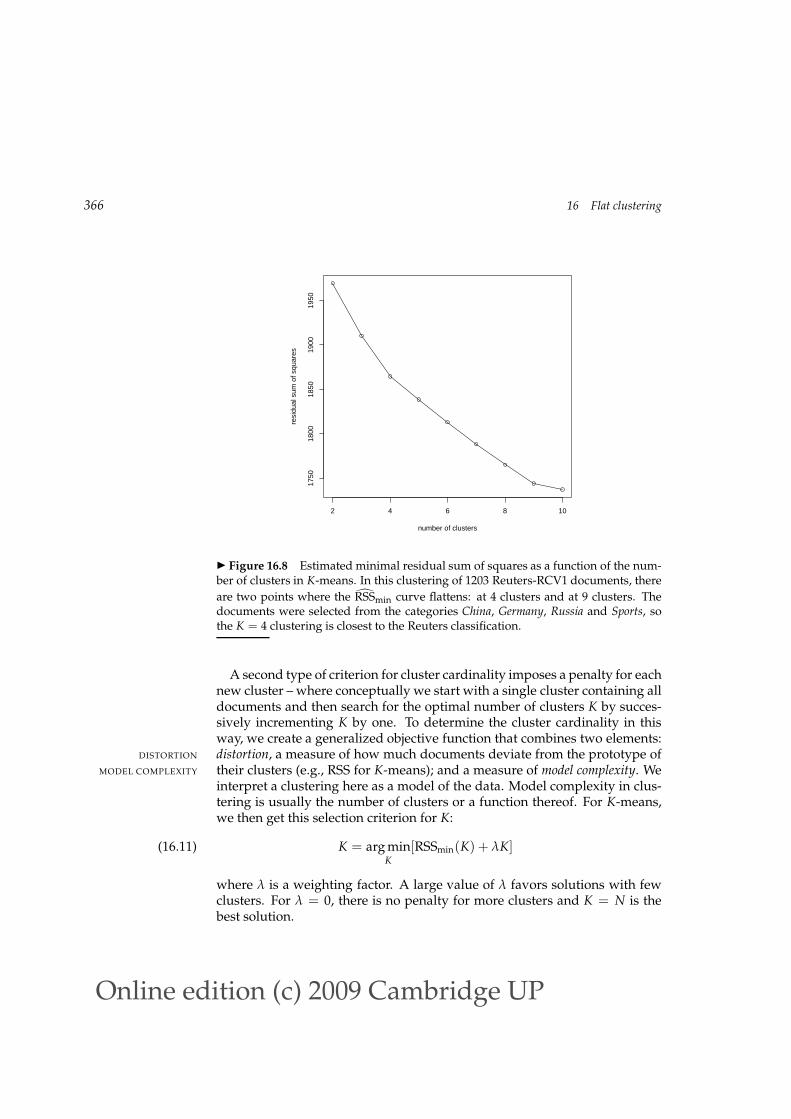
curve – the point where successive decreases in RSSmin become noticeablysmaller. There are two such points in Figure 16.8, one at K = 4, where thegradient flattens slightly, and a clearer flattening at K = 9. This is typical:there is seldom a single best number of clusters. We still need to employ anexternal constraint to choose from a number of possible values of K (4 and 9in this case).



2 4 6 8 10

1750

1800

1850

1900

1950

number of clusters

resi

dual

sum

of s

quar

es

Figure 16.8 Estimated minimal residual sum of squares as a function of the num-ber of clusters in K-means. In this clustering of 1203 Reuters-RCV1 documents, there

are two points where the RSSmin curve flattens: at 4 clusters and at 9 clusters. Thedocuments were selected from the categories China, Germany, Russia and Sports, sothe K = 4 clustering is closest to the Reuters classification.

A second type of criterion for cluster cardinality imposes a penalty for eachnew cluster – where conceptually we start with a single cluster containing alldocuments and then search for the optimal number of clusters K by succes-sively incrementing K by one. To determine the cluster cardinality in thisway, we create a generalized objective function that combines two elements:distortion, a measure of how much documents deviate from the prototype ofDISTORTION

their clusters (e.g., RSS for K-means); and a measure of model complexity. WeMODEL COMPLEXITY

interpret a clustering here as a model of the data. Model complexity in clus-tering is usually the number of clusters or a function thereof. For K-means,we then get this selection criterion for K:

K = arg minK

[RSSmin(K) + λK](16.11)

where λ is a weighting factor. A large value of λ favors solutions with fewclusters. For λ = 0, there is no penalty for more clusters and K = N is thebest solution.


16.4 K-means 367

The obvious difficulty with Equation (16.11) is that we need to determineλ. Unless this is easier than determining K directly, then we are back tosquare one. In some cases, we can choose values of λ that have worked wellfor similar data sets in the past. For example, if we periodically cluster newsstories from a newswire, there is likely to be a fixed value of λ that gives usthe right K in each successive clustering. In this application, we would notbe able to determine K based on past experience since K changes.

A theoretical justification for Equation (16.11) is the Akaike Information Cri-AKAIKE INFORMATION

CRITERION terion or AIC, an information-theoretic measure that trades off distortionagainst model complexity. The general form of AIC is:

AIC: K = arg minK

[−2L(K) + 2q(K)](16.12)

where −L(K), the negative maximum log-likelihood of the data for K clus-ters, is a measure of distortion and q(K), the number of parameters of amodel with K clusters, is a measure of model complexity. We will not at-tempt to derive the AIC here, but it is easy to understand intuitively. Thefirst property of a good model of the data is that each data point is modeledwell by the model. This is the goal of low distortion. But models shouldalso be small (i.e., have low model complexity) since a model that merelydescribes the data (and therefore has zero distortion) is worthless. AIC pro-vides a theoretical justification for one particular way of weighting these twofactors, distortion and model complexity, when selecting a model.

For K-means, the AIC can be stated as follows:

AIC: K = arg minK

[RSSmin(K) + 2MK](16.13)

Equation (16.13) is a special case of Equation (16.11) for λ = 2M.To derive Equation (16.13) from Equation (16.12) observe that q(K) = KM

in K-means since each element of the K centroids is a parameter that can bevaried independently; and that L(K) = −(1/2)RSSmin(K) (modulo a con-stant) if we view the model underlying K-means as a Gaussian mixture withhard assignment, uniform cluster priors and identical spherical covariancematrices (see Exercise 16.19).

The derivation of AIC is based on a number of assumptions, e.g., that thedata are independent and identically distributed. These assumptions areonly approximately true for data sets in information retrieval. As a conse-quence, the AIC can rarely be applied without modification in text clustering.In Figure 16.8, the dimensionality of the vector space is M ≈ 50,000. Thus,

2MK > 50,000 dominates the smaller RSS-based term (RSSmin(1) < 5000,not shown in the figure) and the minimum of the expression is reached forK = 1. But as we know, K = 4 (corresponding to the four classes China,



Germany, Russia and Sports) is a better choice than K = 1. In practice, Equa-tion (16.11) is often more useful than Equation (16.13) – with the caveat thatwe need to come up with an estimate for λ.

? Exercise 16.4

Why are documents that do not use the same term for the concept car likely to endup in the same cluster in K-means clustering?

Exercise 16.5

Two of the possible termination conditions for K-means were (1) assignment does notchange, (2) centroids do not change (page 361). Do these two conditions imply eachother?

16.5 Model-based clustering

In this section, we describe a generalization of K-means, the EM algorithm.It can be applied to a larger variety of document representations and distri-butions than K-means.

In K-means, we attempt to find centroids that are good representatives. Wecan view the set of K centroids as a model that generates the data. Generatinga document in this model consists of first picking a centroid at random andthen adding some noise. If the noise is normally distributed, this procedurewill result in clusters of spherical shape. Model-based clustering assumes thatMODEL-BASED

CLUSTERING the data were generated by a model and tries to recover the original modelfrom the data. The model that we recover from the data then defines clustersand an assignment of documents to clusters.

A commonly used criterion for estimating the model parameters is maxi-mum likelihood. In K-means, the quantity exp(−RSS) is proportional to thelikelihood that a particular model (i.e., a set of centroids) generated the data.For K-means, maximum likelihood and minimal RSS are equivalent criteria.We denote the model parameters by Θ. In K-means, Θ = ~µ1, . . . ,~µK.

More generally, the maximum likelihood criterion is to select the parame-ters Θ that maximize the log-likelihood of generating the data D:

Θ = arg maxΘ

L(D|Θ) = arg maxΘ

logN

∏n=1

P(dn|Θ) = arg maxΘ

N

∑n=1

log P(dn|Θ)

L(D|Θ) is the objective function that measures the goodness of the cluster-ing. Given two clusterings with the same number of clusters, we prefer theone with higher L(D|Θ).

This is the same approach we took in Chapter 12 (page 237) for languagemodeling and in Section 13.1 (page 265) for text classification. In text clas-sification, we chose the class that maximizes the likelihood of generating aparticular document. Here, we choose the clustering Θ that maximizes the


16.5 Model-based clustering 369

likelihood of generating a given set of documents. Once we have Θ, we cancompute an assignment probability P(d|ωk; Θ) for each document-clusterpair. This set of assignment probabilities defines a soft clustering.

An example of a soft assignment is that a document about Chinese carsmay have a fractional membership of 0.5 in each of the two clusters Chinaand automobiles, reflecting the fact that both topics are pertinent. A hard clus-tering like K-means cannot model this simultaneous relevance to two topics.

Model-based clustering provides a framework for incorporating our know-ledge about a domain. K-means and the hierarchical algorithms in Chap-ter 17 make fairly rigid assumptions about the data. For example, clustersin K-means are assumed to be spheres. Model-based clustering offers moreflexibility. The clustering model can be adapted to what we know aboutthe underlying distribution of the data, be it Bernoulli (as in the examplein Table 16.3), Gaussian with non-spherical variance (another model that isimportant in document clustering) or a member of a different family.

A commonly used algorithm for model-based clustering is the Expectation-EXPECTATION-MAXIMIZATION

ALGORITHMMaximization algorithm or EM algorithm. EM clustering is an iterative algo-rithm that maximizes L(D|Θ). EM can be applied to many different types ofprobabilistic modeling. We will work with a mixture of multivariate Bernoullidistributions here, the distribution we know from Section 11.3 (page 222) andSection 13.3 (page 263):

P(d|ωk; Θ) =

(∏

tm∈d

qmk

)(∏

tm /∈d

(1− qmk)

)(16.14)

where Θ = Θ1, . . . , ΘK, Θk = (αk, q1k, . . . , qMk), and qmk = P(Um = 1|ωk)are the parameters of the model.3 P(Um = 1|ωk) is the probability that adocument from cluster ωk contains term tm. The probability αk is the prior ofcluster ωk: the probability that a document d is in ωk if we have no informa-tion about d.

The mixture model then is:

P(d|Θ) =K

∑k=1

αk

(∏

tm∈d

qmk

)(∏

tm /∈d

(1− qmk)

)(16.15)

In this model, we generate a document by first picking a cluster k with prob-ability αk and then generating the terms of the document according to theparameters qmk. Recall that the document representation of the multivariateBernoulli is a vector of M Boolean values (and not a real-valued vector).

3. Um is the random variable we defined in Section 13.3 (page 266) for the Bernoulli Naive Bayesmodel. It takes the values 1 (term tm is present in the document) and 0 (term tm is absent in thedocument).



How do we use EM to infer the parameters of the clustering from the data?That is, how do we choose parameters Θ that maximize L(D|Θ)? EM is simi-lar to K-means in that it alternates between an expectation step, correspondingEXPECTATION STEP

to reassignment, and a maximization step, corresponding to recomputation ofMAXIMIZATION STEP

the parameters of the model. The parameters of K-means are the centroids,the parameters of the instance of EM in this section are the αk and qmk.

The maximization step recomputes the conditional parameters qmk and thepriors αk as follows:

Maximization step: qmk =∑

Nn=1 rnk I(tm ∈ dn)

∑Nn=1 rnk

αk =∑

Nn=1 rnk

N(16.16)

where I(tm ∈ dn) = 1 if tm ∈ dn and 0 otherwise and rnk is the soft as-signment of document dn to cluster k as computed in the preceding iteration.(We’ll address the issue of initialization in a moment.) These are the max-imum likelihood estimates for the parameters of the multivariate Bernoullifrom Table 13.3 (page 268) except that documents are assigned fractionally toclusters here. These maximum likelihood estimates maximize the likelihoodof the data given the model.

The expectation step computes the soft assignment of documents to clus-ters given the current parameters qmk and αk:

Expectation step : rnk =αk(∏tm∈dn

qmk)(∏tm /∈dn(1− qmk))

∑Kk=1 αk(∏tm∈dn

qmk)(∏tm /∈dn(1− qmk))

(16.17)

This expectation step applies Equations (16.14) and (16.15) to computing thelikelihood that ωk generated document dn. It is the classification procedurefor the multivariate Bernoulli in Table 13.3. Thus, the expectation step isnothing else but Bernoulli Naive Bayes classification (including normaliza-tion, i.e. dividing by the denominator, to get a probability distribution overclusters).

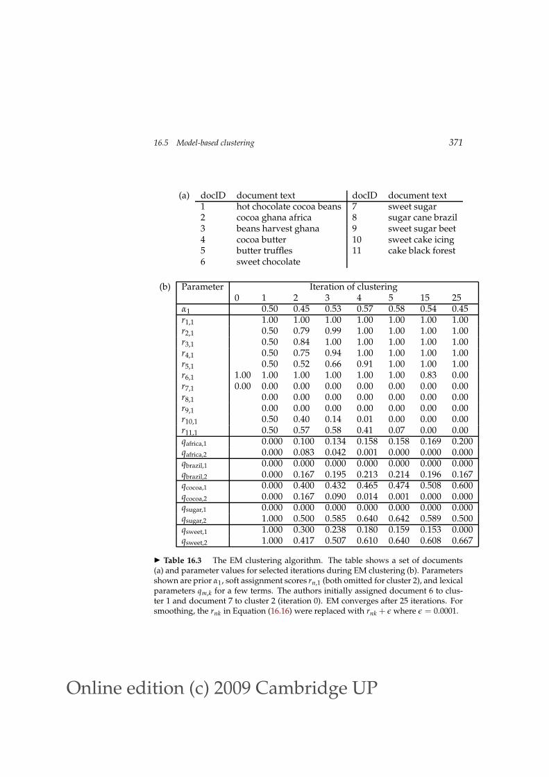
We clustered a set of 11 documents into two clusters using EM in Ta-ble 16.3. After convergence in iteration 25, the first 5 documents are assignedto cluster 1 (ri,1 = 1.00) and the last 6 to cluster 2 (ri,1 = 0.00). Somewhatatypically, the final assignment is a hard assignment here. EM usually con-verges to a soft assignment. In iteration 25, the prior α1 for cluster 1 is5/11 ≈ 0.45 because 5 of the 11 documents are in cluster 1. Some termsare quickly associated with one cluster because the initial assignment can“spread” to them unambiguously. For example, membership in cluster 2spreads from document 7 to document 8 in the first iteration because theyshare sugar (r8,1 = 0 in iteration 1). For parameters of terms occurringin ambiguous contexts, convergence takes longer. Seed documents 6 and 7


16.5 Model-based clustering 371

(a) docID document text docID document text1 hot chocolate cocoa beans 7 sweet sugar2 cocoa ghana africa 8 sugar cane brazil3 beans harvest ghana 9 sweet sugar beet4 cocoa butter 10 sweet cake icing5 butter truffles 11 cake black forest6 sweet chocolate

(b) Parameter Iteration of clustering0 1 2 3 4 5 15 25

α1 0.50 0.45 0.53 0.57 0.58 0.54 0.45r1,1 1.00 1.00 1.00 1.00 1.00 1.00 1.00r2,1 0.50 0.79 0.99 1.00 1.00 1.00 1.00r3,1 0.50 0.84 1.00 1.00 1.00 1.00 1.00r4,1 0.50 0.75 0.94 1.00 1.00 1.00 1.00r5,1 0.50 0.52 0.66 0.91 1.00 1.00 1.00r6,1 1.00 1.00 1.00 1.00 1.00 1.00 0.83 0.00r7,1 0.00 0.00 0.00 0.00 0.00 0.00 0.00 0.00r8,1 0.00 0.00 0.00 0.00 0.00 0.00 0.00r9,1 0.00 0.00 0.00 0.00 0.00 0.00 0.00r10,1 0.50 0.40 0.14 0.01 0.00 0.00 0.00r11,1 0.50 0.57 0.58 0.41 0.07 0.00 0.00qafrica,1 0.000 0.100 0.134 0.158 0.158 0.169 0.200qafrica,2 0.000 0.083 0.042 0.001 0.000 0.000 0.000qbrazil,1 0.000 0.000 0.000 0.000 0.000 0.000 0.000qbrazil,2 0.000 0.167 0.195 0.213 0.214 0.196 0.167qcocoa,1 0.000 0.400 0.432 0.465 0.474 0.508 0.600qcocoa,2 0.000 0.167 0.090 0.014 0.001 0.000 0.000qsugar,1 0.000 0.000 0.000 0.000 0.000 0.000 0.000qsugar,2 1.000 0.500 0.585 0.640 0.642 0.589 0.500qsweet,1 1.000 0.300 0.238 0.180 0.159 0.153 0.000qsweet,2 1.000 0.417 0.507 0.610 0.640 0.608 0.667

Table 16.3 The EM clustering algorithm. The table shows a set of documents(a) and parameter values for selected iterations during EM clustering (b). Parametersshown are prior α1, soft assignment scores rn,1 (both omitted for cluster 2), and lexicalparameters qm,k for a few terms. The authors initially assigned document 6 to clus-ter 1 and document 7 to cluster 2 (iteration 0). EM converges after 25 iterations. Forsmoothing, the rnk in Equation (16.16) were replaced with rnk + ǫ where ǫ = 0.0001.



both contain sweet. As a result, it takes 25 iterations for the term to be unam-biguously associated with cluster 2. (qsweet,1 = 0 in iteration 25.)

Finding good seeds is even more critical for EM than for K-means. EM isprone to get stuck in local optima if the seeds are not chosen well. This is ageneral problem that also occurs in other applications of EM.4 Therefore, aswith K-means, the initial assignment of documents to clusters is often com-puted by a different algorithm. For example, a hard K-means clustering mayprovide the initial assignment, which EM can then “soften up.”

? Exercise 16.6

We saw above that the time complexity of K-means is Θ(IKNM). What is the timecomplexity of EM?

16.6 References and further reading

Berkhin (2006b) gives a general up-to-date survey of clustering methods withspecial attention to scalability. The classic reference for clustering in pat-tern recognition, covering both K-means and EM, is (Duda et al. 2000). Ras-mussen (1992) introduces clustering from an information retrieval perspec-tive. Anderberg (1973) provides a general introduction to clustering for ap-plications. In addition to Euclidean distance and cosine similarity, Kullback-Leibler divergence is often used in clustering as a measure of how (dis)similardocuments and clusters are (Xu and Croft 1999, Muresan and Harper 2004,Kurland and Lee 2004).

The cluster hypothesis is due to Jardine and van Rijsbergen (1971) whostate it as follows: Associations between documents convey information about therelevance of documents to requests. Salton (1971a; 1975), Croft (1978), Voorhees(1985a), Can and Ozkarahan (1990), Cacheda et al. (2003), Can et al. (2004),Singitham et al. (2004) and Altingövde et al. (2008) investigate the efficiencyand effectiveness of cluster-based retrieval. While some of these studiesshow improvements in effectiveness, efficiency or both, there is no consensusthat cluster-based retrieval works well consistently across scenarios. Cluster-based language modeling was pioneered by Liu and Croft (2004).

There is good evidence that clustering of search results improves user ex-perience and search result quality (Hearst and Pedersen 1996, Zamir and Et-zioni 1999, Tombros et al. 2002, Käki 2005, Toda and Kataoka 2005), althoughnot as much as search result structuring based on carefully edited categoryhierarchies (Hearst 2006). The Scatter-Gather interface for browsing collec-tions was presented by Cutting et al. (1992). A theoretical framework for an-

4. For example, this problem is common when EM is used to estimate parameters of hiddenMarkov models, probabilistic grammars, and machine translation models in natural languageprocessing (Manning and Schütze 1999).


16.6 References and further reading 373

alyzing the properties of Scatter/Gather and other information seeking userinterfaces is presented by Pirolli (2007). Schütze and Silverstein (1997) eval-uate LSI (Chapter 18) and truncated representations of centroids for efficientK-means clustering.

The Columbia NewsBlaster system (McKeown et al. 2002), a forerunner tothe now much more famous and refined Google News (http://news.google.com),used hierarchical clustering (Chapter 17) to give two levels of news topicgranularity. See Hatzivassiloglou et al. (2000) for details, and Chen and Lin(2000) and Radev et al. (2001) for related systems. Other applications ofclustering in information retrieval are duplicate detection (Yang and Callan(2006), Section 19.6, page 438), novelty detection (see references in Section 17.9,page 399) and metadata discovery on the semantic web (Alonso et al. 2006).

The discussion of external evaluation measures is partially based on Strehl(2002). Dom (2002) proposes a measure Q0 that is better motivated theoret-ically than NMI. Q0 is the number of bits needed to transmit class member-ships assuming cluster memberships are known. The Rand index is due toRand (1971). Hubert and Arabie (1985) propose an adjusted Rand index thatADJUSTED RAND INDEX

ranges between −1 and 1 and is 0 if there is only chance agreement betweenclusters and classes (similar to κ in Chapter 8, page 165). Basu et al. (2004) ar-gue that the three evaluation measures NMI, Rand index and F measure givevery similar results. Stein et al. (2003) propose expected edge density as an in-ternal measure and give evidence that it is a good predictor of the quality of aclustering. Kleinberg (2002) and Meila (2005) present axiomatic frameworksfor comparing clusterings.

Authors that are often credited with the invention of the K-means algo-rithm include Lloyd (1982) (first distributed in 1957), Ball (1965), MacQueen(1967), and Hartigan and Wong (1979). Arthur and Vassilvitskii (2006) in-vestigate the worst-case complexity of K-means. Bradley and Fayyad (1998),Pelleg and Moore (1999) and Davidson and Satyanarayana (2003) investi-gate the convergence properties of K-means empirically and how it dependson initial seed selection. Dhillon and Modha (2001) compare K-means clus-ters with SVD-based clusters (Chapter 18). The K-medoid algorithm waspresented by Kaufman and Rousseeuw (1990). The EM algorithm was orig-inally introduced by Dempster et al. (1977). An in-depth treatment of EM is(McLachlan and Krishnan 1996). See Section 18.5 (page 417) for publicationson latent analysis, which can also be viewed as soft clustering.

AIC is due to Akaike (1974) (see also Burnham and Anderson (2002)). Analternative to AIC is BIC, which can be motivated as a Bayesian model se-lection procedure (Schwarz 1978). Fraley and Raftery (1998) show how tochoose an optimal number of clusters based on BIC. An application of BIC toK-means is (Pelleg and Moore 2000). Hamerly and Elkan (2003) propose analternative to BIC that performs better in their experiments. Another influ-ential Bayesian approach for determining the number of clusters (simultane-



ously with cluster assignment) is described by Cheeseman and Stutz (1996).Two methods for determining cardinality without external criteria are pre-sented by Tibshirani et al. (2001).

We only have space here for classical completely unsupervised clustering.An important current topic of research is how to use prior knowledge toguide clustering (e.g., Ji and Xu (2006)) and how to incorporate interactivefeedback during clustering (e.g., Huang and Mitchell (2006)). Fayyad et al.(1998) propose an initialization for EM clustering. For algorithms that cancluster very large data sets in one scan through the data see Bradley et al.(1998).

The applications in Table 16.1 all cluster documents. Other information re-trieval applications cluster words (e.g., Crouch 1988), contexts of words (e.g.,Schütze and Pedersen 1995) or words and documents simultaneously (e.g.,Tishby and Slonim 2000, Dhillon 2001, Zha et al. 2001). Simultaneous clus-tering of words and documents is an example of co-clustering or biclustering.CO-CLUSTERING

16.7 Exercises

? Exercise 16.7

Let Ω be a clustering that exactly reproduces a class structure C and Ω′ a clusteringthat further subdivides some clusters in Ω. Show that I(Ω; C) = I(Ω′; C).

Exercise 16.8

Show that I(Ω; C) ≤ [H(Ω) + H(C)]/2.

Exercise 16.9

Mutual information is symmetric in the sense that its value does not change if theroles of clusters and classes are switched: I(Ω; C) = I(C; Ω). Which of the otherthree evaluation measures are symmetric in this sense?

Exercise 16.10

Compute RSS for the two clusterings in Figure 16.7.

Exercise 16.11

(i) Give an example of a set of points and three initial centroids (which need not bemembers of the set of points) for which 3-means converges to a clustering with anempty cluster. (ii) Can a clustering with an empty cluster be the global optimum withrespect to RSS?

Exercise 16.12

Download Reuters-21578. Discard documents that do not occur in one of the 10classes acquisitions, corn, crude, earn, grain, interest, money-fx, ship, trade, and wheat.Discard documents that occur in two of these 10 classes. (i) Compute a K-means clus-tering of this subset into 10 clusters. There are a number of software packages thatimplement K-means, such as WEKA (Witten and Frank 2005) and R (R DevelopmentCore Team 2005). (ii) Compute purity, normalized mutual information, F1 and RI for


16.7 Exercises 375

the clustering with respect to the 10 classes. (iii) Compile a confusion matrix (Ta-ble 14.5, page 308) for the 10 classes and 10 clusters. Identify classes that give rise tofalse positives and false negatives.

Exercise 16.13

Prove that RSSmin(K) is monotonically decreasing in K.

Exercise 16.14

There is a soft version of K-means that computes the fractional membership of a doc-ument in a cluster as a monotonically decreasing function of the distance ∆ from its

centroid, e.g., as e−∆. Modify reassignment and recomputation steps of hard K-meansfor this soft version.

Exercise 16.15

In the last iteration in Table 16.3, document 6 is in cluster 2 even though it was theinitial seed for cluster 1. Why does the document change membership?

Exercise 16.16

The values of the parameters qmk in iteration 25 in Table 16.3 are rounded. What arethe exact values that EM will converge to?

Exercise 16.17

Perform a K-means clustering for the documents in Table 16.3. After how manyiterations does K-means converge? Compare the result with the EM clustering inTable 16.3 and discuss the differences.

Exercise 16.18 [⋆ ⋆ ⋆]

Modify the expectation and maximization steps of EM for a Gaussian mixture. Themaximization step computes the maximum likelihood parameter estimates αk, ~µk,and Σk for each of the clusters. The expectation step computes for each vector a softassignment to clusters (Gaussians) based on their current parameters. Write downthe equations for Gaussian mixtures corresponding to Equations (16.16) and (16.17).

Exercise 16.19 [⋆ ⋆ ⋆]

Show that K-means can be viewed as the limiting case of EM for Gaussian mixturesif variance is very small and all covariances are 0.

Exercise 16.20 [⋆ ⋆ ⋆]

The within-point scatter of a clustering is defined as ∑k12 ∑~xi∈ωk

∑~xj∈ωk|~xi−~xj|

2. ShowWITHIN-POINT

SCATTER that minimizing RSS and minimizing within-point scatter are equivalent.

Exercise 16.21 [⋆ ⋆ ⋆]

Derive an AIC criterion for the multivariate Bernoulli mixture model from Equa-tion (16.12).