Introduction to Information Retrieval - smbidoki.irsmbidoki.ir/courses/254_IR_932_lecture4_tfidf-2.pdf · Introduction to Information Retrieval tf-idf weighting The tf-idf weight

Introduction to Information Retrieval

Introduction to

Information Retrieval

CS276: Information Retrieval and Web Search

Christopher Manning and Prabhakar Raghavan

Lecture 6: Scoring, Term Weighting and the

Vector Space Model


This lecture; IIR Sections 6.2-6.4.3

Ranked retrieval

Scoring documents

Term frequency

Collection statistics

Weighting schemes

Vector space scoring


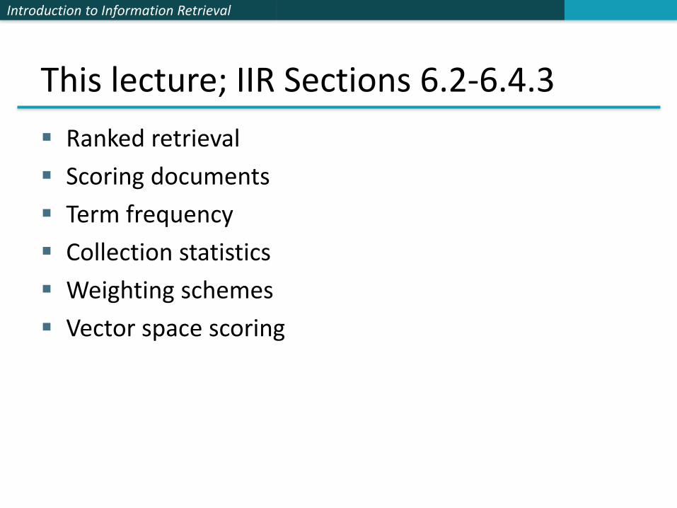
Binary term-document incidence matrix

Antony and Cleopatra Julius Caesar The Tempest Hamlet Othello Macbeth

Antony 1 1 0 0 0 1

Brutus 1 1 0 1 0 0

Caesar 1 1 0 1 1 1

Calpurnia 0 1 0 0 0 0

Cleopatra 1 0 0 0 0 0

mercy 1 0 1 1 1 1

worser 1 0 1 1 1 0

Each document is represented by a binary vector ∈ {0,1}|V|

Sec. 6.2


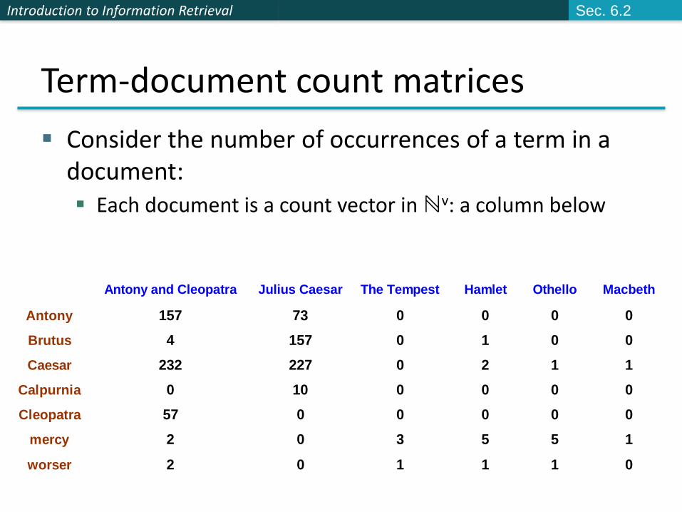
Term-document count matrices

Consider the number of occurrences of a term in a document: Each document is a count vector in ℕv: a column below


Antony 157 73 0 0 0 0

Brutus 4 157 0 1 0 0

Caesar 232 227 0 2 1 1

Calpurnia 0 10 0 0 0 0

Cleopatra 57 0 0 0 0 0

mercy 2 0 3 5 5 1

worser 2 0 1 1 1 0

Sec. 6.2


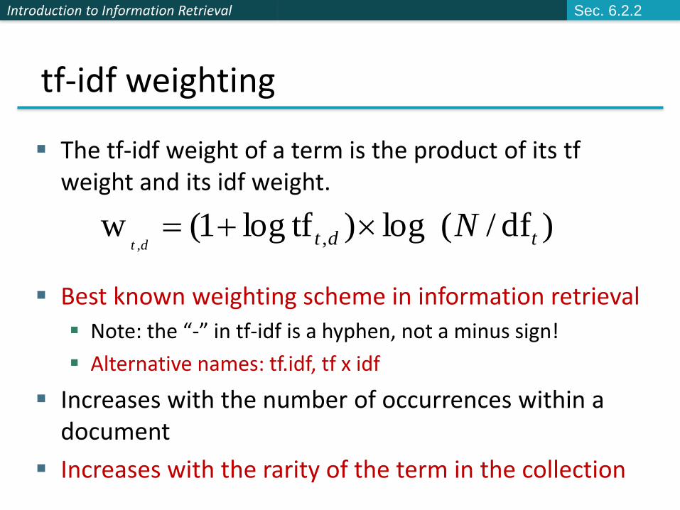
tf-idf weighting

The tf-idf weight of a term is the product of its tfweight and its idf weight.

Best known weighting scheme in information retrieval

Note: the “-” in tf-idf is a hyphen, not a minus sign!

Alternative names: tf.idf, tf x idf

Increases with the number of occurrences within a document

Increases with the rarity of the term in the collection

)df/(log)tflog1(w ,, tdt Ndt

Sec. 6.2.2


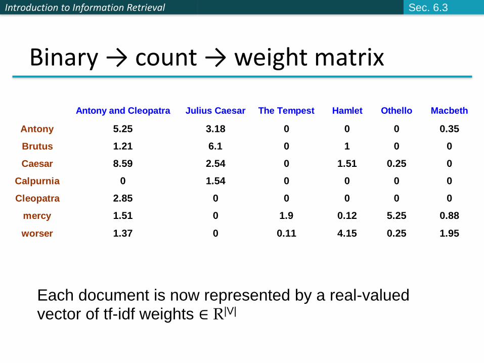
Binary → count → weight matrix


Antony 5.25 3.18 0 0 0 0.35

Brutus 1.21 6.1 0 1 0 0

Caesar 8.59 2.54 0 1.51 0.25 0

Calpurnia 0 1.54 0 0 0 0

Cleopatra 2.85 0 0 0 0 0

mercy 1.51 0 1.9 0.12 5.25 0.88

worser 1.37 0 0.11 4.15 0.25 1.95

Each document is now represented by a real-valued vector of tf-idf weights ∈ R|V|

Sec. 6.3


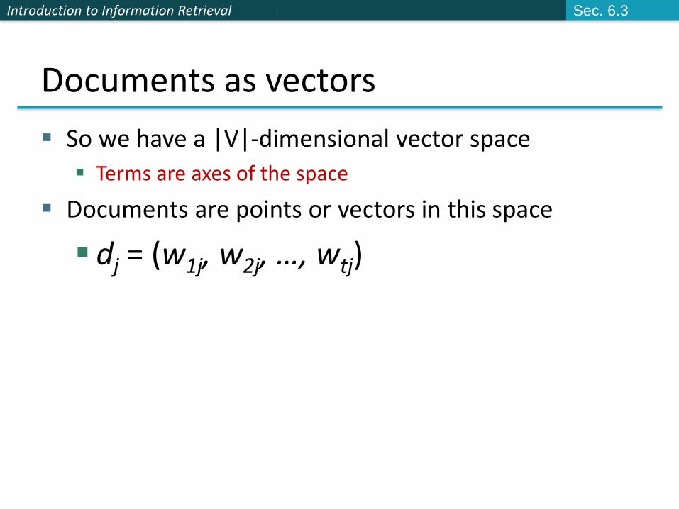
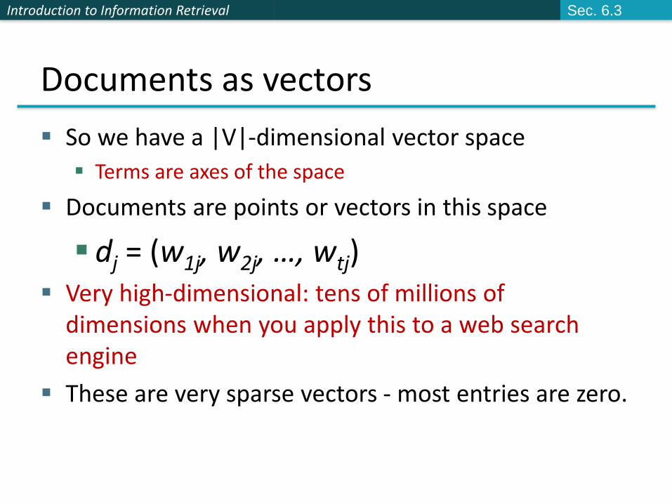
Documents as vectors

So we have a |V|-dimensional vector space

Terms are axes of the space

Documents are points or vectors in this space

dj = (w1j, w2j, …, wtj)

Sec. 6.3


8

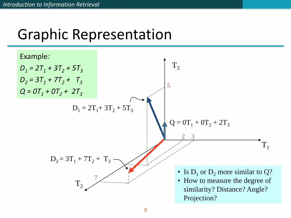
Graphic RepresentationExample:

D1 = 2T1 + 3T2 + 5T3

D2 = 3T1 + 7T2 + T3

Q = 0T1 + 0T2 + 2T3

T3

T1

T2

D1 = 2T1+ 3T2 + 5T3

D2 = 3T1 + 7T2 + T3

Q = 0T1 + 0T2 + 2T3

7

32

5

• Is D1 or D2 more similar to Q?

• How to measure the degree of

similarity? Distance? Angle?

Projection?


Documents as vectors

So we have a |V|-dimensional vector space

Terms are axes of the space

Documents are points or vectors in this space

dj = (w1j, w2j, …, wtj) Very high-dimensional: tens of millions of

dimensions when you apply this to a web search engine

These are very sparse vectors - most entries are zero.

Sec. 6.3


10

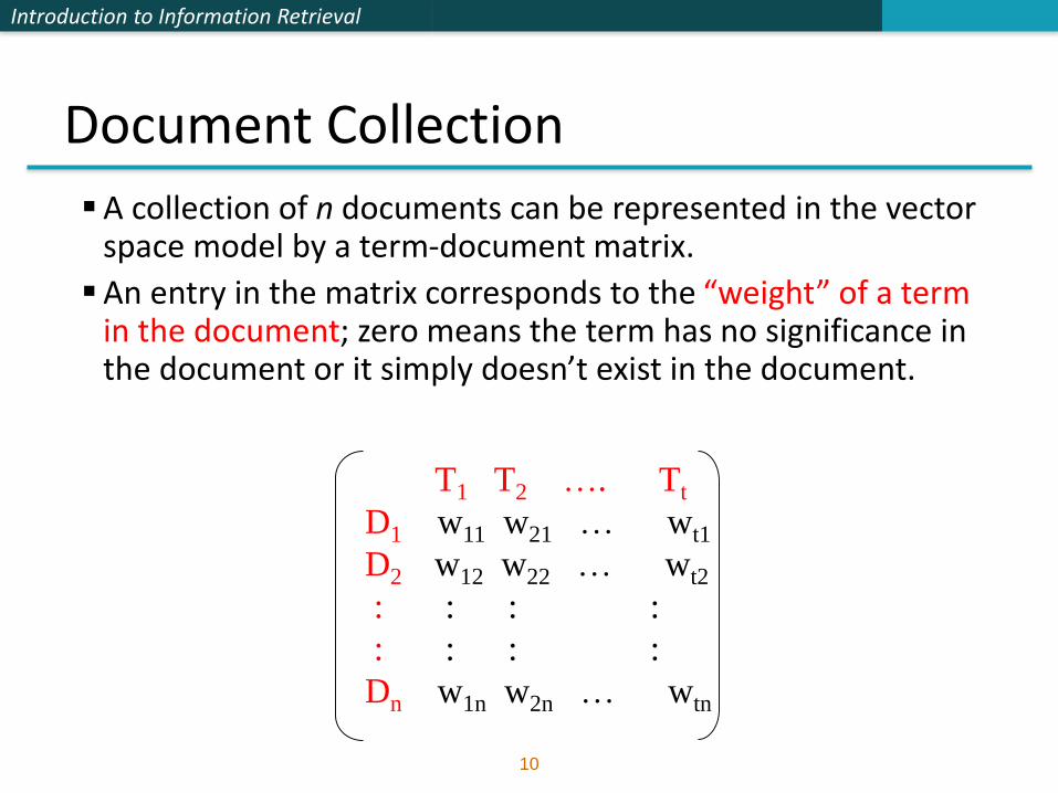
Document Collection

A collection of n documents can be represented in the vector space model by a term-document matrix.

An entry in the matrix corresponds to the “weight” of a term in the document; zero means the term has no significance in the document or it simply doesn’t exist in the document.

T1 T2 …. Tt

D1 w11 w21 … wt1

D2 w12 w22 … wt2

: : : :

: : : :

Dn w1n w2n … wtn


Queries as vectors

Key idea 1: Do the same for queries: represent them as vectors in the space

Key idea 2: Rank documents according to their proximity to the query in this space

proximity = similarity of vectors

proximity ≈ inverse of distance

rank more relevant documents higher than less relevant documents

It is possible to enforce a certain threshold so that the size of the retrieved set can be controlled.

Sec. 6.3


Formalizing vector space proximity

First cut: distance between two points

( = distance between the end points of the two vectors)

Euclidean distance?

Euclidean distance is a bad idea . . .

. . . because Euclidean distance is large for vectors of different lengths.

Sec. 6.3


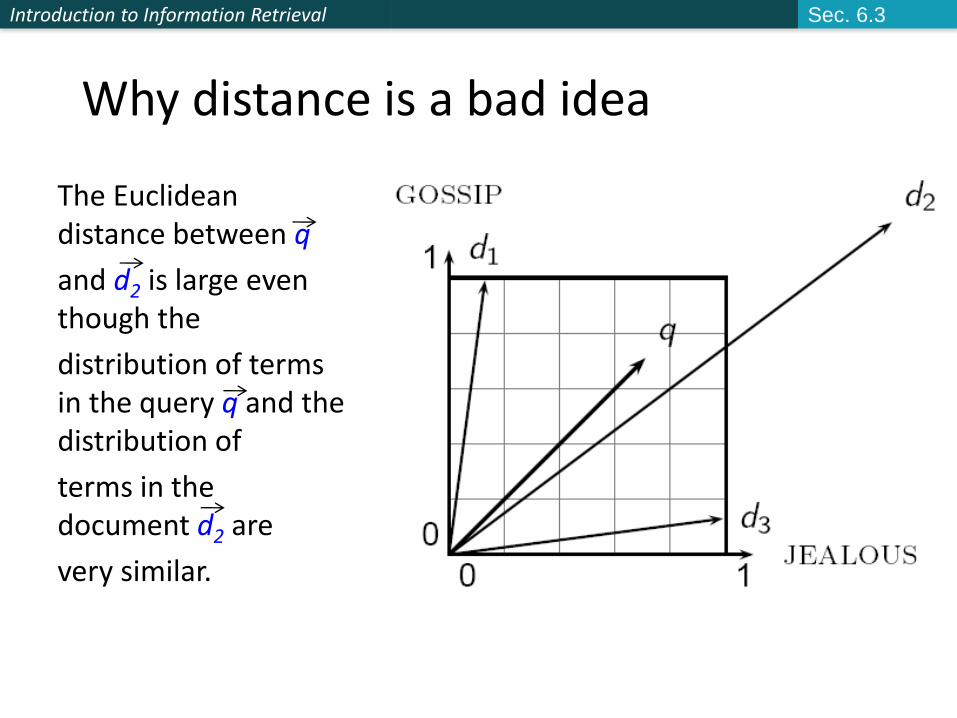
Why distance is a bad idea

The Euclidean distance between q

and d2 is large even though the

distribution of terms in the query q and the distribution of

terms in the document d2 are

very similar.

Sec. 6.3


Use angle instead of distance

Thought experiment: take a document d and append it to itself. Call this document d′.

“Semantically” d and d′ have the same content

The Euclidean distance between the two documents can be quite large

The angle between the two documents is 0, corresponding to maximal similarity.

Key idea: Rank documents according to angle with query.

Sec. 6.3


15

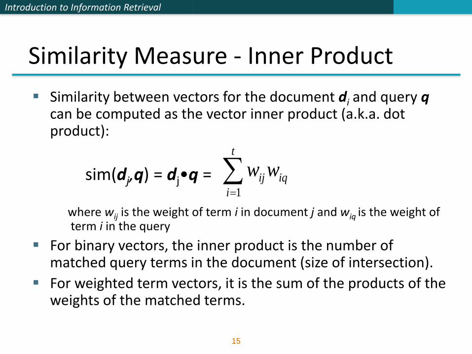
Similarity Measure - Inner Product

Similarity between vectors for the document di and query qcan be computed as the vector inner product (a.k.a. dot product):

sim(dj,q) = dj•q =

where wij is the weight of term i in document j and wiq is the weight of term i in the query

For binary vectors, the inner product is the number of matched query terms in the document (size of intersection).

For weighted term vectors, it is the sum of the products of the weights of the matched terms.

iq

t

i

ijww1


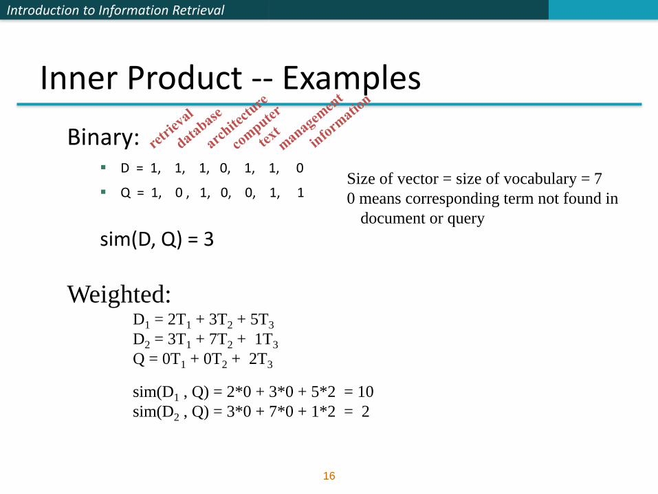
16

Inner Product -- Examples

Binary: D = 1, 1, 1, 0, 1, 1, 0

Q = 1, 0 , 1, 0, 0, 1, 1

sim(D, Q) = 3

Size of vector = size of vocabulary = 7

0 means corresponding term not found in

document or query

Weighted:D1 = 2T1 + 3T2 + 5T3

D2 = 3T1 + 7T2 + 1T3

Q = 0T1 + 0T2 + 2T3

sim(D1 , Q) = 2*0 + 3*0 + 5*2 = 10

sim(D2 , Q) = 3*0 + 7*0 + 1*2 = 2


17

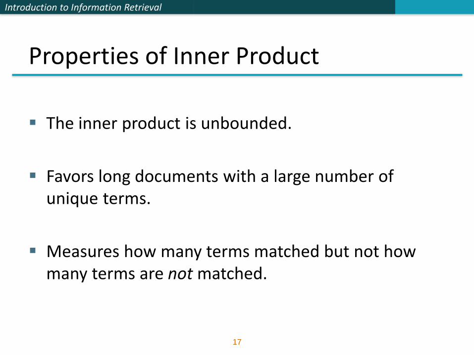
Properties of Inner Product

The inner product is unbounded.

Favors long documents with a large number of unique terms.

Measures how many terms matched but not how many terms are not matched.


From angles to cosines

The following two notions are equivalent.

Rank documents in increasing order of the angle between query and document

Rank documents in decreasing order of cosine(angle between query,document)

Cosine is a monotonically decreasing function for the interval [0o, 180o]

Sec. 6.3


From angles to cosines

But how – and why – should we be computing cosines?

Sec. 6.3


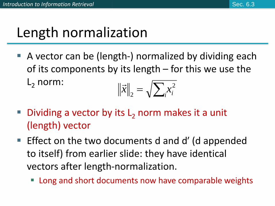
Length normalization

A vector can be (length-) normalized by dividing each of its components by its length – for this we use the L2 norm:

Dividing a vector by its L2 norm makes it a unit (length) vector

Effect on the two documents d and d′ (d appended to itself) from earlier slide: they have identical vectors after length-normalization.

Long and short documents now have comparable weights

i ixx 2

2

Sec. 6.3


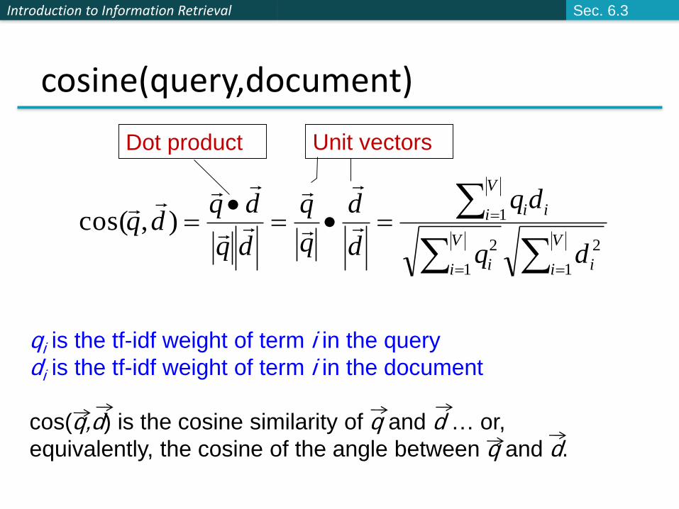
cosine(query,document)

V

i i

V

i i

V

i ii

dq

dq

d

d

q

q

dq

dqdq

1

2

1

2

1),cos(

Dot product Unit vectors

qi is the tf-idf weight of term i in the query

di is the tf-idf weight of term i in the document

cos(q,d) is the cosine similarity of q and d … or,

equivalently, the cosine of the angle between q and d.

Sec. 6.3


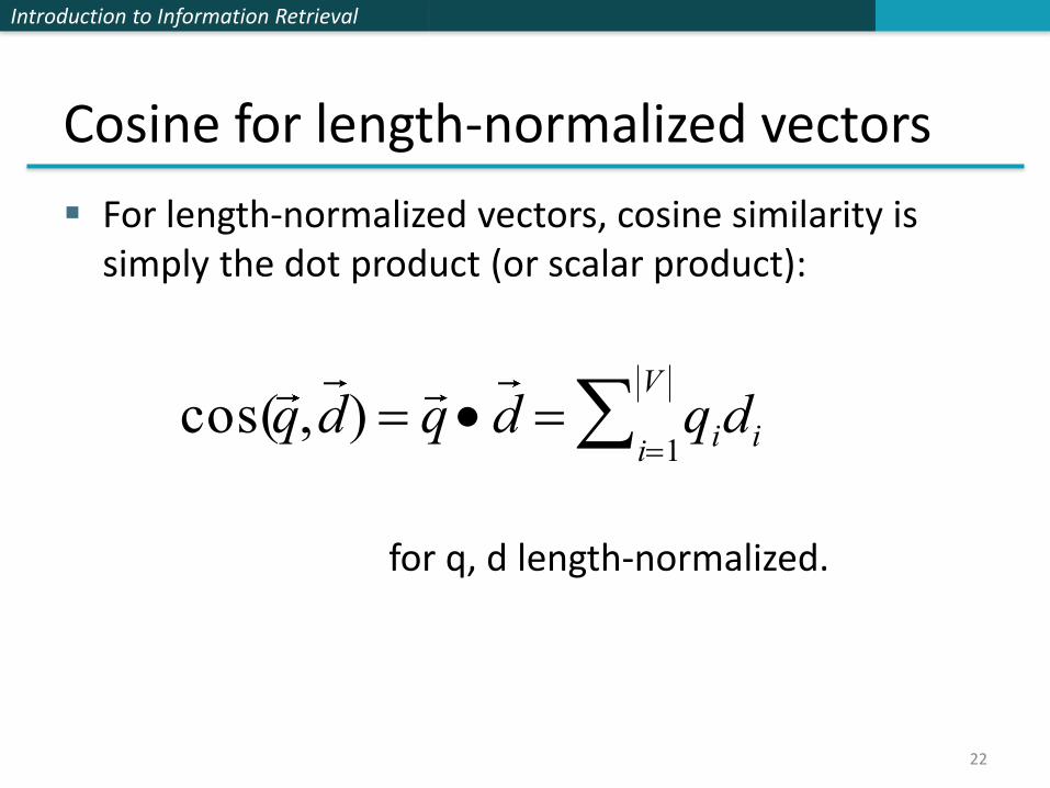
Cosine for length-normalized vectors

For length-normalized vectors, cosine similarity is simply the dot product (or scalar product):

for q, d length-normalized.

22

cos(q ,d ) q d qidii1

V


Cosine similarity illustrated

23


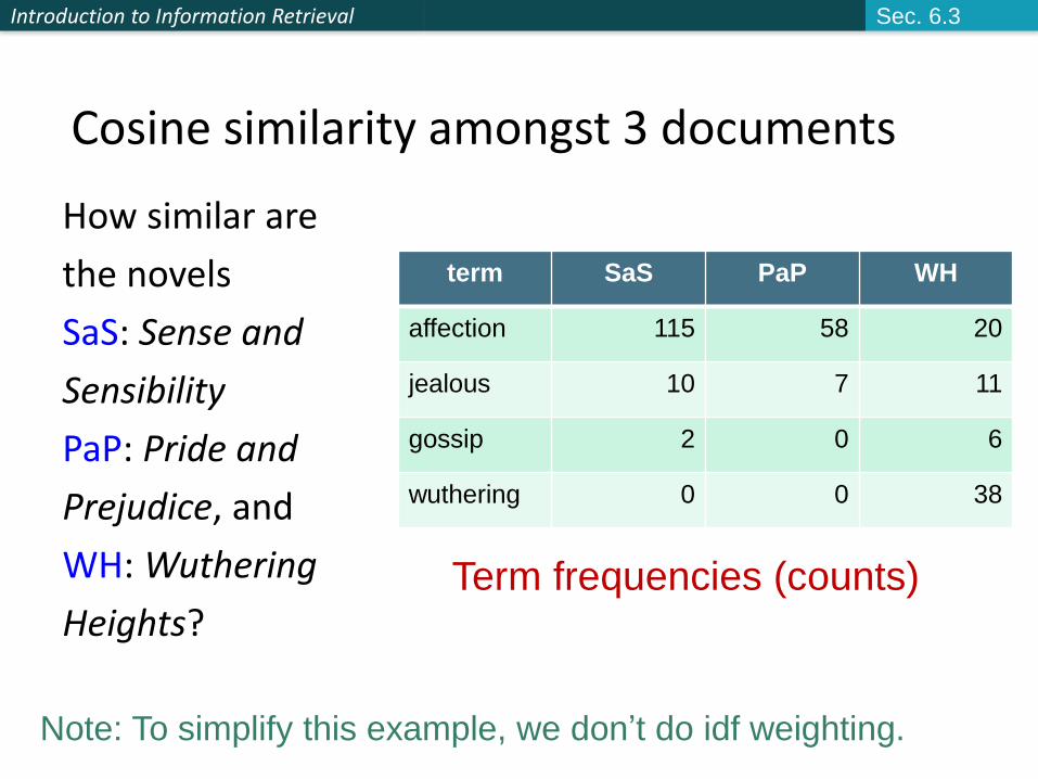
Cosine similarity amongst 3 documents

term SaS PaP WH

affection 115 58 20

jealous 10 7 11

gossip 2 0 6

wuthering 0 0 38

How similar are

the novels

SaS: Sense and

Sensibility

PaP: Pride and

Prejudice, and

WH: Wuthering

Heights?Term frequencies (counts)

Sec. 6.3

Note: To simplify this example, we don’t do idf weighting.


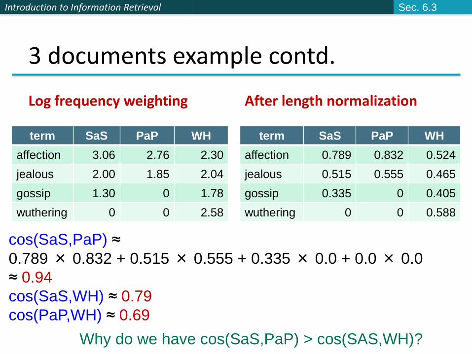
3 documents example contd.

Log frequency weighting

term SaS PaP WH

affection 3.06 2.76 2.30

jealous 2.00 1.85 2.04

gossip 1.30 0 1.78

wuthering 0 0 2.58

After length normalization

term SaS PaP WH

affection 0.789 0.832 0.524

jealous 0.515 0.555 0.465

gossip 0.335 0 0.405

wuthering 0 0 0.588

cos(SaS,PaP) ≈

0.789 × 0.832 + 0.515 × 0.555 + 0.335 × 0.0 + 0.0 × 0.0

≈ 0.94

cos(SaS,WH) ≈ 0.79

cos(PaP,WH) ≈ 0.69

Why do we have cos(SaS,PaP) > cos(SAS,WH)?

Sec. 6.3


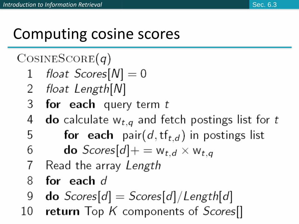
Computing cosine scores

Sec. 6.3


Summary – vector space ranking

Represent the query as a weighted tf-idf vector

Represent each document as a weighted tf-idf vector

Compute the cosine similarity score for the query vector and each document vector

Rank documents with respect to the query by score

Return the top K (e.g., K = 10) to the user


28

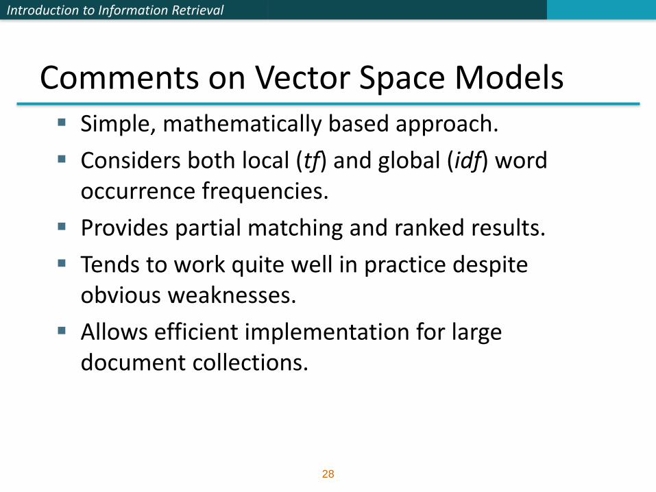
Comments on Vector Space Models Simple, mathematically based approach.

Considers both local (tf) and global (idf) word occurrence frequencies.

Provides partial matching and ranked results.

Tends to work quite well in practice despite obvious weaknesses.

Allows efficient implementation for large document collections.


29

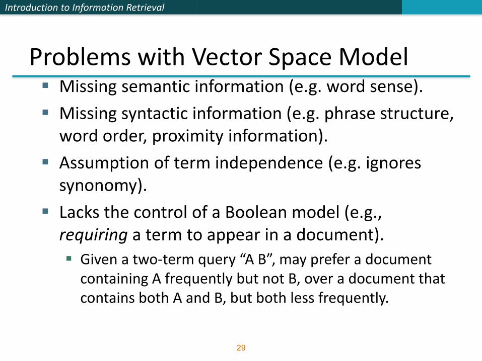
Problems with Vector Space Model Missing semantic information (e.g. word sense).

Missing syntactic information (e.g. phrase structure, word order, proximity information).

Assumption of term independence (e.g. ignores synonomy).

Lacks the control of a Boolean model (e.g., requiring a term to appear in a document).

Given a two-term query “A B”, may prefer a document containing A frequently but not B, over a document that contains both A and B, but both less frequently.


Resources for today’s lecture

IIR 6.2 – 6.4.3

http://www.miislita.com/information-retrieval-tutorial/cosine-similarity-tutorial.html

Term weighting and cosine similarity tutorial for SEO folk!

Ch. 6

http://www.miislita.com/information-retrieval-tutorial/cosine-similarity-tutorial.html