Introduction to Information Retrievalhttp://informationretrieval.org

IIR 13: Text Classification & Naive Bayes

Hinrich Schutze

Center for Information and Language Processing, University of Munich

2014-05-15

1 / 58

Overview

1 Recap

2 Text classification

3 Naive Bayes

4 NB theory

5 Evaluation of TC

2 / 58

Outline

1 Recap

2 Text classification

3 Naive Bayes

4 NB theory

5 Evaluation of TC

3 / 58

Relevance feedback: Basic idea

The user issues a (short, simple) query.

The search engine returns a set of documents.

User marks some docs as relevant, some as nonrelevant.

Search engine computes a new representation of theinformation need – should be better than the initial query.

Search engine runs new query and returns new results.

New results have (hopefully) better recall.

4 / 58

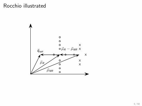
Rocchio illustrated

x

x

x

x

xx

~µR

~µNR

~µR − ~µNR~qopt

5 / 58

Types of query expansion

Manual thesaurus (maintained by editors, e.g., PubMed)

Automatically derived thesaurus (e.g., based on co-occurrencestatistics)

Query-equivalence based on query log mining (common on theweb as in the “palm” example)

6 / 58

Query expansion at search engines

Main source of query expansion at search engines: query logs

Example 1: After issuing the query [herbs], users frequentlysearch for [herbal remedies].

→ “herbal remedies” is potential expansion of “herb”.

Example 2: Users searching for [flower pix] frequently click onthe URL photobucket.com/flower. Users searching for [flowerclipart] frequently click on the same URL.

→ “flower clipart” and “flower pix” are potential expansions ofeach other.

7 / 58

Take-away today

Text classification: definition & relevance to informationretrieval

Naive Bayes: simple baseline text classifier

Theory: derivation of Naive Bayes classification rule & analysis

Evaluation of text classification: how do we know it worked /didn’t work?

8 / 58

Outline

1 Recap

2 Text classification

3 Naive Bayes

4 NB theory

5 Evaluation of TC

9 / 58

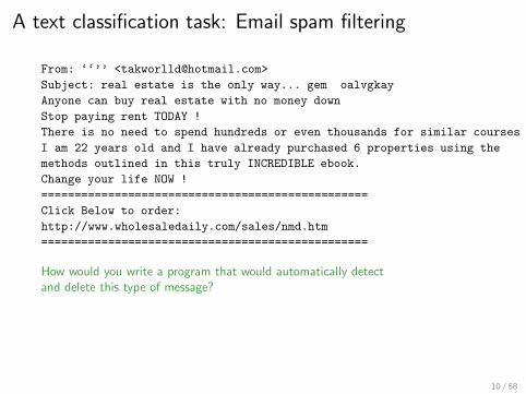
A text classification task: Email spam filtering

From: ‘‘’’ <takworlld@hotmail.com>

Subject: real estate is the only way... gem oalvgkay

Anyone can buy real estate with no money down

Stop paying rent TODAY !

There is no need to spend hundreds or even thousands for similar courses

I am 22 years old and I have already purchased 6 properties using the

methods outlined in this truly INCREDIBLE ebook.

Change your life NOW !

=================================================

Click Below to order:

http://www.wholesaledaily.com/sales/nmd.htm

=================================================

How would you write a program that would automatically detectand delete this type of message?

10 / 58

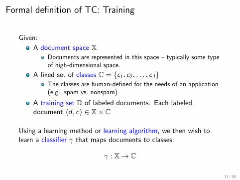
Formal definition of TC: Training

Given:

A document space X

Documents are represented in this space – typically some typeof high-dimensional space.

A fixed set of classes C = {c1, c2, . . . , cJ}

The classes are human-defined for the needs of an application(e.g., spam vs. nonspam).

A training set D of labeled documents. Each labeleddocument 〈d , c〉 ∈ X× C

Using a learning method or learning algorithm, we then wish tolearn a classifier γ that maps documents to classes:

γ : X→ C

11 / 58

Formal definition of TC: Application/Testing

Given: a description d ∈ X of a document Determine: γ(d) ∈ C,

that is, the class that is most appropriate for d

12 / 58

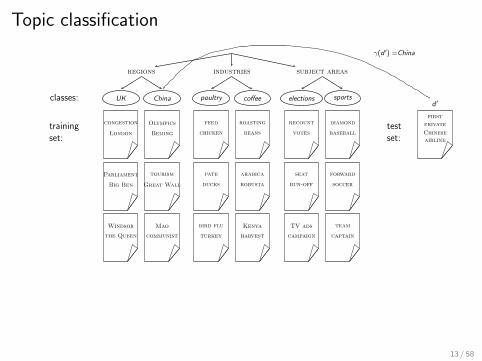
Topic classification

classes:

training

set:

test

set:

regions industries subject areas

γ(d ′) =China

first

private

Chinese

airline

UK China poultry coffee elections sports

London

congestion

Big Ben

Parliament

the Queen

Windsor

Beijing

Olympics

Great Wall

tourism

communist

Mao

chicken

feed

ducks

pate

turkey

bird flu

beans

roasting

robusta

arabica

harvest

Kenya

votes

recount

run-off

seat

campaign

TV ads

baseball

diamond

soccer

forward

captain

team

d ′

13 / 58

Exercise

Find examples of uses of text classification in informationretrieval

14 / 58

Examples of how search engines use classification

Language identification (classes: English vs. French etc.)

The automatic detection of spam pages (spam vs. nonspam)

Sentiment detection: is a movie or product review positive ornegative (positive vs. negative)

Topic-specific or vertical search – restrict search to a“vertical” like “related to health” (relevant to vertical vs. not)

15 / 58

Classification methods: 1. Manual

Manual classification was used by Yahoo in the beginning ofthe web. Also: ODP, PubMed

Very accurate if job is done by experts

Consistent when the problem size and team is small

Scaling manual classification is difficult and expensive.

→ We need automatic methods for classification.

16 / 58

Classification methods: 2. Rule-based

E.g., Google Alerts is rule-based classification.

There are IDE-type development enviroments for writing verycomplex rules efficiently. (e.g., Verity)

Often: Boolean combinations (as in Google Alerts)

Accuracy is very high if a rule has been carefully refined overtime by a subject expert.

Building and maintaining rule-based classification systems iscumbersome and expensive.

17 / 58

A Verity topic (a complex classification rule)

18 / 58

Classification methods: 3. Statistical/Probabilistic

This was our definition of the classification problem – textclassification as a learning problem

(i) Supervised learning of a the classification function γ and(ii) application of γ to classifying new documents

We will look at two methods for doing this: Naive Bayes andSVMs

No free lunch: requires hand-classified training data

But this manual classification can be done by non-experts.

19 / 58

Outline

1 Recap

2 Text classification

3 Naive Bayes

4 NB theory

5 Evaluation of TC

20 / 58

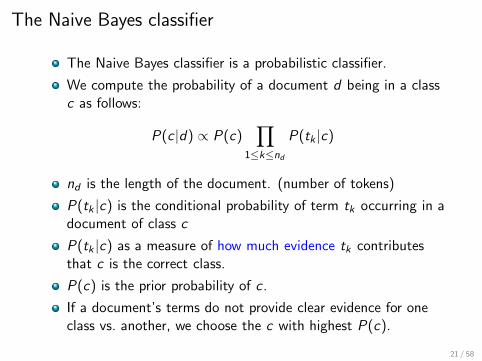
The Naive Bayes classifier

The Naive Bayes classifier is a probabilistic classifier.

We compute the probability of a document d being in a classc as follows:

P(c |d) ∝ P(c)∏

1≤k≤nd

P(tk |c)

nd is the length of the document. (number of tokens)

P(tk |c) is the conditional probability of term tk occurring in adocument of class c

P(tk |c) as a measure of how much evidence tk contributesthat c is the correct class.

P(c) is the prior probability of c .

If a document’s terms do not provide clear evidence for oneclass vs. another, we choose the c with highest P(c).

21 / 58

Maximum a posteriori class

Our goal in Naive Bayes classification is to find the “best”class.

The best class is the most likely or maximum a posteriori(MAP) class cmap:

cmap = argmaxc∈C

P(c |d) = argmaxc∈C

P(c)∏

1≤k≤nd

P(tk |c)

22 / 58

Taking the log

Multiplying lots of small probabilities can result in floatingpoint underflow.

Since log(xy) = log(x) + log(y), we can sum log probabilitiesinstead of multiplying probabilities.

Since log is a monotonic function, the class with the highestscore does not change.

So what we usually compute in practice is:

cmap = argmaxc∈C

[log P(c) +∑

1≤k≤nd

log P(tk |c)]

23 / 58

Naive Bayes classifier

Classification rule:

cmap = argmaxc∈C

[log P(c) +∑

1≤k≤nd

log P(tk |c)]

Simple interpretation:

Each conditional parameter log P(tk |c) is a weight thatindicates how good an indicator tk is for c .The prior log P(c) is a weight that indicates the relativefrequency of c .The sum of log prior and term weights is then a measure ofhow much evidence there is for the document being in theclass.We select the class with the most evidence.

24 / 58

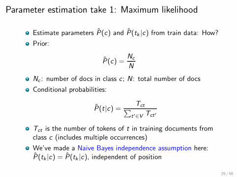
Parameter estimation take 1: Maximum likelihood

Estimate parameters P(c) and P(tk |c) from train data: How?

Prior:

P(c) =Nc

N

Nc : number of docs in class c ; N: total number of docs

Conditional probabilities:

P(t|c) =Tct∑

t′∈V Tct′

Tct is the number of tokens of t in training documents fromclass c (includes multiple occurrences)

We’ve made a Naive Bayes independence assumption here:P(tk |c) = P(tk |c), independent of position

25 / 58

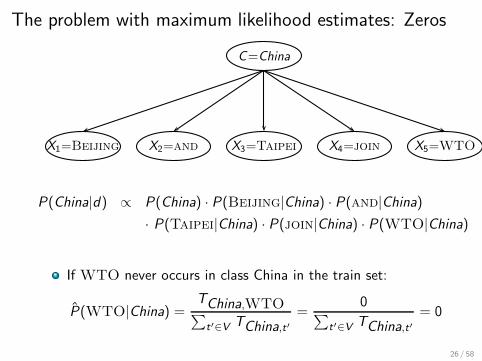
The problem with maximum likelihood estimates: Zeros

C=China

X1=Beijing X2=and X3=Taipei X4=join X5=WTO

P(China|d) ∝ P(China) · P(Beijing|China) · P(and|China)

· P(Taipei|China) · P(join|China) · P(WTO|China)

If WTO never occurs in class China in the train set:

P(WTO|China) =TChina,WTO∑t′∈V TChina,t′

=0∑

t′∈V TChina,t′= 0

26 / 58

The problem with maximum likelihood estimates: Zeros

(cont)

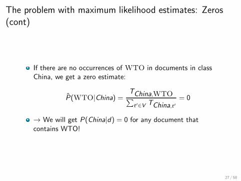
If there are no occurrences of WTO in documents in classChina, we get a zero estimate:

P(WTO|China) =TChina,WTO∑t′∈V TChina,t′

= 0

→ We will get P(China|d) = 0 for any document thatcontains WTO!

27 / 58

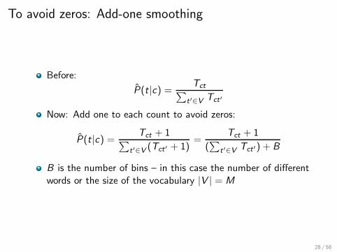
To avoid zeros: Add-one smoothing

Before:

P(t|c) =Tct∑

t′∈V Tct′

Now: Add one to each count to avoid zeros:

P(t|c) =Tct + 1∑

t′∈V (Tct′ + 1)=

Tct + 1

(∑

t′∈V Tct′) + B

B is the number of bins – in this case the number of differentwords or the size of the vocabulary |V | = M

28 / 58

Naive Bayes: Summary

Estimate parameters from the training corpus using add-onesmoothing

For a new document, for each class, compute sum of (i) log ofprior and (ii) logs of conditional probabilities of the terms

Assign the document to the class with the largest score

29 / 58

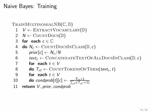
Naive Bayes: Training

TrainMultinomialNB(C,D)1 V ← ExtractVocabulary(D)2 N ← CountDocs(D)3 for each c ∈ C

4 do Nc ← CountDocsInClass(D, c)5 prior [c]← Nc/N6 textc ← ConcatenateTextOfAllDocsInClass(D, c)7 for each t ∈ V

8 do Tct ← CountTokensOfTerm(textc , t)9 for each t ∈ V

10 do condprob[t][c]← Tct+1∑t′(Tct′+1)

11 return V , prior , condprob

30 / 58

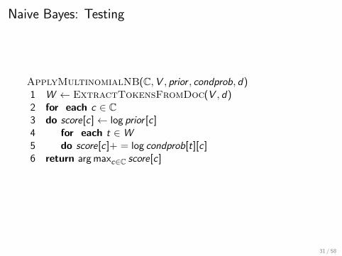
Naive Bayes: Testing

ApplyMultinomialNB(C,V , prior , condprob, d)1 W ← ExtractTokensFromDoc(V , d)2 for each c ∈ C

3 do score[c] ← log prior [c]4 for each t ∈W

5 do score[c]+ = log condprob[t][c]6 return argmaxc∈C score[c]

31 / 58

Exercise: Estimate parameters, classify test set

docID words in document in c = China?

training set 1 Chinese Beijing Chinese yes2 Chinese Chinese Shanghai yes3 Chinese Macao yes4 Tokyo Japan Chinese no

test set 5 Chinese Chinese Chinese Tokyo Japan ?

P(c) =Nc

N

P(t|c) =Tct + 1∑

t′∈V (Tct′ + 1)=

Tct + 1

(∑

t′∈V Tct′) + B

(B is the number of bins – in this case the number of different words or thesize of the vocabulary |V | = M)

cmap = argmaxc∈C

[P(c) ·∏

1≤k≤nd

P(tk |c)]

32 / 58

33 / 58

Example: Parameter estimates

Priors: P(c) = 3/4 and P(c) = 1/4 Conditional probabilities:

P(Chinese|c) = (5 + 1)/(8 + 6) = 6/14 = 3/7

P(Tokyo|c) = P(Japan|c) = (0 + 1)/(8 + 6) = 1/14

P(Chinese|c) = (1 + 1)/(3 + 6) = 2/9

P(Tokyo|c) = P(Japan|c) = (1 + 1)/(3 + 6) = 2/9

The denominators are (8 + 6) and (3 + 6) because the lengths oftextc and textc are 8 and 3, respectively, and because the constantB is 6 as the vocabulary consists of six terms.

34 / 58

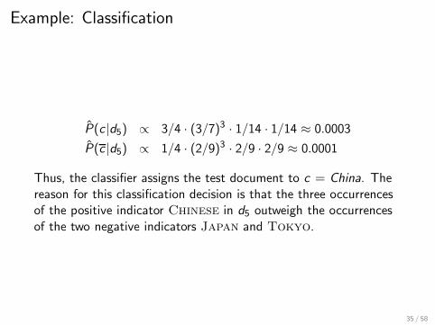
Example: Classification

P(c |d5) ∝ 3/4 · (3/7)3 · 1/14 · 1/14 ≈ 0.0003

P(c |d5) ∝ 1/4 · (2/9)3 · 2/9 · 2/9 ≈ 0.0001

Thus, the classifier assigns the test document to c = China. Thereason for this classification decision is that the three occurrencesof the positive indicator Chinese in d5 outweigh the occurrencesof the two negative indicators Japan and Tokyo.

35 / 58

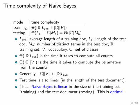
Time complexity of Naive Bayes

mode time complexity

training Θ(|D|Lave + |C||V |)testing Θ(La + |C|Ma) = Θ(|C|Ma)

Lave: average length of a training doc, La: length of the testdoc, Ma: number of distinct terms in the test doc, D:training set, V : vocabulary, C: set of classes

Θ(|D|Lave) is the time it takes to compute all counts.

Θ(|C||V |) is the time it takes to compute the parametersfrom the counts.

Generally: |C||V | < |D|Lave

Test time is also linear (in the length of the test document).

Thus: Naive Bayes is linear in the size of the training set(training) and the test document (testing). This is optimal.

36 / 58

Outline

1 Recap

2 Text classification

3 Naive Bayes

4 NB theory

5 Evaluation of TC

37 / 58

Naive Bayes: Analysis

Now we want to gain a better understanding of the propertiesof Naive Bayes.

We will formally derive the classification rule . . .

. . . and make our assumptions explicit.

38 / 58

Derivation of Naive Bayes rule

We want to find the class that is most likely given the document:

cmap = argmaxc∈C

P(c |d)

Apply Bayes rule P(A|B) = P(B|A)P(A)P(B) :

cmap = argmaxc∈C

P(d |c)P(c)

P(d)

Drop denominator since P(d) is the same for all classes:

cmap = argmaxc∈C

P(d |c)P(c)

39 / 58

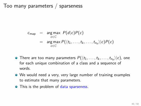
Too many parameters / sparseness

cmap = argmaxc∈C

P(d |c)P(c)

= argmaxc∈C

P(〈t1, . . . , tk , . . . , tnd 〉|c)P(c)

There are too many parameters P(〈t1, . . . , tk , . . . , tnd 〉|c), onefor each unique combination of a class and a sequence ofwords.

We would need a very, very large number of training examplesto estimate that many parameters.

This is the problem of data sparseness.

40 / 58

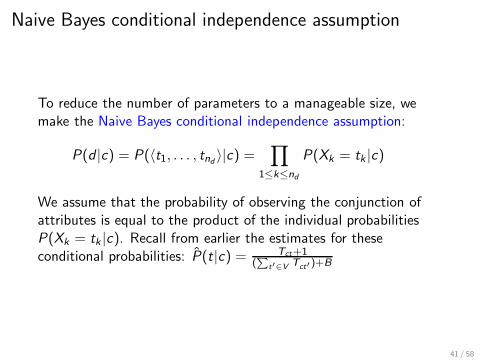
Naive Bayes conditional independence assumption

To reduce the number of parameters to a manageable size, wemake the Naive Bayes conditional independence assumption:

P(d |c) = P(〈t1, . . . , tnd 〉|c) =∏

1≤k≤nd

P(Xk = tk |c)

We assume that the probability of observing the conjunction ofattributes is equal to the product of the individual probabilitiesP(Xk = tk |c). Recall from earlier the estimates for theseconditional probabilities: P(t|c) = Tct+1

(∑

t′∈V Tct′)+B

41 / 58

Generative model

C=China

X1=Beijing X2=and X3=Taipei X4=join X5=WTO

P(c |d) ∝ P(c)∏

1≤k≤ndP(tk |c)

Generate a class with probability P(c)

Generate each of the words (in their respective positions),conditional on the class, but independent of each other, withprobability P(tk |c)

To classify docs, we “reengineer” this process and find theclass that is most likely to have generated the doc.

42 / 58

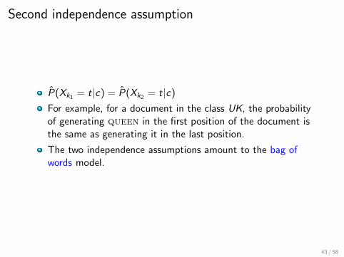
Second independence assumption

P(Xk1 = t|c) = P(Xk2 = t|c)

For example, for a document in the class UK, the probabilityof generating queen in the first position of the document isthe same as generating it in the last position.

The two independence assumptions amount to the bag ofwords model.

43 / 58

A different Naive Bayes model: Bernoulli model

UAlaska=0 UBeijing=1 U India=0 U join=1 UTaipei=1 UWTO=1

C=China

44 / 58

Violation of Naive Bayes independence assumptions

Conditional independence:

P(〈t1, . . . , tnd 〉|c) =∏

1≤k≤nd

P(Xk = tk |c)

Positional independence:

P(Xk1 = t|c) = P(Xk2 = t|c)

The independence assumptions do not really hold ofdocuments written in natural language.

Exercise

Examples for why conditional independence assumption is notreally true?Examples for why positional independence assumption is notreally true?

How can Naive Bayes work if it makes such inappropriateassumptions?

45 / 58

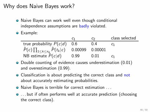
Why does Naive Bayes work?

Naive Bayes can work well even though conditionalindependence assumptions are badly violated.

Example:c1 c2 class selected

true probability P(c |d) 0.6 0.4 c1

P(c)∏

1≤k≤ndP(tk |c) 0.00099 0.00001

NB estimate P(c |d) 0.99 0.01 c1

Double counting of evidence causes underestimation (0.01)and overestimation (0.99).

Classification is about predicting the correct class and notabout accurately estimating probabilities.

Naive Bayes is terrible for correct estimation . . .

. . . but if often performs well at accurate prediction (choosingthe correct class).

46 / 58

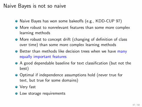
Naive Bayes is not so naive

Naive Bayes has won some bakeoffs (e.g., KDD-CUP 97)

More robust to nonrelevant features than some more complexlearning methods

More robust to concept drift (changing of definition of classover time) than some more complex learning methods

Better than methods like decision trees when we have manyequally important features

A good dependable baseline for text classification (but not thebest)

Optimal if independence assumptions hold (never true fortext, but true for some domains)

Very fast

Low storage requirements

47 / 58

Outline

1 Recap

2 Text classification

3 Naive Bayes

4 NB theory

5 Evaluation of TC

48 / 58

Evaluation on Reuters

classes:

training

set:

test

set:

regions industries subject areas

γ(d ′) =China

first

private

Chinese

airline

UK China poultry coffee elections sports

London

congestion

Big Ben

Parliament

the Queen

Windsor

Beijing

Olympics

Great Wall

tourism

communist

Mao

chicken

feed

ducks

pate

turkey

bird flu

beans

roasting

robusta

arabica

harvest

Kenya

votes

recount

run-off

seat

campaign

TV ads

baseball

diamond

soccer

forward

captain

team

d ′

49 / 58

Example: The Reuters collection

symbol statistic value

N documents 800,000L avg. # word tokens per document 200M word types 400,000

type of class number examples

region 366 UK, Chinaindustry 870 poultry, coffeesubject area 126 elections, sports

50 / 58

A Reuters document

51 / 58

Evaluating classification

Evaluation must be done on test data that are independent ofthe training data, i.e., training and test sets are disjoint.

It’s easy to get good performance on a test set that wasavailable to the learner during training (e.g., just memorizethe test set).

Measures: Precision, recall, F1, classification accuracy

52 / 58

Precision P and recall R

in the class not in the classpredicted to be in the class true positives (TP) false positives (FP)predicted to not be in the class false negatives (FN) true negatives (TN)

TP, FP, FN, TN are counts of documents. The sum of these four

counts is the total number of documents.

precision:P = TP/(TP + FP)

recall:R = TP/(TP + FN)

53 / 58

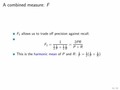
A combined measure: F

F1 allows us to trade off precision against recall.

F1 =1

121P+ 1

21R

=2PR

P + R

This is the harmonic mean of P and R : 1F= 1

2(1P+ 1

R)

54 / 58

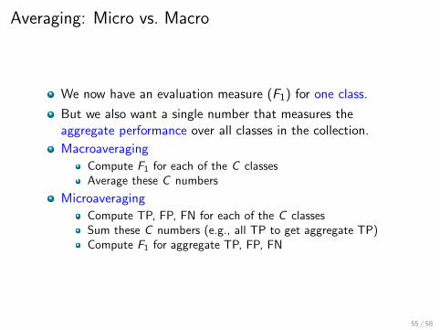
Averaging: Micro vs. Macro

We now have an evaluation measure (F1) for one class.

But we also want a single number that measures theaggregate performance over all classes in the collection.

Macroaveraging

Compute F1 for each of the C classesAverage these C numbers

Microaveraging

Compute TP, FP, FN for each of the C classesSum these C numbers (e.g., all TP to get aggregate TP)Compute F1 for aggregate TP, FP, FN

55 / 58

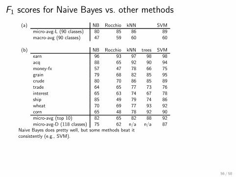
F1 scores for Naive Bayes vs. other methods

(a) NB Rocchio kNN SVMmicro-avg-L (90 classes) 80 85 86 89macro-avg (90 classes) 47 59 60 60

(b) NB Rocchio kNN trees SVMearn 96 93 97 98 98acq 88 65 92 90 94money-fx 57 47 78 66 75grain 79 68 82 85 95crude 80 70 86 85 89trade 64 65 77 73 76interest 65 63 74 67 78ship 85 49 79 74 86wheat 70 69 77 93 92corn 65 48 78 92 90micro-avg (top 10) 82 65 82 88 92micro-avg-D (118 classes) 75 62 n/a n/a 87

Naive Bayes does pretty well, but some methods beat itconsistently (e.g., SVM).

56 / 58

Take-away today

Text classification: definition & relevance to informationretrieval

Naive Bayes: simple baseline text classifier

Theory: derivation of Naive Bayes classification rule & analysis

Evaluation of text classification: how do we know it worked /didn’t work?

57 / 58

Resources

Chapter 13 of IIR

Resources at http://cislmu.org

Weka: A data mining software package that includes animplementation of Naive BayesReuters-21578 – text classification evaluation setVulgarity classifier fail

58 / 58