Introduction to Homogenization Theory -

Periodic Second Order Elliptic Equations

Yi-Hsuan Lin

Abstract

The note is mainly for personal record, if you want to readit, please be careful. This notes was given by Prof. Zhongwei Shen’slecture in the National Taiwan University, 2015.03. For more details werefer readers to his draft lecture (with a similar title as this lecture).For simplicity, the following arguments hold for the linear elliptic system,however, we only discuss the linear scalar elliptic equation case in thislecture.

1 Introduction

We consider the following elliptic equations−∆u = F in Ω ⊂ Rd,−∇ · (A(x)∇u) = F in Ω ⊂ Rd,F (D2u,Du, u, x) = F in Ω ⊂ Rd,

with suitable boundary conditions.

Medium with a fine self-similar microscopic structure. Let ε > 0 be a smallparameter, and consider the following homogenization problem

F (D2uε, Duε, uεx

ε, x) = 0 in Ω, with suitable boundary conditions.

In the following, we only consider the simplest linear elliptic homogenization

problem. Let A(x) = (aij(x))d×d, Aε(x) = A(

x

ε) and consider

−∇ · (A(

x

ε)∇uε) = F in Ω,

Suitable boundary condition on ∂Ω.(1)

What can we say about uε as ε→ 0. In fact, we have

uε u0 weakly in H1(Ω) and uε → u0 strongly in L2(Ω).

As a result, for F ∈ H−1(Ω), we have−∇ · (A(

x

ε)∇uε) = F in Ω,

Suitable B.Cs−→

−∇ · (A∇u0) = F in Ω,

Same B.Cs

1

as ε → 0 and A = (aij)d×d is a constant matrix. Here is the problem setting.Assume the second order elliptic operator

Lε := − ∂

∂xiaij(

x

ε)∂

∂xj

with the coefficients satisfyingEllipticity: µ|ξ|2 ≤ aij(y)ξiξj ≤1

µ|ξ|2, for all ξ ∈ Rd,

1-Periodicity: A(y + z) = A(y) for all y ∈ Rd, z ∈ Zd.

Consider the Dirichlet problem to beLεuε = F in Ω,

uε = g on ∂Ω,(2)

where F ∈ H−1(Ω), g ∈ H1/2(∂Ω), and Ω is a bounded Lipschitz domain in Rd.By the Lax-Milgram lemma, we have

‖uε‖H1(Ω) ≤ C‖F‖H−1(Ω) + ‖g‖H1/2(∂Ω), (3)

where the constant C independent of ε. Note that uε is a weak solution of (2)if for all ϕ ∈ H1

0 (Ω), we haveˆ

Ω

(A(x

ε)∇uε) · ∇ϕdx = 〈F,ϕ〉H−1(Ω)×H1

0 (Ω) .

Consider the Neumann problem to beLεuε = F in Ω,∂uε∂νε

= g on ∂Ω,(4)

where F ∈ H−10 (Ω) = (H1(Ω))′, g ∈ H−1/2(∂Ω) = (H1/2(∂Ω))′,

∂uε∂νε

=

νi(x)aij(x

ε)∂uε∂xj

, and ν = (ν1, ν2, · · · , νd) is a unit outer normal on ∂Ω. Simi-

larly, we call uε to be a weak solution if for all ϕ ∈ H1(Ω), we haveˆ

Ω

(A(x

ε)∇uε) · ∇ϕdx = 〈F,ϕ〉H−1(Ω)×H1

0 (Ω) − 〈g, ϕ〉H−1/2(∂Ω)×H1/2(∂Ω) .

Moreover, by the Lax-Milgram lemma again, we have

‖∇uε‖L2(Ω) ≤ C‖F‖H−10 (Ω) + ‖g‖H−1/2(∂Ω), (5)

where C is independent of ε. For the second order elliptic system, we considerthe homogenization problem to beLεuε = − ∂

∂xi

[aαβij (

x

ε)∂uβε∂xj

]= Fα in Ω

uε satisfies suitable boundary conditions

with 1 ≤ i, j ≤ d and 1 ≤ α, β ≤ m. In order to demonstrate ideas, we considerm = 1 in most situations.

2

2 Derivation of the homogenized equation

The ideas of the derivation of the homogenized equation is quite clever. Weconsider uε to be the perturbation of u0 with respect to ε-parameter. Moreover,by observing the elliptic operator Lε, we introduce the two-scaled method, which

means we consider x = x, and y =x

εto be two independent parameters. Let

uε := u0 + εu1 + ε2u2 + · · ·

be the asymptotic expansion of uε, where

uj := uj(x, y) = uj(x,x

ε).

In addition,

∇uj = ∇xuj(x, y) +1

ε∇yuj(x, y), as y =

x

ε,

which means under our two-scaled method, the operator ∇ = ∇x+1

ε∇y. There-

fore, (1) will become

− (∇x +1

ε∇y) · A(y)[(∇x +

1

ε∇y)(u0 + εu1 + ε2u2 + · · · )] = F (x) in Ω, (6)

where we are not concerned about the boundary condition for the equation.Expand (6) and compare it with the same orders, so we get

O(1

ε2) : −∇y · (A(y)∇yu0(x, y)) = 0,

O(1

ε) : −∇y · (A(y)∇yu1(x, y)) = ∇y · (A(y)∇xu0) +∇x · (A(y)∇yu0),

O(1) : −∇y · (A(y)∇yu2(x, y)) = ∇y · (A(y)∇xu1) +∇x · (A(y)∇yu1)

+∇x · (A(y)∇xu0) + F (x).

Recall that for the periodic elliptic equation

−∇ · (A(y)∇u(y)) = h(y), A(y) is 1-periodic,

then we have ˆTdh(y)dy = 0

by using the Stokes formula. For O(1

ε2) term, this equation is solvable because

the right hand side is zero. In further, we multiply u0(x, y) on both sides andintegrate by parts, which will imply

0 =

ˆTdA(y)∇yu0 · ∇yu0 ≥ µ

ˆTd|∇yu0(x, y)|2dy ≥ 0,

which gives us the information that

u0(x, y) ≡ u0(x)

3

independent of y.

Now, for the second term O(1

ε), the second term on the right hand side

should be zero since ∇yu0(x) = 0. Solve the equation

−∇y · (A(y)∇yu1(x, y)) = ∇y · (A(y)∇xu0)

= (∇y ·A(y))(∇xu0)

formally. Note that since A(y) is 1-periodic, then the equation is solvable foru1 if ˆ

Td(∇y ·A(y))∇xu0)dy =

ˆ∂Td

(A(y)∇xu0) · ν(y)dS(y) = 0.

By using the separation of variables, we put the ansatz

u1(x, y) = χ(y)(∇xu0(x))

into the equation with χ(y) being 1-periodic, we will find that

−∇ · (A(y)∇yχ(y))(∇xu0) = (∇y ·A(y))(∇xu0).

Moreover, we call−∇ · (A(y)∇yχ(y)) = (∇y ·A(y))

to be the cell problem and χ(y) to be the corrector.Finally, we observe the last equation carefully. Put u1(x, y) = χ(y)∇xu0

into the O(1) equation and examine the solvability condition for u2(x, y), wehave

0 =

ˆTd

[∇y · (A(y)∇xu1) +∇x · (A(y)∇yu1) +∇x · (A(y)∇xu0) + F (x)]dy

= ∇x · [ˆTdA(y)(∇yχ(y))dy]∇xu0+∇x · [

ˆTdA(y)dy]∇xu0+ F (x),

where the first term vanishes by the periodicity of A and χ. Thus, we can obtain

−∇ · (A∇u0) = F (x) in Ω, (7)

where

A =

ˆTdA(y) +A(y)(∇yχ(y))dy

is the (constant) homogenized operator and we call (7) to be the homogenizedequation. For the rigorous derivation of the homogenized equation, we will givethe serious proof later by using the famous tool: The Div-Curl lemma.

3 Basic properties

Now, let us recall the corrector again. χ = (χ1, χ2, · · · , χd) ∈ H1per(Zd) is the

corrector, where H1per(Zd) is the closure of C∞ 1-periodic function under the

standard H1-norm. We rewrite the cell problem in the following way:−∂

∂yiaij(y)

∂χk∂yj =

∂

∂yi(aik(y)) in Rd,

χk ∈ H1per(Zd), 1 ≤ k ≤ d.

4

Note that∂

∂yi(aik(y)) =

∂

∂yi(aij(y)

∂

∂yj(yk)), then the cell-problem becomes

L1(χk + xk) = 0 in Rd.

In addition, we consider the equivalence space H1per(Zd)/ ∼ and define the

bilinear form

aper(φ, ψ) :=

ˆTdaij(y)

∂φ

∂yj

∂ψ

∂yidy,

then we also can prove the Lax-Milgram lemma under this equivalence Sobolevspace. Moreover, when φ ∈ H1

per(Zd), then aper(u, φ) = 0 for all u ∈ H1(Ω).

For convenience, we set L0 := −∇ · (A∇) be the homogenized second orderelliptic operator with respect to A.

Proposition 3.1. The homogenized operator A = (aij)can be rewritten in thefollowing form

aij = aper(yj + χj , yi).

Moreover, use the above relation, we can write A as

aij = aper(yj + χj , yi + χi).

Use the above proposition, it is not hard to obtain the following theorem.

Theorem 3.2. L0 is elliptic, which means

µ|ξ|2 ≤ aijξiξj ≤ µ1|ξ|2,

where the lower bound comes from the original A, and µ1 = µ1(µ, d).

Proof. aij = aper(yj + χj , yi + χi) and aper(yj + χj , φ) = 0 when φ ∈ H1per(Zd).

Therefore, we have

aijξiξj = aper((yj + χj)ξj , (yi + χi)ξi)

≥ µˆZd|∇(χi + yi)ξi|2dy

=

ˆTd|∇(χiξi)|2 + 2∇(χiξi) · ∇(yiξi) + |∇(yiξi)|2

≥ µ|ξ|2,

since ∇(χiξi) · ∇(yiξi) = 0.

For the rigorous proof of the Lε → L0 in a suitable sense, we use the followingtwo useful lemmas.

Lemma 3.3. Let h ∈ L2loc(Rd) and 1-periodic, then

h(x

ε) c0 :=

ˆTdh(y)dy

weakly in L2(Ω).

5

Proof. We gave a hint for readers and leave details of proof to an exercise. Hint:Try to solve

∆u = h in Td,u is 1-periodic.

Lemma 3.4. (Div-Curl lemma) Let uk, vk be two bounded sequences inL2(Ω,Rd). Suppose that uk u0, vk v0 weakly in L2(Ω,Rd) and ∇×uk = 0for all k, ∇ · vk → f strongly in H−1(Ω). Thenˆ

Ω

uk · vkϕdx→ˆ

Ω

u0 · v0ϕdx

for all ϕ ∈ C10 (Ω).

Proof. Leave this lemma to an exercise.

Theorem 3.5. (Homogenization Theorem) Suppose A(y) is elliptic and 1-periodic. Let Ω be a bounded Lipschitz domain. If uε is a weak solution ofthe Dirichlet problem (2). Then uε u0 weakly in H1(Ω) and strongly inL2(Ω), where u0 ∈ H1(Ω) is the weak solution to the homogenized equation

L0u0 = F in Ω,

u0 = g on ∂Ω.

Moreover, we have A(x

ε)∇uε A∇u0 weakly in L2(Ω,Rd).

Remark 3.6. In general, uε does not converge to u0 strongly in H1(Ω).

Before giving proofs for the homogenization theorem, we introduce the dual

problem for the homogenization problem. Let L∗ε := −∇ · (A∗(xε

)∇) be the

adjoint operator of Lε. Then we have the following properties.

1. a∗ij = aji.

2. a∗per(φ, ψ) = aper(ψ, φ).

3. Let χ∗ be the corrector of L∗ε , then we have

a∗per(yk + χ∗k, ψ) = 0, for all ψ ∈ H1per(Zd).

Proposition 3.7. We have aij = a∗per(yi + χi, yi) and A∗

= A∗. If A = A∗,

then A∗

= A.

Proof. Exercise.

In addition, we have

aij = a∗per(yi + χi, yj) = aper(yj , yi + χ∗i )

=

ˆTda`k(y)

∂yj∂yk

∂(yi + χ∗i )

∂y`dy

=

ˆTda`j(y)δ`k +

∂χ∗i∂y`dy

=

ˆTdaij(y) + a`j(y)

∂χ∗i∂y`dy.

6

Now we prove the theorem.

Proof. By using the Lax-Milgram theorem, we have

‖uε‖H1(Ω) ≤ C‖F‖H−1(Ω) + ‖g‖H1/2(∂Ω),

which means uε is bounded in H1(Ω). Moreover, uε satisfies (2) and

ˆΩ

A(x

ε)∇uε · ϕdx = 〈F,ϕ〉 .

By the duality argument, we have ‖A(x

ε)∇uε‖L2(Ω) ≤ C <∞. WLOG, we say

uε be the sequence such that uε v weakly in H1(Ω) and A(x

ε)∇uε to p

weakly in L2(Ω). Then remaining work is to provev = u0 and

p = A∇u0.

ConsiderˆΩ

A(x

ε)∇uε · ∇(xk + εχ∗k(

x

ε))ψdx =

ˆΩ

∇uε ·A∗(x

ε)∇(xk + εχ(

x

ε))ψdx,

for all ψ ∈ C10 (Ω). For the left side, we have A(

x

ε)∇uε p weakly in L2(Ω;Rd).

∇(xk + εχ∗k(x

ε)) = δik +

∂χ∗k∂xi

(x

ε)L2

δik +

ˆTd

∂χ∗k∂yi

dy = δik,

and∇× (∇(xk + εχ∗k(

x

ε)) = 0 and ∇ · (A(

x

ε)∇uε) = F.

The left hand side satisfies conditions of the Div-Curl lemma, then the left handside will converge to ˆ

Ω

piδikψdx =

ˆΩ

pkψdx.

For the right side, ∇uε ∇u0 in L2,

A∗(x

ε)∇(xk + εχ∗k(

x

ε)) = A∗(

x

ε)∇xk +∇χ∗k(

x

ε)

ˆTda∗ij(y)δjk +

∂

∂yj(χ∗k)dy

=

ˆZdaki(y) + aji(y)

∂χ∗k∂yjdy

= aki.

Then the right side converges to´

Ω

∂v

∂xiakiψdx. Thus,

´Ωpkψdx =

´Ω

∂v

∂xiakiψdx,

which implies

pk = aki∂v

∂xiand A(

x

ε)∇uε A∇v

7

and −∇ · (A∇v) = F in Ω,

v = g on ∂Ω,

and v = u0 (uniqueness for Dirichlet problem).

Remark 3.8. The homogenization theorem still holds for the Neumann problemLε(uε) = F in Ω,∂uε∂νε

= g on ∂Ω,

where F ∈ H−10 (Ω), g ∈ H−1/2(∂Ω), and

´Ωuε = 0. The proof is followed by

using ˆΩ

A(x

ε)∇uε · ∇ψdx = 〈F,ψ〉H−1

0 ×H1 − 〈g, ψ〉H−1/2×H1/2 ,

and use the Div-Curl lemma argument, then we can obtain the desired results.

4 Rates of convergence

In the homogenization theory, it is interesting that how fast for uε convergingto u0.

Theorem 4.1. (Dirichlet) Suppose A is elliptic and 1-periodic. Let Ω be abounded Lipschitz domain. Then

‖uε − u0 − εχ(x

ε) · ∇u0‖H1(Ω) ≤ C

√ε‖u0‖W 2,d(Ω).

If d ≥ 3 and χ is Holder continuous (if m = 1),

‖uε − u0 − εχ(x

ε) · ∇u0‖H1(Ω) ≤ C

√ε‖u0‖W 2,2(Ω).

From ‖uε − u0 − εχ(x

ε)∇u0‖ ≤ C

√ε‖u0‖W 2,d(Ω), we can derive

‖uε − u0‖L2(Ω) ≤ ε‖χ(x

ε)∇u0‖L2(Ω) + C

√ε‖u0‖W 2,d(Ω)

≤ C√ε‖u0‖W 2,d(Ω).

Notice that the second inequality is nontrivial, we leave it as an exercise toreaders. Moreover, we have

‖uε − u0‖L2(Ω) ≤ Cε‖u0‖W 2,2(Ω) if

Ω is Lipschitz, m = 1,

Ω is C1,1, m ≥ 2,

and

‖uε − u0‖H1/2(Ω) ≤ Cε‖u0‖W 2,2(Ω), when coefficients are Holder continuous.

Definition 4.2. Define bij(y) := aij(y) + aik(y)∂χj∂yk− aij .

8

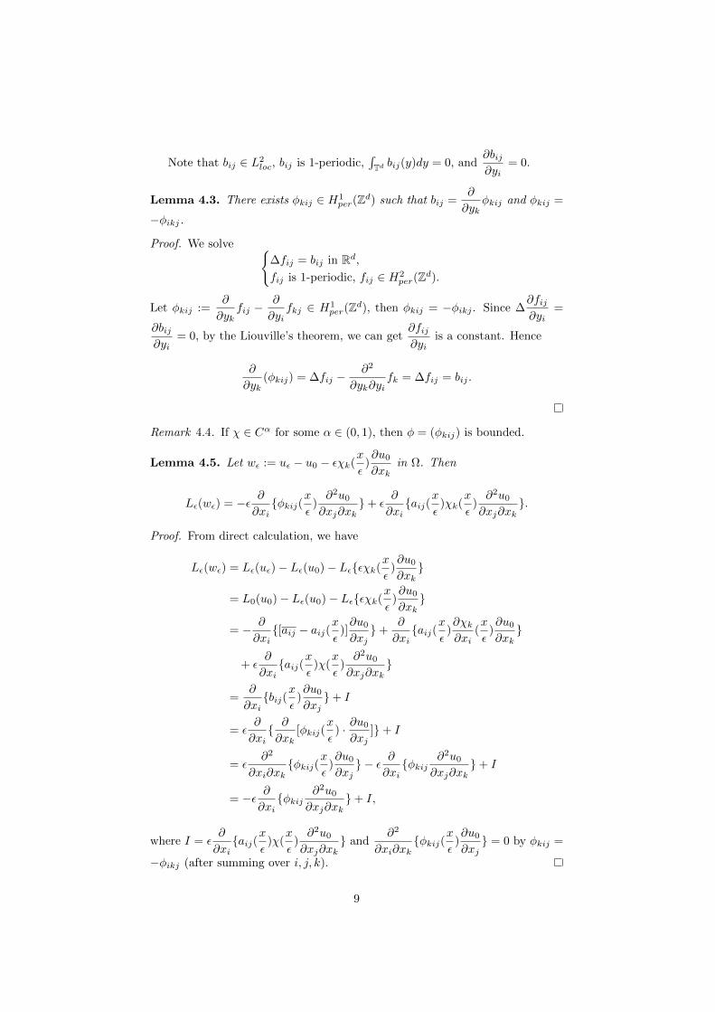
Note that bij ∈ L2loc, bij is 1-periodic,

´Td bij(y)dy = 0, and

∂bij∂yi

= 0.

Lemma 4.3. There exists φkij ∈ H1per(Zd) such that bij =

∂

∂ykφkij and φkij =

−φikj.

Proof. We solve ∆fij = bij in Rd,fij is 1-periodic, fij ∈ H2

per(Zd).

Let φkij :=∂

∂ykfij −

∂

∂yifkj ∈ H1

per(Zd), then φkij = −φikj . Since ∆∂fij∂yi

=

∂bij∂yi

= 0, by the Liouville’s theorem, we can get∂fij∂yi

is a constant. Hence

∂

∂yk(φkij) = ∆fij −

∂2

∂yk∂yifk = ∆fij = bij .

Remark 4.4. If χ ∈ Cα for some α ∈ (0, 1), then φ = (φkij) is bounded.

Lemma 4.5. Let wε := uε − u0 − εχk(x

ε)∂u0

∂xkin Ω. Then

Lε(wε) = −ε ∂

∂xiφkij(

x

ε)∂2u0

∂xj∂xk+ ε

∂

∂xiaij(

x

ε)χk(

x

ε)∂2u0

∂xj∂xk.

Proof. From direct calculation, we have

Lε(wε) = Lε(uε)− Lε(u0)− Lεεχk(x

ε)∂u0

∂xk

= L0(u0)− Lε(u0)− Lεεχk(x

ε)∂u0

∂xk

= − ∂

∂xi[aij − aij(

x

ε)]∂u0

∂xj+

∂

∂xiaij(

x

ε)∂χk∂xi

(x

ε)∂u0

∂xk

+ ε∂

∂xiaij(

x

ε)χ(

x

ε)∂2u0

∂xj∂xk

=∂

∂xibij(

x

ε)∂u0

∂xj+ I

= ε∂

∂xi ∂

∂xk[φkij(

x

ε) · ∂u0

∂xj]+ I

= ε∂2

∂xi∂xkφkij(

x

ε)∂u0

∂xj − ε ∂

∂xiφkij

∂2u0

∂xj∂xk+ I

= −ε ∂

∂xiφkij

∂2u0

∂xj∂xk+ I,

where I = ε∂

∂xiaij(

x

ε)χ(

x

ε)∂2u0

∂xj∂xk and

∂2

∂xi∂xkφkij(

x

ε)∂u0

∂xj = 0 by φkij =

−φikj (after summing over i, j, k).

9

For more delicate rates of convergence, we introduce the boundary corrector.Let vε be a solution satisfyingLε(vε) = 0 in Ω,

vε = −χk(x

ε)∂u0

∂xkon ∂Ω,

then we have the following theorem.

Theorem 4.6. For d ≥ 3, we have

‖uε − u0 − εχk(x

ε)∂u0

∂xk− εvε‖H1

0 (Ω) ≤ Cε‖∇2u0‖Ld(Ω).

Proof. (Sketch) Let wε := uε−u0− εχk(x

ε)∂u0

∂xk− εvε, then it is easy to see that

wε ∈ H10 (Ω) and Lε(wε) = Lε(wε). Hence by the Lax-Milgram lemma, we have

‖wε‖H10 (Ω) ≤ C‖Lε(wε)‖H−1(Ω)

≤ Cε‖φ(x

ε)∇2u0‖L2(Ω) + ‖χ(

x

ε)∇2u0‖L2(Ω).

The remaining task is to estimate

‖φ(x

ε)∇2u0‖L2(Ω) + ‖χ(

x

ε)∇2u0‖L2(Ω) ≤ Cε‖∇2u0‖Ld(Ω).

For the first term, we have

ˆΩ

|φ(x

ε)∇2u0|2dx ≤

ˆΩ

|φ(x

ε)|2|∇2u0|2dx

≤ (

ˆΩ

|φ(x

ε)|

2dd−2 dx)

d−2d (

ˆΩ

|∇2u0|ddx)2d .

Note that∇φ ∈ L2(Td) and the Sobolev embedding theorem gives´Td |φ|

2dd−2 dx ≤

C´Td |∇φ|

2dx ≤ C and

ˆΩ

|φ(x

ε)|

2dd−2 dx ≤

ˆ1εΩ

|φ(y)|2dd−2 dy · εd ≤ C.

For the other term, we leave it to readers.

Remark 4.7. If d = 2, χ ∈ Cα for some α ∈ (0, 1), then we can use the MeyersLp estimate to derive φ ∈ L∞(Td).

Now, we want to prove the fact that

‖uε − u0 − εχ(x

ε)∇u0‖H1(Ω) ≤ C

√ε‖u0‖W 2,d(Ω). (8)

To prove (8), only need to check the following lemma.

Lemma 4.8. ‖vε‖H1(Ω) ≤C√ε‖u0‖W 2,d(Ω).

10

Proof. Recall that vε satisfiesLε(vε) = 0 in Ω,

vε = −χk(x

ε)∂u0

∂xkon ∂Ω,

and by the standard elliptic regularity, we have

‖vε‖H1(Ω) ≤ C‖χk(x

ε)∂u0

∂xk‖H1/2(∂Ω) ≤ C‖ηε(x)χk(

x

ε)∂u0

∂xk‖H1(Ω),

where ηε ∈ C10 (Rd) with ηε(x) =

1, if dist(x, ∂Ω) ≤ ε0, if dist(x, ∂Ω) ≥ 2ε

, and ‖∇ηε‖L∞ ≤C

ε.

Therefore, we haveˆΩ

|∇ηε|2|χ(x

ε)|2|∇u0|2dx

≤Cε2

ˆdist(x,∂Ω)≤2ε

|χ(x

ε)|2|∇u0|2dx

≤Cε2

(

ˆdist(x,∂Ω)≤2ε

|χ(x

ε)|

2dd−2 |dx)

d−2d (

ˆdist(x,∂Ω)≤2ε

|∇u0|d)2d .

Claim:´dist(x,∂Ω)≤2ε

|χ(x

ε)|

2dd−2 dx ≤ Cε and

´dist(x,∂Ω)≤2ε

|∇u0|ddx ≤ Cε‖u0‖dW 2,d(Ω)

(this is true ∀u0 ∈W 2,d(Ω)).For the first part, we choose cubes Qεj with diamQεj ∼ O(ε) and

dist(x, ∂Ω) ≤ 2ε ⊂ ∪Nj=1Qεj ⊂ dist(x, ∂Ω) ≤ 5ε.

We can estimate χ in each cubes and use the periodicity of χ, we can find theuniform estimate for the first term.

For the second part, let Ωt := x ∈ Ω; dist(x, ∂Ω) > t and n be the unitouter normal on ∂Ωt. Let C0 > 0 be a positive constant and −→α be the vectorsuch that 〈n,−→α 〉 ≥ C0 > 0. Then

C0

ˆ∂Ωt

|∇u0|qdS ≤ˆ

Ωt

|∇u0|q 〈n,−→α 〉 dS

≤ˆ

Ωt

div−→α |∇u0|qdx+ αk∂

∂xk(|∇u0|q)dx

≤Cˆ

Ωt

|∇u0|qdx+ C

ˆΩt

|∇u0|q−1|∇2u0|dx

≤C‖u0‖qW 2,q .

Finally, integrate the above inequalities by´ 2ε

0dt, then we can obtain the desired

estimate and the constant C is independent of ε. Combine the above estimatestogether, we will find

‖uε − u0‖L2(Ω) ≤ C√ε‖u0‖W 2,d(Ω).

Remark 4.9. In fact, we can prove

‖uε − u0‖L2(Ω) ≤ Cε‖u0‖W 2,2(Ω) if

Ω is Lipschitz, m = 1,

Ω is C1,1, m ≥ 2.

11

5 Construction of Dirichlet corrector

Let Φε = (Φε,j) ∈ H1(Ω) be the Dirichlet corrector satisfyingLε(Φε,j) = 0 in Ω,

Φε,j = xj on ∂Ω.(9)

Note that xj itself also satisfies (9).

Proposition 5.1. Assume that m = 1, then

‖Φε,j − xj‖L∞(Ω) ≤ Cε.

Proof. Let uε = xj + εχj(x

ε)− Φε,j(x), thenLε(uε) = Lε(xj + εχj(

x

ε))− Lε(Φε,j) = 0 in Ω,

uε = εχj(x

ε) on ∂Ω.

By the maximum principle, we have

‖uε‖L∞(Ω) ≤ ‖uε‖L∞(∂Ω) = ε‖χj(x

ε)‖L∞(∂Ω)

≤ ε‖χj(x

ε)‖L∞(∂Ω) ≤ Cε,

which implies

‖Φε,j − xj‖∞ ≤ ‖uε‖∞ + ‖εχj(x

ε)‖∞ ≤ Cε.

Remark 5.2. When m ≥ 2, we consider

wε = uε − u0 − εχk(x

ε)Sε(

∂u0

∂xk),

where u0 is an extension of u0 to Rd by 0 outside Ω, and Sε(u0)(x) =fflBε(x)

u0 is

called the Steklov smoothing operator (the ideas were discovered by A. Suslina).

6 Uniform interior estimates

The uniform estimates are given by the compensated compactness argument.

Theorem 6.1. Suppose A = A(y) is elliptic and periodic. Let uε ∈ H1(B(x0, R))be a weak solution of Lε(uε) = F in B = B(x0, R). Suppose that F ∈ Lp(B),p > d and 0 < ε < R, then

(

B

|∇uε|2)1/2 ≤ C( B

|∇uε|2)1/2 +R(

B

|F |p)1/2,

where Cp = C(d, p, µ).

12

Theorem 6.2. (M. Avellenda, F. H. Lin, 1987) Suppose A = A(y) is ellipticand periodic. A(y) satisfies

|A(y)−A(z)| ≤ λ|y − z|τ , ∀y, z ∈ Rd, for some τ > 0.

Let uε ∈ H1(B) be a weak solution of Lε(uε) = F in B = B(x0, R), whereF ∈ Lp(B), p > d. Then

|∇uε(x0)| ≤ Cp( B

|∇uε|2)1/2 +R(

B

|F |p)1/p,

or

‖∇uε‖L∞(BR/2) ≤ Cp( B

|∇uε|2)1/2 +R(

B

|F |p)1/p,

where Cp = C(p, d, µλ, τ).

Observations:

1. Translation.If −∇ · (A(

x

ε)∇uε) = F and vε = uε(x− x0), then

−∇ · (A(x

ε)∇vε) = F ,

where A(y) = A(y +x0

ε) and F = F (x− x0).

2. Dilation.If −∇ · (A(

x

ε)∇uε) = F and vε(x) = uε(rx), r > 0, then

L εr(vε) = G,

where G(x) = r2F (rx).

Note that Theorem 1 implies Theorem 2 by using the blow-up arguments. Bytranslation and dilation, we may assume x0 = 0 and R = 1. Also, we may

assume ε <1

2(if ε ≥ 1

2, then A(

x

ε) is good, we only need to use the standard

argument for elliptic regularity).

Let wε(x) = ε−1uε(εx), then L1(w) = εF (εx) in B(0, 1) (note that1

ε> 1).

By the interior Lipschitz estimates for L1, we have

|∇w(0)| ≤ C( B(0,1)

|∇w|2)1/2 + (

B(0,1)

|εF (εx)|p)1/p.

This implies

|∇uε(0)| ≤ C( B(0,ε)

|∇uε|2)1/2 + ε(

B(0,ε)

|F |p)1/p

≤ C( B(0,ε)

|∇uε|2)1/2 + ε1−dp (

B(0,1)

|F |p)1/p

≤ C( B(0,1)

|∇uε|2)1/2 + (

B(0,1)

|F |p)1/p.

13

Remark 6.3. Local property needs the regularity, but the global one does notin the homogenization theory.

Theorem 6.4. (Compactness) Let A`(y) be a sequence of 1-periodic matrices

satisfying the elliptic condition with the same µ. Suppose −∇·(A`( xε`

)∇u`) = F`

in Ω, where ε` → 0. Also assume that u` → u in H1(Ω), A` → A0, and F` → F

in H−1(Ω). Then A`(x

ε`)∇u` A0∇u weakly in L2(Ω) and −∇ · (A0∇u) = F

in Ω.

Proof. The proof is similar to the proof of the homogenization theorem.

7 Compensated compactness

Here we give the compactness argument, which contains three steps. The firstis one-step improvement, the second is iteration, the last is blow-up argument.

Lemma 7.1. (One-step improvement) Let 0 < σ < ρ < 1 and ρ = 1− dp

. There

exist ε0 ∈ (0,1

2) and θ ∈ (0,

1

4) depending on µ, σ, ρ, d such that

(

B(0,θ)

|uε − B(0,θ)

uε − xj + εχj(x

ε))

B(0,θ)

∂uε∂xj|2)1/2

≤θ1+σ max( B(0,1)

|uε|2)1/2, (

B(0,1)

|F |p)1/p,

where 0 < ε < ε0, uε ∈ H1(B(0, 1)) is a solution of Lε(uε) = F in B(0, 1).

Proof. Prove it by contradiction. Use the fact that if −∇ · (A0∇u) = F in

B(0,1

2), then

sup|x|<θ

|u− B(0,θ)

u− xj B(0,θ)

∂u

∂xj| ≤ Cθ1+ρ‖∇u‖C0,ρ(B(0,θ))

≤ Cθ1+ρ‖∇u‖C0,ρ(B(0, 14 ))

≤ C0θ1+ρ max(

B(0, 12 )

|u|2)1/2, (

B(0, 12 )

|F |p)1/p.

Since σ < ρ, choose θ ∈ (0,1

4) such that 2d+1C0θ

1+ρ < θ1+σ.

Claim: Suppose not, ∃ sequences ε` ⊂ (0,1

2) and A`(y) satisfying peri-

odicity and ellipticity with µ. F` ⊂ Lp(B(0, 1)), u`⊂ H1(B(0, 1)) such

that for ε` → 0, we have −∇ · (A`( xε`

)∇u`) = F`, with (fflB(0,1)

|u`|2)1/2 ≤ 1,

(fflB(0,1)

|F`|p)1/p ≤ 1 and

(

B(0,θ)

|u` − B(0,θ)

u` − (xj + ε`χ`j(x

ε`)

B(0,θ)

∂u`∂xj|2)1/2 > θ1+σ,

14

where χ`j are correctors for L`ε = −∇ · (A`( xε`

)∇). By Caccioplli’s inequality,

u` is bounded in H1(B(0,1

2)). By passing to subsequences, we may assume

that

u` u weakly in L2(B(0, 1)), u` u weakly in H1(B(0, 1)),

F` F weakly in Lp(B(0, 1)), and A` → A0,

which will imply F` → F strongly in H−1(B(0, 1)) (since Lp compactly embed-ded to H−1 when p > d). By the compactness theorem, −∇ · (A0∇u) = F in

B(0,1

2). Also, (

fflB(0,1)

|u|2)1/2 ≤ 1, (fflB(0,1)

|F |p)1/p ≤ 1, and

(

B(0,θ)

|u− B(0,θ)

u− xj B(0,θ)

∂u

∂xj|2)1/2 ≥ θ1+σ,

which will lead to a weird conclusion.

Lemma 7.2. (Iteration) Let 0 < σ < ρ < 1 and ρ = 1 − d

p. Let (ε0, θ) be

given by the previous lemma. Suppose 0 < ε < θk−1ε0 for some k ≥ 1. LetLε(uε) = F in B(0, 1). Then ∃ constants E(ε, `) = (Ej(ε, `)) (1 ≤ ` ≤ k) such

that if vε = uε − (xj + εχj(x

ε))Ej(ε, `), then

(

B(0,θ`)

|vε− B(0,θ`)

vε|2)1/2 ≤ Cθ`(1+σ) max( B(0,1)

|uε|2)1/2, (

B(0,1)

|F |p)1/p.

Moreover,

|E(ε, `)| ≤ C max( B(0,1)

|uε|2)1/2, (

B(0,1)

|F |p)1/p

and

|E(ε, `+ 1)− E(ε, `)| ≤ Cθ`σ max( B(0,1)

|uε|2)1/2, (

B(0,1)

|F |p)1/p.

Proof. Prove by induction on `, for 1 ≤ ` ≤ k. When ` = 1, by the previous

lemma, Ej(ε, 1) =fflB(0,θ)

∂uε∂xj

. Suppose that the constants Ej(ε, i) exists, for

all 1 ≤ i ≤ `, ` ≤ k − 1. To construct E(ε, `+ 1), consider

w(x) = uε(θ`x)− θ`xj + εχj(

θ`x

εEj(ε, `)

− B(0,θ`)

uε − (xj + εχj(x

ε)Ej(ε, `).

Then L ε

θ`(w) = θ2`F (θ2`x) in B(0, 1). Since

ε

θ`≤ ε

θk−1< ε0, then we may

apply the previous lemma to w in B(0, 1) and repeat all the arguments again,which will finish Lemma 7.2.

15

Proof of the compactness theorem: By translation and dilation, we mayassume x0 = 0 and R = 1, 0 < ε < 1. Also we assume that 0 < ε < ε0θ andchoose k ≥ 2 such that ε0θ

k ≤ ε < ε0θk−1. By the iteration lemma, we can get

(

B(0,θk−1)

|uε − B(0,θk−1)

uε|2)1/2 ≤ Cθk( B(0,1)

|uε|2)1/2 + (

B(0,1)

|F |p)1/p,

after rescaling, the above can be rewritten as

(

B(0,ε)

|uε − B(0,ε)

uε|2)1/2 ≤ Cε( B(0,1)

|uε|2)1/2 + (

B(0,1)

|F |p)1/p,

for some constant C independent of ε. Therefore,

(

B(0,ε)

|∇uε|2)1/2 ≤ Cε

(

B(0,2ε)

|uε − B(0,2ε)

uε|2)1/2 + ε(

B(0,2ε)

|F |2)1/2

≤ C( B(0,1)

|uε|2)1/2 + (

B(0,1)

|F |p)1/p.

Theorem 7.3. (Dirichlet problem, Avellenda-Lin, 87) Assume that A is ellip-tic, periodic and |A(y)−A(z)| ≤ λ|y − z|τ . Let Ω b Rd be C1,α Suppose

Lε(uε) = F in Ω,

uε = g on ∂Ω.

Then‖∇uε‖L∞(Ω) ≤ Cp,σ‖F‖Lp(Ω) + ‖g‖C1,σ(∂Ω),

with σ > 0.

Proof. Compactness and Lipschitz estimates for Dirichlet correctorsLε(Φε,j) = 0 in Ω,

Φε,j = xj on ∂Ω.

Show that ‖∇Φε,j‖L2(Ω) ≤ C.

Theorem 7.4. (Neumann problem, Kenig-Lin-Shen, 2013) All assumptions arethe same in Theorem 7.4. Let

Lε(uε) = F in Ω,∂uε∂νε

= g on ∂Ω,

then‖∇uε‖L∞(Ω) ≤ C‖F‖Lp(Ω) + ‖g‖Cσ(∂Ω),

where p > d, σ > 0.

Proof. Compactness and Lipschitz estimates for the Neumann correctors. LetLε(Ψε,j) = 0 in Ω,

∂Ψε,j∂νε

=∂

∂ν0(xj) on ∂Ω,

where∂u

∂ν0= niaij

∂u

∂xj. Show that ‖∇Ψε,j‖ ≤ C.

16

8 Real variable method and W 1.p estimates

For the simplest case, −∆u = divf in Ω,

u = 0 on ∂Ω.

We have ‖∇u‖L2(Ω) ≤ C‖f‖L2(Ω) and ‖u‖H10 (Ω) ≤ C‖f‖L2(Ω).

Question: Does ‖∇u‖Lp(Ω) ≤ C‖f‖Lp(Ω) hold for 1 < p <∞?Similarly, for the homogenization problem, our main question is if

Lε(uε) = divf in Ω,

uε = 0 on ∂Ω,

we have ‖∇uε‖L2(Ω) ≤ C‖f‖L2(Ω), does ‖∇uε‖Lp(Ω) ≤ C‖f‖Lp(Ω) hold for 1 <p <∞?

Theorem 8.1. (Interior W 1,p estimate) Suppose that A is elliptic, periodicand continuous (VMO will be fine). Let Lε(uε) = divf in B(x0, 2R). Then for2 < p <∞, we have

(

B(x0,R)

|∇uε|p)1/p ≤ Cp( B(x0,2R)

|∇uε|2)1/2 + (

B(x0,2R)

|f |p)1/p,

where Cp depends only on d, µ and ω(t) = sup|A(y)−A(z)|; |y − z| ≤ t.

Lemma 8.2. Let L1(u) = 0 in B(x0, 2r) for 0 < r < 1. Then

(

B(x0,r)

|∇u|p)1/p ≤ Cp( B(x0,2r)

|∇u|2)1/2.

Proof. This is a local W 1,p estimate.

Lemma 8.3. Suppose A is elliptic, periodic and continuous. Let Lε(uε) = 0 inB(x0, 2R). Then for 2 < p <∞, we have

(

B(x0,R)

|∇uε|p)1/p ≤ Cp( B(x0,2R)

|∇uε|2)1/2.

Proof. By translation and dilation, we may assume x0 = 1, R = 1. If ε ≥ 1

4, this

follows from Lemma 8.2, since |A(x

ε)−A(

y

ε)| ≤ ω(|x

ε−yε|) ≤ ω(4|x−y|) ≤ ω(4t),

when |x− y| ≤ t.Let 0 < ε <

1

4, consider w(x) = uε(εx), then L1(w) = 0. By Lemma 8.2,

(fflB(0,1)

|∇w|p)1/p ≤ Cp(fflB(0,2)

|w|2)1/2, which implies

(

B(0,ε)

|∇uε|p)1/p ≤ Cp( B(0,2ε)

|∇uε|2)1/2 ≤ Cp( B(0,1)

|∇uε|2)1/2.

By translation,

(

B(x0,ε)

|∇uε|p)1/p ≤ Cp( B(x0,ε)

|∇uε|2)1/2 ≤ Cp( B(0,2)

|∇uε|2)1/2,

17

for all x0 ∈ B(0, 1). Therefore, we haveˆB(x0,ε)

|∇uε|p ≤ Cεd( B(0,2)

|∇uε|2)p/2,

and ˆB(0,1)

|∇uε|p ≤ C(

B(0,2)

|∇uε|2)p/2.

The ideas of real variable method come from the Calderon-Zygmund decom-position.

Theorem 8.4. (A real variable theorem) Let B0 be ball in Rd and F ∈ L2(4B0).Let q > 2 and f ∈ Lp(4B) for 2 < p < q. Suppose that for each ball B ⊂ 2B0

with |B| ≤ c1|B0|, there exist two functions FB and RB on 2B such that

1. |F | ≤ |FB |+ |RB | on 2B,

2. (

2B

|RB |q)1/q ≤ N1(

4B

|F |2)1/2 + supB⊂B′⊂4B0

(

B

|f |2)1/2,

3. (

2B

|FB |2)1/2 ≤ N2 supB⊂B′⊂4B0

(

B′|f |2)1/2.

Then

(

B0

|F |p)1/p ≤ C(

4B0

|F |2)1/2 + (

4B0

|f |p)1/p,

where C depends on N1, N2, C1, p, q, d.

Proof. (Proof of interior W 1,p) Let F = |∇uε|, f = f . Show

(

B(x0,R)

|F |p)1/p ≤ C( B(x0,2R)

|F |2)1/2 + (

B(x0,2R)

|f |P )1/p,

For each B with 4B ⊂ B(x0, 2R), we write uε = vε + wε,whereLε(vε) = divf in Ω = 4B,

vε = 0 on ∂Ω = ∂(4B).

Let FB = |∇vε|, RB = |∇wε|. Clearly, |F | ≤ FB +RB in 2B and by the energyestimate, we have

(

4B

|FB |2)1/2 = (

4B

|∇vε|2)1/2 ≤ C(

4B

|f |2)1/2.

Note that Lε(wε) = 0 in 4B and take q = p + 1. By Lemma 8.3, we have(ffl

2B|∇wε|q)1/q ≤ C(

ffl4B|∇wε|2)1/2. This implies that

(

2B

|RB |q)1/q ≤ C(

4B

|RB |2)1/2 ≤ C(

4B

|∇vε|2)1/2 + C(

4B

|∇uε|2)1/2

≤ C(

4B

|f |2)1/2 + C(

4B

|F |2)1/2.

Take B′ = B and apply the real variable theorem, we can obtain the W 1,p

estimate.

18

9 Singular integrals

Finally, we discuss the singular integrals, which will be useful to the homoge-nization theorem.

Let Tf(x) = p.v.´Rd K(x, y)f(y)dy, whereK(x, y) is the Calderon-Zygmund

kernel satisfying|K(x, y)| ≤ C

|x− y|d,

|K(x, y)−K(x, z)| ≤ C|x− z|σ

|x− y|d+σ, |x− z| < 1

2|x− y|,

|K(y, x)−K(z, x)| ≤ C|x− z|σ

|x− y|d+σ, |x− z| < 1

2|x− y|.

T is called a Calderon-Zygmund operator if T is bounded on L2(Rd) and T is

associated with CZ kernel (K(x, y) = Cdxj − yj|x− y|d+1

).

Lemma 9.1. (Calderon-Zygmund) All CZ operators are bounded on Lp(Rd) for1 < p <∞, and is of weak type (1, 1).

Use the Marcinkiewitz interpolation, we have 1 < p < ∞ and duality argu-ment, we have 2 < p <∞.

Theorem 9.2. Let T be a bounded sublinear operator on L2(Rd) and q > 2.Suppose that

(

B

|T (g)|q)1/q ≤ N(

2B

|Tg|2)1/2 + supB⊂B′

(

B′|g|2)1/2

for all B ⊂ Rd and for all g ∈ C∞0 (Rd) with supp(g) ⊂ Rd\4B. Then

‖T (f)‖Lp(Rd) ≤ C‖f‖Lp(Rd), ∀2 < p < q.

Remark 9.3. In the previous theorem, we did not use any conditions on CZkernel.

10 Exercises

Consider the second order elliptic operator

Lε = −∇ · (A(x

ε)∇),

where ε > 0. In the following problems we always assume that the coefficientsmatrix

A = A(y) = (aij(y))d×d

is real, bounded measurable, and satisfies the ellipticity condition

1

µ|ξ|2 ≤ aij(y)ξiξj ≤ µ|ξ|2 for y ∈ Rd and ξ ∈ Rd,

where µ > 0, and periodicity condition

A(y + z) = A(y) for y ∈ Rd and z ∈ Zd.

The summation convention that the repeated indices are summed is used.

19

1. Define the weak solution of the Dirichlet problem

Lε(uε) = F in Ω and uε = f on ∂Ω,

where Ω is a bounded Lipschitz domain, F ∈ H−1(Ω) and f ∈ H1/2(∂Ω).Prove that the existence and uniqueness of the weak solutions.

2. Define the weak solutions of the Neumann problem

Lε(uε) = F in Ω and∂uε∂νε

= gon∂Ω,

where Ω is a bounded Lipschitz domain, F ∈ H−10 (Ω) and g ∈ H−1/2(∂Ω).

Prove the existence and uniqueness of the weak solutions.

3. Show that if Lε(uε) = divf in B(x0, 2r), thenˆB(x0r)

|∇uε|2dx ≤ C1

r2

ˆB(x0,2r)

|uε|2dx+

ˆB(x0,2r)

|f |2dx.

4. Show that there exists a 1-periodic function u such that u ∈ H1loc(Rd) and

L1(u) = −L1(xj) in Rd.

Such u, unique up to constants, are called the correctors and denote byχj . The homogenized matrix A = (aij) is defined by

aij =

ˆTdaij + aik

∂χj∂xkdy.

5. Find the correctors A, defined in Problem 4, in the case d = 1 (Signoloexample).

6. Finish the proofs of Lemma 3.3 and Lemma 3.4 (the Div-Curl lemma).

7. Let

Sε(u) =

B(x,ε)

u(y)dy.

Prove that

‖gSε(u)‖Lp(Rd) ≤ supx∈Rd

(

B(x,ε)

|g|p)1/p‖u‖Lp(Rd)

for any 1 ≤ p <∞.

8. Let u ∈ H1(Rd). Show that

‖Sε(u)− u‖L2(Rd) ≤ ε‖∇u‖L2(Rd).

9. Suppose that uε ∈ H10 (Ω) and −∇ · (A(

x

ε)∇uε) = F in Ω. Show that

ε→ 0, ˆΩ

A(x

ε)∇uε · (∇uε)ϕdx→

ˆΩ

A∇u0 · (∇u0)ϕdx

for any ϕ ∈ C∞0 (Ω), where u0 is the solution of the homogenized problem.

20

10. Let uε be the weak solution of(∂t + Lε)uε = F in Ω× (0, T ),

uε = 0 on ∂Ω× (0, T ),

uε = f on Ω× t = 0,

where F ∈ L2(Ω×(0, T )), f ∈ L2(Ω) and Ω is a bounded Lipschitz domain.

Show that uε → u0 strongly in L2(Ω × (0, T )) and A(x

ε)∇uε A∇u0

weakly in L2(Ω× (0, T )), where u0 is the solution of(∂t + L0)u0 = F in Ω× (0, T ),

u0 = 0 on ∂Ω× (0, T ),

u0 = f on Ω× t = 0,

and L0 = −∇ · (A∇).

21