Embed Size (px)
Citation preview
Introduction to GW and Bethe-Salpeterbeyond density functional theory for electronic excitations
Silvana Botti
1LSI, Ecole Polytechnique-CNRS-CEA, Palaiseau, France2LPMCN, CNRS-Universite Lyon 1, France
3European Theoretical Spectroscopy Facility
June 18, 2010 – Lyon
Silvana Botti Intro to GW and BSE 1 / 45
Outline
1 Starting point: density functional theory
2 Photoemission and optical absorption
3 Beyond ground-state density functional theory
4 Green’s functions and GW approximation
5 Bethe-Salpeter equation and excitons
6 Summary
Silvana Botti Intro to GW and BSE 2 / 45
Starting point: density functional theory
Outline
1 Starting point: density functional theory
2 Photoemission and optical absorption
3 Beyond ground-state density functional theory
4 Green’s functions and GW approximation
5 Bethe-Salpeter equation and excitons
6 Summary
Silvana Botti Intro to GW and BSE 3 / 45
Starting point: density functional theory
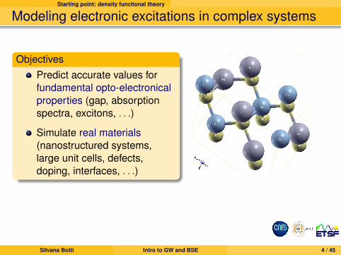
Modeling electronic excitations in complex systems
ObjectivesPredict accurate values forfundamental opto-electronicalproperties (gap, absorptionspectra, excitons, . . .)
Simulate real materials(nanostructured systems,large unit cells, defects,doping, interfaces, . . .)
Silvana Botti Intro to GW and BSE 4 / 45
Starting point: density functional theory
How do we study electronic excitations?
In a quantum-mechanical framework that describes, fromfirst-principles, a system of interacting electrons and nuclei in presenceof time-dependent external fieldsMany different possible ways:
Wave-function based: Hartree-Fock and Post-Hartree-Fockmethods, Monte Carlo, . . .Green’s function based: Many-body Perturbation Theory (GW,BSE)Density based: TDDFT
In order to study complex systems it is important to find a compromisebetween accuracy of results and computational effort
Silvana Botti Intro to GW and BSE 5 / 45
Starting point: density functional theory
The heart of density functional theory (DFT)
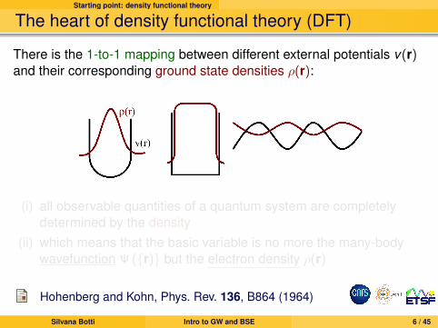
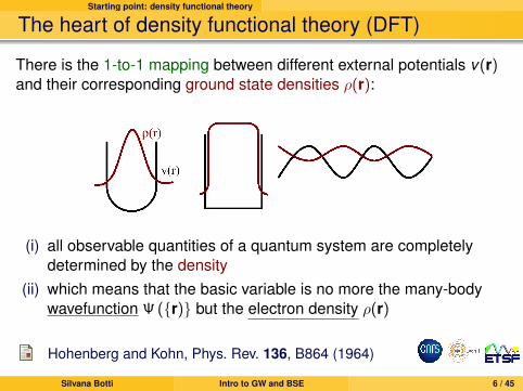
There is the 1-to-1 mapping between different external potentials v(r)and their corresponding ground state densities ρ(r):
(i) all observable quantities of a quantum system are completelydetermined by the density
(ii) which means that the basic variable is no more the many-bodywavefunction Ψ (r) but the electron density ρ(r)
Hohenberg and Kohn, Phys. Rev. 136, B864 (1964)
Silvana Botti Intro to GW and BSE 6 / 45
Starting point: density functional theory
The heart of density functional theory (DFT)
There is the 1-to-1 mapping between different external potentials v(r)and their corresponding ground state densities ρ(r):
(i) all observable quantities of a quantum system are completelydetermined by the density
(ii) which means that the basic variable is no more the many-bodywavefunction Ψ (r) but the electron density ρ(r)
Hohenberg and Kohn, Phys. Rev. 136, B864 (1964)
Silvana Botti Intro to GW and BSE 6 / 45
Starting point: density functional theory
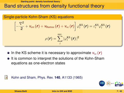
Band structures from density functional theory
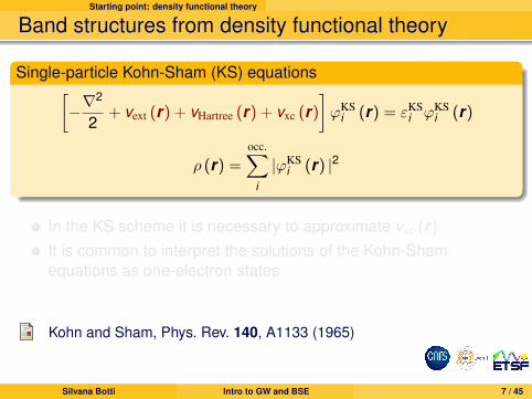
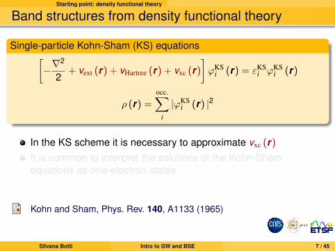
Single-particle Kohn-Sham (KS) equations[−∇
2
2+ vext (r) + vHartree (r) + vxc (r)
]ϕKS
i (r) = εKSi ϕKS
i (r)
ρ (r) =occ.∑
i
|ϕKSi (r) |2
In the KS scheme it is necessary to approximate vxc (r)
It is common to interpret the solutions of the Kohn-Shamequations as one-electron states
Kohn and Sham, Phys. Rev. 140, A1133 (1965)
Silvana Botti Intro to GW and BSE 7 / 45
Starting point: density functional theory
Band structures from density functional theory
Single-particle Kohn-Sham (KS) equations[−∇
2
2+ vext (r) + vHartree (r) + vxc (r)
]ϕKS
i (r) = εKSi ϕKS
i (r)
ρ (r) =occ.∑
i
|ϕKSi (r) |2
In the KS scheme it is necessary to approximate vxc (r)
It is common to interpret the solutions of the Kohn-Shamequations as one-electron states
Kohn and Sham, Phys. Rev. 140, A1133 (1965)
Silvana Botti Intro to GW and BSE 7 / 45
Starting point: density functional theory
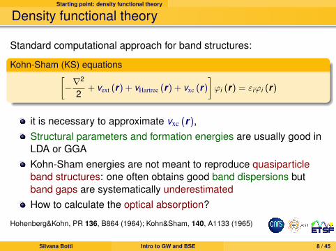
Density functional theory
Standard computational approach for band structures:
Kohn-Sham (KS) equations[−∇
2
2+ vext (r) + vHartree (r) + vxc (r)
]ϕi (r) = εiϕi (r)
it is necessary to approximate vxc (r),Structural parameters and formation energies are usually good inLDA or GGAKohn-Sham energies are not meant to reproduce quasiparticleband structures: one often obtains good band dispersions butband gaps are systematically underestimatedHow to calculate the optical absorption?
Hohenberg&Kohn, PR 136, B864 (1964); Kohn&Sham, 140, A1133 (1965)
Silvana Botti Intro to GW and BSE 8 / 45
Starting point: density functional theory
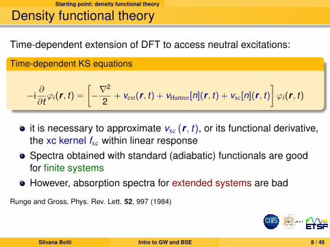
Density functional theory
Time-dependent extension of DFT to access neutral excitations:
Time-dependent KS equations
−i∂
∂tϕi (r , t) =
[−∇
2
2+ vext(r , t) + vHartree[n](r , t) + vxc[n](r , t)
]ϕi (r , t)
it is necessary to approximate vxc (r , t), or its functional derivative,the xc kernel fxc within linear responseSpectra obtained with standard (adiabatic) functionals are goodfor finite systemsHowever, absorption spectra for extended systems are bad
Runge and Gross, Phys. Rev. Lett. 52, 997 (1984)
Silvana Botti Intro to GW and BSE 8 / 45
Photoemission and optical absorption
Outline
1 Starting point: density functional theory
2 Photoemission and optical absorption
3 Beyond ground-state density functional theory
4 Green’s functions and GW approximation
5 Bethe-Salpeter equation and excitons
6 Summary
Silvana Botti Intro to GW and BSE 9 / 45
Photoemission and optical absorption
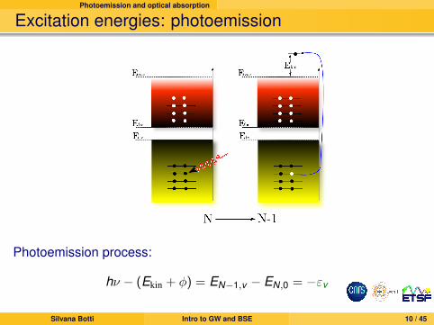
Excitation energies: photoemission
Photoemission process:
hν − (Ekin + φ) = EN−1,v − EN,0 = −εv
Silvana Botti Intro to GW and BSE 10 / 45
Photoemission and optical absorption
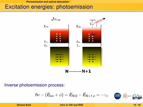
Excitation energies: photoemission
Inverse photoemission process:
hν − (Ekin + φ) = EN,0 − EN+1,c = −εc
Silvana Botti Intro to GW and BSE 10 / 45
Photoemission and optical absorption
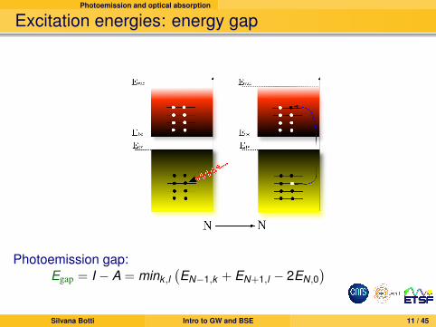
Excitation energies: energy gap
Photoemission gap:Egap = I − A = mink ,l
(EN−1,k + EN+1,l − 2EN,0
)Silvana Botti Intro to GW and BSE 11 / 45
Photoemission and optical absorption
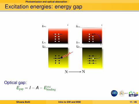
Excitation energies: energy gap
Optical gap:Egap = I − A− Eexc
binding
Silvana Botti Intro to GW and BSE 11 / 45
Photoemission and optical absorption
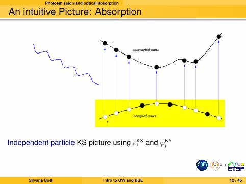
An intuitive Picture: Absorption
v
c
unoccupied states
occupied states
Independent particle KS picture using εKSi and ϕKS
i
Silvana Botti Intro to GW and BSE 12 / 45
Photoemission and optical absorption
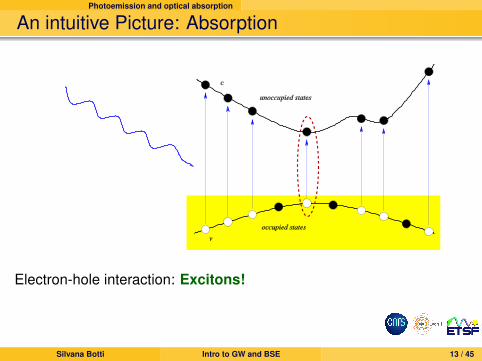
An intuitive Picture: Absorption
v
c
unoccupied states
occupied states
Electron-hole interaction: Excitons!
Silvana Botti Intro to GW and BSE 13 / 45
Photoemission and optical absorption
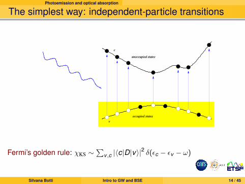
The simplest way: independent-particle transitions
v
c
unoccupied states
occupied states
Fermi’s golden rule: χKS ∼∑
v ,c |〈c|D|v〉|2 δ(εc − εv − ω)
Silvana Botti Intro to GW and BSE 14 / 45
Photoemission and optical absorption
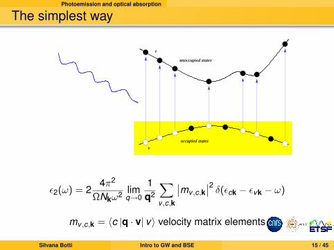
The simplest way
v
c
unoccupied states
occupied states
ε2(ω) = 24π2
ΩNkω2 limq→0
1q2
∑v ,c,k
∣∣mv ,c,k∣∣2 δ(εck − εvk − ω)
mv ,c,k = 〈c |q · v| v〉 velocity matrix elements
Silvana Botti Intro to GW and BSE 15 / 45
Photoemission and optical absorption
Joint density of states
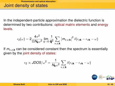
In the independent-particle approximation the dielectric function isdetermined by two contributions: optical matrix elements and energylevels.
ε2(ω) = 24π2
ΩNkω2 limq→0
1q2
∑v ,c,k
∣∣mv ,c,k∣∣2 δ(εck − εvk − ω)
If mv ,c,k can be considered constant then the spectrum is essentiallygiven by the joint density of states:
ε2 ∝ JDOS/ω2 =1
Nkω2
∑v ,c,k
δ(εck − εvk − ω)
Silvana Botti Intro to GW and BSE 16 / 45
Beyond ground-state density functional theory
Outline
1 Starting point: density functional theory
2 Photoemission and optical absorption
3 Beyond ground-state density functional theory
4 Green’s functions and GW approximation
5 Bethe-Salpeter equation and excitons
6 Summary
Silvana Botti Intro to GW and BSE 17 / 45
Beyond ground-state density functional theory
Time-dependent DFT for neutral excitations
Runge-Gross theoremThere is a one-to-one correspondence between the time-dependentdensity and the external potential, ρ(r , t)↔ v(r , t)
The many-body equation is mapped onto the time-dependentKohn-Sham equation:
−i∂
∂tφi(r , t) =
[−∇
2
2+ vext(r , t) + vHartree[n](r , t) + vxc[n](r , t)
]φi(r , t)
it is necessary to approximate vxc (r , t), or its functional derivative,the xc kernel fxc within linear response
Runge and Gross, Phys. Rev. Lett. 52, 997 (1984)
Silvana Botti Intro to GW and BSE 18 / 45
Beyond ground-state density functional theory
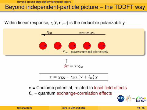
Beyond independent-particle picture – the TDDFT way
Within linear response, χ(r, r′, ω) is the reducible polarizability
V
Vind
ext
macroscopic and microscopic
macroscopic
↑δn = χvext
χ = χKS + χKS (v + fxc)χ
v = Coulomb potential, related to local field effectsfxc = quantum exchange-correlation effects
Silvana Botti Intro to GW and BSE 19 / 45
Beyond ground-state density functional theory
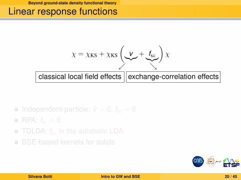
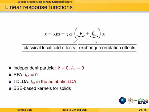
Linear response functions
χ = χKS + χKS
(v︸︷︷︸+ fxc︸︷︷︸
)χ
classical local field effects exchange-correlation effects
Independent-particle: v = 0, fxc = 0RPA: fxc = 0TDLDA: fxc in the adiabatic LDABSE-based kernels for solids
Silvana Botti Intro to GW and BSE 20 / 45
Beyond ground-state density functional theory
Linear response functions
χ = χKS + χKS
(v︸︷︷︸+ fxc︸︷︷︸
)χ
classical local field effects exchange-correlation effects
Independent-particle: v = 0, fxc = 0RPA: fxc = 0TDLDA: fxc in the adiabatic LDABSE-based kernels for solids
Silvana Botti Intro to GW and BSE 20 / 45
Green’s functions and GW approximation
Outline
1 Starting point: density functional theory
2 Photoemission and optical absorption
3 Beyond ground-state density functional theory
4 Green’s functions and GW approximation
5 Bethe-Salpeter equation and excitons
6 Summary
Silvana Botti Intro to GW and BSE 21 / 45
Green’s functions and GW approximation
A more “intuitive” path: electrons and holes
! "
! "#!
#" $" "" "!" "" "!
" "" "" " #
! "# " ! " " " " " "
#$" "" " #
! "# " ! " " " ! " "
#!" "" " #
! "%# ! "$ " " !" !" ! "
#!
!
Π0
!
! "&# $ " $ #
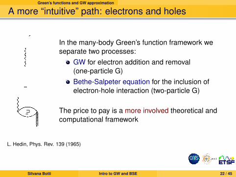
In the many-body Green’s function framework weseparate two processes:
GW for electron addition and removal(one-particle G)Bethe-Salpeter equation for the inclusion ofelectron-hole interaction (two-particle G)
The price to pay is a more involved theoretical andcomputational framework
L. Hedin, Phys. Rev. 139 (1965)
Silvana Botti Intro to GW and BSE 22 / 45
Green’s functions and GW approximation
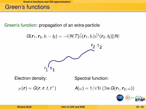
Green’s functions
Green’s function: propagation of an extra-particle
G(r1, r2, t1 − t2) = −i〈N|T [ψ(r1, t1)ψ†(r2, t2)]|N〉
Electron density:
ρ (r) = G(r , r , t , t+)
Spectral function:
A(ω) = 1/πTr Im G(r1, r2, ω)
Silvana Botti Intro to GW and BSE 23 / 45
Green’s functions and GW approximation
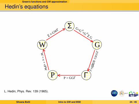
Hedin’s equations
Σ
G
ΓP
W
G=G 0+G 0 Σ G
Γ=1+
(δΣ/
δG)G
GΓ
P = GGΓ
W = v + vPW
Σ = GWΓ
L. Hedin, Phys. Rev. 139 (1965).
Silvana Botti Intro to GW and BSE 24 / 45
Green’s functions and GW approximation
Self-energy and screened interaction
Self-energy: nonlocal, non-Hermitian, frequency dependent operatorIt allows to obtain the Green’s function G once that G0 is known
Hartree-Fock Σx (r1, r2) = iG(r1, r2, t , t+)v(r1, r2)
GW Σ(r1, r2, t1 − t2) = iG(r1, r2, t1 − t2)W (r1, r2, t2 − t1)
W = ε−1v : screened potential (much weaker than v !)
Ingredients:KS Green’s function G0, and RPA dielectric matrix ε−1
G,G′(q, ω)
L. Hedin, Phys. Rev. 139 (1965)
Silvana Botti Intro to GW and BSE 25 / 45
Green’s functions and GW approximation
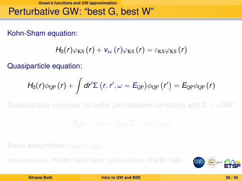
Perturbative GW: “best G, best W”
Kohn-Sham equation:
H0(r)ϕKS (r) + vxc (r)ϕKS (r) = εKSϕKS (r)
Quasiparticle equation:
H0(r)φQP (r) +
∫dr ′Σ
(r , r ′, ω = EQP
)φQP
(r ′)
= EQPφQP (r)
Quasiparticle energies 1st order perturbative correction with Σ = iGW :
EQP − εKS = 〈ϕKS|Σ− vxc|ϕKS〉
Basic assumption: φQP ' ϕKS
Hybersten&Louie, PRB 34 (1986); Godby, Schluter&Sham, PRB 37 (1988)
Silvana Botti Intro to GW and BSE 26 / 45
Green’s functions and GW approximation
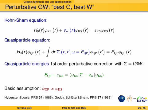
Perturbative GW: “best G, best W”
Kohn-Sham equation:
H0(r)ϕKS (r) + vxc (r)ϕKS (r) = εKSϕKS (r)
Quasiparticle equation:
H0(r)φQP (r) +
∫dr ′Σ
(r , r ′, ω = EQP
)φQP
(r ′)
= EQPφQP (r)
Quasiparticle energies 1st order perturbative correction with Σ = iGW :
EQP − εKS = 〈ϕKS|Σ− vxc|ϕKS〉
Basic assumption: φQP ' ϕKS
Hybersten&Louie, PRB 34 (1986); Godby, Schluter&Sham, PRB 37 (1988)
Silvana Botti Intro to GW and BSE 26 / 45
Green’s functions and GW approximation
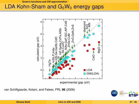
LDA Kohn-Sham and G0W0 energy gaps
0
2
4
6
8
calc
ula
ted g
ap (
eV
)
:LDA
:GW(LDA)
HgT
e
InS
b,P
,InA
sIn
N,G
e,G
aS
b,C
dO
Si
InP
,GaA
s,C
dT
e,A
lSb
Se,C
u2O
AlA
s,G
aP
,SiC
,AlP
,CdS
ZnS
e,C
uB
r
ZnO
,GaN
,ZnS
dia
mond
SrO A
lN
MgO
CaO
van Schilfgaarde, Kotani, and Faleev, PRL 96 (2006)
Silvana Botti Intro to GW and BSE 27 / 45
experimental gap (eV)
Green’s functions and GW approximation
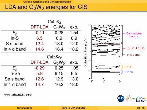
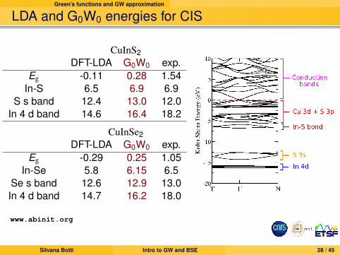
LDA and G0W0 energies for CIS
CuInS2DFT-LDA G0W0 exp.
Eg -0.11 0.28 1.54In-S 6.5 6.9 6.9
S s band 12.4 13.0 12.0In 4 d band 14.6 16.4 18.2
CuInSe2DFT-LDA G0W0 exp.
Eg -0.29 0.25 1.05In-Se 5.8 6.15 6.5
Se s band 12.6 12.9 13.0In 4 d band 14.7 16.2 18.0
www.abinit.org
Silvana Botti Intro to GW and BSE 28 / 45
Green’s functions and GW approximation
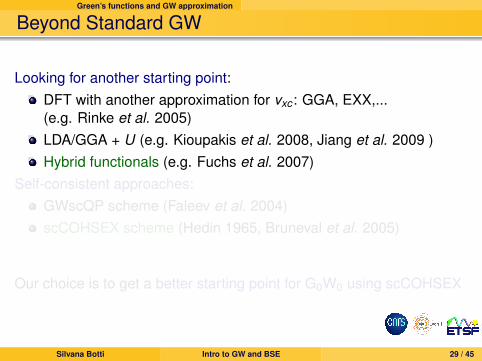
Beyond Standard GW
Looking for another starting point:DFT with another approximation for vxc : GGA, EXX,...(e.g. Rinke et al. 2005)LDA/GGA + U (e.g. Kioupakis et al. 2008, Jiang et al. 2009 )Hybrid functionals (e.g. Fuchs et al. 2007)
Self-consistent approaches:GWscQP scheme (Faleev et al. 2004)scCOHSEX scheme (Hedin 1965, Bruneval et al. 2005)
Our choice is to get a better starting point for G0W0 using scCOHSEX
Silvana Botti Intro to GW and BSE 29 / 45
Green’s functions and GW approximation
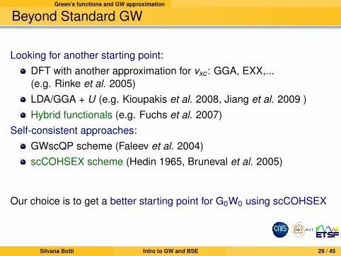
Beyond Standard GW
Looking for another starting point:DFT with another approximation for vxc : GGA, EXX,...(e.g. Rinke et al. 2005)LDA/GGA + U (e.g. Kioupakis et al. 2008, Jiang et al. 2009 )Hybrid functionals (e.g. Fuchs et al. 2007)
Self-consistent approaches:GWscQP scheme (Faleev et al. 2004)scCOHSEX scheme (Hedin 1965, Bruneval et al. 2005)
Our choice is to get a better starting point for G0W0 using scCOHSEX
Silvana Botti Intro to GW and BSE 29 / 45
Green’s functions and GW approximation
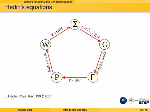
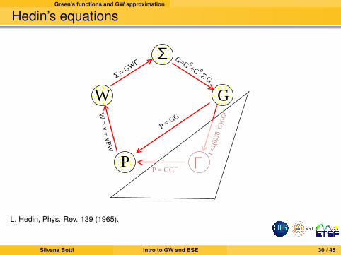
Hedin’s equations
Σ
G
ΓP
W
G=G 0+G 0 Σ G
Γ=1+
(δΣ/
δG)G
GΓ
P = GGΓ
W = v + vPW
Σ = GWΓ
L. Hedin, Phys. Rev. 139 (1965).
Silvana Botti Intro to GW and BSE 30 / 45
Green’s functions and GW approximation
Hedin’s equations
Σ
G
ΓP
W
G=G 0+G 0 Σ G
Γ=1+
(δΣ/
δG)G
GΓ
P = GGΓ
W = v + vPW
Σ = GWΓ
P = GG
L. Hedin, Phys. Rev. 139 (1965).
Silvana Botti Intro to GW and BSE 30 / 45

Green’s functions and GW approximation
COHSEX: approximation to GW self-energy
Coulomb hole:
ΣCOH(r1, r2) =12δ(r1 − r2)[W (r1, r2, ω = 0)− v(r1, r2)]
Screened Exchange:
ΣSEX(r1, r2) = −∑
i
θ(µ− Ei)φi(r1)φ∗i (r2)W (r1, r2, ω = 0)
The COHSEX self-energy is static and HermitianSelf-consistency can be done either on energies alone or on bothenergies and wavefunctionsRepresentation of WFs on a restricted LDA basis set
Silvana Botti Intro to GW and BSE 31 / 45
Green’s functions and GW approximation
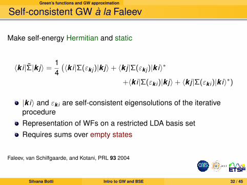
Self-consistent GW a la Faleev
Make self-energy Hermitian and static
〈k i |Σ|k j〉 =14(〈k i |Σ(εk j)|k j〉+ 〈k j |Σ(εk j)|k i〉∗
+〈k i |Σ(εk i)|k j〉+ 〈k j |Σ(εk i)|k i〉∗)
|k i〉 and εk i are self-consistent eigensolutions of the iterativeprocedureRepresentation of WFs on a restricted LDA basis setRequires sums over empty states
Faleev, van Schilfgaarde, and Kotani, PRL 93 2004
Silvana Botti Intro to GW and BSE 32 / 45
Green’s functions and GW approximation
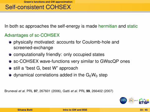
Self-consistent COHSEX
In both sc approaches the self-energy is made hermitian and static
Advantages of sc-COHSEXphysically motivated: accounts for Coulomb-hole andscreened-exchangecomputationally friendly: only occupied statessc-COHSEX wave-functions very similar to GWscQP onesstill a “best G, best W” approachdynamical correlations added in the G0W0 step
Bruneval et al. PRL 97, 267601 (2006), Gatti et al. PRL 99, 266402 (2007)
Silvana Botti Intro to GW and BSE 33 / 45
Green’s functions and GW approximation
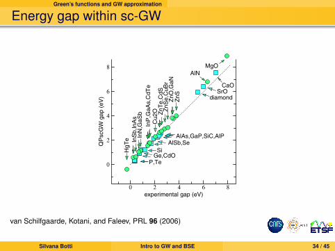
Energy gap within sc-GW
0 2 4 6 8
0
2
4
6
8
experimental gap (eV)
QP
scG
W g
ap
(e
V)
MgO
AlN
CaO
HgT
e InS
b,I
nA
sIn
N,G
aS
b
InP
,Ga
As,C
dT
eC
u2
O Zn
Te
,Cd
SZ
nS
e,C
uB
rZ
nO
,Ga
NZ
nS
P,Te
SiGe,CdO
AlSb,SeAlAs,GaP,SiC,AlP
SrOdiamond
van Schilfgaarde, Kotani, and Faleev, PRL 96 (2006)
Silvana Botti Intro to GW and BSE 34 / 45
Green’s functions and GW approximation
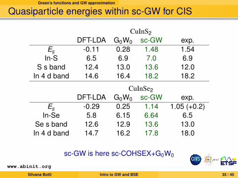
Quasiparticle energies within sc-GW for CIS
CuInS2DFT-LDA G0W0 sc-GW exp.
Eg -0.11 0.28 1.48 1.54In-S 6.5 6.9 7.0 6.9
S s band 12.4 13.0 13.6 12.0In 4 d band 14.6 16.4 18.2 18.2
CuInSe2DFT-LDA G0W0 sc-GW exp.
Eg -0.29 0.25 1.14 1.05 (+0.2)In-Se 5.8 6.15 6.64 6.5
Se s band 12.6 12.9 13.6 13.0In 4 d band 14.7 16.2 17.8 18.0
sc-GW is here sc-COHSEX+G0W0
www.abinit.org
Silvana Botti Intro to GW and BSE 35 / 45
Bethe-Salpeter equation and excitons
Outline
1 Starting point: density functional theory
2 Photoemission and optical absorption
3 Beyond ground-state density functional theory
4 Green’s functions and GW approximation
5 Bethe-Salpeter equation and excitons
6 Summary
Silvana Botti Intro to GW and BSE 36 / 45
Bethe-Salpeter equation and excitons
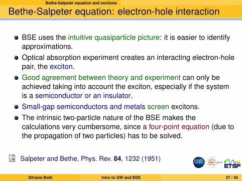
Bethe-Salpeter equation: electron-hole interaction
BSE uses the intuitive quasiparticle picture: it is easier to identifyapproximations.Optical absorption experiment creates an interacting electron-holepair, the exciton.Good agreement between theory and experiment can only beachieved taking into account the exciton, especially if the systemis a semiconductor or an insulator.Small-gap semiconductors and metals screen excitons.The intrinsic two-particle nature of the BSE makes thecalculations very cumbersome, since a four-point equation (due tothe propagation of two particles) has to be solved.
Salpeter and Bethe, Phys. Rev. 84, 1232 (1951)
Silvana Botti Intro to GW and BSE 37 / 45
Bethe-Salpeter equation and excitons
Bethe-Salpeter equation: electron-hole interaction
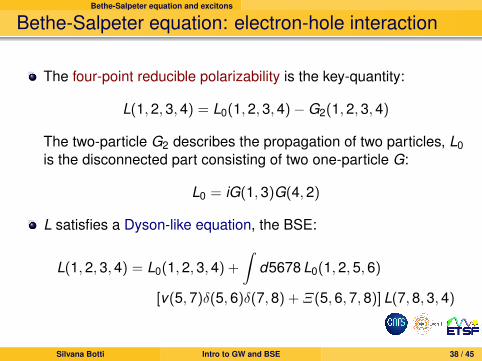
The four-point reducible polarizability is the key-quantity:
L(1,2,3,4) = L0(1,2,3,4)−G2(1,2,3,4)
The two-particle G2 describes the propagation of two particles, L0is the disconnected part consisting of two one-particle G:
L0 = iG(1,3)G(4,2)
L satisfies a Dyson-like equation, the BSE:
L(1,2,3,4) = L0(1,2,3,4) +
∫d5678 L0(1,2,5,6)
[v(5,7)δ(5,6)δ(7,8) +Ξ(5,6,7,8)] L(7,8,3,4)
Silvana Botti Intro to GW and BSE 38 / 45
Bethe-Salpeter equation and excitons
Bethe-Salpeter equation: electron-hole interaction
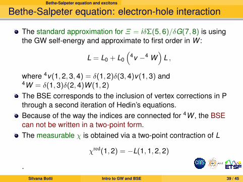
The standard approximation for Ξ = iδΣ(5,6)/δG(7,8) is usingthe GW self-energy and approximate to first order in W :
L = L0 + L0
(4v −4 W
)L ,
where 4v(1,2,3,4) = δ(1,2)δ(3,4)v(1,3) and4W = δ(1,3)δ(2,4)W (1,2)
The BSE corresponds to the inclusion of vertex corrections in Pthrough a second iteration of Hedin’s equations.Because of the way the indices are connected for 4W , the BSEcan not be written in a two-point form.The measurable χ is obtained via a two-point contraction of L
χred(1,2) = −L(1,1,2,2)
.Silvana Botti Intro to GW and BSE 39 / 45
Bethe-Salpeter equation and excitons
Bethe-Salpeter equation: electron-hole interaction
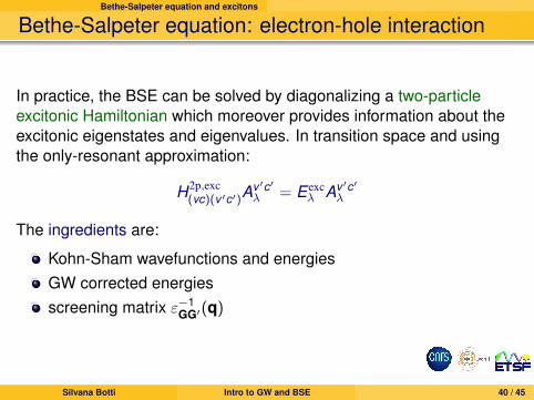
In practice, the BSE can be solved by diagonalizing a two-particleexcitonic Hamiltonian which moreover provides information about theexcitonic eigenstates and eigenvalues. In transition space and usingthe only-resonant approximation:
H2p,exc(vc)(v ′c′)A
v ′c′
λ = Eexcλ Av ′c′
λ
The ingredients are:
Kohn-Sham wavefunctions and energiesGW corrected energiesscreening matrix ε−1
GG′(q)
Silvana Botti Intro to GW and BSE 40 / 45
Bethe-Salpeter equation and excitons
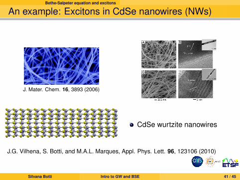
An example: Excitons in CdSe nanowires (NWs)
J. Mater. Chem. 16, 3893 (2006)
CdSe wurtzite nanowires
J.G. Vilhena, S. Botti, and M.A.L. Marques, Appl. Phys. Lett. 96, 123106 (2010)
Silvana Botti Intro to GW and BSE 41 / 45
Bethe-Salpeter equation and excitons
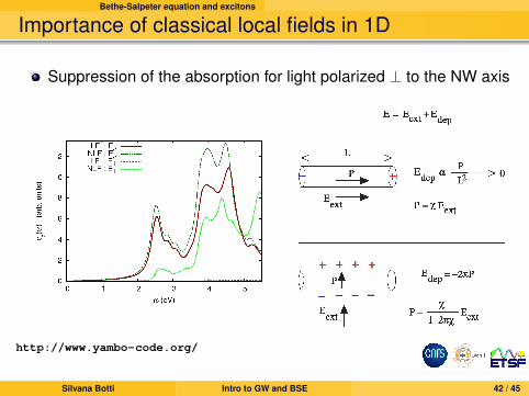
Importance of classical local fields in 1D
Suppression of the absorption for light polarized ⊥ to the NW axis
http://www.yambo-code.org/
Silvana Botti Intro to GW and BSE 42 / 45
Bethe-Salpeter equation and excitons
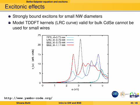
Excitonic effects
Strongly bound excitons for small NW diametersModel TDDFT kernels (LRC curve) valid for bulk CdSe cannot beused for small wires
http://www.yambo-code.org/
Silvana Botti Intro to GW and BSE 43 / 45
Summary
Outline
1 Starting point: density functional theory
2 Photoemission and optical absorption
3 Beyond ground-state density functional theory
4 Green’s functions and GW approximation
5 Bethe-Salpeter equation and excitons
6 Summary
Silvana Botti Intro to GW and BSE 44 / 45
Summary
Summary
Methods that go beyond ground-state DFT are by now well established
However one should remember that interpretation of experiments isoften not straightforwardA better starting point is absolutely necessary for d-electrons
Self-consistent COHSEX+G0W0 gives a very good description ofquasi-particle statesHybrid functionals can be a good compromiseLDA+U can not work when there is hybridization of p − d states
For accurate absorpion spectra when excitonic effects are importantone has to solve the Bethe-Salpeter equation.
Silvana Botti Intro to GW and BSE 45 / 45


![On the relativistic field-theoretical three dimensional ... · The modern three-body formulation of the Bethe-Salpeter equations was given in [13,14]. This formulation was performed](https://img.pdfslide.us/doc/110x75/5f31806dab170c1c3f6515ff/on-the-relativistic-field-theoretical-three-dimensional-the-modern-three-body.jpg)