Introduction to Graph Mining

What is a graph?

• A graph G = (V,E) is a set of vertices V and a set (possibly empty) E of

pairs of vertices e1 = (v

1, v

2), where e

1 E and v

1, v

2 V.

• Edges may

• contain weights

• contain labels

• have direction

• Nodes may

• contain additional labels

• Formal study of graphs is called graph theory.

Motivation

• Many domains produce data that can be intuitively

represented by graphs.

• We would like to discover interesting facts and information

about these graphs.

• Real world graph datasets too large for humans to make any

sense of.

• We would like to discover patterns that have structural

information present.

Application Domains

• Web structure graphs

• Social networks

• Protein interaction networks

• Chemical compound

• Program Flow

• Transportation networks

Graph Mining Problems

• Graph Theoretic Problems

• Radius

• Diameter

• Graph Statistics:

• Degree Distribution

• Clustering Co-efficient

• Data Mining Problems

• Pattern Mining

• Clustering

• Classification / Prediction

• Compression

• Modelling

Researchers

• Xifeng Yan – UC Santa Barbara

• Jiawei Han - U Illinois Urbana Champaign

• George Karypis – U Minnesota

• Charu Aggarwal – IBM T.J. Watson Research Center

• Jennifer Neville – Purdue University

Social Network Analysis

with graphs!

del.icio.us visualization by Kunal Anand

Social Network Analysis

• Interested in populations not individuals

• Structure within society

Social Network Analysis

•Network (Graph)

• Nodes: Things (people, places, etc.)

• Edges: Relationships (friends, visited, etc.)

Quantitative Analysis

•Analysis

• Quantitative not qualitative

• Usually Scale-Free Networks

Further Resources

• Social network analysis: methods and

applications

–Stanley Wasserman & Katherine Faust

•Christos Faloutsos, Watch the video

• Jure Leskovec @ Stanford

• The Mining Graph Data book

Towards Proximity Pattern Mining in Large Graphs

Arijit Khan, Xifeng Yan, Kun-Lung Wu

Overview

• Detects novel type of pattern in large graphs called proximity

patterns

• Develop two models to model the growth of proximity patterns

• Use a probabilistic frequent pattern miner to extract proximity

patterns

• Test their approach on Last.fm, Intrusion Alert Network, DBLP

Collaboration Graph. Evaluate the interestingness of patterns

generated using a statistical measure.

What is a proximity pattern?

• “A proximity pattern is a subset of labels that repeatedly appear in

multiple tightly connected subgraphs” – (from [1]).

• Characteristics of proximity patterns:

• Labels in pattern are tightly connected

• They are frequent

• They may not be connected in the same way always

• Useful in modelling information flow in a dynamic graph

Proximity

Pattern: {a,b,c}

Definitions

• The support sup(I) of an itemset P⊆ L (the set of labels) is the

number of transactions in the data set that I is present in.

• A frequent itemset is an itemset which has a support greater

than an user-defined threshold.

• The downward closure property of an itemset states that all

subsets of a frequent itemset are frequent. Consequently all

supersets of an infrequent itemset are infrequent.

Definitions

• Given a graph G = (V,E) and a subset of vertices π, π ∈ V (G), let

L(π) be the set of labels in π, i.e., L(π) = ∪u ∈ π

L(u). Given a label

subset I, π is called an embedding of I if I ⊆ L(π). The vertices in

π need not be connected. (from [1])

• A mapping φ between I and the vertices in π is a function φ:I →

π s.t., ∃ l, φ(l) ∈ π and l ∈ L(φ(l)). A mapping is minimum if it is

surjective, i.e., ∀v ∈ π, ∃l s.t. φ(l) = v. (from [1])

• Given an itemset I and a mapping φ, we need a function f(φ) to

measure its association strength. (from [1])

•{v1,v2,v3} is an embedding of {l1,l2,l5}

•Φ1(l1,l2,l5) = (v2,v1,v3) (minimum)

•Φ2(l1,l2,l5) = (v2,v3,v3) (non-minimum)

Neighbour Association Model

• Procedure:

• Find all embeddings π1,

π2, …,

πm of an itemset I.

• For each embedding π measure the strength f(π)

• Support of itemset I = ∑i=1

m f(π).

• Problems are:

• Support count based on overlapping embeddings violate the

downward closure property

• Any subset of vertices could be an embedding.

• To solve the first problem, a overlap graph is created. The

support is the sum of weights of the nodes in the maximum

weight independent set of this graph.

• Disadvantages:

• NP-Hard w.r.t. to the number of embeddings for a given pattern.

• Not feasible to generate all the embeddings for a pattern as there

could be a large number of embeddings

• Support count is NP-Complete.

Information Propagation Model

• G0 → G

1 → G

i →. . . → G

n

• Let L(u) be the present state of u, denoted by the labels present in

u, and l be a distinct label propagated by one of its neighbors and

l L(u). Hence, the probability of observing L(u) and l is written as:

P(L ∪ {l}) = P(L|l)P(l),

where P(l) is the probability of l in u‟s neighbors and P(L|l) is the

probability that l is successfully propagated to u.

• For multiple labels, l1, l

2, . . . , l

m,

P(L∪{l1, l

2, . . . , l

m}) = P(L|l

1)∗. . .∗ P(L|l

m)∗P(l

1)∗. . . P(l

m).

• Propagation model indicates the characteristic of social networks

where the influence of a given node on any other decreases as the

distance from the given node to the other node increases.

Nearest Probabilistic Association

• Au(l) = P(L(u)|l) = e

-.d,

where „l‟ is a label present in a vertex „v‟ closest to „u‟,

„d‟ is the distance from „v‟ to „u‟ (=1 for unweighted graph)

„‟ is the decay constant ( > 0)

• Probabilistic Support of I:

• If I = {l1, l2, . . . ,m} and J = {l1, l2, . . . , lm, lm+1 . . . , n}, then

since,

sup(I) sup(J)

Nearest Probabilistic Association

Nearest Probabilistic Association

Consistency between NPA and Frequent Itemset

Problem with NPA

NPA – Complexity, Advantages and

Disadvantages

• O(|V| . dt . s ),

• V is the total no. of vertices

• „d‟ is the average degree

• „t‟ is the number of iterations

• „s‟ is the number of labels in every vertex

• Advantage: It is fast to calculate

• Disadvantage: Considers only the nearest neighbour for

propagation.

Normalized Probabilistic Association

• Normalized Probabilistic Association of label „l‟ at vertex „u‟

• NMPA can break ties when

• two vertices have the same number of neighbors

• two vertices have different number of neighbours but the same

number of neighbours having label „l‟.

• The update rule of Algorithm 1 is changed:

• Complexity same as NPA, however propagation decays faster

due to normalization.

Probabilistic Itemset Mining

• Uses a probablistic version of FP-growth algorithm[3][4] to mine

frequent itemsets from uncertain data.

• Two variations of probabilistic FP-growth algorithm used

• Exact Mining: Using an FP-tree where nodes are augmented with the

probability values present in the proximity patterns

• Approximate Mining: FP-tree augmented not with all probability

values, but only sum of probability values and number of occurrences.

• C. Aggarwal et al. in [2] proposes various techniques to mine

frequent patterns from uncertain data. Probabilistic version of H-

Mine found to be the best.

Experiments

• Datasets used

• LAST.FM: Nodes labelled with artists, edges represent

communication between users

• Intrusion Alert Network: Node is a computer labelled with attacks,

edge represents possible attack

• DBLP Collaboration Graph: Nodes represent authors labelled with

keywords, edges represent collaboration.

• Labels are randomized and G-test score used to compare

between the support of patterns in actual graph and

randomized graph.

Experiments

• Effectiveness test:

Experiments

• Efficiency and Scalability

Experiments

• Exact vs. Approximate Mining

• Gives more proximity patterns than Frequent Subgraph Mining, and is

faster as it avoids isomorphism checking

Strengths

• Discovers new kind of patterns.

• Considers structure without incurring isomorphism checking.

• Applicable to weighted and un-weighted graphs.

• Can be extended to directed graphs

Weaknesses

• Run-time exponential with depth of propagation.

• Proximity pattern itself does not retain structural information.

• Large number of patterns might be generated.

• Different paths in the graph might have different decay rates.

Discussions

• What real life graphs/problems might this approach be really

good for?

• Is there a better way to determine proximity?

• What modifications would be needed for the technique to

handle directed subgraphs?

• How does the rate of decay affect the patterns found?

• How well will the approach fare when graphs have billions of

nodes and edges or more?

References

1. A. Khan, X. Yan, and K.-L.Wu. Towards proximity pattern

mining in large graphs. In SIGMOD, 2010.

2. C.C. Aggarwal, Y. Li, J. Wang, J. Wang. Frequent Pattern

Mining with Uncertain Data. KDD 2009.

3. Presentation on Frequent Pattern Growth (FP-Growth)

Algorithm: An Introduction by Florian Verhein

4. J. Han, J. Pei, Y. Yin. Mining frequent patterns without

candidate generation. SIGMOD, 2000.

What are your research

problems?

Avista Data (HW 4)

Radius Plots for Mining

Tera-byte Scale Graphs

Algorithms, Patterns, and

Observations

Authors

•U. Kang (CMU)

•C. Tsourakakis (CMU)

•A. Appel (USP São Carlos)

•C. Faloutsos (CMU)

• J. Leskovec (Stanford)

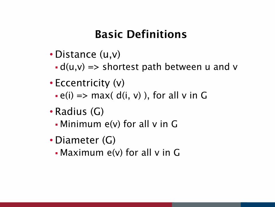
Basic Definitions

•Distance (u,v)

d(u,v) => shortest path between u and v

• Eccentricity (v)

e(i) => max( d(i, v) ), for all v in G

• Radius (G)

Minimum e(v) for all v in G

•Diameter (G)

Maximum e(v) for all v in G

Big Data

• YahooWeb

6B edges, 125GB on disk

–TBs of memory required to run algos

–Large enough nobody else has published on it

• Billion Triple Challenge

• ~2B edges

• Social networking data

• Spinn3r

•Google‟s 1T word language model

Flajolet-Martin

• Probabilistic counting paper from 1985

•Given

• M => K x 64 bit matrix

• h(a) => mostly uniform 64-bit hashing function

• ρ(a) => index of lowest cleared bit in a

• Pseudo-Code

• For x in data:

• M[ h(x) % K, ρ( h(x)/K ) ] = 1

• S=0

• For row in M:

• from i=0 until row[i++] == 0:

• S += i

• Return K/0.77351 * 2S/K

Flajolet-Martin for Radius Estimation

•Authors set K to 32

Original paper shows this gives stdev 13% error

• 64-bit bitstrings used

• Bit-Shuffle Encoding

Only pass around the number of starting 1s

and ending 0s

Optimizes network load

http://d3.do/en/?p=306

Map/Reduce in a nutshell

• From the paper:

MapReduce is a programming model and an associated

implementation for processing and generating large data

sets. Users specify a map function that processes a

key/value pair to generate a set of intermediate key/value

pairs, and a reduce function that merges all intermediate

values associated with the same intermediate key.

• Implementation is out of our scope

MapReduce/Hadoop Radius

•Map: Output (node_id, list of neighbor

bitstrings)

• Reduce: Add bitstrings to my own

•Optimizations

• Bundle edges into blocks

• Change bitstring to count blocks

• Perform sequence length encoding on

bitstrings

Recall Basic Definitions

•Distance (u,v)

d(u,v) => shortest path between u and v

• Eccentricity (v)

e(i) => max( d(i, v) ), for all v in G

• Radius (G)

Minimum e(v) for all v in G

•Diameter (G)

Maximum e(v) for all v in G

Visualizing HADI

Network Dynamics

•Why diameter shrinks over time

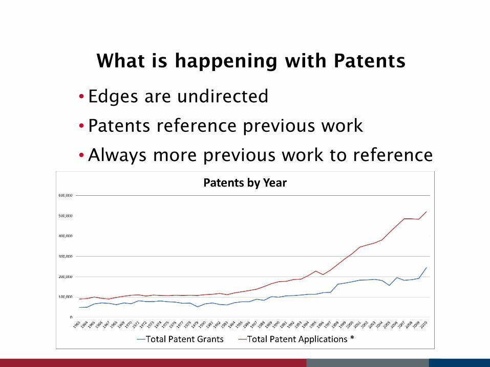
What is happening with Patents

• Edges are undirected

• Patents reference previous work

•Always more previous work to reference

Network Dynamics

• Patent vs. LinkedIn

• See HADI: Mining Radii of Large Graphs

Other observations

• “Surprising” diameter of 7~8

Could be a PageRank effect of SEO

Graph structure in the web

Broder et al., 2000

Discussion

•Can you represent your research problem as

a graph?

• Should you?

•Would it be useful to know how fast

information can propagate through your

graph?

•Can you breakdown your approach into a

map/reduce paradigm?

Graphs are pretty, look at them more!