IntroductiontoGPSmonitoringofdeformationatPu’u‘O’o,Hawaii

IntroductiontoGlobalPositioningSystems(GPS) The following text and images are taken from the USGS website: Volcano Exploration Program: Pu’u ‘O’o; URL: http://ulua.wr.usgs.gov/vepp

The use of the Global Positioning System (GPS) in Earth sciences has only been prominent since the 1980s, but since then has become nearly ubiquitous in volcano deformation measurements around the world. The system relies on a ground-based receiver and antenna, which records signals broadcast by an array of orbiting satellites. Given enough data, GPS data can be used to determine positions to within a few mm horizontally and ~10 mm vertically. GPS can be used in campaign mode, where a receiver and antenna are moved frequently to measure a series of fixed benchmarks (emblems permanently cemented into the ground) or installed for continuous measurement of surface motion at a single location. Typically, continuous GPS stations are powered by a combination of batteries and solar panels. The data received by continuous GPS stations are susceptible to a number of environmental effects unrelated to volcano deformation. For example, snow buildup on a GPS antenna can cause path delays, rain can induce surface loading, small movements can be detected due to diurnal or seasonal temperature variations, and most importantly, storms and other atmospheric phenomena can introduce deformation artifacts. Fortunately, atmospherically-based problems are less likely to affect tightly-clustered GPS networks, since all stations in such a network will see the same phenomena, and such effects will be canceled out.

GPSNetworkatPu‘u‘Ō‘ō

There are over 60 continuously operating GPS stations on the Island of Hawai‘i, most of which are operated by the Hawaiian Volcano Observatory for the purpose of earthquake and volcano monitoring. All stations have a GPS antenna mounted on a mast that is cemented into solid rock. The antenna is connected to a receiver which is typically run using a combination of solar and battery power. Data are collected at least every 30s and, at some stations, every 1s, and periodically

radioed to the Hawaiian Volcano Observatory where processing is completed and positions calculated.

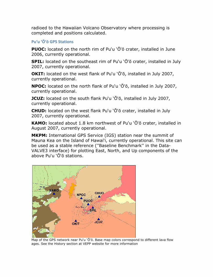
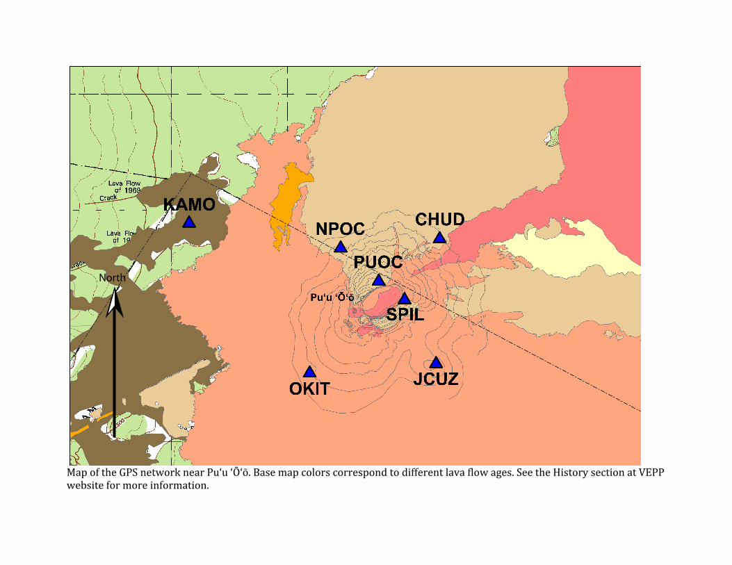
Pu‘u‘Ō‘ōGPSStations

PUOC: located on the north rim of Pu‘u ‘Ō‘ō crater, installed in June 2006, currently operational.

SPIL: located on the southeast rim of Pu‘u ‘Ō‘ō crater, installed in July 2007, currently operational.

OKIT: located on the west flank of Pu‘u ‘Ō‘ō, installed in July 2007, currently operational.

NPOC: located on the north flank of Pu‘u ‘Ō‘ō, installed in July 2007, currently operational.

JCUZ: located on the south flank Pu‘u ‘Ō‘ō, installed in July 2007, currently operational.

CHUD: located on the west flank Pu‘u ‘Ō‘ō crater, installed in July 2007, currently operational.

KAMO: located about 1.8 km northwest of Pu‘u ‘Ō‘ō crater, installed in August 2007, currently operational.

MKPM: International GPS Service (IGS) station near the summit of Mauna Kea on the Island of Hawai‘i, currently operational. This site can be used as a stable reference (''Baseline Benchmark'' in the Data-VALVE3 interface) for plotting East, North, and Up components of the above Pu‘u ‘Ō‘ō stations.

Map of the GPS network near Pu‘u ‘Ō‘ō. Base map colors correspond to different lava flow ages. See the History section at VEPP website for more information

Example:CGPSatKīlaueaVolcano,Hawai‘i

The use of GPS in volcano monitoring is exemplified by deformation during the June 17-19 intrusion and eruption near Makaopuhi Crater on Kīlauea's east rift zone (the so-called 'Father's Day event', also referred to as Episode 56 of the Pu‘u ‘Ō‘ō-Kupaianaha eruption).

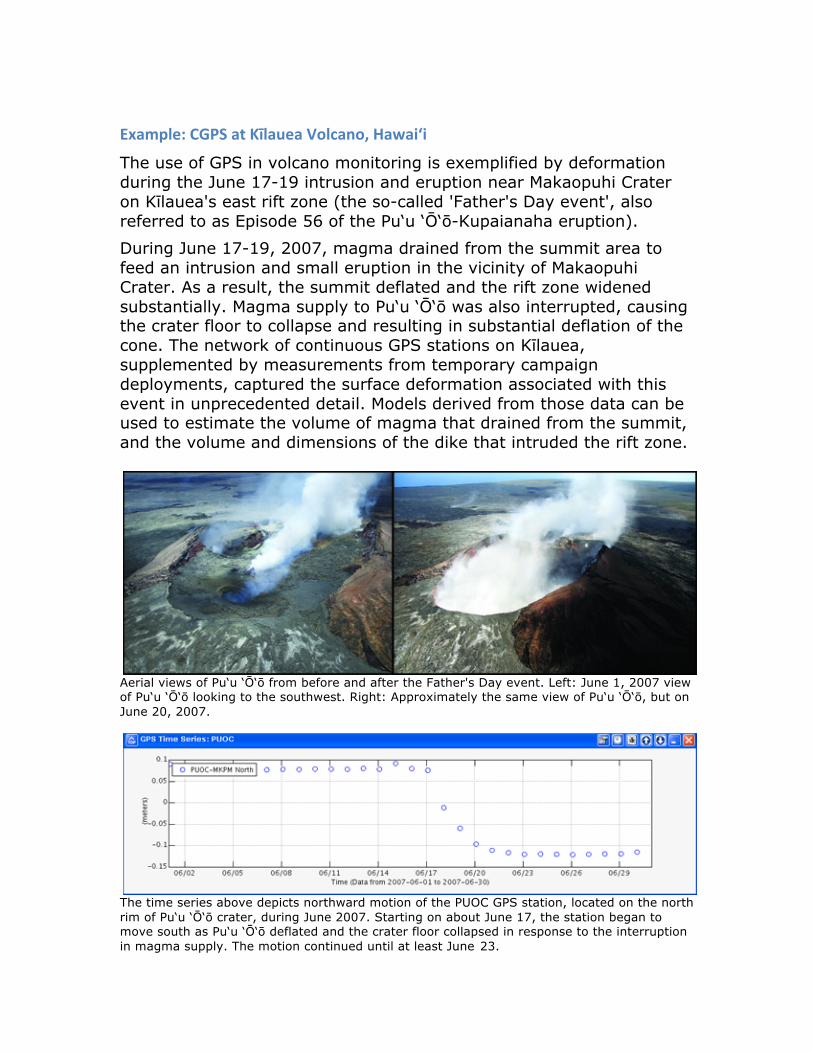
During June 17-19, 2007, magma drained from the summit area to feed an intrusion and small eruption in the vicinity of Makaopuhi Crater. As a result, the summit deflated and the rift zone widened substantially. Magma supply to Pu‘u ‘Ō‘ō was also interrupted, causing the crater floor to collapse and resulting in substantial deflation of the cone. The network of continuous GPS stations on Kīlauea, supplemented by measurements from temporary campaign deployments, captured the surface deformation associated with this event in unprecedented detail. Models derived from those data can be used to estimate the volume of magma that drained from the summit, and the volume and dimensions of the dike that intruded the rift zone.

Aerial views of Pu‘u ‘Ō‘ō from before and after the Father's Day event. Left: June 1, 2007 view of Pu‘u ‘Ō‘ō looking to the southwest. Right: Approximately the same view of Pu‘u ‘Ō‘ō, but on June 20, 2007.

The time series above depicts northward motion of the PUOC GPS station, located on the north rim of Pu‘u ‘Ō‘ō crater, during June 2007. Starting on about June 17, the station began to move south as Pu‘u ‘Ō‘ō deflated and the crater floor collapsed in response to the interruption in magma supply. The motion continued until at least June 23.

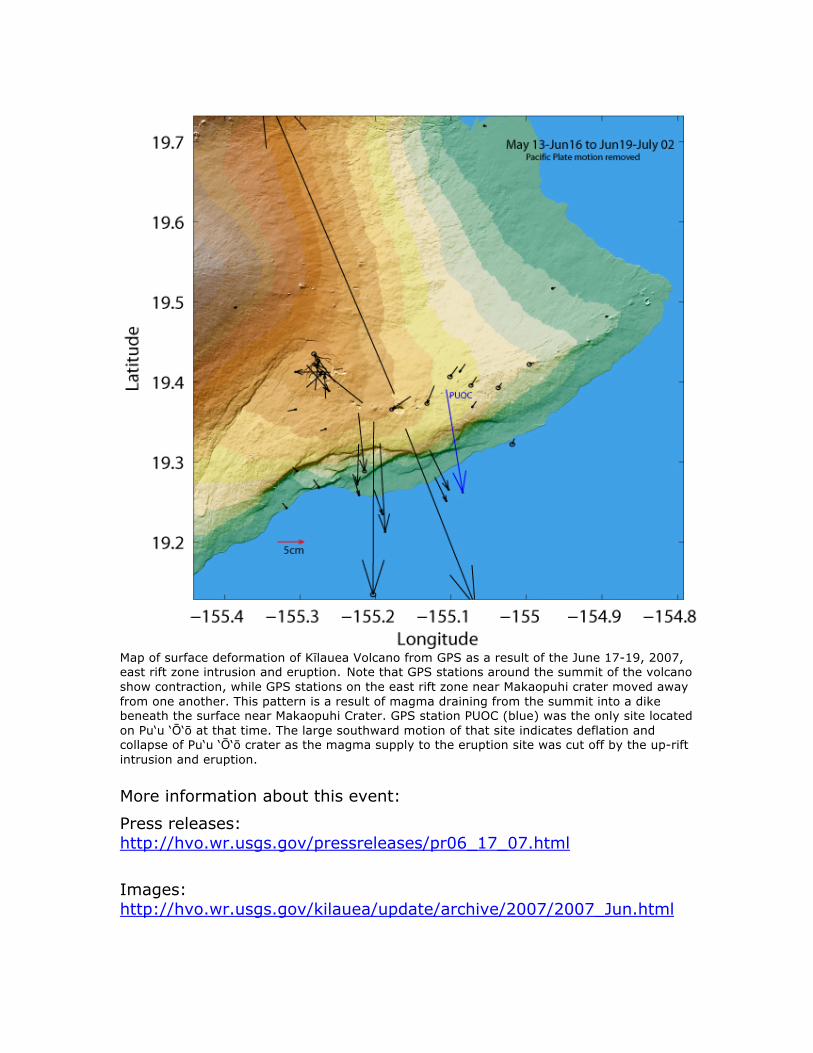
Map of surface deformation of Kīlauea Volcano from GPS as a result of the June 17-19, 2007, east rift zone intrusion and eruption. Note that GPS stations around the summit of the volcano show contraction, while GPS stations on the east rift zone near Makaopuhi crater moved away from one another. This pattern is a result of magma draining from the summit into a dike beneath the surface near Makaopuhi Crater. GPS station PUOC (blue) was the only site located on Pu‘u ‘Ō‘ō at that time. The large southward motion of that site indicates deflation and collapse of Pu‘u ‘Ō‘ō crater as the magma supply to the eruption site was cut off by the up-rift intrusion and eruption.

More information about this event:

Press releases: http://hvo.wr.usgs.gov/pressreleases/pr06_17_07.html

Images: http://hvo.wr.usgs.gov/kilauea/update/archive/2007/2007_Jun.html

References Cervelli, P., Segall, P., Amelung, F., Garbeil, H., Owen, S., Miklius, A., and Lisowski, M., 2002, The 12 September 1999 Upper east rift zone dike intrusion at Kīlauea Volcano, Hawai‘i: Journal of Geophysical Research, v. 107, no. B7, 2150, doi:10.1029/2001JB000602. Desmarais, E.K., and Segall, P., 2007, Transient deformation following the 30 January 1997 dike intrusion at Kīlauea volcano, Hawai‘i: Bulletin of Volcanology, v. 69, no. 4, p. 353-363. Miklius, A., Cervelli, P., Sako, M., Lisowski, M., Owen, S., Segall, P., Foster, J., Kamibayashi, K., and Brooks, B., 2005, Global Positioning System Measurements on the Island of Hawai‘i: 1997 through 2004: U.S. Geological Survey Open-File Report 2005-1425, 46 p. Montgomery-Brown, E.K., Sinnett, D.K., Poland, M.P., Segall, P., Orr, T., Zebker, H., and Miklius, A., in press, Geodetic evidence for en echelon dike emplacement and concurrent slow-slip at Kīlauea volcano, Hawai‘i, June 17, 2007: Journal of Geophysical Research. Owen, S., Segall, P., Freymueller, J.T., Miklius, A., Denlinger, R.P., Arnadottir, T., Sako, M.K., and Bürgmann, R., 1995, Rapid deformation of the south flank of Kīlauea Volcano, Hawai‘i: Science, v. 267, no. 5202, p. 1328-1332. Owen, S., Segall, P., Lisowski, M., Miklius, A., Denlinger, R., and Sako, M., 2000, Rapid deformation of Kīlauea Volcano: Global Positioning System measurements between 1990 and 1996: Journal of Geophysical Research, v. 105, no. B8, p. 18,983-18,993. Owen, S., Segall, P., Lisowski, M., Miklius, A., Murray, M., Bevis, M., and Foster, J., 2000, January 30, 1997 eruptive event on Kīlauea Volcano, Hawai‘i, as monitored by continuous GPS: Geophysical Research Letters, v. 27, no. 17, p. 2757-2760. Poland, M.P., Miklius, A., Orr, T., Sutton, A.J., Thornber, C.R., and Wilson, D., 2008, New episodes of volcanism at Kīlauea Volcano, Hawai‘i: EOS, Transactions, American Geophysical Union, v. 89, no. 5, p. 37-38. Segall, P., Cervelli, P., Owen, S., Lisowski, M., and Miklius, A., 2001, Constraints on dike propagation from continuous GPS measurements: Journal of Geophysical Research, v. 107, no. B9, p. 19,301-19,317.

IntroductiontobasicvectorsFrom Wikipedia: http://en.wikipedia.org/wiki/Euclidean_vector

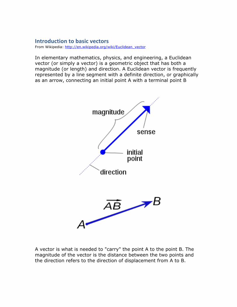
In elementary mathematics, physics, and engineering, a Euclidean vector (or simply a vector) is a geometric object that has both a magnitude (or length) and direction. A Euclidean vector is frequently represented by a line segment with a definite direction, or graphically as an arrow, connecting an initial point A with a terminal point B

A vector is what is needed to "carry" the point A to the point B. The magnitude of the vector is the distance between the two points and the direction refers to the direction of displacement from A to B.

IntroductiontoGPSmonitoringofdeformationatPu’u‘O’o,Hawaii

CLASSACTIVITY:

Materialsforactivity1. Background text about continuous GPS data with example from

Kilauea 2. Copy of Pu’u ‘O’o location map showing GPS sites around vent. 3. Time series for selected sites showing north, east and up

components of GPS motion over a select time period (3 are included here: SPIL, PUOC, JCUZ

4. Access to internet 5. Questions relating to analysis. 6. Colored pencils 7. Protractor 8. Ruler

Whattoturnin:1. Answers to questions 2. Table of observations and calculations 3. Annotated time series 4. Three vector graphs as described in exercise

Preparation

Collect the materials listed above to be ready to complete this exercise.

Read the provided information about GPS data andvectors. Refer to these information sheets as needed in this project.

As part of your background reading, refer to the USGS-VEPP website (password protected) to read about the history of Pu’u ‘O’o:

https://vepzp.wr.usgs.gov

Also visit the USGS Hawaii Volcano Observatory site to examine the active webcam at Pu’u ‘O’o:

http://hvo.wr.usgs.gov/kilauea/history/main.html

Once you are familiar with the background of the area and the GPS technique, examine the time-series shown for the selected stations that are included in this exercise.

Examinationoftime‐seriesExamine the time series of displacement that are provided and answer the questions that follow.

1. What are the units of the horizontal axes? 2. What are the units of the vertical axes?

Remember that these data are measured relative to a base station that is far away from this site.

3. What do the negative and positive numbers indicate for each time series? (remember, these numbers have to be related to north, south, east or west)

Using a Number 2 pencil, mark any obvious changes in the trends of the data by drawing a vertical line across the east, north and vertical graphs that crosses the x-axis at the appropriate time(s). We’ll refer to these marks as transition dates.

4. For each transition date, how does displacement appear to change before and after? For example, does it appear to move toward the reference station away; does it move up or down? Summarize your observations.

5. Did you identify the same transition dates for each station? Should you have found the same transition dates at each site? Why or why not?

Now create a table like that below to quantify the answers that you provided above.

• Record each transition date (to the nearest day) • Compute the number of days within each interval • Measure the amount of displacement between the start

and stop of the interval

tipsfordeterminingdisplacement:

Remember, there are 1000 mm in 1 meter (1000 mm = 1 m; or 1 mm = 0.001 mm)

We are determining displacement during each time interval. So you need to determine the starting position and the ending position. Then:

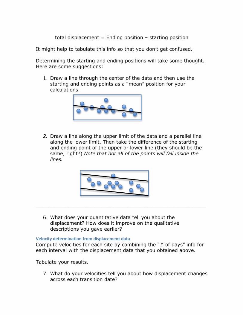
total displacement = Ending position – starting position

It might help to tabulate this info so that you don’t get confused. Determining the starting and ending positions will take some thought. Here are some suggestions:

1. Draw a line through the center of the data and then use the starting and ending points as a “mean” position for your calculations.

2. Draw a line along the upper limit of the data and a parallel line

along the lower limit. Then take the difference of the starting and ending point of the upper or lower line (they should be the same, right?) Note that not all of the points will fall inside the lines.

________________________________________________________

6. What does your quantitative data tell you about the displacement? How does it improve on the qualitative descriptions you gave earlier?

VelocitydeterminationfromdisplacementdataCompute velocities for each site by combining the “# of days” info for each interval with the displacement data that you obtained above. Tabulate your results.

7. What do your velocities tell you about how displacement changes across each transition date?

8. Does it make sense to compare the amount of displacement for

the different intervals? Or is it better to compare velocities? Why or why not? Give specific examples to illustrate your answer.

GraphDisplacementVectors We will make the following graphs:

1. Graph of displacement vectors; one site; all intervals 2. Graph of displacement vectors; all sites; one common interval 3. Graph of velocity vectors; one site; all intervals

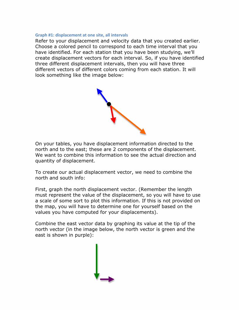
Graph#1:displacementatonesite,allintervalsRefer to your displacement and velocity data that you created earlier. Choose a colored pencil to correspond to each time interval that you have identified. For each station that you have been studying, we’ll create displacement vectors for each interval. So, if you have identified three different displacement intervals, then you will have three different vectors of different colors coming from each station. It will look something like the image below: On your tables, you have displacement information directed to the north and to the east; these are 2 components of the displacement. We want to combine this information to see the actual direction and quantity of displacement. To create our actual displacement vector, we need to combine the north and south info: First, graph the north displacement vector. (Remember the length must represent the value of the displacement, so you will have to use a scale of some sort to plot this information. If this is not provided on the map, you will have to determine one for yourself based on the values you have computed for your displacements). Combine the east vector data by graphing its value at the tip of the north vector (in the image below, the north vector is green and the east is shown in purple):

The final displacement vector (shown in black below) will connect the beginning of the north vector with the tip of the east vector: Now repeat this for your observations. But when you are plotting your north and east vectors, use a plain #2 pencil; use colored pencils for the final displacement vector and erase the north and east vectors when you are done (these will just make your map too complicated).

9. For each time interval that you have studied, use your protractor to determine the direction of motion and measure the vector length to determine the amount. Summarize your results on a table like the one that follows below:

10. Summarize the results in your table with a brief narrative

description of how the site moved over the different time intervals

Graph2:displacementatallsites,onetimeinterval Choose a time interval that all of the sites have in common. Graph the displacement vectors for each site during this interval following the guidelines described above. Complete a table like that you did above so that you can compare all of the results easily.

11. Summarize how these different sites moved relative to one another with a brief narrative description.

Graph3:velocityatonesite,alltimeintervals Return to a single site (can be the one you worked on first. Now graph the velocity vectors for this site over the different time intervals you identified. Again, complete a table like that above so that you can easily compare the different velocities.

12. Summarize the results in your table with a brief narrative description of how the site velocity changed over the different time intervals

Summaryquestionstoponder

13. Which do you like better? The vector graph or the time series? Which makes more sense to you and why? (there is no right answer here; just opinions)

14. Looking at the vertical data for all of the sites, what does it tell you the sites did during the past year? Why would this data be more difficult to work with than the horizontal components of north and east?

15. Can you imagine how these data might change in the days

leading up to or following an eruption? Do you think that this sort of data would be useful in evaluating eruption threat?

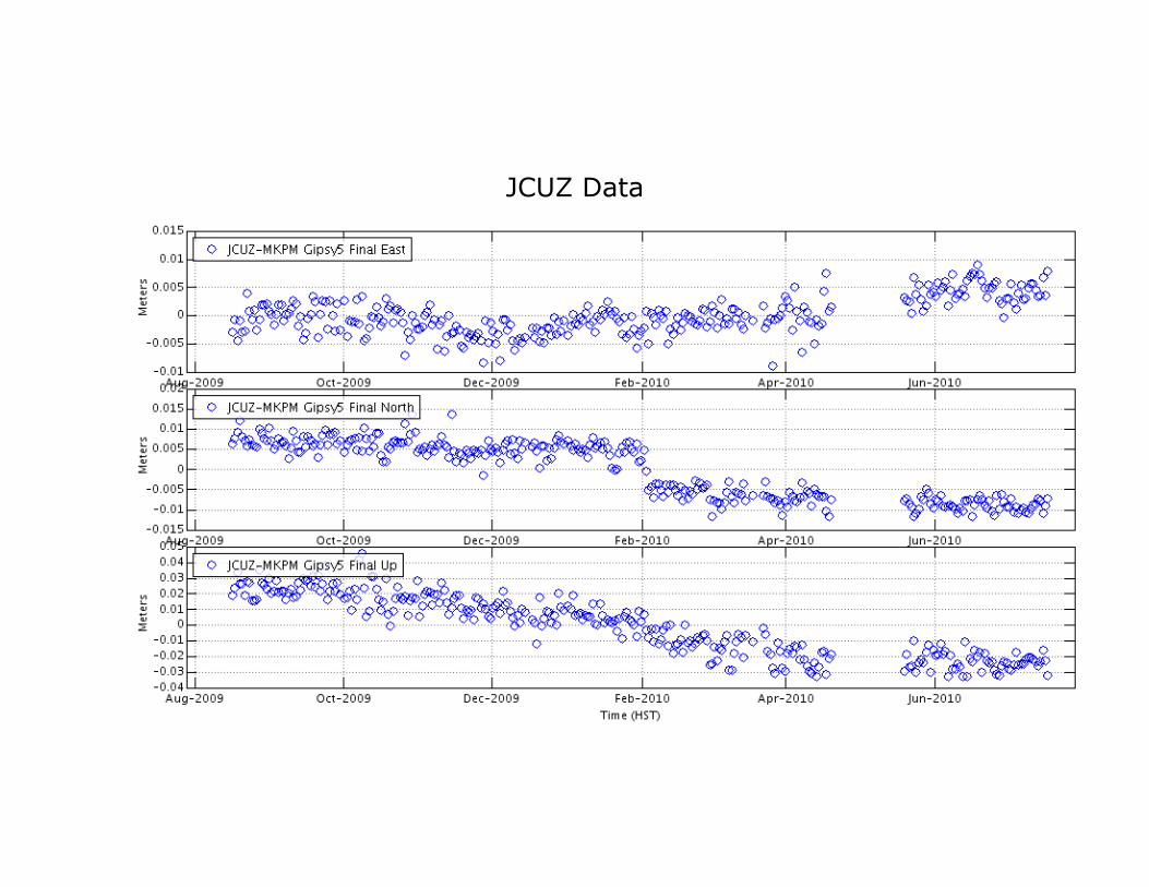
JCUZ Data

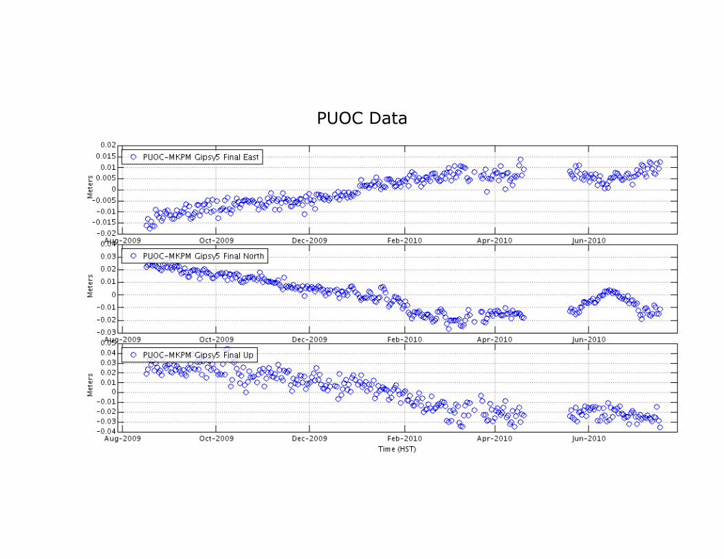
PUOC Data

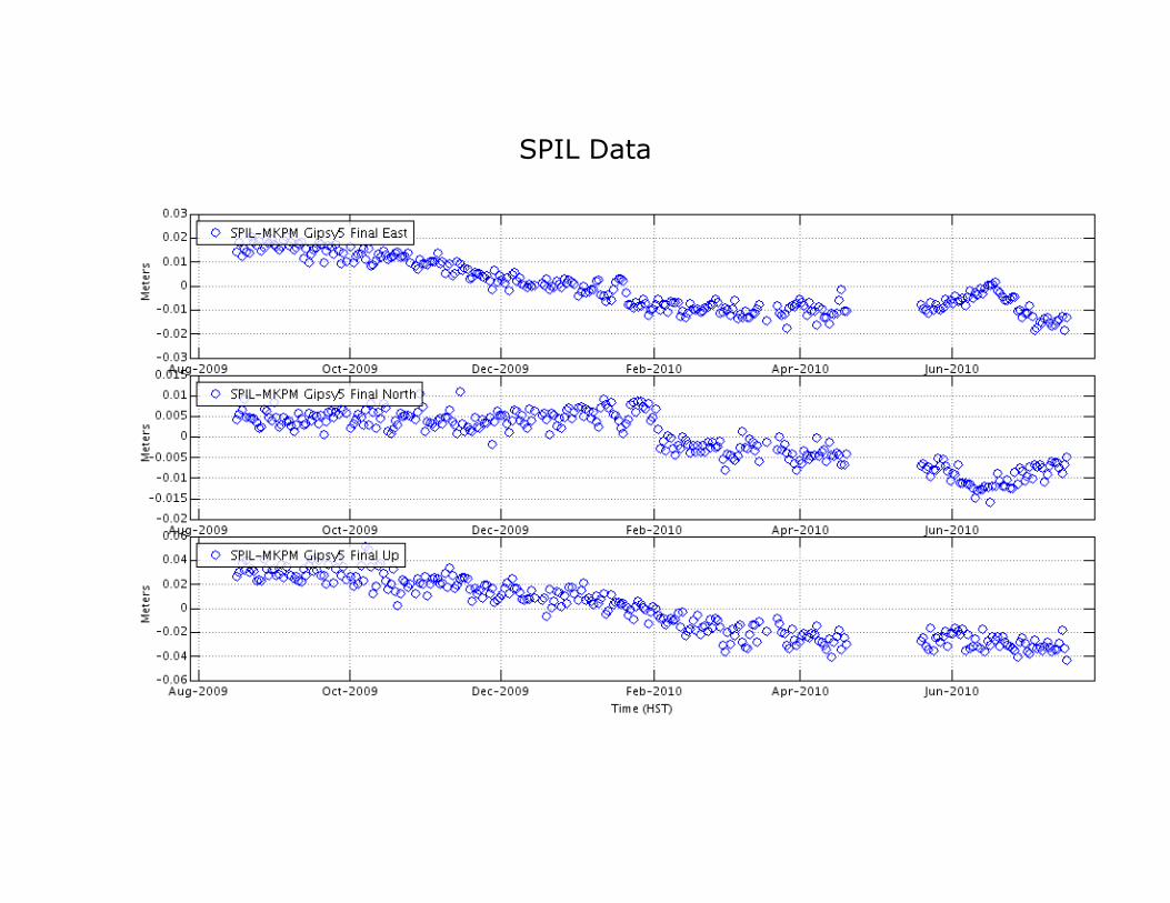
SPIL Data

North