Embed Size (px)
Citation preview
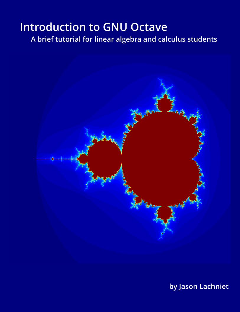
Introduction to GNU OctaveA brief tutorial for linear algebra and calculus students
by Jason Lachniet

Introduction to GNU Octave
A brief tutorial for linear algebra and calculus students
Jason LachnietWytheville Community College
First Edition

iv
v
© 2017 by Jason LachnietISBN 978-1-365-98319-1
This work is licensed under a Creative Commons Attribution-ShareAlike 4.0 International Li-cense. To view a copy of this license, visit http://creativecommons.org/licenses/by-sa/4.0/ or send a letter to Creative Commons, PO Box 1866, Mountain View, CA 94042, USA.
Corrected 1st Ed. (May 12, 2018)

vi
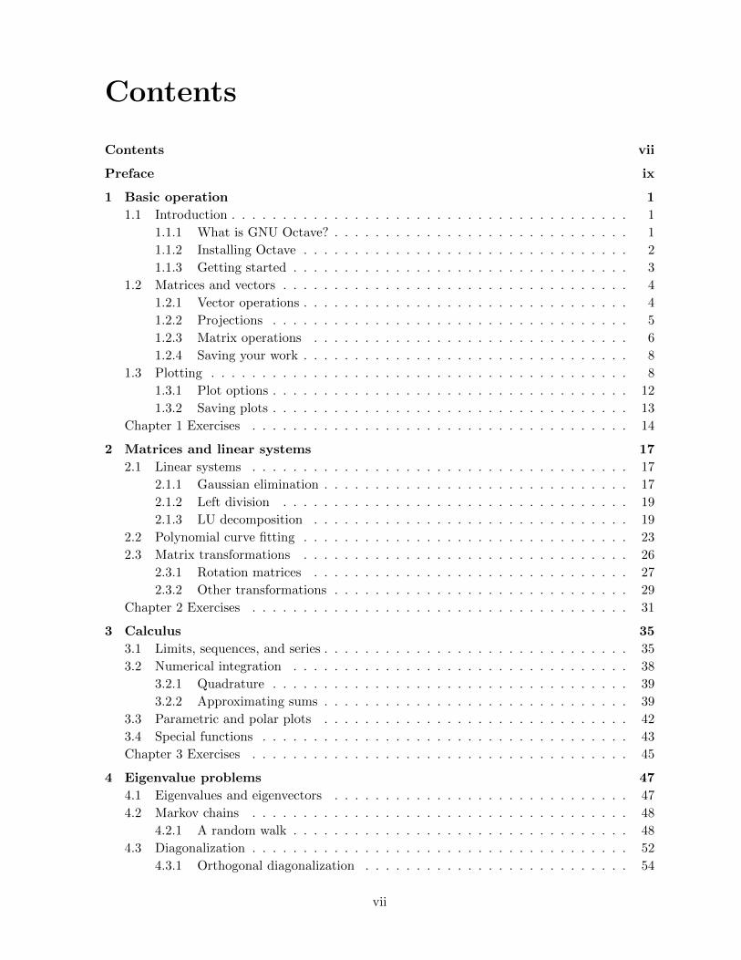
Contents
Contents vii
Preface ix
1 Basic operation 1
1.1 Introduction . . . . . . . . . . . . . . . . . . . . . . . . . . . . . . . . . . . . . . . 1
1.1.1 What is GNU Octave? . . . . . . . . . . . . . . . . . . . . . . . . . . . . . 1
1.1.2 Installing Octave . . . . . . . . . . . . . . . . . . . . . . . . . . . . . . . . 2
1.1.3 Getting started . . . . . . . . . . . . . . . . . . . . . . . . . . . . . . . . . 3
1.2 Matrices and vectors . . . . . . . . . . . . . . . . . . . . . . . . . . . . . . . . . . 4
1.2.1 Vector operations . . . . . . . . . . . . . . . . . . . . . . . . . . . . . . . . 4
1.2.2 Projections . . . . . . . . . . . . . . . . . . . . . . . . . . . . . . . . . . . 5
1.2.3 Matrix operations . . . . . . . . . . . . . . . . . . . . . . . . . . . . . . . 6
1.2.4 Saving your work . . . . . . . . . . . . . . . . . . . . . . . . . . . . . . . . 8
1.3 Plotting . . . . . . . . . . . . . . . . . . . . . . . . . . . . . . . . . . . . . . . . . 8
1.3.1 Plot options . . . . . . . . . . . . . . . . . . . . . . . . . . . . . . . . . . . 12
1.3.2 Saving plots . . . . . . . . . . . . . . . . . . . . . . . . . . . . . . . . . . . 13
Chapter 1 Exercises . . . . . . . . . . . . . . . . . . . . . . . . . . . . . . . . . . . . . 14
2 Matrices and linear systems 17
2.1 Linear systems . . . . . . . . . . . . . . . . . . . . . . . . . . . . . . . . . . . . . 17
2.1.1 Gaussian elimination . . . . . . . . . . . . . . . . . . . . . . . . . . . . . . 17
2.1.2 Left division . . . . . . . . . . . . . . . . . . . . . . . . . . . . . . . . . . 19
2.1.3 LU decomposition . . . . . . . . . . . . . . . . . . . . . . . . . . . . . . . 19
2.2 Polynomial curve fitting . . . . . . . . . . . . . . . . . . . . . . . . . . . . . . . . 23
2.3 Matrix transformations . . . . . . . . . . . . . . . . . . . . . . . . . . . . . . . . 26
2.3.1 Rotation matrices . . . . . . . . . . . . . . . . . . . . . . . . . . . . . . . 27
2.3.2 Other transformations . . . . . . . . . . . . . . . . . . . . . . . . . . . . . 29
Chapter 2 Exercises . . . . . . . . . . . . . . . . . . . . . . . . . . . . . . . . . . . . . 31
3 Calculus 35
3.1 Limits, sequences, and series . . . . . . . . . . . . . . . . . . . . . . . . . . . . . . 35
3.2 Numerical integration . . . . . . . . . . . . . . . . . . . . . . . . . . . . . . . . . 38
3.2.1 Quadrature . . . . . . . . . . . . . . . . . . . . . . . . . . . . . . . . . . . 39
3.2.2 Approximating sums . . . . . . . . . . . . . . . . . . . . . . . . . . . . . . 39
3.3 Parametric and polar plots . . . . . . . . . . . . . . . . . . . . . . . . . . . . . . 42
3.4 Special functions . . . . . . . . . . . . . . . . . . . . . . . . . . . . . . . . . . . . 43
Chapter 3 Exercises . . . . . . . . . . . . . . . . . . . . . . . . . . . . . . . . . . . . . 45
4 Eigenvalue problems 47
4.1 Eigenvalues and eigenvectors . . . . . . . . . . . . . . . . . . . . . . . . . . . . . 47
4.2 Markov chains . . . . . . . . . . . . . . . . . . . . . . . . . . . . . . . . . . . . . 48
4.2.1 A random walk . . . . . . . . . . . . . . . . . . . . . . . . . . . . . . . . . 48
4.3 Diagonalization . . . . . . . . . . . . . . . . . . . . . . . . . . . . . . . . . . . . . 52
4.3.1 Orthogonal diagonalization . . . . . . . . . . . . . . . . . . . . . . . . . . 54
vii
viii CONTENTS
4.4 Singular value decomposition . . . . . . . . . . . . . . . . . . . . . . . . . . . . . 56
4.4.1 Least squares . . . . . . . . . . . . . . . . . . . . . . . . . . . . . . . . . . 59
4.4.2 Image compression . . . . . . . . . . . . . . . . . . . . . . . . . . . . . . . 62
4.5 Gram-Schmidt and the QR algorithm . . . . . . . . . . . . . . . . . . . . . . . . 63
4.5.1 The Gram-Schmidt process . . . . . . . . . . . . . . . . . . . . . . . . . . 63
4.5.2 QR decomposition . . . . . . . . . . . . . . . . . . . . . . . . . . . . . . . 65
4.5.3 The QR algorithm . . . . . . . . . . . . . . . . . . . . . . . . . . . . . . . 67
Chapter 4 Exercises . . . . . . . . . . . . . . . . . . . . . . . . . . . . . . . . . . . . . 69
5 Additional topics 73
5.1 Three dimensional graphs . . . . . . . . . . . . . . . . . . . . . . . . . . . . . . . 73
5.1.1 Space curves . . . . . . . . . . . . . . . . . . . . . . . . . . . . . . . . . . 73
5.1.2 Surfaces . . . . . . . . . . . . . . . . . . . . . . . . . . . . . . . . . . . . . 75
5.1.3 Solids of revolution . . . . . . . . . . . . . . . . . . . . . . . . . . . . . . . 76
5.2 Multiple integrals . . . . . . . . . . . . . . . . . . . . . . . . . . . . . . . . . . . . 77
5.2.1 Double Riemann sums . . . . . . . . . . . . . . . . . . . . . . . . . . . . . 82
5.3 Vector fields . . . . . . . . . . . . . . . . . . . . . . . . . . . . . . . . . . . . . . . 84
5.4 Statistics . . . . . . . . . . . . . . . . . . . . . . . . . . . . . . . . . . . . . . . . 86
5.5 Differential equations . . . . . . . . . . . . . . . . . . . . . . . . . . . . . . . . . . 90
5.5.1 Slope fields . . . . . . . . . . . . . . . . . . . . . . . . . . . . . . . . . . . 90
5.5.2 Euler’s method . . . . . . . . . . . . . . . . . . . . . . . . . . . . . . . . . 91
5.5.3 The Livermore solver . . . . . . . . . . . . . . . . . . . . . . . . . . . . . . 93
Chapter 5 Exercises . . . . . . . . . . . . . . . . . . . . . . . . . . . . . . . . . . . . . 95
A MATLAB compatibility 97
B List of Octave commands 99
References 103
Index 105
Preface
These notes are not intended as a comprehensive manual. Instead, what follows is a tutorialthat puts Octave to work solving a selection of applied problems in linear algebra and calculus.The goal is to learn enough of the basics to begin solving problems with minimum frustration.Note that minimum frustration does not mean no frustration. Be patient!
Features of the text
To get the most out of this book, you should read it alongside an open Octave window whereyou can follow along with the computations (you will want paper and pencil, too, as well as yourmath books). Blocks of Octave commands are indented and printed with special formatting asfollows.
>> % example Octave commands :>>>> x = [−3 : 0 . 1 : 3 ] ;>> p lo t (x , x . ˆ 2 ) ;>> t i t l e ( 'Example p l o t ' )
Comments used to explain the code are preceded by a “%” sign and shown in green. Keywords are highlighted in magenta. Strings (text variables) are highlighted in purple. The sameformatting is used for commands that appear inline in the text. The Octave prompt is shownas “>>”.
Octave scripts (.m-files) are shown between horizontal rules and are labeled with a title, as inthe following example. These are short programs in the Octave language.
Octave Script 1: Example
1 % This i s an example Octave s c r i p t ( .m− f i l e )2 t = l i n s p a c e (0 , 2*pi , 50) ;3 x = cos ( t ) ;4 y = s i n ( t ) ;5
6 % plo t the graph o f a un i t c i r c l e7 p lo t (x , y ) ;8 g r id on ;
The line numbers are for reference purposes and are not part of the code.
ix
x PREFACE
The color coding is not essential to understand the text. Thus the text can be printed in blackand white to save on printing costs.
If you are reading the electronic PDF version, there are numerous hyperlinks throughout thetext that link back to other parts of the text, or to external urls. There is a set of bookmarks toeach chapter and section that can be used to easily navigate from section to section. Open thebookmark link at the left side of the screen in your PDF viewer to use this feature (not visiblein a web browser view; use a full PDF reader, like https://get.adobe.com/reader/).
Solutions to the many example problems are offset with a bar along the left side of the page,as shown here. A box signifies the end of the example.
MATLAB
The majority of the code shown in this book will work in MATLAB. This guide can thereforealso be used an introduction to that software package. Refer to Appendix A for some notes onMATLAB compatibility.
Scope and purpose
This guide is heavy on linear algebra and makes a good supplement to a linear algebra textbook.But, it is assumed that any college student studying linear algebra will also be studying calculusand differential equations, maybe statistics. Therefore it makes sense to apply the Octave skillslearned for linear algebra to these subjects as well. Chapters 3 and 5 have several applicationsto calculus, differential equations, and statistics. The overarching objective is to enhance ourunderstanding of calculus and linear algebra using Octave as a tool for computations. For themost part, we will not address issues of accuracy and round-off error in machine arithmetic.For more details about numerical issues, refer to [1], which also contains many useful Octaveexamples.
To get started, read Chapter 1, without worrying too much about any of the mathematics youdon’t yet understand. After grasping the basics, you should be able to move into any of thechapters or sections that interest you.
Every chapter concludes with a set of problems, some of which are routine practice, and someof which are more extended applied projects.
Most examples assume the reader is familiar with the mathematics involved. In a few cases,more detailed explanation of relevant theorems is given by way of motivation, but there are noproofs. Refer to the linear algebra and calculus books listed in the references for background onthe underlying mathematics. In the spirit of openness, all references listed are available for freeunder GNU or Creative Commons licenses and can be accessed using the links provided.
Chapter 1
Basic operation
1.1 Introduction
1.1.1 What is GNU Octave?
GNU Octave is free software designed for scientific computing. It is intended primarily forsolving numerical problems. In linear algebra, we will use Octave’s capabilities to solve systemsof linear equations and to work with matrices and vectors. Octave can also generate sophisticatedplots. For example, we will use it in vector calculus to plot vector fields, space curves, andthree dimensional surfaces. Octave is mostly compatible with the popular “industry standard”commercial software package MATLAB, so the skills you learn here can be applied to MATLABprogramming as well. In fact, while this guide is written and intended as an introduction toOctave, it can serve equally well as a basic introduction to MATLAB.
What is GNU? A gnu is a type of antelope, but GNU is a free, UNIX-like computer operatingsystem. GNU is a recursive acronym that stands for “GNU’s not Unix.” GNU Octave (andmany other free programs) are licensed under the GNU General Public License: http://www.
gnu.org/licenses/gpl.html.
From www.gnu.org/software/octave:
GNU Octave is a high-level interpreted language, primarily intended for numericalcomputations. It provides capabilities for the numerical solution of linear and non-linear problems, and for performing other numerical experiments. It also providesextensive graphics capabilities for data visualization and manipulation. Octave isnormally used through its interactive command line interface, but it can also beused to write non-interactive programs. The Octave language is quite similar toMATLAB so that most programs are easily portable.
Octave is a fully functioning programming language, but it is not a general purpose programminglanguage (like C or Java). Octave is numerical, not symbolic; it is not a computer algebra system
1
2 CHAPTER 1. BASIC OPERATION
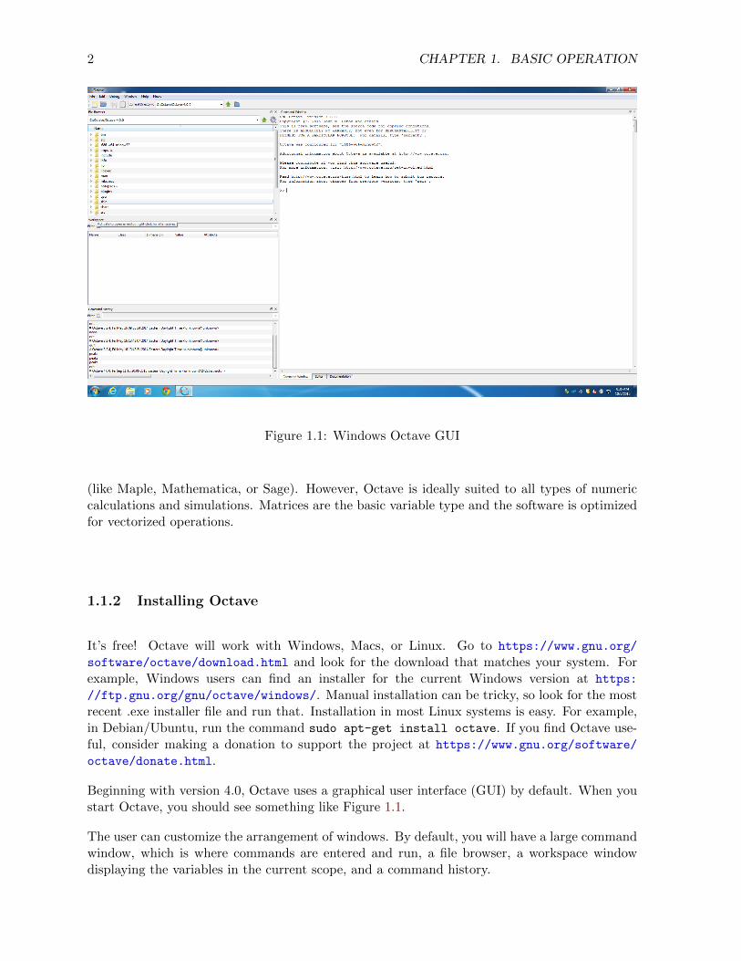
Figure 1.1: Windows Octave GUI
(like Maple, Mathematica, or Sage). However, Octave is ideally suited to all types of numericcalculations and simulations. Matrices are the basic variable type and the software is optimizedfor vectorized operations.
1.1.2 Installing Octave
It’s free! Octave will work with Windows, Macs, or Linux. Go to https://www.gnu.org/
software/octave/download.html and look for the download that matches your system. Forexample, Windows users can find an installer for the current Windows version at https:
//ftp.gnu.org/gnu/octave/windows/. Manual installation can be tricky, so look for the mostrecent .exe installer file and run that. Installation in most Linux systems is easy. For example,in Debian/Ubuntu, run the command sudo apt-get install octave. If you find Octave use-ful, consider making a donation to support the project at https://www.gnu.org/software/
octave/donate.html.
Beginning with version 4.0, Octave uses a graphical user interface (GUI) by default. When youstart Octave, you should see something like Figure 1.1.
The user can customize the arrangement of windows. By default, you will have a large commandwindow, which is where commands are entered and run, a file browser, a workspace windowdisplaying the variables in the current scope, and a command history.
1.1. INTRODUCTION 3
1.1.3 Getting started
There are several good help resources on the web, and built-in help functions within Octave.The shell command help can be used at the Octave prompt. In particular, if you know the nameof the command you want to use, help NAME will give the correct syntax.
Here are two good free, online resources:
� The Octave Manual [3]:http://www.gnu.org/software/octave/octave.pdf
� Wikibooks Tutorial:https://en.wikibooks.org/wiki/Octave_Programming_Tutorial
Additional help can be found with internet searches. Depending on what you are looking for,searches for Octave commands and searches for MATLAB commands can both be useful. Nu-merous commercial user’s guides and textbooks for Octave and/or MATLAB are available.Linear algebra textbooks sometimes contain MATLAB code examples and these generally workin Octave as well.
The best way to get started is to try some simple problems. Use the following examples asa tutorial to learn your way around the program. Octave knows about basic arithmetic. Trysomething simple like:
>> 2*6 + (7 − 4) ˆ2ans = 21
Octave ignores white space, so 2*6 and 2 * 6 are interpreted the same way. You can’t takeshortcuts and leave out implied operations, though. For example, 2(5 − 1) will give an error.Use 2*(5 − 1).
Vectors and matrices are basic variable types, so it is easier to learn Octave syntax if you alreadyknow a little linear algebra. Try this example to enter a row vector and name it u. You do notneed to enter the comments (indicated by the % sign).
>> u = [ 1 −4 6 ] % row vecto ru = % v a r i a b l e name
1 −4 6 % output
The code u = . . . assigns the result of the operation that follows to the variable u, which canthen be recalled and used in further calculations.
To create a column vector instead, use semicolons:
>> u = [ 1 ; −4; 6 ] % column vecto ru = % v a r i a b l e name
1 % output−4
6
4 CHAPTER 1. BASIC OPERATION
Notice that the function of the semicolon is to begin a new row. The same basic syntax is usedto enter matrices. For example, let’s see how to enter a matrix:
>> A = [ 1 2 −3; 2 4 0 ; 1 1 1 ] % matrixA = % v a r i a b l e name
1 2 −3 % output2 4 01 1 1
1.2 Matrices and vectors
Matrices are the basic variable type in Octave. In fact, a scalar is treated as a 1 × 1 matrix.Similarly, a row vector is a 1× n matrix and a column vector is an m× 1 matrix.
1.2.1 Vector operations
We’ll start with some simple examples. First, enter the column vector u from above, if it is notalready in memory.
>> u = [ 1 ; −4; 6 ]u =
1−4
6
Now enter another column vector v and try the following vector operations which illustratelinear combinations, dot product, cross product, and norm.
>> v = [ 2 ; 1 ; −1]v =
21−1
>> 2*v + 3*uans =
7−10
16
>> dot (u , v ) % dot productans = −8
>> c r o s s (u , v ) % c r o s s product
1.2. MATRICES AND VECTORS 5
ans =
−213
9
>> norm(u) % length o f vec to r uans = 7.2801
Try a few more operations:
� Find cross(v, u). How does that compare to u× v?
� Calculate the length of v, ||v||, using norm(v).
� Create a unit vector v1 that points in the direction of v.
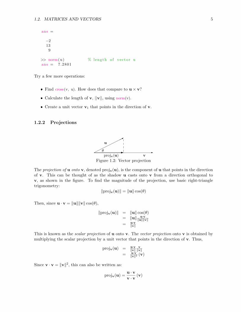
1.2.2 Projections
-�����
���*
-θ
u
projv(u) v
Figure 1.2: Vector projection
The projection of u onto v, denoted projv(u), is the component of u that points in the directionof v. This can be thought of as the shadow u casts onto v from a direction orthogonal tov, as shown in the figure. To find the magnitude of the projection, use basic right-triangletrigonometry:
‖projv(u)‖ = ‖u‖ cos(θ)
Then, since u · v = ‖u‖‖v‖ cos(θ),
‖projv(u)‖ = ‖u‖ cos(θ)= ‖u‖ u·v
‖u‖‖v‖= u·v
‖v‖
This is known as the scalar projection of u onto v. The vector projection onto v is obtained bymultiplying the scalar projection by a unit vector that points in the direction of v. Thus,
projv(u) = u·v‖v‖
v‖v‖
= u·v‖v‖2 (v)
Since v · v = ‖v‖2, this can also be written as:
projv(u) =u · vv · v
(v)
6 CHAPTER 1. BASIC OPERATION
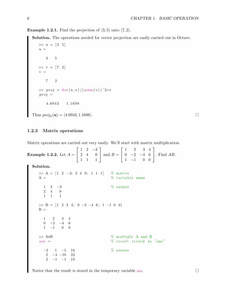
Example 1.2.1. Find the projection of 〈3, 5〉 onto 〈7, 2〉.
Solution. The operations needed for vector projection are easily carried out in Octave.
>> u = [ 3 5 ]u =
3 5
>> v = [ 7 2 ]v =
7 2
>> pro j = dot (u , v ) /(norm( v ) ) ˆ2*vpro j =
4.0943 1 .1698
Thus projv(u) = 〈4.0943, 1.1698〉.
1.2.3 Matrix operations
Matrix operations are carried out very easily. We’ll start with matrix multiplication.
Example 1.2.2. Let A =
1 2 −32 4 01 1 1
and B =
1 2 3 40 −2 −4 61 −1 0 0
. Find AB.
Solution.
>> A = [ 1 2 −3; 2 4 0 ; 1 1 1 ] % matrixA = % v a r i a b l e name
1 2 −3 % output2 4 01 1 1
>> B = [ 1 2 3 4 ; 0 −2 −4 6 ; 1 −1 0 0 ]B =
1 2 3 40 −2 −4 61 −1 0 0
>> A*B % mult ip ly A and Bans = % r e s u l t s to r ed as ' ans '
−2 1 −5 16 % answer2 −4 −10 322 −1 −1 10
Notice that the result is stored in the temporary variable ans.
1.2. MATRICES AND VECTORS 7
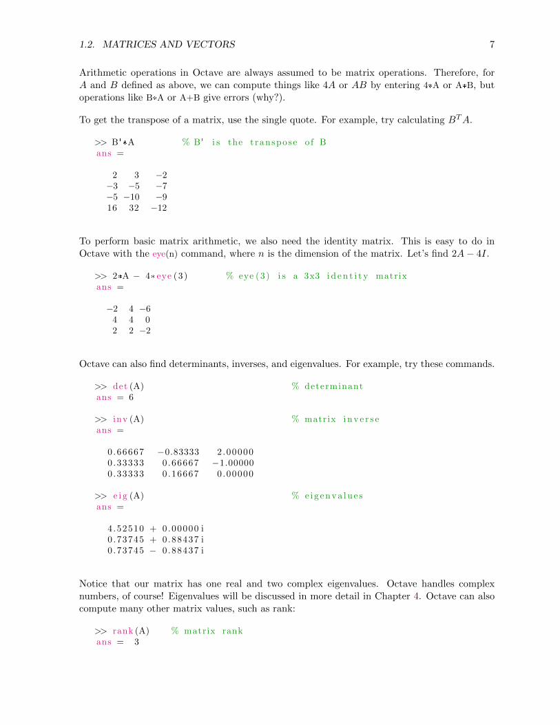
Arithmetic operations in Octave are always assumed to be matrix operations. Therefore, forA and B defined as above, we can compute things like 4A or AB by entering 4*A or A*B, butoperations like B*A or A+B give errors (why?).
To get the transpose of a matrix, use the single quote. For example, try calculating BTA.
>> B' *A % B ' i s the t ranspose o f Bans =
2 3 −2−3 −5 −7−5 −10 −916 32 −12
To perform basic matrix arithmetic, we also need the identity matrix. This is easy to do inOctave with the eye(n) command, where n is the dimension of the matrix. Let’s find 2A− 4I.
>> 2*A − 4* eye (3 ) % eye (3 ) i s a 3x3 i d e n t i t y matrixans =
−2 4 −64 4 02 2 −2
Octave can also find determinants, inverses, and eigenvalues. For example, try these commands.
>> det (A) % determinantans = 6
>> inv (A) % matrix i n v e r s eans =
0.66667 −0.83333 2.000000.33333 0.66667 −1.000000.33333 0.16667 0.00000
>> e i g (A) % e i g e n v a l u e sans =
4.52510 + 0.00000 i0 .73745 + 0.88437 i0 .73745 − 0.88437 i
Notice that our matrix has one real and two complex eigenvalues. Octave handles complexnumbers, of course! Eigenvalues will be discussed in more detail in Chapter 4. Octave can alsocompute many other matrix values, such as rank:
>> rank (A) % matrix rankans = 3
8 CHAPTER 1. BASIC OPERATION
1.2.4 Saving your work
If we have solved some problems, we are going to want some way to save our work and maybereload it later. In Octave, you can save variables that you defined in your session, but you cannotsave the commands you used or a whole worksheet. Octave does have a command history thatpersists between sessions, so past commands can be brought up using the up arrow key, or usingthe command history list in the GUI. If you want to document how you did something, use copyand paste to copy your commands into a Word document or text file.
Within the Octave graphical user interface, you should see your current directory listed nearthe top left. You can click the folder button to navigate to a different directory, such as thedesktop or your personal flash drive. Under the file menu, the option “save workspace as” willsave all of your current variables in a file of your choosing. You can see a list of the variablescurrently defined listed under “workspace” on the left side of the screen. You can use the “loadworkspace” option under the file menu to load previously saved variables.
Another approach is to use the manual save and load commands at the command line. If youtype save FILENAME var1 var2 ..., Octave will save the specified variables in the file FILENAME.If you do not supply a list of variables, then all variables in the current scope will be saved. Youcan then reload the saved variable(s) at another time by navigating to the appropriate directoryand using load FILENAME. You can also load a variable or workspace by double-clicking on itsname in the file browser.
If you want to save a series of commands that can be reopened and run again, you can createan Octave script, also known as an .m-file. This will be described in more detail in Chapter 3.
1.3 Plotting
Basic two-dimensional plotting of functions in Octave is accomplished by creating a vector forthe independent variable and a second vector for the range of the function. There are severalforms for the syntax and we will attempt to outline the simplest methods here. See also:
� http://www.gnu.org/software/octave/doc/interpreter/Plotting.html
� http://en.wikibooks.org/wiki/Octave_Programming_Tutorial/Plotting
Let’s start by plotting the graph of the function sin(x) on the interval [0, 2π]. Like a typicalgraphing calculator, Octave will simply plot a series of points and connect the dots to representthe curve. The process is less automated in Octave (but in the end, much more powerful). Webegin by creating a vector of x-values.
>> x = l i n s p a c e (0 , 2*pi , 50) ;
Notice the format linspace( start val , end val, n). This creates a row vector of 50 evenly spacedvalues beginning at 0 and going up to 2π. The smaller the increment, the smoother the curvewill look. In this case, 50 points should be suitable. The semicolon at the end of the line is to
1.3. PLOTTING 9
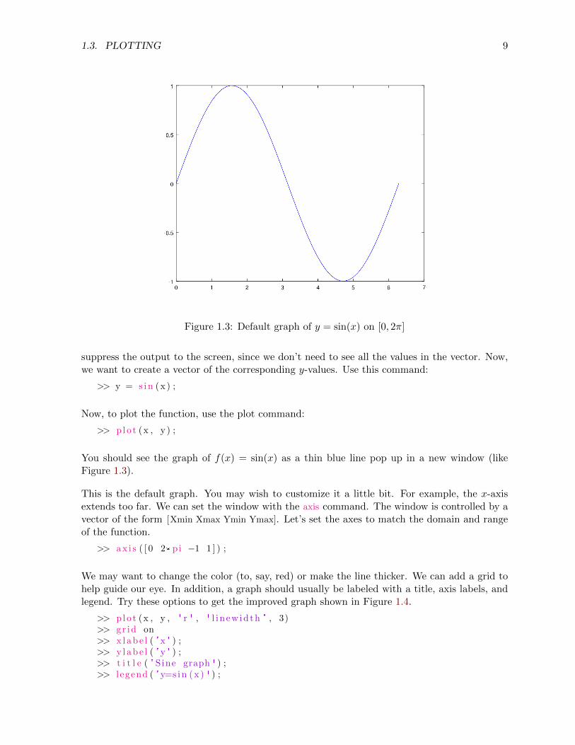
Figure 1.3: Default graph of y = sin(x) on [0, 2π]
suppress the output to the screen, since we don’t need to see all the values in the vector. Now,we want to create a vector of the corresponding y-values. Use this command:
>> y = s i n ( x ) ;
Now, to plot the function, use the plot command:
>> p lo t (x , y ) ;
You should see the graph of f(x) = sin(x) as a thin blue line pop up in a new window (likeFigure 1.3).
This is the default graph. You may wish to customize it a little bit. For example, the x-axisextends too far. We can set the window with the axis command. The window is controlled by avector of the form [Xmin Xmax Ymin Ymax]. Let’s set the axes to match the domain and rangeof the function.
>> a x i s ( [ 0 2* pi −1 1 ] ) ;
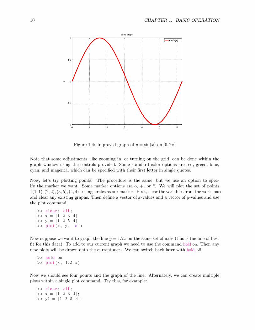
We may want to change the color (to, say, red) or make the line thicker. We can add a grid tohelp guide our eye. In addition, a graph should usually be labeled with a title, axis labels, andlegend. Try these options to get the improved graph shown in Figure 1.4.
>> p lo t (x , y , ' r ' , ' l i n ew id th ' , 3)>> g r id on>> x l a b e l ( 'x ' ) ;>> y l a b e l ( 'y ' ) ;>> t i t l e ( ' Sine graph ' ) ;>> l egend ( 'y=s i n ( x ) ' ) ;
10 CHAPTER 1. BASIC OPERATION
Figure 1.4: Improved graph of y = sin(x) on [0, 2π]
Note that some adjustments, like zooming in, or turning on the grid, can be done within thegraph window using the controls provided. Some standard color options are red, green, blue,cyan, and magenta, which can be specified with their first letter in single quotes.
Now, let’s try plotting points. The procedure is the same, but we use an option to spec-ify the marker we want. Some marker options are o, +, or *. We will plot the set of points{(1, 1), (2, 2), (3, 5), (4, 4)} using circles as our marker. First, clear the variables from the workspaceand clear any existing graphs. Then define a vector of x-values and a vector of y-values and usethe plot command.
>> c l e a r ; c l f ;>> x = [ 1 2 3 4 ]>> y = [ 1 2 5 4 ]>> p lo t (x , y , ' o ' )
Now suppose we want to graph the line y = 1.2x on the same set of axes (this is the line of bestfit for this data). To add to our current graph we need to use the command hold on. Then anynew plots will be drawn onto the current axes. We can switch back later with hold off .
>> hold on>> p lo t (x , 1 .2* x )
Now we should see four points and the graph of the line. Alternately, we can create multipleplots within a single plot command. Try this, for example:
>> c l e a r ; c l f ;>> x = [ 1 2 3 4 ] ;>> y1 = [ 1 2 5 4 ] ;
1.3. PLOTTING 11
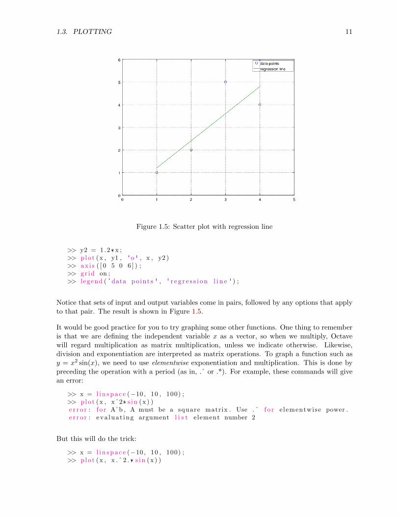
Figure 1.5: Scatter plot with regression line
>> y2 = 1.2* x ;>> p lo t (x , y1 , ' o ' , x , y2 )>> a x i s ( [ 0 5 0 6 ] ) ;>> g r id on ;>> l egend ( ' data po in t s ' , ' r e g r e s s i o n l i n e ' ) ;
Notice that sets of input and output variables come in pairs, followed by any options that applyto that pair. The result is shown in Figure 1.5.
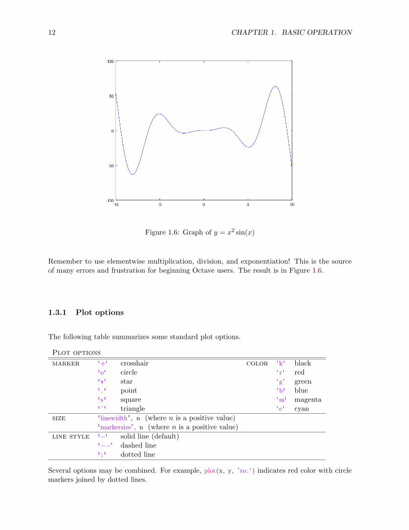
It would be good practice for you to try graphing some other functions. One thing to rememberis that we are defining the independent variable x as a vector, so when we multiply, Octavewill regard multiplication as matrix multiplication, unless we indicate otherwise. Likewise,division and exponentiation are interpreted as matrix operations. To graph a function such asy = x2 sin(x), we need to use elementwise exponentiation and multiplication. This is done bypreceding the operation with a period (as in, .ˆ or .*). For example, these commands will givean error:
>> x = l i n s p a c e (−10 , 10 , 100) ;>> p lo t (x , xˆ2* s i n ( x ) )e r r o r : f o r Aˆb , A must be a square matrix . Use . ˆ f o r e lementwise power .e r r o r : eva lua t ing argument l i s t element number 2
But this will do the trick:
>> x = l i n s p a c e (−10 , 10 , 100) ;>> p lo t (x , x . ˆ 2 . * s i n ( x ) )
12 CHAPTER 1. BASIC OPERATION
Figure 1.6: Graph of y = x2 sin(x)
Remember to use elementwise multiplication, division, and exponentiation! This is the sourceof many errors and frustration for beginning Octave users. The result is in Figure 1.6.
1.3.1 Plot options
The following table summarizes some standard plot options.
Plot options
marker '+' crosshair color 'k' black'o' circle 'r ' red'*' star 'g' green' . ' point 'b' blue's ' square 'm' magenta'ˆ' triangle 'c ' cyan
size ' linewidth' , n (where n is a positive value)'markersize' , n (where n is a positive value)
line style '−' solid line (default)'−−' dashed line' : ' dotted line
Several options may be combined. For example, plot(x, y, 'ro: ' ) indicates red color with circlemarkers joined by dotted lines.
1.3. PLOTTING 13
1.3.2 Saving plots
If we have created a good plot, we probably want to save it. The easiest option is to use copyand paste from the plot window. You can also use the “save as” option under the file menu tosave the plot as a PDF.
An alternate method is to save the plot directly by “printing” it to a file. Octave supportsseveral image formats. In the example below, the PNG format is used. To save the currentgraph as a PNG, use this syntax:
>> pr in t f i l ename . png −dpng
Here “filename” is whatever file name you want. You can replace “png” with other imageformats, such as “jpg” or “eps.” Your file will be saved in your current working directory.
14 CHAPTER 1. BASIC OPERATION
Chapter 1 Exercises
Begin each problem with no variables stored. You can clear any previous results with thecommand clear .
1. For practice saving and loading variables, try the following.
(a) Create a new directory called “octave projects”.
(b) Change to the octave projects directory.
(c) Save the example matrices A and B from above in a text file named “matrices.txt”.
(d) Quit Octave.
(e) Restart Octave and reload the saved matrices.
2. Let a = 〈2,−4, 0〉 and b = 〈3, 1.5,−7〉. Find each of the following.
(a) x = 2a + 5b
(b) d = a · b(c) l = ||a||(d) Find a vector n orthogonal to both a and b.
(e) Find projb(a).
Be sure to use the variable names indicated to store your answers. Save your workspaceincluding all of the required variables. What does the dot product reveal about a and b?How did you produce a vector mutually orthogonal to a and b?
3. Begin this problem with no variables stored. Enter the following matrices.
A =
1 −3 52 −4 30 1 −1
, B =
1 −1 0 0−3 0 7 −62 1 −2 −1
, and I3 =
1 0 00 1 00 0 1
.Use Octave to compute each of the following, if possible, or explain why the operation isundefined.
(a) d = det(A)
(b) C = 2A+ 4I
(c) D = A−1
(d) E = B−1
(e) F = BA
(f) G = (AB)T
(g) H = BTAT
Use the variable names indicated to store your answers. Save your workspace includingall of the required variables. Which of the operations were undefined and why? Did younotice anything about (AB)T and BTAT ? If so, explain the relationship between thesequantities.
EXERCISES 15
4. Modify the plot of y = x2 sin(x) given in Figure 1.6 as follows:
(a) Make the graph of y = x2 sin(x) a thick red line.
(b) Graph y = x2 and y = −x2 on the same axes, as thin black dotted lines.
(c) Use a legend to identify each curve.
(d) Add a title.
(e) Add a grid.
(f) Save the plot as a PNG or JPG image file.

16 CHAPTER 1. BASIC OPERATION
Chapter 2
Matrices and linear systems
Octave is a powerful tool for many problems in linear algebra. We have already seen some of thebasics in Section 1.2. In this chapter, we will consider systems of linear equations, polynomialcurve fitting, and rotation matrices.
2.1 Linear systems
2.1.1 Gaussian elimination
Octave has sophisticated algorithms built in for solving systems of linear equations, but it isuseful to start with the more basic process of Gaussian elimination. Using Octave for Gaus-sian elimination lets us practice the procedure, without the inevitable arithmetic errors thatcome when doing elimination by hand. It also teaches useful Octave syntax and methods formanipulating matrices.
Row operations are easy to carry out. But first, we need to see how matrices and vectors areindexed in Octave. Consider the following augmented matrix.
>> B = [ 1 2 3 4 ; 0 −2 −4 6 ; 1 −1 0 0 ]B =
1 2 3 40 −2 −4 61 −1 0 0
If we enter B(2, 3), then the result given is −4. This is the scalar stored in row 2, column 3. Wecan also pull out an entire row vector or column vector using the colon operator. A colon canbe used to specify a limited range, or if no starting or ending value is specified, it gives the fullrange. For example, B(1, :) will give every entry out of the first row.
>> B(1 , : )ans =
17
18 CHAPTER 2. MATRICES AND LINEAR SYSTEMS
1 2 3 4
Now, let’s use this notation to carry out basic row operations on B to reach row-echelon form.
Example 2.1.1. Let
B =
1 2 3 40 −2 −4 61 −1 0 0
Use row operations to put B into row-echelon form, then solve by backward substitution. Com-pare to the row-reduced echelon form computed by Octave.
Solution. The first operation is to replace row 3 with −1 times row 1, added to row 3.
>> B(3 , : ) = (−1)*B(1 , : ) + B(3 , : )ans =
1 2 3 40 −2 −4 60 −3 −3 −4
Next, we will replace row 3 with −1.5 times row 2, added to row 3.
>> B(3 , : ) = −1.5*B(2 , : ) + B(3 , : )ans =
1 2 3 40 −2 −4 60 0 3 −13
The matrix is now in row echelon form. We could continue using row operations to reachrow-reduced echelon form, but it is more efficient to simply write out the correspondinglinear system on paper and solve by backward substitution. Do it! The solution vector is〈173 ,
173 ,−
133 〉. Of course, Octave also has a built-in command to find the row-reduced echelon
form of the matrix directly. Try rref (B) to see the result.
>> r r e f (B)ans =
1.00000 0.00000 0.00000 5.666670.00000 1.00000 0.00000 5.666670.00000 0.00000 1.00000 −4.33333
From here, the solution to the system is evident. Notice that everything is now expressedas floating point numbers (i.e., decimals). Five decimal places are displayed by default. Thevariables are actually stored with higher precision and it is possible to display more decimalplaces, if desired (type format(long)).
2.1. LINEAR SYSTEMS 19
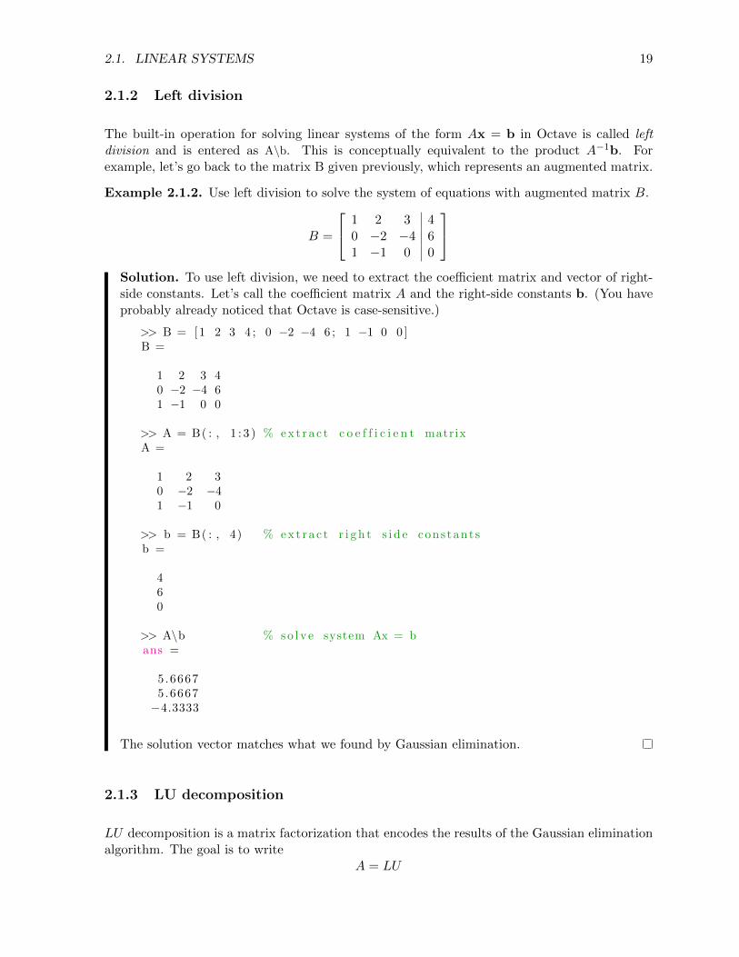
2.1.2 Left division
The built-in operation for solving linear systems of the form Ax = b in Octave is called leftdivision and is entered as A\b. This is conceptually equivalent to the product A−1b. Forexample, let’s go back to the matrix B given previously, which represents an augmented matrix.
Example 2.1.2. Use left division to solve the system of equations with augmented matrix B.
B =
1 2 3 40 −2 −4 61 −1 0 0
Solution. To use left division, we need to extract the coefficient matrix and vector of right-side constants. Let’s call the coefficient matrix A and the right-side constants b. (You haveprobably already noticed that Octave is case-sensitive.)
>> B = [ 1 2 3 4 ; 0 −2 −4 6 ; 1 −1 0 0 ]B =
1 2 3 40 −2 −4 61 −1 0 0
>> A = B( : , 1 : 3 ) % e x t r a c t c o e f f i c i e n t matrixA =
1 2 30 −2 −41 −1 0
>> b = B( : , 4) % e x t r a c t r i g h t s i d e cons tant sb =
460
>> A\b % s o l v e system Ax = bans =
5.66675 .6667−4.3333
The solution vector matches what we found by Gaussian elimination.
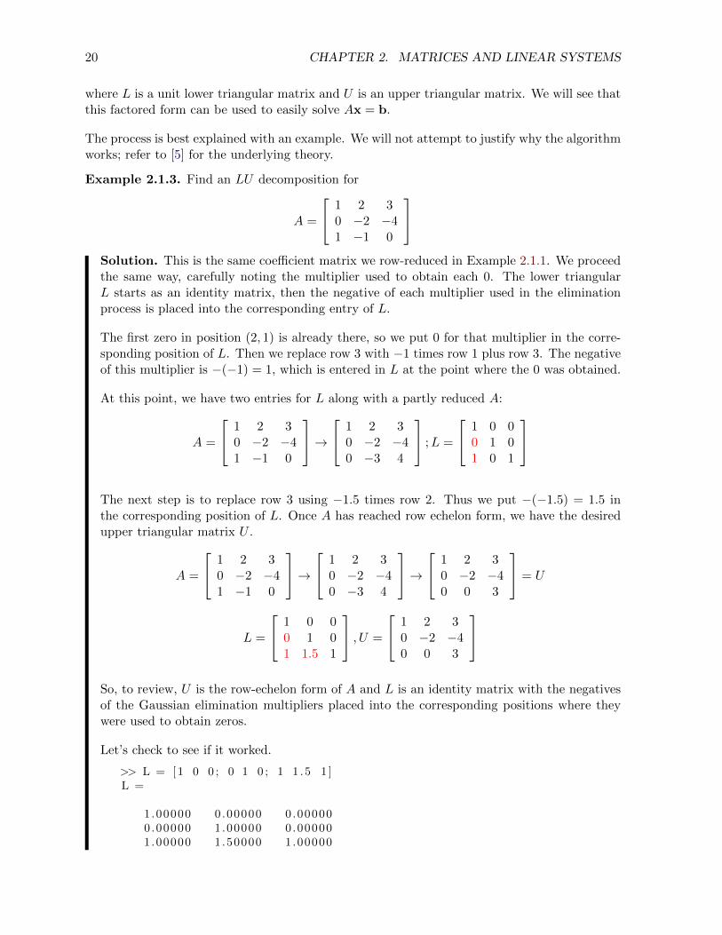
2.1.3 LU decomposition
LU decomposition is a matrix factorization that encodes the results of the Gaussian eliminationalgorithm. The goal is to write
A = LU
20 CHAPTER 2. MATRICES AND LINEAR SYSTEMS
where L is a unit lower triangular matrix and U is an upper triangular matrix. We will see thatthis factored form can be used to easily solve Ax = b.
The process is best explained with an example. We will not attempt to justify why the algorithmworks; refer to [5] for the underlying theory.
Example 2.1.3. Find an LU decomposition for
A =
1 2 30 −2 −41 −1 0
Solution. This is the same coefficient matrix we row-reduced in Example 2.1.1. We proceedthe same way, carefully noting the multiplier used to obtain each 0. The lower triangularL starts as an identity matrix, then the negative of each multiplier used in the eliminationprocess is placed into the corresponding entry of L.
The first zero in position (2, 1) is already there, so we put 0 for that multiplier in the corre-sponding position of L. Then we replace row 3 with −1 times row 1 plus row 3. The negativeof this multiplier is −(−1) = 1, which is entered in L at the point where the 0 was obtained.
At this point, we have two entries for L along with a partly reduced A:
A =
1 2 30 −2 −41 −1 0
→ 1 2 3
0 −2 −40 −3 4
;L =
1 0 00 1 01 0 1
The next step is to replace row 3 using −1.5 times row 2. Thus we put −(−1.5) = 1.5 inthe corresponding position of L. Once A has reached row echelon form, we have the desiredupper triangular matrix U .
A =
1 2 30 −2 −41 −1 0
→ 1 2 3
0 −2 −40 −3 4
→ 1 2 3
0 −2 −40 0 3
= U
L =
1 0 00 1 01 1.5 1
, U =
1 2 30 −2 −40 0 3
So, to review, U is the row-echelon form of A and L is an identity matrix with the negativesof the Gaussian elimination multipliers placed into the corresponding positions where theywere used to obtain zeros.
Let’s check to see if it worked.
>> L = [ 1 0 0 ; 0 1 0 ; 1 1 .5 1 ]L =
1.00000 0.00000 0.000000.00000 1.00000 0.000001.00000 1.50000 1.00000
2.1. LINEAR SYSTEMS 21
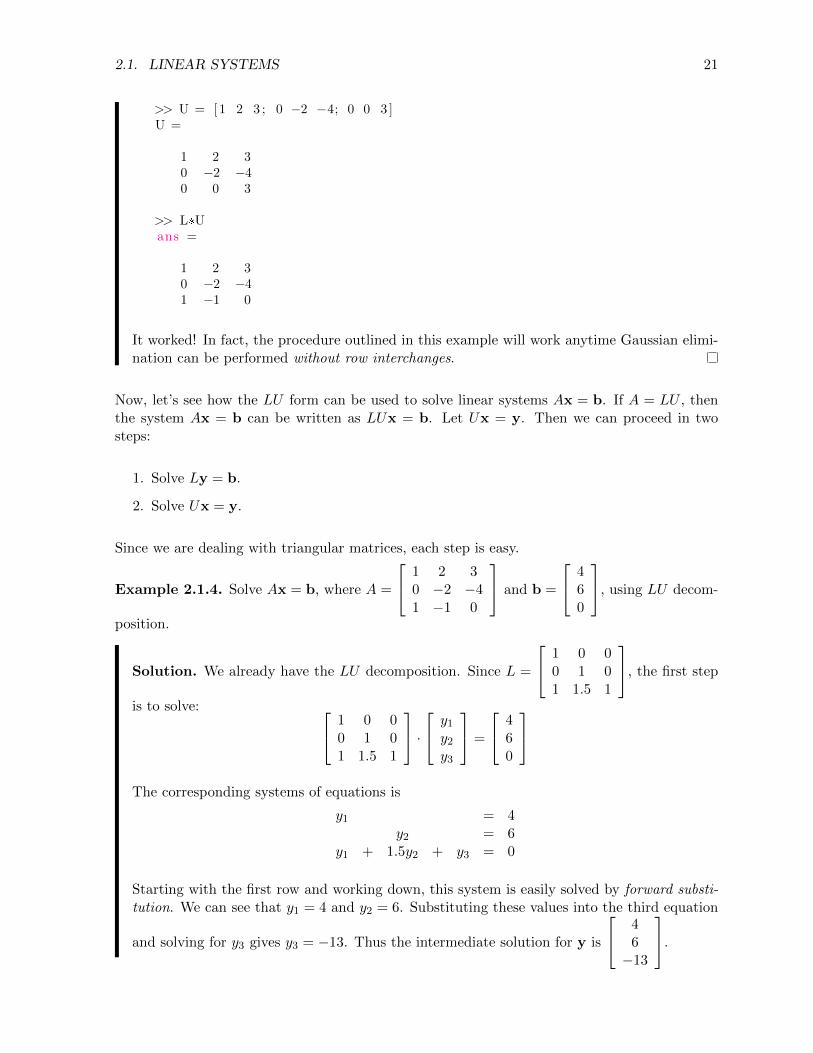
>> U = [ 1 2 3 ; 0 −2 −4; 0 0 3 ]U =
1 2 30 −2 −40 0 3
>> L*Uans =
1 2 30 −2 −41 −1 0
It worked! In fact, the procedure outlined in this example will work anytime Gaussian elimi-nation can be performed without row interchanges.
Now, let’s see how the LU form can be used to solve linear systems Ax = b. If A = LU , thenthe system Ax = b can be written as LUx = b. Let Ux = y. Then we can proceed in twosteps:
1. Solve Ly = b.
2. Solve Ux = y.
Since we are dealing with triangular matrices, each step is easy.
Example 2.1.4. Solve Ax = b, where A =
1 2 30 −2 −41 −1 0
and b =
460
, using LU decom-
position.
Solution. We already have the LU decomposition. Since L =
1 0 00 1 01 1.5 1
, the first step
is to solve: 1 0 00 1 01 1.5 1
· y1y2y3
=
460
The corresponding systems of equations is
y1 = 4y2 = 6
y1 + 1.5y2 + y3 = 0
Starting with the first row and working down, this system is easily solved by forward substi-tution. We can see that y1 = 4 and y2 = 6. Substituting these values into the third equation
and solving for y3 gives y3 = −13. Thus the intermediate solution for y is
46−13
.
22 CHAPTER 2. MATRICES AND LINEAR SYSTEMS
Step two is to solve Ux = y, which looks like: 1 2 30 −2 −40 0 3
· x1x2x3
=
46−13
This is easily solved by backward substitution to get x =
17/317/3−13/3
.
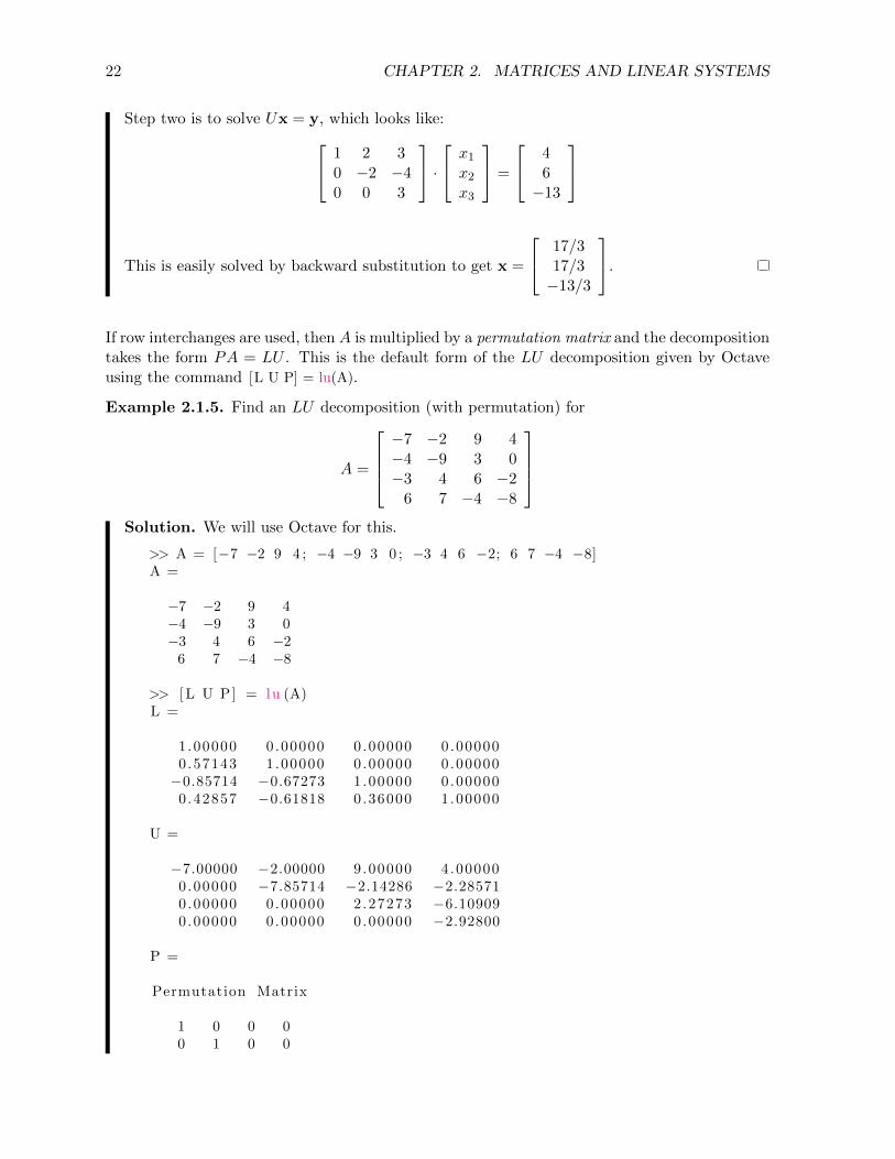
If row interchanges are used, then A is multiplied by a permutation matrix and the decompositiontakes the form PA = LU . This is the default form of the LU decomposition given by Octaveusing the command [L U P] = lu(A).
Example 2.1.5. Find an LU decomposition (with permutation) for
A =
−7 −2 9 4−4 −9 3 0−3 4 6 −2
6 7 −4 −8
Solution. We will use Octave for this.
>> A = [−7 −2 9 4 ; −4 −9 3 0 ; −3 4 6 −2; 6 7 −4 −8]A =
−7 −2 9 4−4 −9 3 0−3 4 6 −2
6 7 −4 −8
>> [ L U P] = lu (A)L =
1.00000 0.00000 0.00000 0.000000.57143 1.00000 0.00000 0.00000−0.85714 −0.67273 1.00000 0.00000
0.42857 −0.61818 0.36000 1.00000
U =
−7.00000 −2.00000 9.00000 4.000000.00000 −7.85714 −2.14286 −2.285710.00000 0.00000 2.27273 −6.109090.00000 0.00000 0.00000 −2.92800
P =
Permutation Matrix
1 0 0 00 1 0 0
2.2. POLYNOMIAL CURVE FITTING 23
0 0 0 10 0 1 0
Refer to Exercise 4 to see how PA = LU can be used to solve a linear system, using a methodalmost to identical to what we did in Example 2.1.4.
LU decomposition is widely used in numerical linear algebra. In fact, it is the basis of howOctave’s left division operation works. It is especially efficient to use LU decomposition whenone is solving several systems of equations that all have the same coefficient matrix, but differentright side constants. The LU decomposition only needs to be done once for all of the systemswith that coefficient matrix.
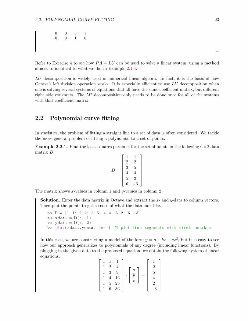
2.2 Polynomial curve fitting
In statistics, the problem of fitting a straight line to a set of data is often considered. We tacklethe more general problem of fitting a polynomial to a set of points.
Example 2.2.1. Find the least-squares parabola for the set of points in the following 6×2 datamatrix D.
D =
1 12 23 54 45 26 −3
The matrix shows x-values in column 1 and y-values in column 2.
Solution. Enter the data matrix in Octave and extract the x- and y-data to column vectors.Then plot the points to get a sense of what the data look like.
>> D = [ 1 1 ; 2 2 ; 3 5 ; 4 4 ; 5 2 ; 6 −3]>> xdata = D( : , 1)>> ydata = D( : , 2)>> p lo t ( xdata , ydata , 'o− ' ) % p lo t l i n e segments with c i r c l e markers
In this case, we are constructing a model of the form y = a + bx + cx2, but it is easy to seehow our approach generalizes to polynomials of any degree (including linear functions). Byplugging in the given data to the proposed equation, we obtain the following system of linearequations.
1 1 11 2 41 3 91 4 161 5 251 6 36
· abc
=
12542−3
24 CHAPTER 2. MATRICES AND LINEAR SYSTEMS
Notice the form of the coefficient matrix, which we’ll call A. The first column is all ones, thesecond column is the x-values, and the third column is the square of the x-values (this columnwould not appear if we were using a linear model). The right-side constants are the y-values.There are several ways to construct the coefficient matrix in Octave. One approach is to usethe ones command to create a matrix of ones of the appropriate size, and then overwrite thesecond and third columns with the correct data.
>> A = ones (6 , 3) ;>> A( : , 2) = xdata ;>> A( : , 3) = xdata .ˆ2A =
1 1 11 2 41 3 91 4 161 5 251 6 36
Note the use of elementwise exponentiation to square each value of the vector xdata. Oursystem is inconsistent. It can be shown that the least-squares solution comes from solving
the normal equations, ATAb = ATy, where b is the vector
abc
of polynomial coefficients.
We can use Octave to construct the normal equations.
>> A' *Aans =
6 21 9121 91 44191 441 2275
>> A' * ydataans =
112860
The corresponding augmented matrix is: 6 21 91 1121 91 441 2891 441 2275 60
We can then solve the problem using Gaussian elimination. Here is one way to create theaugmented matrix and row-reduce it:
>> B = A' *A;>> B( : , 4) = A' * ydata ;
2.2. POLYNOMIAL CURVE FITTING 25
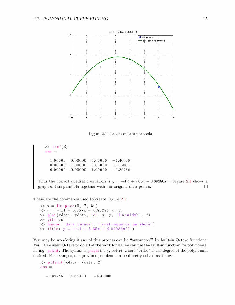
Figure 2.1: Least-squares parabola
>> r r e f (B)ans =
1.00000 0.00000 0.00000 −4.400000.00000 1.00000 0.00000 5.650000.00000 0.00000 1.00000 −0.89286
Thus the correct quadratic equation is y = −4.4 + 5.65x − 0.89286x2. Figure 2.1 shows agraph of this parabola together with our original data points.
These are the commands used to create Figure 2.1:
>> x = l i n s p a c e (0 , 7 , 50) ;>> y = −4.4 + 5.65*x − 0.89286*x . ˆ 2 ;>> p lo t ( xdata , ydata , ' o ' , x , y , ' l i n ew id th ' , 2)>> g r id on ;>> l egend ( ' data va lue s ' , ' l e a s t−squares parabola ' )>> t i t l e ( 'y = −4.4 + 5.65 x − 0.89286 xˆ2 ' )
You may be wondering if any of this process can be “automated” by built-in Octave functions.Yes! If we want Octave to do all of the work for us, we can use the built-in function for polynomialfitting, polyfit . The syntax is polyfit (x, y, order), where “order” is the degree of the polynomialdesired. For example, our previous problem can be directly solved as follows.
>> p o l y f i t ( xdata , ydata , 2)ans =
−0.89286 5.65000 −4.40000
26 CHAPTER 2. MATRICES AND LINEAR SYSTEMS
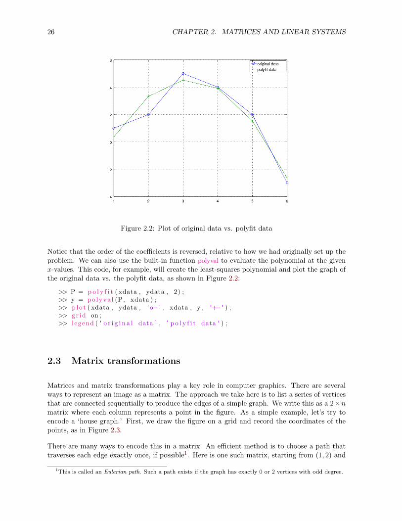
Figure 2.2: Plot of original data vs. polyfit data
Notice that the order of the coefficients is reversed, relative to how we had originally set up theproblem. We can also use the built-in function polyval to evaluate the polynomial at the givenx-values. This code, for example, will create the least-squares polynomial and plot the graph ofthe original data vs. the polyfit data, as shown in Figure 2.2:
>> P = p o l y f i t ( xdata , ydata , 2) ;>> y = po lyva l (P, xdata ) ;>> p lo t ( xdata , ydata , 'o− ' , xdata , y , '+− ' ) ;>> g r id on ;>> l egend ( ' o r i g i n a l data ' , ' p o l y f i t data ' ) ;
2.3 Matrix transformations
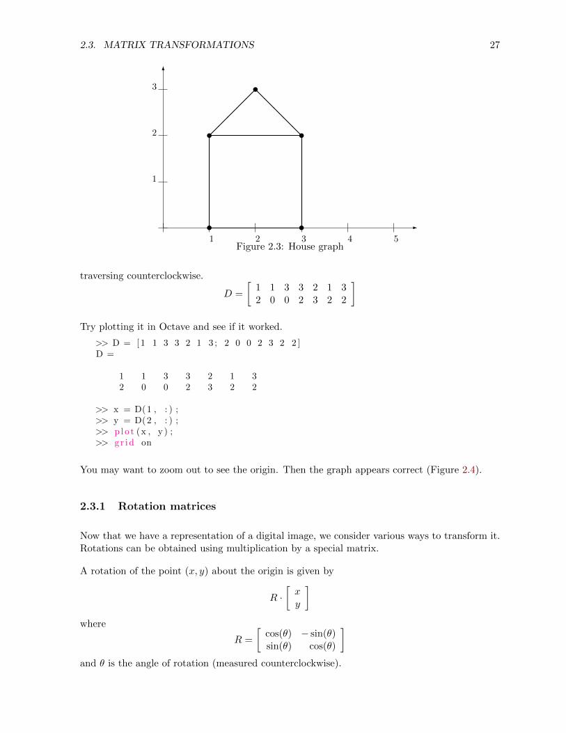
Matrices and matrix transformations play a key role in computer graphics. There are severalways to represent an image as a matrix. The approach we take here is to list a series of verticesthat are connected sequentially to produce the edges of a simple graph. We write this as a 2×nmatrix where each column represents a point in the figure. As a simple example, let’s try toencode a ‘house graph.’ First, we draw the figure on a grid and record the coordinates of thepoints, as in Figure 2.3.
There are many ways to encode this in a matrix. An efficient method is to choose a path thattraverses each edge exactly once, if possible1. Here is one such matrix, starting from (1, 2) and
1This is called an Eulerian path. Such a path exists if the graph has exactly 0 or 2 vertices with odd degree.
2.3. MATRIX TRANSFORMATIONS 27
-
6
t t
tt
t�����@
@@@@
1 2 3 4 5
1
2
3
Figure 2.3: House graph
traversing counterclockwise.
D =
[1 1 3 3 2 1 32 0 0 2 3 2 2
]
Try plotting it in Octave and see if it worked.
>> D = [ 1 1 3 3 2 1 3 ; 2 0 0 2 3 2 2 ]D =
1 1 3 3 2 1 32 0 0 2 3 2 2
>> x = D(1 , : ) ;>> y = D(2 , : ) ;>> p lo t (x , y ) ;>> g r id on
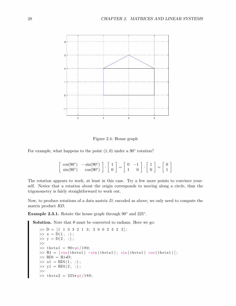
You may want to zoom out to see the origin. Then the graph appears correct (Figure 2.4).
2.3.1 Rotation matrices
Now that we have a representation of a digital image, we consider various ways to transform it.Rotations can be obtained using multiplication by a special matrix.
A rotation of the point (x, y) about the origin is given by
R ·[xy
]where
R =
[cos(θ) − sin(θ)sin(θ) cos(θ)
]and θ is the angle of rotation (measured counterclockwise).
28 CHAPTER 2. MATRICES AND LINEAR SYSTEMS
Figure 2.4: House graph
For example, what happens to the point (1, 0) under a 90◦ rotation?
[cos(90◦) − sin(90◦)sin(90◦) cos(90◦)
]·[
10
]=
[0 −11 0
]·[
10
]=
[01
]
The rotation appears to work, at least in this case. Try a few more points to convince your-self. Notice that a rotation about the origin corresponds to moving along a circle, thus thetrigonometry is fairly straightforward to work out.
Now, to produce rotations of a data matrix D, encoded as above, we only need to compute thematrix product RD.
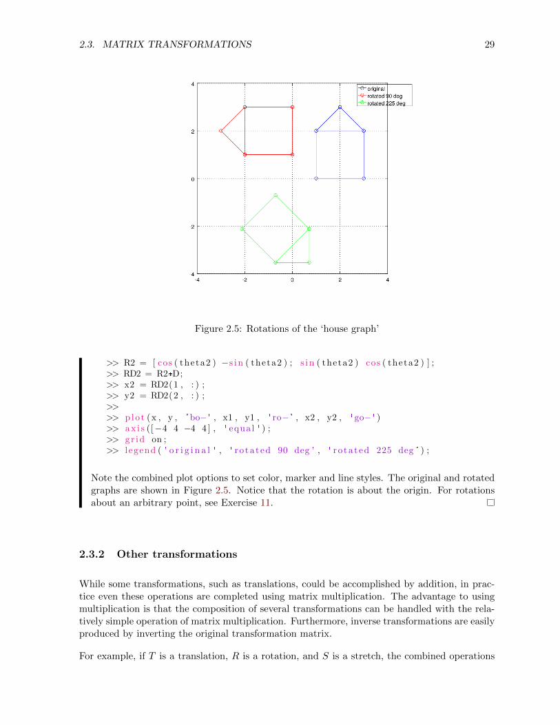
Example 2.3.1. Rotate the house graph through 90◦ and 225◦.
Solution. Note that θ must be converted to radians. Here we go:
>> D = [ 1 1 3 3 2 1 3 ; 2 0 0 2 3 2 2 ] ;>> x = D(1 , : ) ;>> y = D(2 , : ) ;>>>> theta1 = 90* pi /180 ;>> R1 = [ cos ( theta1 ) −s i n ( theta1 ) ; s i n ( theta1 ) cos ( theta1 ) ] ;>> RD1 = R1*D;>> x1 = RD1(1 , : ) ;>> y1 = RD1(2 , : ) ;>>>> theta2 = 225* pi /180 ;
2.3. MATRIX TRANSFORMATIONS 29
Figure 2.5: Rotations of the ‘house graph’
>> R2 = [ cos ( theta2 ) −s i n ( theta2 ) ; s i n ( theta2 ) cos ( theta2 ) ] ;>> RD2 = R2*D;>> x2 = RD2(1 , : ) ;>> y2 = RD2(2 , : ) ;>>>> p lo t (x , y , 'bo− ' , x1 , y1 , ' ro− ' , x2 , y2 , ' go− ' )>> a x i s ([−4 4 −4 4 ] , ' equal ' ) ;>> g r id on ;>> l egend ( ' o r i g i n a l ' , ' ro ta ted 90 deg ' , ' ro ta ted 225 deg ' ) ;
Note the combined plot options to set color, marker and line styles. The original and rotatedgraphs are shown in Figure 2.5. Notice that the rotation is about the origin. For rotationsabout an arbitrary point, see Exercise 11.
2.3.2 Other transformations
While some transformations, such as translations, could be accomplished by addition, in prac-tice even these operations are completed using matrix multiplication. The advantage to usingmultiplication is that the composition of several transformations can be handled with the rela-tively simple operation of matrix multiplication. Furthermore, inverse transformations are easilyproduced by inverting the original transformation matrix.
For example, if T is a translation, R is a rotation, and S is a stretch, the combined operations
30 CHAPTER 2. MATRICES AND LINEAR SYSTEMS
of first translating, then rotating, then stretching can be completed with the matrix SRT anda data matrix D can be transformed with the product (SRT )D. The inverse of these combinedoperations is (SRT )−1 = T−1R−1S−1.
Refer to Exercises 10–11 for some of the details and an example.
EXERCISES 31
Chapter 2 Exercises
1. Solve the system of equations using Gaussian elimination row operations−x1 + x2 − 2x3 = 1x1 + x2 + 2x3 = −1x1 + 3x2 + 2x3 = −11
To document your work in Octave, click “select all,” then “copy” under the edit menu,and paste your work into a Word or text document. After you have the row-echelon form,solve the system by hand on paper, using backward substitution.
2. Use the Gaussian elimination multipliers from Exercise 1 to write an LU decomposition
for A =
−1 1 −21 1 21 3 2
. Use this factorization to solve the system from Exercise 1.
3. Let A =
1 −3 52 −4 30 1 −1
be the coefficient matrix for a system of linear equations Ax = b,
where b = 〈1,−1, 3〉. Solve the system using left division. Then, construct an augmentedmatrix A1 and use rref to row-reduce it. Compare the results.
4. Use LU decomposition to solve the system from Exercise 3. Use Octave’s [L U P] = lu(A)
command. To use PA = LU to solve Ax = b, first multiply through by P , then replacePA with LU :
Ax = bPAx = PbLUx = Pb
First solve Ly = Pb, then solve Ux = y.
5. So far we have only looked at consistent systems. How does Octave handle inconsistentsystems? Let’s turn our previous system into an inconsistent one. Let Ax = b be thesystem from Exercise 3. To make this into a inconsistent system, we will make one row ofthe coefficient matrix into a linear combination of some other rows, without making thecorresponding adjustment to the right-side constants. Do the following:
>> A(1 , : ) = 3*A(2 , : ) − 4*A(3 , : )
Now Ax = b should be an inconsistent system. Try solving it and see what Octave does.Compare the results of left-division with the row-reduced echelon form. How can you seethat the system is inconsistent?
6. Octave can easily solve large problems that we would never consider working by-hand.Let’s try constructing and solving a larger systems of equations. The command rand(m, n)
will generate an m× n matrix with entries uniformly distributed from the interval (0, 1).If we want integer entries, we can multiply by 10 and use the floor function to chop offthe decimal. Use this command to generate an augmented matrix M for a system of 25equations in 25 unknowns:
32 CHAPTER 2. MATRICES AND LINEAR SYSTEMS
>> M = f l o o r (10* rand (25 , 26) ) ;
Note the semicolon. This suppresses the output to the screen, since the matrix is now toolarge to display conveniently. Solve the system of equations using rref and/or left divisionand save the solution as a column vector x.
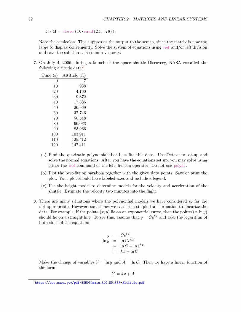
7. On July 4, 2006, during a launch of the space shuttle Discovery, NASA recorded thefollowing altitude data2.
Time (s) Altitude (ft)
0 710 93820 4,16030 9,87240 17,63550 26,96960 37,74670 50,54880 66,03390 83,966
100 103,911110 125,512120 147,411
(a) Find the quadratic polynomial that best fits this data. Use Octave to set-up andsolve the normal equations. After you have the equations set up, you may solve usingeither the rref command or the left-division operator. Do not use polyfit .
(b) Plot the best-fitting parabola together with the given data points. Save or print theplot. Your plot should have labeled axes and include a legend.
(c) Use the height model to determine models for the velocity and acceleration of theshuttle. Estimate the velocity two minutes into the flight.
8. There are many situations where the polynomial models we have considered so far arenot appropriate. However, sometimes we can use a simple transformation to linearize thedata. For example, if the points (x, y) lie on an exponential curve, then the points (x, ln y)should lie on a straight line. To see this, assume that y = Cekx and take the logarithm ofboth sides of the equation:
y = Cekx
ln y = lnCekx
= lnC + ln ekx
= kx+ lnC
Make the change of variables Y = ln y and A = lnC. Then we have a linear function ofthe form
Y = kx+A
2https://www.nasa.gov/pdf/585034main_ALG_ED_SSA-Altitude.pdf
EXERCISES 33
We can find the line that best fits the (x, Y )-data and then use inverse transformations toobtain the exponential model we need:
y = Cekx
whereC = eA
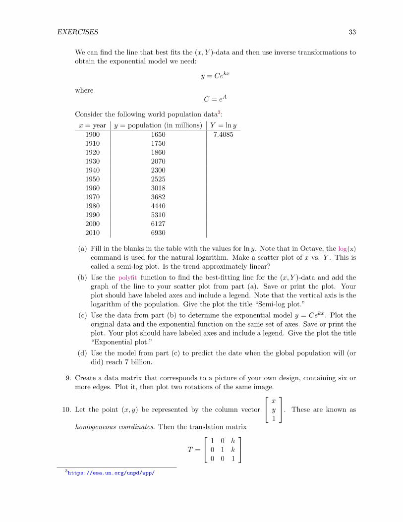
Consider the following world population data3:
x = year y = population (in millions) Y = ln y
1900 1650 7.40851910 17501920 18601930 20701940 23001950 25251960 30181970 36821980 44401990 53102000 61272010 6930
(a) Fill in the blanks in the table with the values for ln y. Note that in Octave, the log(x)
command is used for the natural logarithm. Make a scatter plot of x vs. Y . This iscalled a semi-log plot. Is the trend approximately linear?
(b) Use the polyfit function to find the best-fitting line for the (x, Y )-data and add thegraph of the line to your scatter plot from part (a). Save or print the plot. Yourplot should have labeled axes and include a legend. Note that the vertical axis is thelogarithm of the population. Give the plot the title “Semi-log plot.”
(c) Use the data from part (b) to determine the exponential model y = Cekx. Plot theoriginal data and the exponential function on the same set of axes. Save or print theplot. Your plot should have labeled axes and include a legend. Give the plot the title“Exponential plot.”
(d) Use the model from part (c) to predict the date when the global population will (ordid) reach 7 billion.
9. Create a data matrix that corresponds to a picture of your own design, containing six ormore edges. Plot it, then plot two rotations of the same image.
10. Let the point (x, y) be represented by the column vector
xy1
. These are known as
homogeneous coordinates. Then the translation matrix
T =
1 0 h0 1 k0 0 1
3https://esa.un.org/unpd/wpp/
34 CHAPTER 2. MATRICES AND LINEAR SYSTEMS
is used to move the point (x, y) to (x+ h, y + k) as follows: 1 0 h0 1 k0 0 1
· xy1
=
x+ hy + k
1
Use a translation matrix and homogeneous coordinates to shift the graph you created inproblem 9 as follows: shift 3 units left and 2 units up.
11. The translation method described in problem 10 can be combined with a rotation matrixto give rotations around an arbitrary point. Suppose for example that we wished to rotatethe house graph from Figure 2.3 about the center of the rectangular portion (coordinates(2, 1) in the original figure). This can be done by using homogeneous coordinates and atranslation T to move the figure, then a rotation matrix R for the rotation. The form ofR is now
R =
cos(θ) − sin(θ) 0sin(θ) cos(θ) 0
0 0 1
The shifted and rotated figure is then given by (RT )D. To shift back to the originalposition, an inverse transformation T−1 is used. Thus the rotated image can be found bycomputing (T−1RT )D. Use this method to rotate the house graph 90◦ about the point(1, 2). Show the combined transformation matrix T−1RT and the results.
Chapter 3
Calculus
3.1 Limits, sequences, and series
Octave is an excellent tool for many types of numerical experiments. Octave is a full-fledgedprogramming language supporting many types of loops and conditional statements. However,since it is a vector-based language, many things that would be done using loops in FORTRANor other languages can be “vectorized.” As an example, let’s construct some numerical evidenceto guess at the value of the following limit:
limn→∞
(1 +
1
n
)n
We simply want to evaluate the expression for a series of larger and larger n-values. This iswhat we mean by vectorized code: instead of writing a loop to evaluate the function multipletimes, we will generate a vector of input values, then evaluate the function using the vectorinput. This produces code that is easier to read and understand, and executes faster, due toOctave’s underlying efficient algorithms for matrix operations.
First, we need to define the function. There are a number of ways to do this. The method weuse here is known as an anonymous function. This is a good way to quickly define a simplefunction.
>> f = @(n) (1 + 1 ./ n) . ˆ n ; % anonymous func t i on
Note the use of elementwise operations. We have named the function f . The input variable isdesignated by the @-sign followed by the variable in parentheses. The expression that followsgives the rule to be used when the function is evaluated. Now f can be used like any functionin Octave.
Next we create an index variable, consisting of the integers from 0 to 9:
>> k = [ 0 : 1 : 9 ] ' % index v a r i a b l ek =
35
36 CHAPTER 3. CALCULUS
0123456789
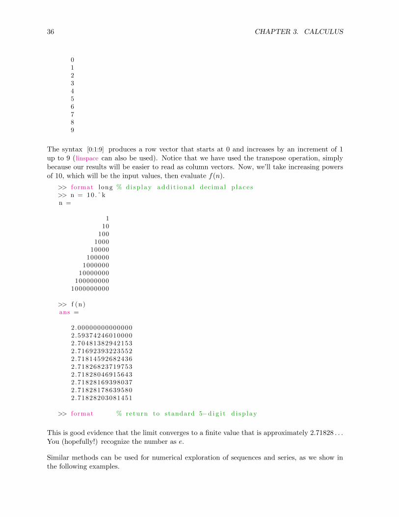
The syntax [0:1:9] produces a row vector that starts at 0 and increases by an increment of 1up to 9 (linspace can also be used). Notice that we have used the transpose operation, simplybecause our results will be easier to read as column vectors. Now, we’ll take increasing powersof 10, which will be the input values, then evaluate f(n).
>> format long % d i s p l a y a d d i t i o n a l decimal p l a c e s>> n = 10 .ˆ kn =
110
1001000
10000100000
100000010000000
1000000001000000000
>> f (n )ans =
2.000000000000002.593742460100002.704813829421532.716923932235522.718145926824362.718268237197532.718280469156432.718281693980372.718281786395802.71828203081451
>> format % return to standard 5−d i g i t d i s p l ay
This is good evidence that the limit converges to a finite value that is approximately 2.71828 . . .You (hopefully!) recognize the number as e.
Similar methods can be used for numerical exploration of sequences and series, as we show inthe following examples.
3.1. LIMITS, SEQUENCES, AND SERIES 37
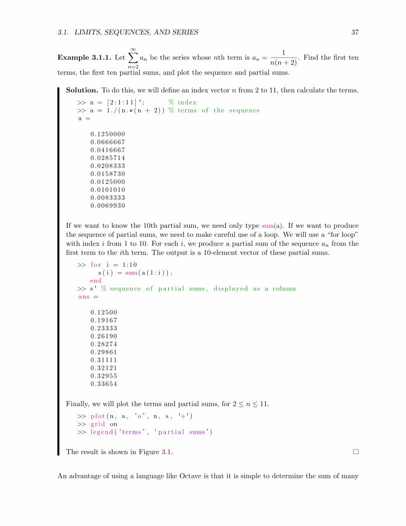
Example 3.1.1. Let
∞∑n=2
an be the series whose nth term is an =1
n(n+ 2). Find the first ten
terms, the first ten partial sums, and plot the sequence and partial sums.
Solution. To do this, we will define an index vector n from 2 to 11, then calculate the terms.
>> n = [ 2 : 1 : 1 1 ] ' ; % index>> a = 1 . / ( n . * ( n + 2) ) % terms o f the sequencea =
0.12500000.06666670.04166670.02857140.02083330.01587300.01250000.01010100.00833330.0069930
If we want to know the 10th partial sum, we need only type sum(a). If we want to producethe sequence of partial sums, we need to make careful use of a loop. We will use a “for loop”with index i from 1 to 10. For each i, we produce a partial sum of the sequence an from thefirst term to the ith term. The output is a 10-element vector of these partial sums.
>> f o r i = 1 :10s ( i ) = sum( a ( 1 : i ) ) ;
end>> s ' % sequence o f p a r t i a l sums , d i sp layed as a columnans =
0.125000.191670.233330.261900.282740.298610.311110.321210.329550.33654
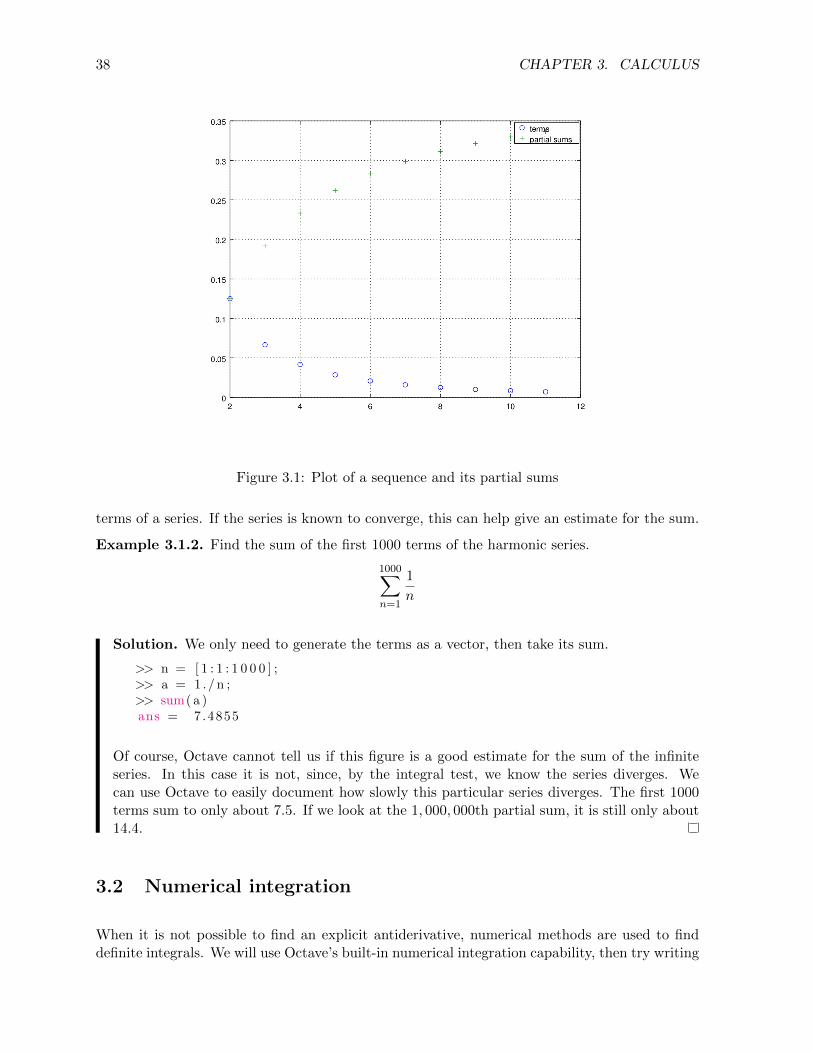
Finally, we will plot the terms and partial sums, for 2 ≤ n ≤ 11.
>> p lo t (n , a , ' o ' , n , s , '+ ' )>> g r id on>> l egend ( ' terms ' , ' p a r t i a l sums ' )
The result is shown in Figure 3.1.
An advantage of using a language like Octave is that it is simple to determine the sum of many
38 CHAPTER 3. CALCULUS
Figure 3.1: Plot of a sequence and its partial sums
terms of a series. If the series is known to converge, this can help give an estimate for the sum.
Example 3.1.2. Find the sum of the first 1000 terms of the harmonic series.
1000∑n=1
1
n
Solution. We only need to generate the terms as a vector, then take its sum.
>> n = [ 1 : 1 : 1 0 0 0 ] ;>> a = 1 ./ n ;>> sum( a )ans = 7.4855
Of course, Octave cannot tell us if this figure is a good estimate for the sum of the infiniteseries. In this case it is not, since, by the integral test, we know the series diverges. Wecan use Octave to easily document how slowly this particular series diverges. The first 1000terms sum to only about 7.5. If we look at the 1, 000, 000th partial sum, it is still only about14.4.
3.2 Numerical integration
When it is not possible to find an explicit antiderivative, numerical methods are used to finddefinite integrals. We will use Octave’s built-in numerical integration capability, then try writing
3.2. NUMERICAL INTEGRATION 39
our own scripts to apply the midpoint rule, trapezoid rule, and Simpson’s rule.
3.2.1 Quadrature
Octave has several built in functions to calculate definite integrals. We will use the quad com-mand. ‘Quad’ is short for quadrature, which refers to the process of numeric integration.
Example 3.2.1. Estimate
∫ π/2
0ex
2cos(x) dx using Octave’s quad algorithm.
Solution. The correct syntax is quad('f ' , a, b). We need to first define the function.
>> f unc t i on y = f ( x )y = exp ( x . ˆ 2 ) .* cos ( x ) ;
end>> quad ( ' f ' , 0 , p i /2)ans = 1.8757
Note that the function exp(x) is used for ex. In this example, we used the function . . . end
construction to define f . This is a versatile format that allows for multiple operations andoutputs. We could have also used an anonymous function. Note that no quotes are usedaround f if using an anonymous function.
3.2.2 Approximating sums
The midpoint rule, trapezoid rule, and Simpson’s rule are common algorithms used for numericalintegration. Ideally these are implemented in a computer program and Octave is well suited forthis purpose.
Let {a = x0, x1, x2, . . . , xn = b} be a partition of [a, b] into n subintervals, each of width
∆x =b− an
. Then
∫ b
af(x) dx can be approximated as follows.
Midpoint rule:∆x [f(m1) + f(m2) + · · ·+ f(mn)]
where mi is the midpoint of the ith subinterval.
Trapezoid rule:
∆x
2[f(x0) + 2f(x1) + 2f(x2) + · · ·+ 2f(xn−1) + 2f(xn)]
where xi = a+ i∆x.
Simpson’s rule:
∆x
3[f(x0) + 4f(x1) + 2f(x2) + 4f(x3) + · · ·+ 2f(xn−2) + 4f(xn−1) + f(xn)]
where xi = a+ i∆x.
40 CHAPTER 3. CALCULUS
Notice that the sum in the midpoint formula has n terms, while the trapezoid and Simpson’srules have n+1 (the index i goes from 0 to n). To implement these rules in Octave, we will writescript files, which are plain text files containing a series of Octave commands. Use a text editor,such as Notepad, Notepad++, or Emacs. A script file needs to have a “.m” extension (not the.txt used by default in Windows for text files) and cannot begin with the keyword function. TheOctave GUI has its own built in text editor which can be accessed by changing to the “Editor”tab option displayed below the main command window. This editor is ideal for creating, editing,and running .m files and will automatically color code comments and key words.
Example 3.2.2. Write an Octave script to calculate a midpoint rule approximation of∫ π/2
0ex
2cos(x) dx
using n = 100.
Solution. The basic strategy is to use a loop that adds an additional function value to arunning total with each iteration. Then the final answer is found by multiplying the sum by∆x.
The following code can be used. Enter the code in a plain text file and name it “midpoint.m”.It must be placed in your working directory, then it can be run by typing ‘midpoint’ at thecommand prompt.
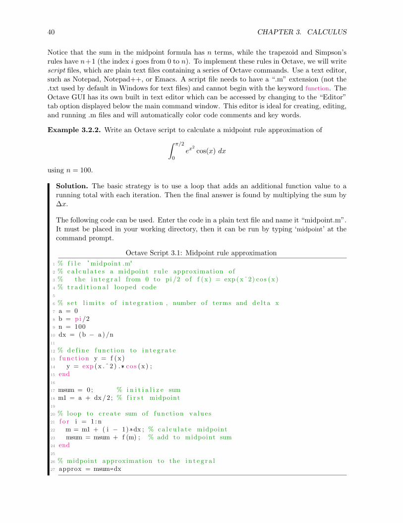
Octave Script 3.1: Midpoint rule approximation
1 % f i l e ' midpoint .m'
2 % c a l c u l a t e s a midpoint r u l e approximation o f3 % the i n t e g r a l from 0 to p i /2 o f f ( x ) = exp ( xˆ2) cos ( x )4 % t r a d i t i o n a l looped code5
6 % s e t l i m i t s o f i n t e g r a t i o n , number o f terms and d e l t a x7 a = 08 b = pi /29 n = 100
10 dx = (b − a ) /n11
12 % d e f i n e func t i on to i n t e g r a t e13 f unc t i on y = f ( x )14 y = exp ( x . ˆ 2 ) .* cos ( x ) ;15 end16
17 msum = 0 ; % i n i t i a l i z e sum18 m1 = a + dx /2 ; % f i r s t midpoint19
20 % loop to c r e a t e sum of func t i on va lue s21 f o r i = 1 : n22 m = m1 + ( i − 1) *dx ; % c a l c u l a t e midpoint23 msum = msum + f (m) ; % add to midpoint sum24 end25
26 % midpoint approximation to the i n t e g r a l27 approx = msum*dx
3.2. NUMERICAL INTEGRATION 41
Now run midpoint.m.
>> midpointa = 0b = 1.5708n = 100dx = 0.015708approx = 1.8758
The traditional code works fine, but because Octave is a vector-based language, it is also possibleto write vectorized code that does not require any loops.
Example 3.2.3. Write a vectorized Octave script to calculate a midpoint rule approximationof ∫ π/2
0ex
2cos(x) dx
using n = 100.
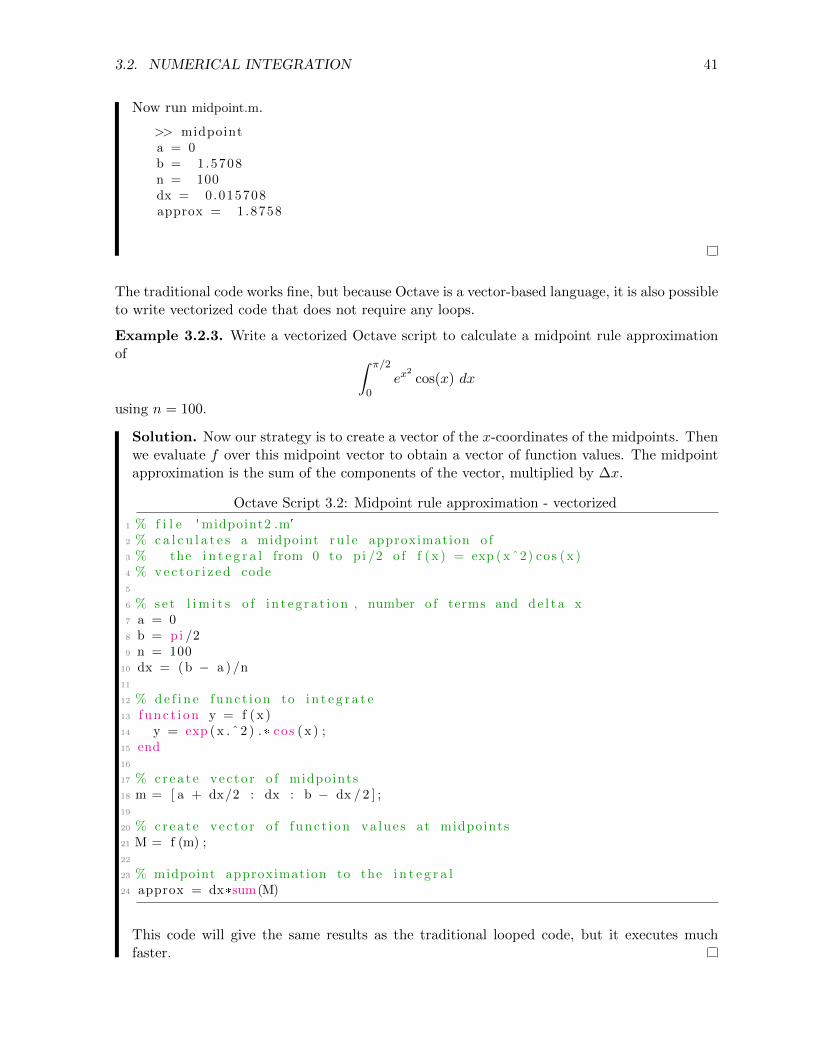
Solution. Now our strategy is to create a vector of the x-coordinates of the midpoints. Thenwe evaluate f over this midpoint vector to obtain a vector of function values. The midpointapproximation is the sum of the components of the vector, multiplied by ∆x.
Octave Script 3.2: Midpoint rule approximation - vectorized
1 % f i l e ' midpoint2 .m'
2 % c a l c u l a t e s a midpoint r u l e approximation o f3 % the i n t e g r a l from 0 to p i /2 o f f ( x ) = exp ( xˆ2) cos ( x )4 % v e c t o r i z e d code5
6 % s e t l i m i t s o f i n t e g r a t i o n , number o f terms and d e l t a x7 a = 08 b = pi /29 n = 100
10 dx = (b − a ) /n11
12 % d e f i n e func t i on to i n t e g r a t e13 f unc t i on y = f ( x )14 y = exp ( x . ˆ 2 ) .* cos ( x ) ;15 end16
17 % c r e a t e vec to r o f midpoints18 m = [ a + dx/2 : dx : b − dx / 2 ] ;19
20 % c r e a t e vec to r o f func t i on va lue s at midpoints21 M = f (m) ;22
23 % midpoint approximation to the i n t e g r a l24 approx = dx*sum(M)
This code will give the same results as the traditional looped code, but it executes muchfaster.
42 CHAPTER 3. CALCULUS
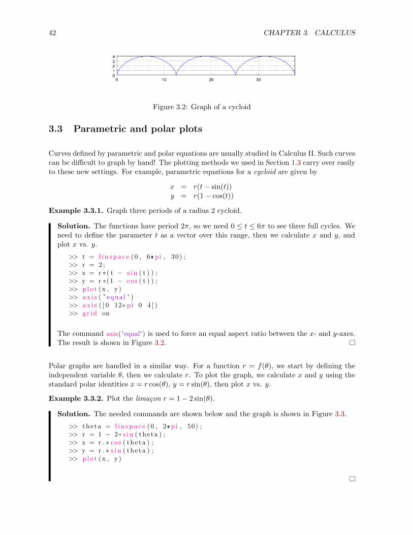
Figure 3.2: Graph of a cycloid
3.3 Parametric and polar plots
Curves defined by parametric and polar equations are usually studied in Calculus II. Such curvescan be difficult to graph by hand! The plotting methods we used in Section 1.3 carry over easilyto these new settings. For example, parametric equations for a cycloid are given by
x = r(t− sin(t))y = r(1− cos(t))
Example 3.3.1. Graph three periods of a radius 2 cycloid.
Solution. The functions have period 2π, so we need 0 ≤ t ≤ 6π to see three full cycles. Weneed to define the parameter t as a vector over this range, then we calculate x and y, andplot x vs. y.
>> t = l i n s p a c e (0 , 6*pi , 30) ;>> r = 2 ;>> x = r *( t − s i n ( t ) ) ;>> y = r *(1 − cos ( t ) ) ;>> p lo t (x , y )>> a x i s ( ' equal ' )>> a x i s ( [ 0 12* pi 0 4 ] )>> g r id on
The command axis( 'equal') is used to force an equal aspect ratio between the x- and y-axes.The result is shown in Figure 3.2.
Polar graphs are handled in a similar way. For a function r = f(θ), we start by defining theindependent variable θ, then we calculate r. To plot the graph, we calculate x and y using thestandard polar identities x = r cos(θ), y = r sin(θ), then plot x vs. y.
Example 3.3.2. Plot the limacon r = 1− 2 sin(θ).
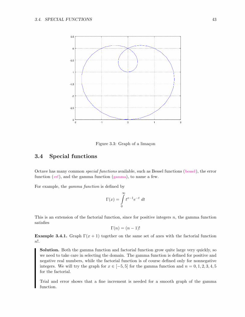
Solution. The needed commands are shown below and the graph is shown in Figure 3.3.
>> theta = l i n s p a c e (0 , 2*pi , 50) ;>> r = 1 − 2* s i n ( theta ) ;>> x = r .* cos ( theta ) ;>> y = r .* s i n ( theta ) ;>> p lo t (x , y )
3.4. SPECIAL FUNCTIONS 43
Figure 3.3: Graph of a limacon
3.4 Special functions
Octave has many common special functions available, such as Bessel functions (bessel), the errorfunction (erf), and the gamma function (gamma), to name a few.
For example, the gamma function is defined by
Γ(x) =
∞∫0
tx−1e−t dt
This is an extension of the factorial function, since for positive integers n, the gamma functionsatisfies
Γ(n) = (n− 1)!
Example 3.4.1. Graph Γ(x + 1) together on the same set of axes with the factorial functionn!.
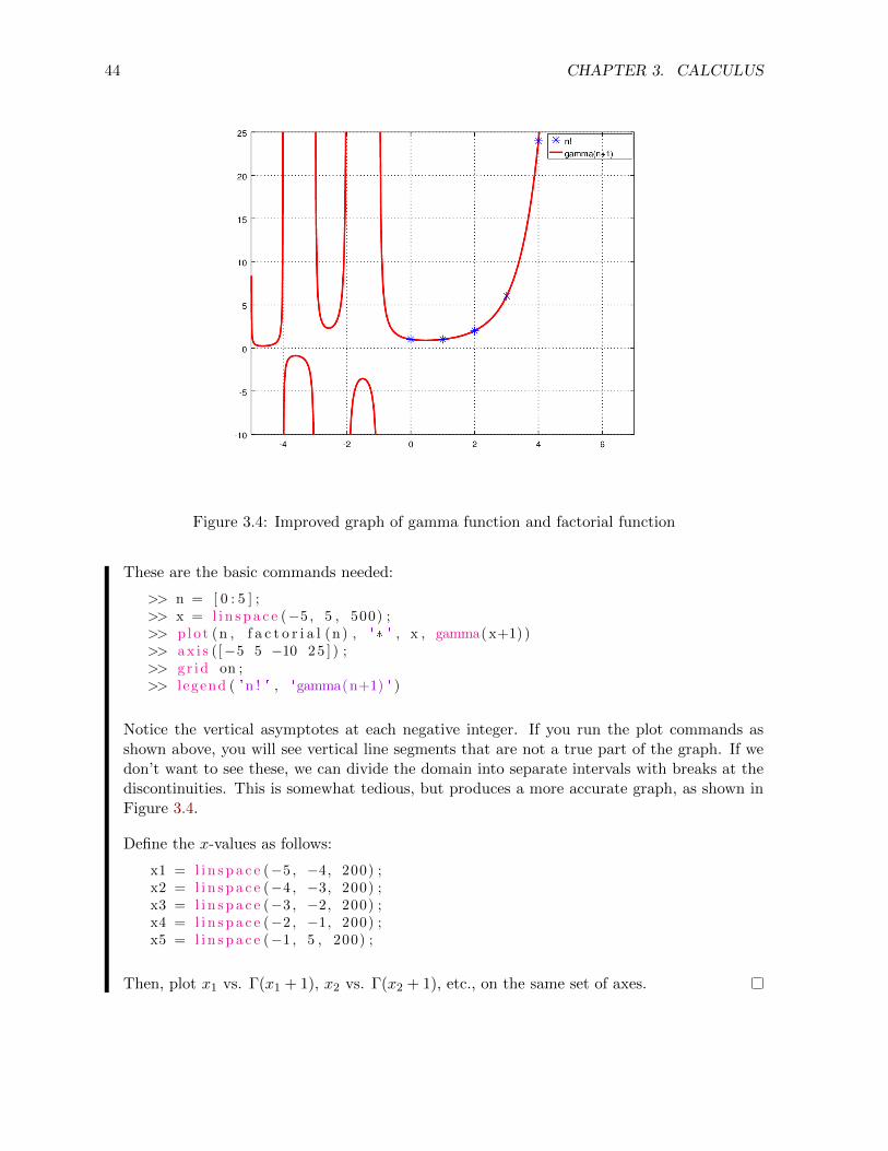
Solution. Both the gamma function and factorial function grow quite large very quickly, sowe need to take care in selecting the domain. The gamma function is defined for positive andnegative real numbers, while the factorial function is of course defined only for nonnegativeintegers. We will try the graph for x ∈ [−5, 5] for the gamma function and n = 0, 1, 2, 3, 4, 5for the factorial.
Trial and error shows that a fine increment is needed for a smooth graph of the gammafunction.
44 CHAPTER 3. CALCULUS
Figure 3.4: Improved graph of gamma function and factorial function
These are the basic commands needed:
>> n = [ 0 : 5 ] ;>> x = l i n s p a c e (−5 , 5 , 500) ;>> p lo t (n , f a c t o r i a l (n ) , ' * ' , x , gamma( x+1) )>> a x i s ([−5 5 −10 2 5 ] ) ;>> g r id on ;>> l egend ( 'n ! ' , 'gamma(n+1) ' )
Notice the vertical asymptotes at each negative integer. If you run the plot commands asshown above, you will see vertical line segments that are not a true part of the graph. If wedon’t want to see these, we can divide the domain into separate intervals with breaks at thediscontinuities. This is somewhat tedious, but produces a more accurate graph, as shown inFigure 3.4.
Define the x-values as follows:
x1 = l i n s p a c e (−5 , −4, 200) ;x2 = l i n s p a c e (−4 , −3, 200) ;x3 = l i n s p a c e (−3 , −2, 200) ;x4 = l i n s p a c e (−2 , −1, 200) ;x5 = l i n s p a c e (−1 , 5 , 200) ;
Then, plot x1 vs. Γ(x1 + 1), x2 vs. Γ(x2 + 1), etc., on the same set of axes.
EXERCISES 45
Chapter 3 Exercises
1. Show (numerically) that limθ→0
sin θ
θ= 1.
2. Let∑an be the series whose nth term is an =
1
2n− 1
3n, n ≥ 1. Find the first ten terms,
the first ten partial sums, and plot the sequence and partial sums. Do you think the seriesconverges? If so, what is the sum?
3. How many terms need to be included in the harmonic series to reach a partial sum thatexceeds 10?
4. Write an Octave script based on a for loop to calculate
∫ π/2
0ex
2cos(x) dx using the trape-
zoid rule with n = 100. Compare your answer to the midpoint approximation given above.(Use the command format long to see more decimal places.)
5. Write a vectorized Octave script to calculate
∫ 2
−2
1√2πe
−x2
2 dx using Simpson’s rule with
n = 100. Compare your answer to the midpoint approximation using the script fromExample 3.2.3. Which approximation seems to be most accurate, judged against Octave’squad algorithm?
6. Graph each equation.
(a) x = t3, y = t2
(b) x = sin(t), y = 1− cos(t)
(c) r = θ
(d) r = sin(2θ)
(e) r = cos(7θ/3)
7. Graph the Bessel functions of the first kind J0(x), J1(x), and J2(x) on [0, 20].
8. The gamma function can be used to calculate the “volume” (or “hypervolume”) of ann-dimensional sphere. The volume formula is
Vn(a) =πn/2
Γ(n2 + 1)· an
where a is the radius, n is the dimension, and Γ(n) is the gamma function.
(a) Write a user-defined Octave function Vn = f(n, a) that gives the volume of an n-dimensional sphere of radius a. Test it by computing the volumes of 2- and 3-dimensional spheres of radius 1. The answers should be π and 4π/3, respectively.
(b) Use the function to calculate the volume of a 4-dimensional sphere of radius 2 and a12-dimensional sphere of radius 1/2.
46 CHAPTER 3. CALCULUS
(c) For a fixed radius a, the “volume” is a function of the dimension n. For n =1, 2, . . . , 20, graph the volume functions for a = 1, a = 1.1, and a = 1.2 on thesame axes. Your graph should show only points for integer values of n and shouldhave axis labels and a legend. Use the graph to determine the following limit:
limn→∞
Vn
Does the answer surprise you?
9. Octave scripts can be used for many problems in numerical analysis. Newton’s methodfor root finding is a good example. Newton’s method is an iterative process based on theformula
xi+1 = xi +f(xi)
f ′(xi)
Starting from an initial guess of x1, a sequence of approximations xi is generated (refer to[1], §2.4 and [6], Vol. 1 §4.9).
(a) The function f(x) = x3 + 5x2 + x− 1 has one positive root. Write an Octave scriptto find it using Newton’s method.
(b) Compare your answer to the result obtained with Octave’s fsolve command.
>> f s o l v e ( ' f ' , x1 ) %s o l v e f ( x ) = 0 numer i ca l ly us ing i n i t i a lguess x1
(c) How many iterations of Newton’s method were needed to obtain agreement with thefsolve result to five decimal places (using the same initial guess)?
(d) Plot the function and its tangent lines at x1, x2, and x3.
Chapter 4
Eigenvalue problems
4.1 Eigenvalues and eigenvectors
Let A =
1 2 −32 4 01 1 1
. We showed in Section 1.2.3 the use of eig(A) to find the eigenvalues of a
matrix A. You might be wondering about the eigenvectors for this matrix. To find those, we usethe eig command with two output arguments. The correct syntax is [v lambda] = eig(A). Thefirst output will be a matrix whose columns represent the eigenvectors and the second outputvalue will be a diagonal matrix with the eigenvalues on the diagonal.
>> [ v lambda ] = e i g (A) % 2−ouput form o f e i g commandv =
−0.23995+0.00000 i −0.79195+0.00000 i −0.79195−0.00000 i−0.91393+0.00000 i 0.45225+0.12259 i 0.45225−0.12259 i−0.32733+0.00000 i 0.23219+0.31519 i 0.23219−0.31519 i
lambda =
Diagonal Matrix
4.52510+0.00000 i 0 00 0.73745+0.88437 i 00 0 0.73745−0.88437 i
Notice that the output Λ (lambda) is classified as a diagonal matrix. That means the computeronly stores the diagonal entries, which can be an important savings for large matrices.
Perhaps we would like to see a matrix with real eigenvalues. We can make a symmetric matrix(which must have real eigenvalues, as will be explained in Section 4.3.1) by multiplying a matrixand its transpose. For example:
>> C = A' *AC =
47
48 CHAPTER 4. EIGENVALUE PROBLEMS
6 11 −211 21 −5−2 −5 10
>> [ v lambda ] = e i g (C)v =
0.876137 0.188733 −0.443581−0.477715 0.216620 −0.851390−0.064597 0.957839 0.279949
lambda =
Diagonal Matrix
0 .14970 0 00 8.47515 00 0 28.37516
Here we can see that the diagonal entries of Λ are the eigenvalues and the corresponding columnsof V are the associated eigenvectors. We know that each eigenvalue corresponds to an infinitefamily of eigenvectors. The representative eigenvectors given by Octave are normalized to unitlength. Moreover, the collection of eigenvectors given will be linearly independent when possible.
4.2 Markov chains
Consider a sequence of random events, subject to the following conditions.
� A finite number of states are possible.
� At regular intervals an observation is made and the state of the system is recorded.
� For each state, we assign a probability of moving to each of the other states, or stayingthe same. The essential assumption is that these probabilities depend only on the currentstate.
Such a system is known as a Markov chain. Our problem is to predict the probability of futurestates of the system.
4.2.1 A random walk
Suppose we walk randomly along a four-block stretch of road in the following manner1. Atintersections 2, 3, or 4 we either move to the left or to the right at random. Upon reaching theend of the road (intersections 1 or 5) we stop.
1The idea for this example comes from [4], which is an excellent open reference for more details about Markovchains and probability.
4.2. MARKOV CHAINS 49
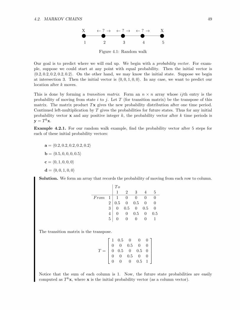
y y y y yX X← ? → ← ? → ← ? →
1 2 3 4 5
Figure 4.1: Random walk
Our goal is to predict where we will end up. We begin with a probability vector. For exam-ple, suppose we could start at any point with equal probability. Then the initial vector is〈0.2, 0.2, 0.2, 0.2, 0.2〉. On the other hand, we may know the initial state. Suppose we beginat intersection 3. Then the initial vector is 〈0, 0, 1, 0, 0〉. In any case, we want to predict ourlocation after k moves.
This is done by forming a transition matrix. Form an n × n array whose ijth entry is theprobability of moving from state i to j. Let T (for transition matrix) be the transpose of thismatrix. The matrix product Tx gives the new probability distribution after one time period.Continued left-multiplication by T gives the probabilities for future states. Thus for any initialprobability vector x and any positive integer k, the probability vector after k time periods isy = T kx.
Example 4.2.1. For our random walk example, find the probability vector after 5 steps foreach of these initial probability vectors:
a = 〈0.2, 0.2, 0.2, 0.2, 0.2〉
b = 〈0.5, 0, 0, 0, 0.5〉
c = 〈0, 1, 0, 0, 0〉
d = 〈0, 0, 1, 0, 0〉
Solution. We form an array that records the probability of moving from each row to column.
To1 2 3 4 5
From 1 1 0 0 0 02 0.5 0 0.5 0 03 0 0.5 0 0.5 04 0 0 0.5 0 0.55 0 0 0 0 1
The transition matrix is the transpose.
T =
1 0.5 0 0 00 0 0.5 0 00 0.5 0 0.5 00 0 0.5 0 00 0 0 0.5 1
Notice that the sum of each column is 1. Now, the future state probabilities are easilycomputed as T kx, where x is the initial probability vector (as a column vector).
50 CHAPTER 4. EIGENVALUE PROBLEMS
>> T = [ 1 0 .5 0 0 0 ; 0 0 0 .5 0 0 ; 0 0 .5 0 0 .5 0 ; 0 0 0 .5 0 0 ; 0 0 00 .5 1 ] ;
>> a = [ 0 . 2 ; 0 . 2 ; 0 . 2 ; 0 . 2 ; 0 . 2 ] ;>> b = [ 0 . 5 ; 0 ; 0 ; 0 ; 0 . 5 ] ;>> c = [ 0 ; 1 ; 0 ; 0 ; 0 ] ;>> d = [ 0 ; 0 ; 1 ; 0 ; 0 ] ;>> Tˆ5*aans =
0.4500000.0250000.0500000.0250000.450000
>> Tˆ5*bans =
0.500000.000000.000000.000000.50000
>> Tˆ5* cans =
0.687500.000000.125000.000000.18750
>> Tˆ5*dans =
0.375000.125000.000000.125000.37500
We notice that b results in no change from the initial probability.
A probability vector x is an equilibrium vector if x = Tx where T is the transition matrix for theMarkov chain. An equilibrium vector is one which results in no change moving to future states.Every Markov chain has at least one equilibrium vector and the eigenvalues of the transitionmatrix are the key to finding it.
Theorem 4.2.2. Let T be the transition matrix for a Markov chain. Then λ = 1 is an eigenvalueof T . If x is an eigenvector for λ = 1 with nonnegative components that sum to 1, then x is anequilibrium vector for T .
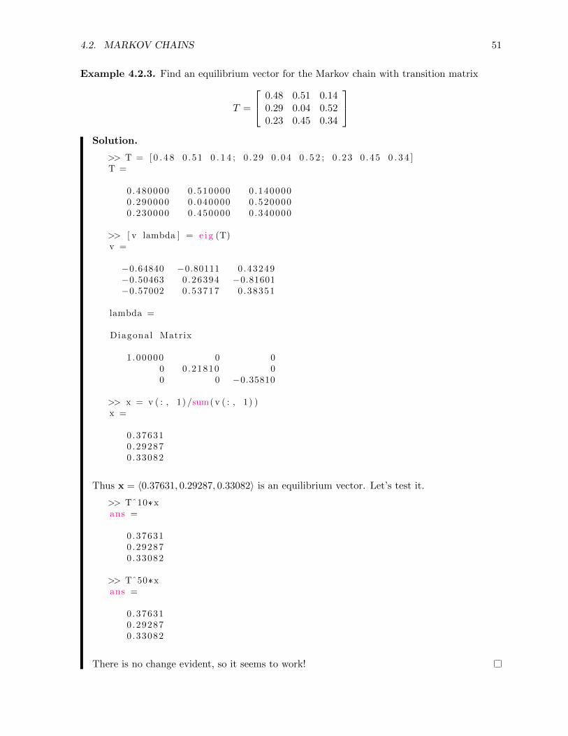
4.2. MARKOV CHAINS 51
Example 4.2.3. Find an equilibrium vector for the Markov chain with transition matrix
T =
0.48 0.51 0.140.29 0.04 0.520.23 0.45 0.34
Solution.
>> T = [ 0 . 4 8 0 .51 0 . 1 4 ; 0 .29 0 .04 0 . 5 2 ; 0 .23 0 .45 0 . 3 4 ]T =
0.480000 0.510000 0.1400000.290000 0.040000 0.5200000.230000 0.450000 0.340000
>> [ v lambda ] = e i g (T)v =
−0.64840 −0.80111 0.43249−0.50463 0.26394 −0.81601−0.57002 0.53717 0.38351
lambda =
Diagonal Matrix
1 .00000 0 00 0.21810 00 0 −0.35810
>> x = v ( : , 1) /sum( v ( : , 1) )x =
0.376310.292870.33082
Thus x = 〈0.37631, 0.29287, 0.33082〉 is an equilibrium vector. Let’s test it.
>> Tˆ10*xans =
0.376310.292870.33082
>> Tˆ50*xans =
0.376310.292870.33082
There is no change evident, so it seems to work!
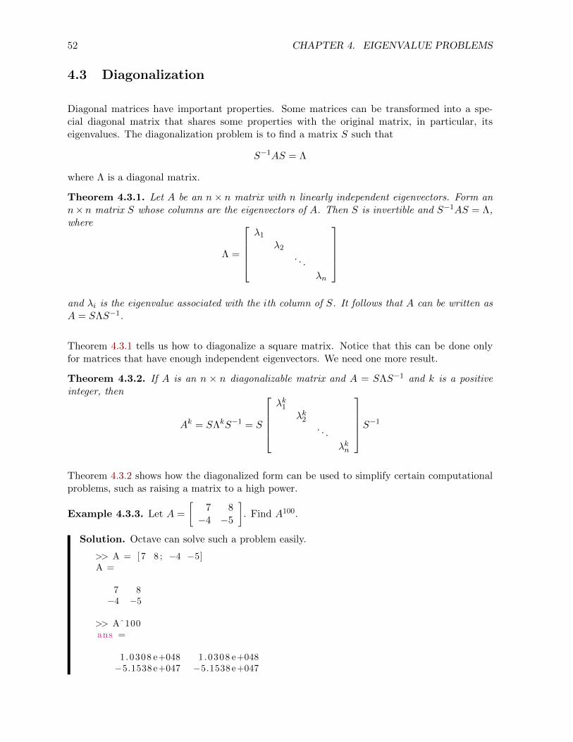
52 CHAPTER 4. EIGENVALUE PROBLEMS
4.3 Diagonalization
Diagonal matrices have important properties. Some matrices can be transformed into a spe-cial diagonal matrix that shares some properties with the original matrix, in particular, itseigenvalues. The diagonalization problem is to find a matrix S such that
S−1AS = Λ
where Λ is a diagonal matrix.
Theorem 4.3.1. Let A be an n× n matrix with n linearly independent eigenvectors. Form ann×n matrix S whose columns are the eigenvectors of A. Then S is invertible and S−1AS = Λ,where
Λ =
λ1
λ2. . .
λn
and λi is the eigenvalue associated with the ith column of S. It follows that A can be written asA = SΛS−1.
Theorem 4.3.1 tells us how to diagonalize a square matrix. Notice that this can be done onlyfor matrices that have enough independent eigenvectors. We need one more result.
Theorem 4.3.2. If A is an n × n diagonalizable matrix and A = SΛS−1 and k is a positiveinteger, then
Ak = SΛkS−1 = S
λk1
λk2. . .
λkn
S−1
Theorem 4.3.2 shows how the diagonalized form can be used to simplify certain computationalproblems, such as raising a matrix to a high power.
Example 4.3.3. Let A =
[7 8−4 −5
]. Find A100.
Solution. Octave can solve such a problem easily.
>> A = [ 7 8 ; −4 −5]A =
7 8−4 −5
>> Aˆ100ans =
1.0308 e+048 1 .0308 e+048−5.1538 e+047 −5.1538 e+047
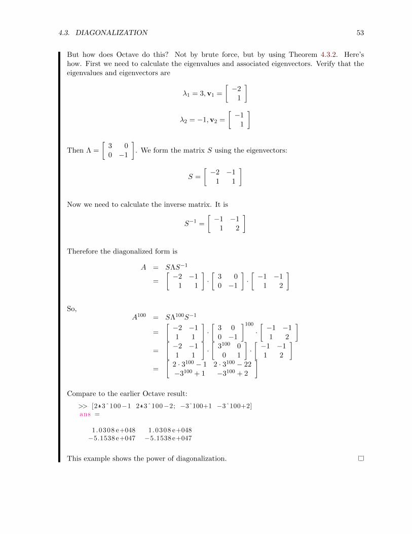
4.3. DIAGONALIZATION 53
But how does Octave do this? Not by brute force, but by using Theorem 4.3.2. Here’show. First we need to calculate the eigenvalues and associated eigenvectors. Verify that theeigenvalues and eigenvectors are
λ1 = 3,v1 =
[−2
1
]
λ2 = −1,v2 =
[−1
1
]
Then Λ =
[3 00 −1
]. We form the matrix S using the eigenvectors:
S =
[−2 −1
1 1
]
Now we need to calculate the inverse matrix. It is
S−1 =
[−1 −1
1 2
]
Therefore the diagonalized form is
A = SΛS−1
=
[−2 −1
1 1
]·[
3 00 −1
]·[−1 −1
1 2
]
So,A100 = SΛ100S−1
=
[−2 −11 1
]·[
3 00 −1
]100·[−1 −11 2
]=
[−2 −11 1
]·[
3100 00 1
]·[−1 −11 2
]=
[2 · 3100 − 1 2 · 3100 − 22−3100 + 1 −3100 + 2
]
Compare to the earlier Octave result:
>> [2*3ˆ100−1 2*3ˆ100−2; −3ˆ100+1 −3ˆ100+2]ans =
1.0308 e+048 1 .0308 e+048−5.1538 e+047 −5.1538 e+047
This example shows the power of diagonalization.
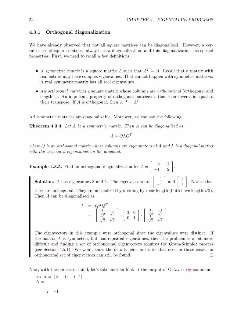
54 CHAPTER 4. EIGENVALUE PROBLEMS
4.3.1 Orthogonal diagonalization
We have already observed that not all square matrices can be diagonalized. However, a cer-tain class of square matrices always has a diagonalization, and this diagonalization has specialproperties. First, we need to recall a few definitions.
� A symmetric matrix is a square matrix A such that AT = A. Recall that a matrix withreal entries may have complex eigenvalues. That cannot happen with symmetric matrices.A real symmetric matrix has all real eigenvalues.
� An orthogonal matrix is a square matrix whose columns are orthonormal (orthogonal andlength 1). An important property of orthogonal matrices is that their inverse is equal totheir transpose: If A is orthogonal, then A−1 = AT .
All symmetric matrices are diagonalizable. Moreover, we can say the following:
Theorem 4.3.4. Let A be a symmetric matrix. Then A can be diagonalized as
A = QΛQT
where Q is an orthogonal matrix whose columns are eigenvectors of A and Λ is a diagonal matrixwith the associated eigenvalues on the diagonal.
Example 4.3.5. Find an orthogonal diagonalization for A =
[2 −1−1 2
].
Solution. A has eigenvalues 3 and 1. The eigenvectors are
[1−1
]and
[11
]. Notice that
these are orthogonal. They are normalized by dividing by their length (both have length√
2).Then A can be diagonalized as
A = QΛQT
=
[1√2
1√2
−1√2
1√2
]·[
3 00 1
]·
[1√2−1√2
1√2
1√2
]
The eigenvectors in this example were orthogonal since the eigenvalues were distinct. Ifthe matrix A is symmetric, but has repeated eigenvalues, then the problem is a bit moredifficult and finding a set of orthonormal eigenvectors requires the Gram-Schmidt process(see Section 4.5.1). We won’t show the details here, but note that even in those cases, anorthonormal set of eigenvectors can still be found.
Now, with these ideas in mind, let’s take another look at the output of Octave’s eig command.
>> A = [ 2 −1; −1 2 ]A =
2 −1
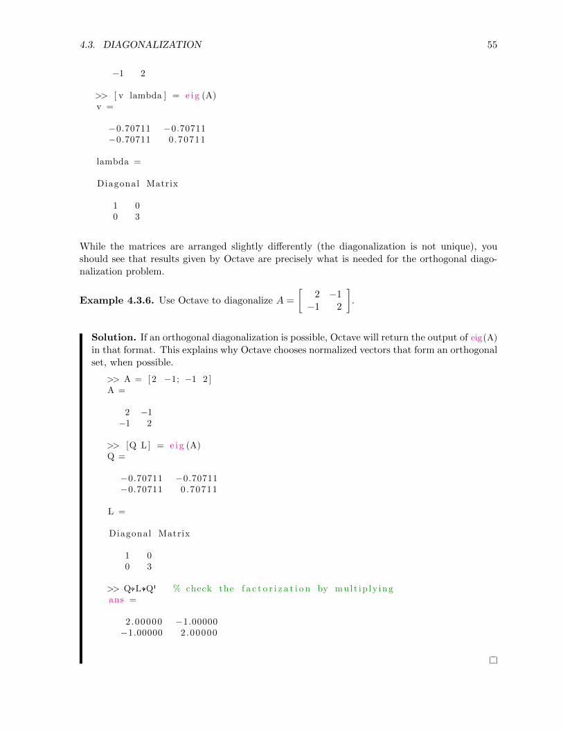
4.3. DIAGONALIZATION 55
−1 2
>> [ v lambda ] = e i g (A)v =
−0.70711 −0.70711−0.70711 0.70711
lambda =
Diagonal Matrix
1 00 3
While the matrices are arranged slightly differently (the diagonalization is not unique), youshould see that results given by Octave are precisely what is needed for the orthogonal diago-nalization problem.
Example 4.3.6. Use Octave to diagonalize A =
[2 −1−1 2
].
Solution. If an orthogonal diagonalization is possible, Octave will return the output of eig(A)
in that format. This explains why Octave chooses normalized vectors that form an orthogonalset, when possible.
>> A = [ 2 −1; −1 2 ]A =
2 −1−1 2
>> [Q L ] = e i g (A)Q =
−0.70711 −0.70711−0.70711 0.70711
L =
Diagonal Matrix
1 00 3
>> Q*L*Q' % check the f a c t o r i z a t i o n by mul t ip ly ingans =
2.00000 −1.00000−1.00000 2.00000
56 CHAPTER 4. EIGENVALUE PROBLEMS
4.4 Singular value decomposition
We are now prepared to tackle the singular value decomposition (SVD). This factorization issomething of a generalized version of what we just did for symmetric matrices in Section 4.3.1.But, the singular value decomposition exists for any matrix; the matrix need not even be square!The key is to consider the matrices ATA and AAT . These are always square symmetric matrices,and so, can be orthogonally diagonalized.
There are many applications associated with the SVD. Netflix recently sponsored a competitionwith a one million dollar prize to improve their movie recommendation algorithm. The teamthat won used a method based in part on the SVD2, which can be used to discover hiddenrelationships among variables. We will consider applications to least-squares problems andimage compression.
Theorem 4.4.1. Let A be an m × n matrix. The square roots of the nonzero eigenvalues ofATA and AAT (they are the same) are called the singular values of A,denoted σ1, σ2, . . . , σr.Then A can be factored as
A = UΣV T
where the columns of U are eigenvectors of AAT , the columns of V are eigenvectors of ATA,and the r singular values of A are on the diagonal of Σ. This factorization is called the singularvalue decomposition of A.
� U is m×m and orthogonal
� V is n× n and orthogonal
� Σ is m× n and diagonal of the special form
Σ =
σ1
...σ2 0
. . ....
σr· · · 0 · · · 0
If all the eigenvalues of ATA are distinct, then the associated eigenvectors are “automatically”orthogonal. We only need to make them unit vectors. If there are repeated eigenvalues, itis still possible to choose orthogonal eigenvectors, but more advanced methods are needed (seeSection 4.5.1). Our procedure starts with eigenvectors of ATA, then appropriate orthogonal uniteigenvectors for AAT are found using a simple formula, rather than by direct computation. Thenumber of singular values (nonzero eigenvalues) corresponds to the rank of the original matrixA. We will only consider examples where the number of singular values r is equal to m, thenumber of rows of A, otherwise, again, more advanced methods are required. We will consider
2http://buzzard.ups.edu/courses/2014spring/420projects/math420-UPS-spring-2014-gower-netflix-
SVD.pdf
4.4. SINGULAR VALUE DECOMPOSITION 57
a simple example using a 2× 2 matrix, then see how Octave commands can be used to find theSVD for larger or more difficult matrices.
Here is the simplified procedure we will use:
1. Find ATA.
2. Find the eigenvalues of ATA. The square roots of these are the singular values σ1, σ2, . . .,σr, arranged in decreasing order.
3. Find the corresponding eigenvectors and make them unit vectors v1,v2, . . . ,vn.
4. Find the vectors ui by computing ui =1
σiAvi.
5. Then A = UΣV T , where σ1, σ2, . . . , σr are on the diagonal of Σ and
U =[u1 u2 · · · um
]V =
[v1 v2 · · · vn
]� Remember to transpose V when you write the factorization.
� Remember to keep the eigenvalues and eigenvectors in their correct order.
� This simplified procedure only works if ATA has no repeated eigenvalues and r = m.
Example 4.4.2. Let A =
[4 4−3 3
]. Find the SVD via the simplified procedure outlined
above, then compare to the results obtained using the Octave function svd.
Solution. We can readily verify that rank(A) = 2, so the matrix should have two singularvalues.
>> A = [ 4 4 ; −3 3 ]A =
4 4−3 3
>> ATA = A' *AATA =
25 77 25
>> [ v lambda ] = e i g (ATA)v =
−0.70711 0.707110.70711 0.70711
lambda =
58 CHAPTER 4. EIGENVALUE PROBLEMS
Diagonal Matrix
18 00 32
Notice that the given eigenvectors are orthogonal unit vectors. However, the eigenvalues arenot in decreasing order. So, we need to switch the order of both eigenvectors and singularvalues (they must be in decreasing order) as we build V and Σ.
>> Sigma = ze ro s (2 , 2) ;>> Sigma (1 , 1) = s q r t ( lambda (2 , 2) )Sigma =
5.65685 0.000000.00000 0.00000
>> Sigma (2 , 2) = s q r t ( lambda (1 , 1) )Sigma =
5.65685 0.000000.00000 4.24264
>> V( : , 1) = v ( : , 2)V =
0.707110.70711
>> V( : , 2) = v ( : , 1)V =
0.70711 −0.707110.70711 0.70711
Now we build U to complete the factorization.
>> U( : , 1) = 1/Sigma (1 , 1) *A*V( : , 1)U =
1.000000.00000
>> U( : , 2) = 1/Sigma (2 , 2) *A*V( : , 2)U =
1.00000 0.000000.00000 1.00000
Now, let’s verify that UΣV T = A.
>> U*Sigma*V'
ans =
4.4. SINGULAR VALUE DECOMPOSITION 59
4 .0000 4 .0000−3.0000 3 .0000
Now that we have a rough sense of how an SVD is determined, let’s try the built-in Octavefunction. The command [U, S, V] = svd(A) computes the SVD of a matrix A and stores theresult in matrices U, S, and V. Let’s use this command to find the SVD of the matrix A andverify that U*S*V' returns A.
>> [U S V] = svd (A) % 3−output format o f svd commandU =
−1 00 1
S =
Diagonal Matrix
5 .6569 00 4 .2426
V =
−0.70711 −0.70711−0.70711 0.70711
>> U*S*V'
ans =
4.0000 4 .0000−3.0000 3 .0000
Notice that the factorization returned by svd is slightly different than we obtained above.This is normal: the SVD is not unique due to variations in how representative eigenvectorsare chosen.
4.4.1 Least squares
In Section 2.2, we used the normal equations, ATAx = ATb, to solve least-squares prob-lems. One potential problem with this approach is that the normal equations are typicallyill-conditioned. This means that a small change in the data can lead to a large change in the nu-meric solution. This is bad! One way to avoid this computational problem is to use a generalizedinverse known as the pseudoinverse, based on the SVD.
Theorem 4.4.3. For an m × n matrix A with singular value decomposition A = UΣV T , theleast-squares solution to the system Ax = b is given by
x = A+b
whereA+ = V Σ+UT
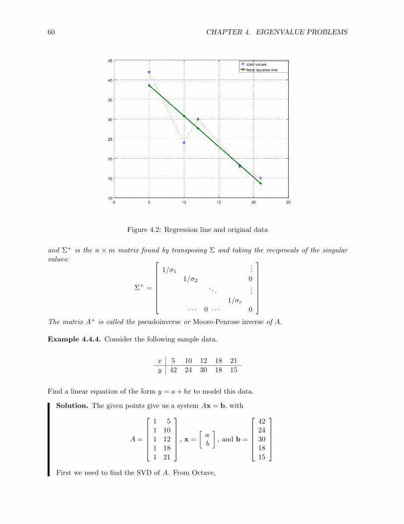
60 CHAPTER 4. EIGENVALUE PROBLEMS
Figure 4.2: Regression line and original data
and Σ+ is the n ×m matrix found by transposing Σ and taking the reciprocals of the singularvalues:
Σ+ =
1/σ1
...1/σ2 0
. . ....
1/σr· · · 0 · · · 0
The matrix A+ is called the pseudoinverse or Moore-Penrose inverse of A.
Example 4.4.4. Consider the following sample data.
x 5 10 12 18 21
y 42 24 30 18 15
Find a linear equation of the form y = a+ bx to model this data.
Solution. The given points give us a system Ax = b, with
A =
1 51 101 121 181 21
, x =
[ab
], and b =
4224301815
First we need to find the SVD of A. From Octave,
4.4. SINGULAR VALUE DECOMPOSITION 61
>> [U S V] = svd (A)U =
0.156839 0.767088 −0.427793 −0.340442 −0.2967660.311700 0.407114 −0.027649 0.469589 0.7182080.373645 0.263125 0.857417 −0.162313 −0.1721780.559478 −0.168843 −0.189306 0.580804 −0.5341410.652394 −0.384827 −0.212668 −0.547638 0.284878
S =
Diagonal Matrix
32.22136 00 0.885460 00 00 0
V =
0.063748 0.9979660.997966 −0.063748
Next, we construct Σ+ by taking the transpose of Σ (called S in our Octave code) and thereciprocal of the nonzero entries:
Σ+ =
[1/32.22136 0 0 0 0
0 1/0.88546 0 0 0
]=
[0.031035 0.000000 0.000000 0.000000 0.0000000.000000 0.885459 0.000000 0.000000 0.000000
]
After saving Σ+ as SP, the pseudoinverse, A+, can be calculated as:
>> Aplus = V*SP*U'
Aplus =
0.864865 0.459460 0.297297 −0.189189 −0.432432−0.050369 −0.019656 −0.007371 0.029484 0.047912
Thus the pseudoinverse is:
A+ ≈[
0.864865 0.459460 0.297297 −0.189189 −0.432432−0.050369 −0.019656 −0.007371 0.029484 0.047912
]
Finally, we are prepared to solve the original system of equations. The least-squares solution
is simply A+b, easily computed in Octave. The (approximate) solution vector is
[46.3784−1.5590
].
So, the correct linear equation is y = 46.3784 − 1.5590x. The original data and best-fittingline are shown in Figure 4.2.
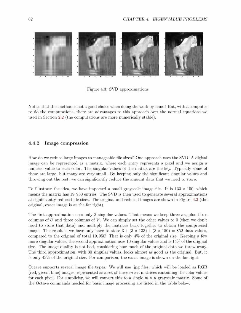
62 CHAPTER 4. EIGENVALUE PROBLEMS
Figure 4.3: SVD approximations
Notice that this method is not a good choice when doing the work by-hand! But, with a computerto do the computations, there are advantages to this approach over the normal equations weused in Section 2.2 (the computations are more numerically stable).
4.4.2 Image compression
How do we reduce large images to manageable file sizes? One approach uses the SVD. A digitalimage can be represented as a matrix, where each entry represents a pixel and we assign anumeric value to each color. The singular values of the matrix are the key. Typically some ofthese are large, but many are very small. By keeping only the significant singular values andthrowing out the rest, we can significantly reduce the amount data that we need to store.
To illustrate the idea, we have imported a small grayscale image file. It is 133 × 150, whichmeans the matrix has 19, 950 entries. The SVD is then used to generate several approximationsat significantly reduced file sizes. The original and reduced images are shown in Figure 4.3 (theoriginal, exact image is at the far right).
The first approximation uses only 3 singular values. That means we keep three σs, plus threecolumns of U and three columns of V . We can simply set the other values to 0 (then we don’tneed to store that data) and multiply the matrices back together to obtain the compressedimage. The result is we have only have to store 3 + (3 × 133) + (3 × 150) = 852 data values,compared to the original of total 19, 950! That is only 4% of the original size. Keeping a fewmore singular values, the second approximation uses 10 singular values and is 14% of the originalsize. The image quality is not bad, considering how much of the original data we threw away.The third approximation, with 30 singular values, looks almost as good as the original. But, itis only 43% of the original size. For comparison, the exact image is shown on the far right.
Octave supports several image file types. We will use .jpg files, which will be loaded as RGB(red, green, blue) images, represented as a set of three m×n matrices containing the color valuesfor each pixel. For simplicity, we will convert this to a single m× n grayscale matrix. Some ofthe Octave commands needed for basic image processing are listed in the table below.
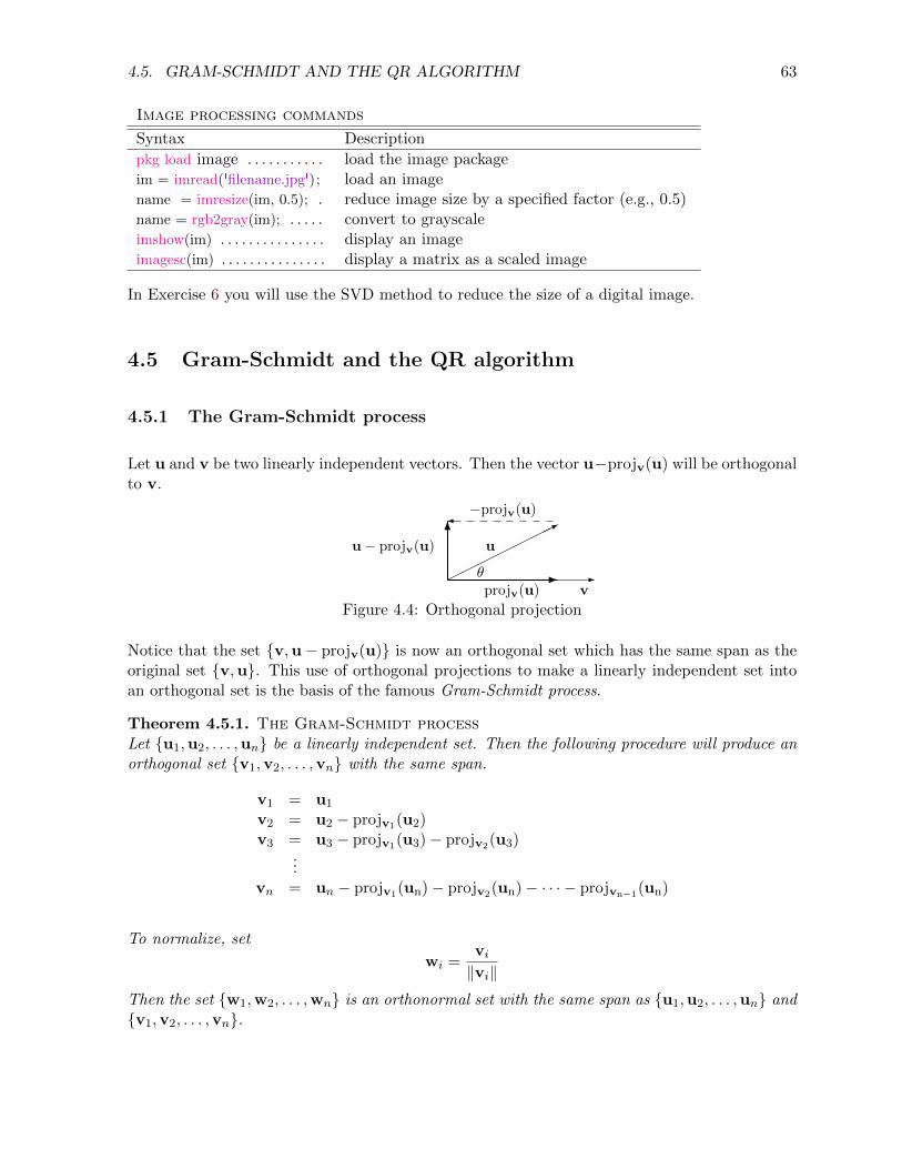
4.5. GRAM-SCHMIDT AND THE QR ALGORITHM 63
Image processing commands
Syntax Description
pkg load image . . . . . . . . . . . load the image packageim = imread('filename.jpg'); load an imagename = imresize(im, 0.5); . reduce image size by a specified factor (e.g., 0.5)name = rgb2gray(im); . . . . . convert to grayscaleimshow(im) . . . . . . . . . . . . . . . display an imageimagesc(im) . . . . . . . . . . . . . . . display a matrix as a scaled image
In Exercise 6 you will use the SVD method to reduce the size of a digital image.
4.5 Gram-Schmidt and the QR algorithm
4.5.1 The Gram-Schmidt process
Let u and v be two linearly independent vectors. Then the vector u−projv(u) will be orthogonalto v.
-���
���
��*�
-
6
θ
u
projv(u) v
u− projv(u)
−projv(u)
Figure 4.4: Orthogonal projection
Notice that the set {v,u− projv(u)} is now an orthogonal set which has the same span as theoriginal set {v,u}. This use of orthogonal projections to make a linearly independent set intoan orthogonal set is the basis of the famous Gram-Schmidt process.
Theorem 4.5.1. The Gram-Schmidt processLet {u1,u2, . . . ,un} be a linearly independent set. Then the following procedure will produce anorthogonal set {v1,v2, . . . ,vn} with the same span.
v1 = u1
v2 = u2 − projv1(u2)v3 = u3 − projv1(u3)− projv2(u3)
...vn = un − projv1(un)− projv2(un)− · · · − projvn−1(un)
To normalize, set
wi =vi‖vi‖
Then the set {w1,w2, . . . ,wn} is an orthonormal set with the same span as {u1,u2, . . . ,un} and{v1,v2, . . . ,vn}.
64 CHAPTER 4. EIGENVALUE PROBLEMS
Example 4.5.2. Find an orthonormal set with the same span as
{〈10, 9,−3, 0〉, 〈−7, 7,−3, 4〉, 〈9, 1,−8,−1〉}
Solution. Since we are going to make extensive use of vector projections, it would be a goodidea to write a function that handles that part of the computation. This can be entered atthe command line, or better yet, it can be saved in a function file ‘proj.m’ and reused infuture problems.
>> f unc t i on vect = pro j (u , v )vect = dot (u , v ) / dot (v , v ) *v ;
end
As defined, proj(u, v) now computes the projection of u onto v.
Now, we will enter the original set of vectors as columns in a matrix U .
>> U = [10 −7 9 ; 9 7 1 ; −3 −3 −8; 0 4 −1]U =
10 −7 99 7 1−3 −3 −8
0 4 −1
Next, we go through the steps of the Gram-Schmidt process to create a matrix V whosecolumns are an orthogonal set with the same span as the original set.
>> V = ze ro s (4 , 3) ;>> V( : , 1) = U( : , 1) ;>> V( : , 2) = U( : , 2) − pro j (U( : , 2) , V( : , 1) ) ;>> V( : , 3) = U( : , 3) − pro j (U( : , 3) , V( : , 1) ) − pro j (U( : , 3) , V( : , 2) )V =
10.00000 −7.10526 0.371579.00000 6.90526 −2.73222−3.00000 −2.96842 −6.95810
0.00000 4.00000 0.21304
These vectors are orthogonal, but not yet unit vectors, so we normalize. The final outputmatrix W should have columns that are orthogonal unit vectors with the same span as theoriginal set.
>> W = zero s (4 , 3) ;>> W( : , 1) = V( : , 1) /norm(V( : , 1) ) ;>> W( : , 2) = V( : , 2) /norm(V( : , 2) ) ;>> W( : , 3) = V( : , 3) /norm(V( : , 3) )W =
0.72548 −0.64071 0.049620.65293 0.62268 −0.36490−0.21764 −0.26768 −0.92929
0.00000 0.36070 0.02845
The columns of W are the desired orthonormal set.
4.5. GRAM-SCHMIDT AND THE QR ALGORITHM 65
We might want to verify that the process worked. As a spot check, we can look at the dotproduct of any two columns and we should get 0. Also, each column should have norm 1.
>> dot (W( : , 1) , W( : , 3) )ans = 2.2204 e−016>> norm(W( : , 3) )ans = 1
Notice that the dot product is not quite zero due to rounding error, but the results are more thanadequate for our purposes. We should note that the Gram-Schmidt algorithm in its classic formis known to be numerically unstable. Consult a numerical linear algebra book for details aboutsome simple modifications that can reduce the loss of orthogonality due to round-off error3.
4.5.2 QR decomposition
We have already seen several important matrix factorizations. The Gram-Schmidt process is thekey to another, one that turns out to provide a good means for finding eigenvalues numerically.This is known as the QR decomposition.
Theorem 4.5.3. Let A be a nonsingular square matrix. Then there exists an orthogonal matrixQ and an upper triangular matrix R such that A = QR.
Here’s how to find Q and R.
1. Apply the Gram-Schmidt process to the columns of A. Use the resulting orthonormalvectors as columns of Q.
2. Let R =
q1 · a1 q1 · a2 q1 · a3 · · · q1 · an
0 q2 · a2 q2 · a3 · · · q2 · an0 0 q3 · a3 · · · q3 · an...
......
. . ....
0 0 0 0 qn · an
, where qi is the ith column of Q and
aj is the jth column of A.
Example 4.5.4. Find the QR decomposition of the matrix A =
5 7 010 8 05 6 −5
.
Solution. First we apply the Gram-Schmidt process to A.
>> A = [ 5 7 0 ; 10 8 0 ; 5 6 −5]A =
5 7 010 8 0
5 6 −5
3Or try an internet search for ‘numerical instability Gram-Schmidt’ and you will find many explanations andmodified code examples.
66 CHAPTER 4. EIGENVALUE PROBLEMS
>> Q = ze ro s (3 , 3) ;>> Q( : , 1) = A( : , 1) /norm(A( : , 1) ) ;>> Q( : , 2) = A( : , 2) − pro j (A( : , 2) ,Q( : , 1) ) ;>> Q( : , 2) = Q( : , 2) /norm(Q( : , 2) ) ;>> Q( : , 3) = A( : , 3) − pro j (A( : , 3) , Q( : , 1) ) − pro j (A( : , 3) , Q( : , 2) )
;>> Q( : , 3) = Q( : , 3) /norm(Q( : , 3) )Q =
0.40825 0.72900 0.549440.81650 −0.56077 0.137360.40825 0.39254 −0.82416
Notice that we normalized each vector as we went through the process to find Q. Now, let’sverify that Q is orthogonal. For an orthogonal matrix, Q−1 = QT , so a good way to checkfor orthogonality is to compute QTQ, which should be an identity matrix.
>> Q' *Qans =
1.00000 −0.00000 0.00000−0.00000 1.00000 −0.00000
0.00000 −0.00000 1.00000
This looks correct (some round-off error can be seen if we check more digits than displayedhere). Now, we build R using the appropriate dot products of columns of Q and A.
>> R = ze ro s (3 , 3) ;>> R(1 , 1) = dot (Q( : , 1) , A( : , 1) ) ;>> R(1 , 2) = dot (Q( : , 1) , A( : , 2) ) ;>> R(1 , 3) = dot (Q( : , 1) , A( : , 3) ) ;>> R(2 , 2) = dot (Q( : , 2) , A( : , 2) ) ;>> R(2 , 3) = dot (Q( : , 2) , A( : , 3) ) ;>> R(3 , 3) = dot (Q( : , 3) , A( : , 3) )R =
12.24745 11.83920 −2.041240.00000 2.97209 −1.962700.00000 0.00000 4.12082
Of course, for a larger problem, we would use loops to compute the entries in R. Finally wecheck to see that QR = A.
>> Q*Rans =
5.00000 7.00000 0.0000010.00000 8.00000 0.00000
5.00000 6.00000 −5.00000
It works as expected.
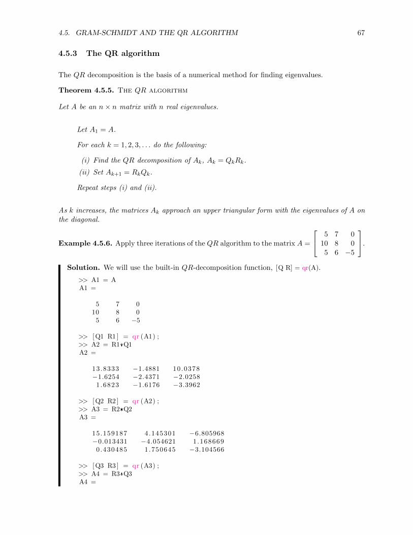
4.5. GRAM-SCHMIDT AND THE QR ALGORITHM 67
4.5.3 The QR algorithm
The QR decomposition is the basis of a numerical method for finding eigenvalues.
Theorem 4.5.5. The QR algorithm
Let A be an n× n matrix with n real eigenvalues.
Let A1 = A.
For each k = 1, 2, 3, . . . do the following:
(i) Find the QR decomposition of Ak, Ak = QkRk.
(ii) Set Ak+1 = RkQk.
Repeat steps (i) and (ii).
As k increases, the matrices Ak approach an upper triangular form with the eigenvalues of A onthe diagonal.
Example 4.5.6. Apply three iterations of the QR algorithm to the matrix A =
5 7 010 8 05 6 −5
.
Solution. We will use the built-in QR-decomposition function, [Q R] = qr(A).
>> A1 = AA1 =
5 7 010 8 0
5 6 −5
>> [Q1 R1 ] = qr (A1) ;>> A2 = R1*Q1A2 =
13.8333 −1.4881 10.0378−1.6254 −2.4371 −2.0258
1 .6823 −1.6176 −3.3962
>> [Q2 R2 ] = qr (A2) ;>> A3 = R2*Q2A3 =
15.159187 4.145301 −6.805968−0.013431 −4.054621 1.168669
0.430485 1.750645 −3.104566
>> [Q3 R3 ] = qr (A3) ;>> A4 = R3*Q3A4 =
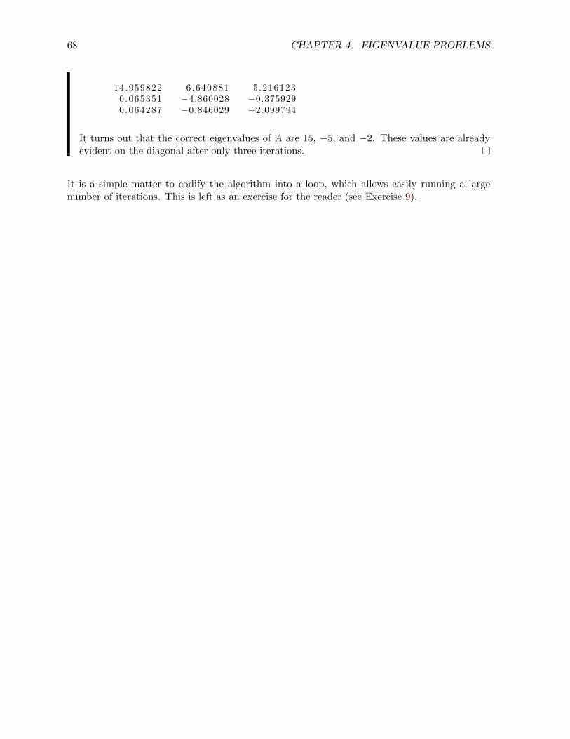
68 CHAPTER 4. EIGENVALUE PROBLEMS
14.959822 6.640881 5.2161230.065351 −4.860028 −0.3759290.064287 −0.846029 −2.099794
It turns out that the correct eigenvalues of A are 15, −5, and −2. These values are alreadyevident on the diagonal after only three iterations.
It is a simple matter to codify the algorithm into a loop, which allows easily running a largenumber of iterations. This is left as an exercise for the reader (see Exercise 9).
EXERCISES 69
Chapter 4 Exercises
1. Suppose a hypothetical state is divided into four regions, A, B, C, and D. Each year, acertain number of people will move from one region to another, changing the populationdistribution. The initial populations are given below:
Region Population
A 719B 910C 772D 807
The following table records how the population moved in one year.
ToA B C D
From A 624 79 2 14B 79 670 70 91C 52 6 623 91D 77 20 58 652
For example, we see that A began with 624 + 79 + 2 + 14 = 719 residents. Of these, 624stayed in A, 79 moved to B, 2 moved to C, and 14 moved to D. From this empirical data,we can give approximate probabilities for moving from A. Of the 719 residents, 624 stayedin A, so the probability of ‘moving’ from A to A is 624/719 = 0.8678720. The probabilityof moving from A to B is 79/719 = 0.1098748, and so on.
(a) Find the transition matrix T for this Markov chain. This is done by converting eachentry in the table above to a probability, then transposing.
(b) Express the initial population distribution as a probability vector x. Remember, thecomponents must add to 1.
(c) Find the population distribution (expressed as percentages) in 5 years and in 10 years.
(d) Compute the eigenvalues and eigenvectors for T and use the eigenvector for λ = 1 toconstruct an equilibrium vector q for this Markov chain. This represents a populationdistribution for which there is no further change from year to year. Verify that thedistribution is in equilibrium by computing several future states, such as T 25q andT 50q. Is there any change in the distribution?
2. Diagonalize the matrix A =
[1 41 −2
]as A = SΛS−1 and use this to calculate A50. Show
all the steps needed to find the eigenvalues, eigenvectors, etc.
3. Orthogonally diagonalize the symmetric matrix A =
1 1 31 1 33 3 9
. Verify that A = QΛQT
and show by direct calculation that Q is an orthogonal matrix.
4. Find the SVD of the matrix
[2 30 2
]without using the svd command. Show all the steps
needed to find the eigenvalues, eigenvectors, etc. Verify that A = UΣV T .
70 CHAPTER 4. EIGENVALUE PROBLEMS
5. Use the pseudoinverse to find the least-squares line y = a + bx through the given set ofpoints.
{(−1, 5), (1, 4), (2, 2.5), (3, 0)}
You may use the svd command, but show all the rest of the details, including constructionof the pseudoinverse. Include a plot of the data values and the least-squares line.
6. For this problem, you will use the SVD to produce a compressed image using n singularvalues. You choose n (something between 5 and 50 would be suitable). To begin, you willneed a digital photo in .JPG format.
(a) Load the image in Octave as ‘imcolor,’ then convert to a grayscale image. Check thesize of your grayscale image and if it is larger than approximately 320×280, determinean appropriate reduction factor and reduce it. Name the reduced, grayscale formatimage ‘im.’ This is the image that will be compressed via the SVD method. Displaythe reduced grayscale image using imagesc and verify that it still looks like the original.Include a copy of this grayscale image with your problem solutions and state its size.
Here is a summary of the commands needed for the initial image processing:
>> imco lor = imread ( ' photo . jpg ' ) ; % load image>> imgray = rgb2gray ( imco lor ) ; % make g r a y s c a l e>> s i z e ( imgray ) % check image s i z e>> im = i m r e s i z e ( imgray , f a c t o r ) % r e s i z e image>> imagesc ( im) % dip lay image matrix
(b) Find the SVD of the matrix representation ‘im.’ Calculate an approximation usingn singular values. That means you should only keep the first n columns of U , then largest values of Σ, and the first n columns of V . Set the other values to 0, thencompute UΣV T to recover an approximation of the original image. Save it as ‘im2’and display it using imagesc.
How many nonzero values are saved in the compressed factorization compared to theoriginal? Include a copy of the reduced image with your problem solution.
7. Write an Octave script that takes a matrix U with linearly independent columns andoutputs a matrix V with orthonormal columns. The core loop could look like this (or useyour own formulation):
V( : , 1) = U( : , 1) /norm(U( : , 1) ) ;f o r i = 2 : n
V( : , i ) = U( : , i ) ;f o r j = 1 : i−1
V( : , i ) = V( : , i ) − pro j (U( : , i ) , V( : , j ) ) ;endV( : , i ) = V( : , i ) /norm(V( : , i ) ) ;
end
You will need to determine m and n and from the dimensions of U and the functionproj(u,v) must be defined. Test your code on the vectors from Example 4.5.2.
8. Use your code from Exercise 7 as the starting point of a script file that computes the QRdecomposition of an n × n matrix A. Test your script on a randomly generated 4 × 4matrix, A = rand(4,4). Check Q for orthogonality by computing QTQ, which should be anidentity matrix, and verify that A = QR.
EXERCISES 71
9. Using Octave’s built-in [Q R] = qr(A) function for the QR decomposition, write a loop (atthe command line or in a script file) that will approximate the eigenvalues of the matrix
A =
1 −1 2−1 1 −2
2 −2 0
. Run your loop through ten iterations. The actual eigenvalues are
integers. Were you able to determine the correct values from the QR algorithm?

72 CHAPTER 4. EIGENVALUE PROBLEMS
Chapter 5
Additional topics
5.1 Three dimensional graphs
5.1.1 Space curves
Plotting a curve in 3-dimensions is similar to the 2-dimensional plotting explained in Section 1.3.To plot space curves, we use the command plot3(x, y, z), where x, y, and z correspond to theparametric equations for the function. For example, let’s plot a simple helix, with vector equationr(t) = sin(t)i+cos(t)j+tk. First we generate a row vector for the parameter t, then we calculatethe range for x, y, and z.
>> t = l i n s p a c e (0 , 2*pi , 30) ;>> x = s i n ( t ) ;>> y = cos ( t ) ;>> z = t ;>> p lo t3 (x , y , z )
The graph is shown in Figure 5.1.
Now consider a more complicated curve, like
x = (4 + sin 20t) cos t, y = (4 + sin 20t) sin t, z = cos 20t
This is a ‘toroidal spiral.’ We will need to use a much finer increment for t to get a smoothpicture.
>> t = l i n s p a c e (0 , 2*pi , 500) ;>> x = (5 + s i n (25* t ) ) .* cos ( t ) ;>> y = (5 + s i n (25* t ) ) .* s i n ( t ) ;>> z = cos (25* t ) ;>> p lo t3 (x , y , z )
These types of graphs are not easy to draw without a computer! See Figure 5.2.
73
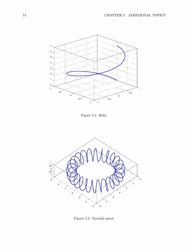
74 CHAPTER 5. ADDITIONAL TOPICS
Figure 5.1: Helix
Figure 5.2: Toroidal spiral
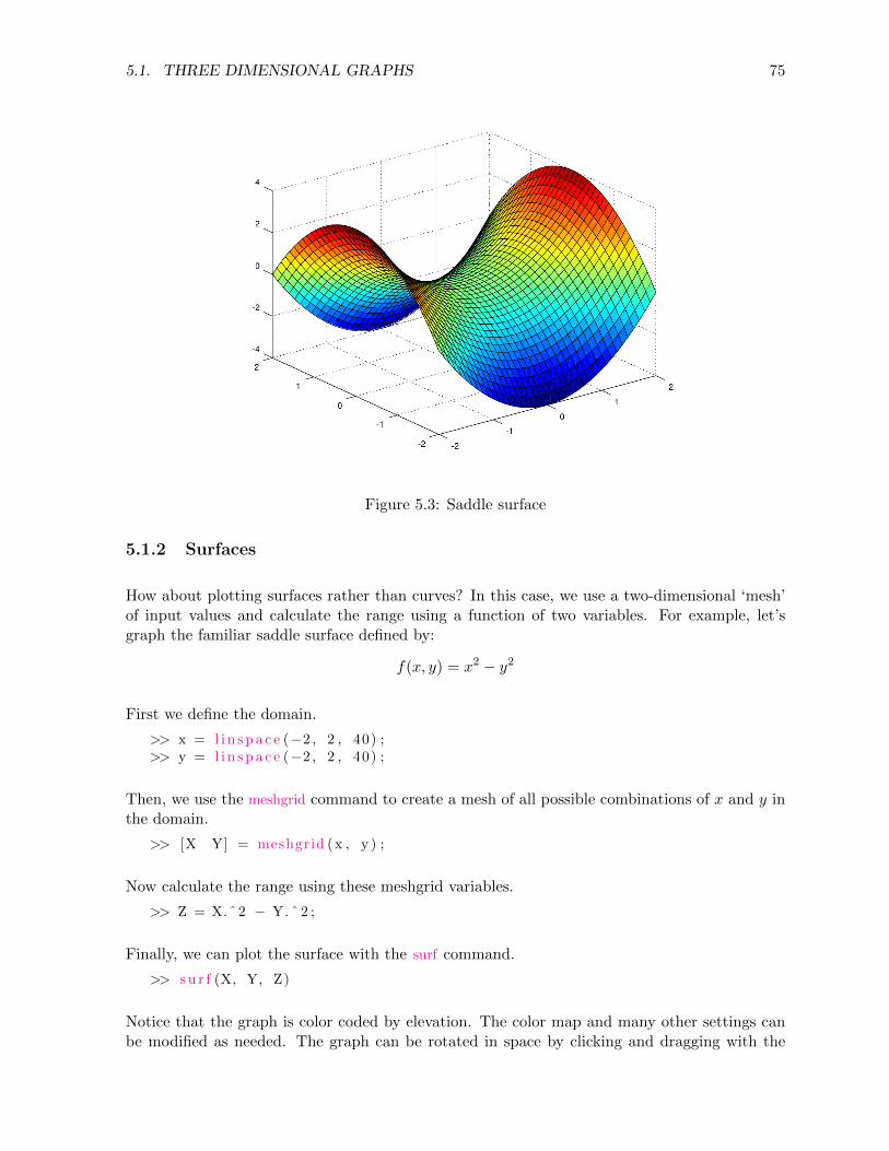
5.1. THREE DIMENSIONAL GRAPHS 75
Figure 5.3: Saddle surface
5.1.2 Surfaces
How about plotting surfaces rather than curves? In this case, we use a two-dimensional ‘mesh’of input values and calculate the range using a function of two variables. For example, let’sgraph the familiar saddle surface defined by:
f(x, y) = x2 − y2
First we define the domain.
>> x = l i n s p a c e (−2 , 2 , 40) ;>> y = l i n s p a c e (−2 , 2 , 40) ;
Then, we use the meshgrid command to create a mesh of all possible combinations of x and y inthe domain.
>> [X Y] = meshgrid (x , y ) ;
Now calculate the range using these meshgrid variables.
>> Z = X.ˆ2 − Y. ˆ 2 ;
Finally, we can plot the surface with the surf command.
>> s u r f (X, Y, Z)
Notice that the graph is color coded by elevation. The color map and many other settings canbe modified as needed. The graph can be rotated in space by clicking and dragging with the
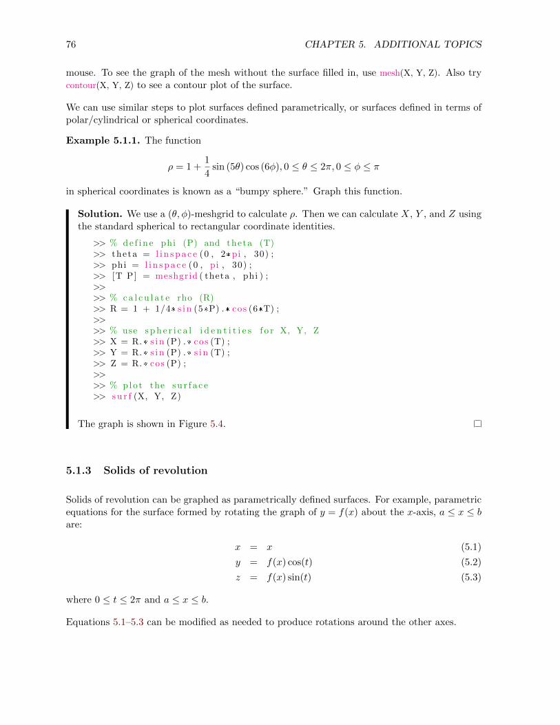
76 CHAPTER 5. ADDITIONAL TOPICS
mouse. To see the graph of the mesh without the surface filled in, use mesh(X, Y, Z). Also trycontour(X, Y, Z) to see a contour plot of the surface.
We can use similar steps to plot surfaces defined parametrically, or surfaces defined in terms ofpolar/cylindrical or spherical coordinates.
Example 5.1.1. The function
ρ = 1 +1
4sin (5θ) cos (6φ), 0 ≤ θ ≤ 2π, 0 ≤ φ ≤ π
in spherical coordinates is known as a “bumpy sphere.” Graph this function.
Solution. We use a (θ, φ)-meshgrid to calculate ρ. Then we can calculate X, Y , and Z usingthe standard spherical to rectangular coordinate identities.
>> % d e f i n e phi (P) and theta (T)>> theta = l i n s p a c e (0 , 2*pi , 30) ;>> phi = l i n s p a c e (0 , pi , 30) ;>> [T P] = meshgrid ( theta , phi ) ;>>>> % c a l c u l a t e rho (R)>> R = 1 + 1/4* s i n (5*P) .* cos (6*T) ;>>>> % use s p h e r i c a l i d e n t i t i e s f o r X, Y, Z>> X = R.* s i n (P) .* cos (T) ;>> Y = R.* s i n (P) .* s i n (T) ;>> Z = R.* cos (P) ;>>>> % plo t the s u r f a c e>> s u r f (X, Y, Z)
The graph is shown in Figure 5.4.
5.1.3 Solids of revolution
Solids of revolution can be graphed as parametrically defined surfaces. For example, parametricequations for the surface formed by rotating the graph of y = f(x) about the x-axis, a ≤ x ≤ bare:
x = x (5.1)
y = f(x) cos(t) (5.2)
z = f(x) sin(t) (5.3)
where 0 ≤ t ≤ 2π and a ≤ x ≤ b.
Equations 5.1–5.3 can be modified as needed to produce rotations around the other axes.
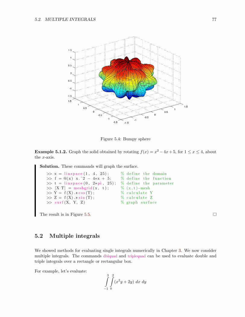
5.2. MULTIPLE INTEGRALS 77
Figure 5.4: Bumpy sphere
Example 5.1.2. Graph the solid obtained by rotating f(x) = x2− 4x+ 5, for 1 ≤ x ≤ 4, aboutthe x-axis.
Solution. These commands will graph the surface.
>> x = l i n s p a c e (1 , 4 , 25) ; % d e f i n e the domain>> f = @( x ) x .ˆ2 − 4*x + 5 ; % d e f i n e the func t i on>> t = l i n s p a c e (0 , 2*pi , 25) ; % d e f i n e the parameter>> [X T] = meshgrid (x , t ) ; % (x , t )−mesh>> Y = f (X) .* cos (T) ; % c a l c u l a t e Y>> Z = f (X) .* s i n (T) ; % c a l c u l a t e Z>> s u r f (X, Y, Z) % graph s u r f a c e
The result is in Figure 5.5.
5.2 Multiple integrals
We showed methods for evaluating single integrals numerically in Chapter 3. We now considermultiple integrals. The commands dblquad and triplequad can be used to evaluate double andtriple integrals over a rectangle or rectangular box.
For example, let’s evaluate:3∫−1
2∫0
(x2y + 2y) dx dy
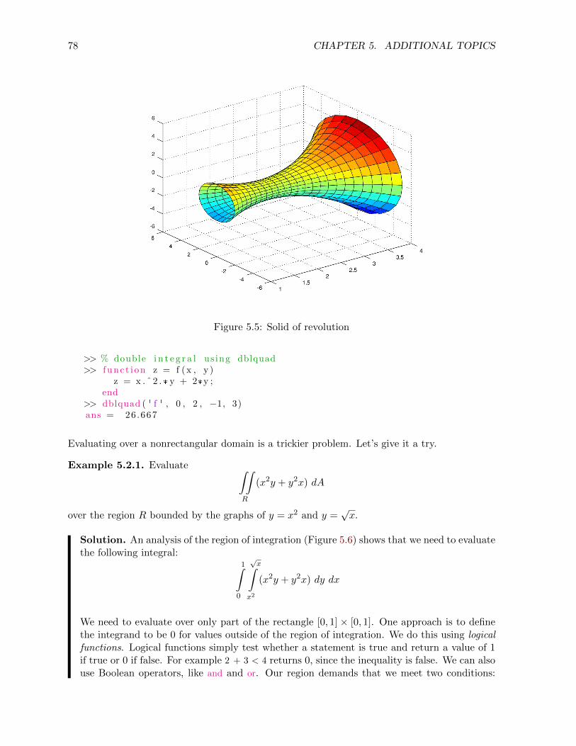
78 CHAPTER 5. ADDITIONAL TOPICS
Figure 5.5: Solid of revolution
>> % double i n t e g r a l us ing dblquad>> f unc t i on z = f (x , y )
z = x . ˆ 2 . * y + 2*y ;end
>> dblquad ( ' f ' , 0 , 2 , −1, 3)ans = 26.667
Evaluating over a nonrectangular domain is a trickier problem. Let’s give it a try.
Example 5.2.1. Evaluate ∫∫R
(x2y + y2x) dA
over the region R bounded by the graphs of y = x2 and y =√x.
Solution. An analysis of the region of integration (Figure 5.6) shows that we need to evaluatethe following integral:
1∫0
√x∫
x2
(x2y + y2x) dy dx
We need to evaluate over only part of the rectangle [0, 1] × [0, 1]. One approach is to definethe integrand to be 0 for values outside of the region of integration. We do this using logicalfunctions. Logical functions simply test whether a statement is true and return a value of 1if true or 0 if false. For example 2 + 3 < 4 returns 0, since the inequality is false. We can alsouse Boolean operators, like and and or. Our region demands that we meet two conditions:
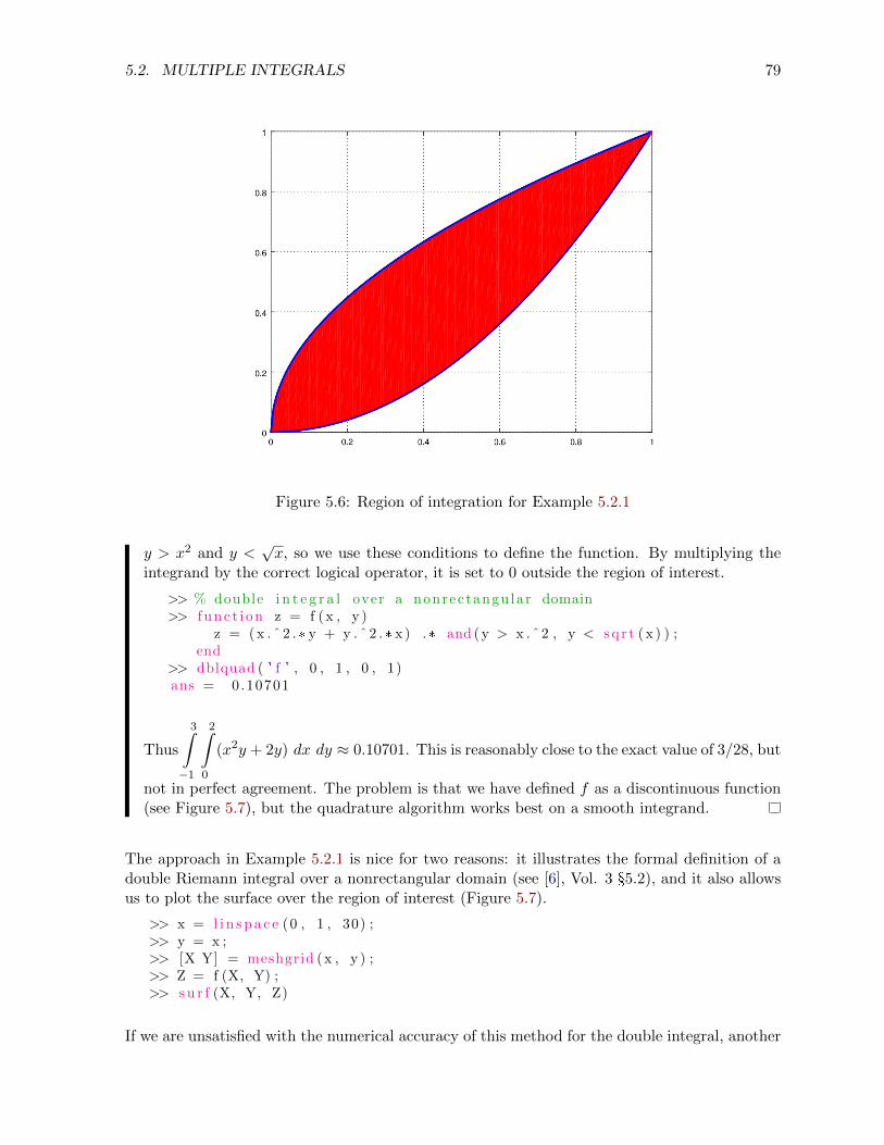
5.2. MULTIPLE INTEGRALS 79
Figure 5.6: Region of integration for Example 5.2.1
y > x2 and y <√x, so we use these conditions to define the function. By multiplying the
integrand by the correct logical operator, it is set to 0 outside the region of interest.
>> % double i n t e g r a l over a nonrectangu lar domain>> f unc t i on z = f (x , y )
z = ( x . ˆ 2 . * y + y . ˆ 2 . * x ) .* and ( y > x . ˆ 2 , y < s q r t ( x ) ) ;end
>> dblquad ( ' f ' , 0 , 1 , 0 , 1)ans = 0.10701
Thus
3∫−1
2∫0
(x2y + 2y) dx dy ≈ 0.10701. This is reasonably close to the exact value of 3/28, but
not in perfect agreement. The problem is that we have defined f as a discontinuous function(see Figure 5.7), but the quadrature algorithm works best on a smooth integrand.
The approach in Example 5.2.1 is nice for two reasons: it illustrates the formal definition of adouble Riemann integral over a nonrectangular domain (see [6], Vol. 3 §5.2), and it also allowsus to plot the surface over the region of interest (Figure 5.7).
>> x = l i n s p a c e (0 , 1 , 30) ;>> y = x ;>> [X Y] = meshgrid (x , y ) ;>> Z = f (X, Y) ;>> s u r f (X, Y, Z)
If we are unsatisfied with the numerical accuracy of this method for the double integral, another

80 CHAPTER 5. ADDITIONAL TOPICS
Figure 5.7: Solid volume for Example 5.2.1
approach is to use a change of variables to transform to a rectangular region of integration asfollows:
y = y1 + u(y2 − y1) (5.4)
dy = (y2 − y1) du (5.5)
Then as y ranges from y1 to y2, u ranges from 0 to 1 and the integrand becomes:
∫ x2
x1
∫ y2
y1
f(x, y) dy dx =
∫ x2
x1
∫ 1
0f(x, y1 + u(y2 − y1))(y2 − y1) du dx (5.6)
This is a bit cumbersome to enter in Octave. We’ll use a series of anonymous functions (seepage 35) to define the integrand, then try dblquad again.
Example 5.2.2. Use the change of variable formulas in Equations 5.4–5.6 to evaluate
1∫0
√x∫
x2
(x2y + y2x) dy dx
Solution.
>> f 1 = @(x , y ) x . ˆ 2 . * y + y . ˆ 2 . * x ;>> y1 = @( x ) x . ˆ 2 ;>> y2 = @( x ) s q r t ( x ) ;>> f 2 = @(x , u) f 1 (x , y1 ( x ) + u . * ( y2 ( x ) − y1 ( x ) ) ) .* ( y2 ( x ) − y1 ( x ) ) ;
5.2. MULTIPLE INTEGRALS 81
>> format long>> dblquad ( f2 , 0 , 1 , 0 , 1) % no quotes around anonymous func t i on nameans = 0.107142857143983>> 3/28 % compare r e s u l t to known exact answerans = 0.107142857142857
This approach gives a more satisfactory result.
If one wishes to evaluate many integrals of this form, writing a function file to automate theabove steps would be a good idea.
Example 5.2.3. Write an Octave function file that computes∫∫R
f(x, y) dA
over the region R bounded by the graphs of y = y1(x), y = y2(x), x = a, and x = b, using thechange of variables in Equations 5.4–5.6.
Solution. A function file is similar to script: it is a plain text .m-file containing a seriesof Octave commands. To be recognized as a function file, the first line of code (excludingcomments and white space) must be function. With the file placed in the load path, it can berun from the command line like any other Octave function. The function name should matchthe file name. A well written function file will include details like help text and provisions forerror checking. Refer to [3]. We will give a minimal example that accomplishes our changeof variables procedure.
Octave Script 5.1: Double integral function file
1 % func t i on f i l e ' d b l i n t .m'
2 % eva lua t e s dblquad ( f , x1 , x2 , y1 , y2 )3 % where f i s an anonymous func t i on o f x and y4 % y1 and y2 are anonymous f u n c t i o n s o f x5 % x1 and x2 are r e a l numbers6
7 f unc t i on va l = d b l i n t ( f , x1 , x2 , y1 , y2 )8 f 2 = @(x , u) f (x , y1 ( x ) + u . * ( y2 ( x ) − y1 ( x ) ) ) .* ( y2 ( x ) − y1 ( x ) ) ;9 dblquad ( f2 , x1 , x2 , 0 , 1)
10 end
Note that the comment lines at the top of our function file will be displayed if we typehelp dblint. Thus we should strive to put a good description of the syntax in those lines.Now, to use this function, saved in our working directory as ‘dblint.m,’ we need to define theintegrand, and the functions representing the limits of integration on y. Then we pass theseto our function dblint. Let’s try it on the integral from Example 5.2.1.
>> f = @(x , y ) x . ˆ 2 . * y + y . ˆ 2 . * x ;>> y1 = @( x ) x . ˆ 2 ;>> y2 = @( x ) s q r t ( x ) ;>> d b l i n t ( f , 0 , 1 , y1 , y2 )ans = 0.10714
It works!
82 CHAPTER 5. ADDITIONAL TOPICS
5.2.1 Double Riemann sums
Suppose we want to write our own algorithms for double integration. It is straightforwardto write an Octave script that will estimate a double integral over a rectangle using a doubleRiemann sum, taking sample points to be the upper right hand corners of the subrectangles in thepartition. For our example, we’ll use the function f(x, y) = x+2y2, defined on R = [0, 2]× [0, 4],using m = n = 1000. Use the following code.
Octave Script 5.2: Nested loop double integral
1 % approximates a double i n t e g r a l us ing upper r i g h t hand co rne r s o f2 % s u b r e c t a n g l e s as sample po in t s3 % nested loop v e r s i o n4
5 c l e a r6
7 % d e f i n e func t i on8 f unc t i on z = f (x , y )9 z = x + 2*y . ˆ 2 ;
10 end11
12 % d e f i n e r eg i on o f i n t e g r a t i o n13 a = 0 ;14 b = 2 ;15 c = 0 ;16 d = 4 ;17
18 % d e f i n e p a r t i t i o n19 m = 100020 n = 100021
22 % c a l c u l a t e dA and i n i t i a l i z e Riemann sum t o t a l23 dx = (b − a ) /n24 dy = (d − c ) /m25 dA = dx*dy ;26 rsum = 0 ;27
28 % compute double Riemann sum29 f o r i = 1 : n30 f o r j = 1 :m31 rsum = rsum + dA * f ( a + dx* i , c + dy* j ) ;32 end33 end34
35 % d i s p l a y r e s u l t36 rsum
This gives an estimate of 93.469, reasonably close to the correct value of 93.333. However, thescript is very slow, due to the inefficiency of running the calculation via nested loops. Noticethat the program needs to compute one million function values in this example! The routinecan be sped up dramatically by using vectorized code, which takes advantage of Octave’s fastalgorithms for executing matrix and vector calculations. The new strategy is to generate a
5.2. MULTIPLE INTEGRALS 83
meshgrid array of the sample points, then that can be used to define an m×n matrix containingthe function values at the sample points. Then the Riemann sum is simply dA times the sumof all entries in the matrix. This runs MUCH faster!
Octave Script 5.3: Vectorized double integral
1 % approximates a double i n t e g r a l us ing upper r i g h t hand co rne r s o f2 % s u b r e c t a n g l e s as sample po in t s3 % v e c t o r i z e d ve r s i o n4
5 c l e a r6
7 % d e f i n e func t i on8 f unc t i on z = f (x , y )9 z = x + 2*y . ˆ 2 ;
10 end11
12 % d e f i n e r eg i on o f i n t e g r a t i o n13 a = 0 ;14 b = 2 ;15 c = 0 ;16 d = 4 ;17
18 % d e f i n e p a r t i t i o n19 m = 100020 n = 100021
22 % c a l c u l a t e dA23 dx = (b − a ) /m24 dy = (d − c ) /n25 dA = dx*dy ;26
27 % c a l c u l a t e x and y va lue s in p a r t i t i o n28 x = [ a + dx : dx : b ] ;29 y = [ c + dy : dy : d ] ;30
31 % c r e a t e matrix o f func t i on va lue s32 [X Y] = meshgrid (x , y ) ;33 A = f (X, Y) ;34
35 % c a l c u l a t e Reimann sum36 rsum = dA*sum(sum(A) )
While this executes significantly faster, it is still not particularly accurate, considering the ratherlarge values for m and n. The problem is that taking the upper right hand corners as samplepoints generally does not give the best estimate. The code can easily be improved by takingsample points at the midpoints of each rectangle. This minor adjustment is left as an exercisefor the reader (see Exercise 7).
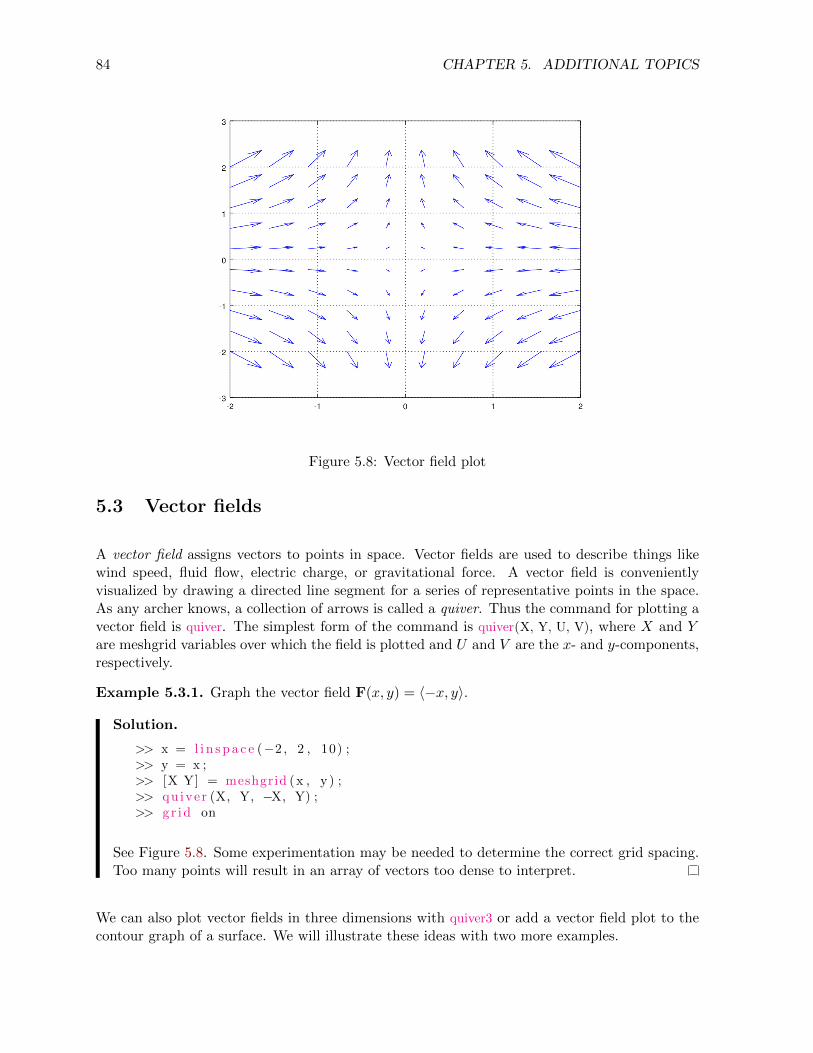
84 CHAPTER 5. ADDITIONAL TOPICS
Figure 5.8: Vector field plot
5.3 Vector fields
A vector field assigns vectors to points in space. Vector fields are used to describe things likewind speed, fluid flow, electric charge, or gravitational force. A vector field is convenientlyvisualized by drawing a directed line segment for a series of representative points in the space.As any archer knows, a collection of arrows is called a quiver. Thus the command for plotting avector field is quiver. The simplest form of the command is quiver(X, Y, U, V), where X and Yare meshgrid variables over which the field is plotted and U and V are the x- and y-components,respectively.
Example 5.3.1. Graph the vector field F(x, y) = 〈−x, y〉.
Solution.
>> x = l i n s p a c e (−2 , 2 , 10) ;>> y = x ;>> [X Y] = meshgrid (x , y ) ;>> qu iver (X, Y, −X, Y) ;>> g r id on
See Figure 5.8. Some experimentation may be needed to determine the correct grid spacing.Too many points will result in an array of vectors too dense to interpret.
We can also plot vector fields in three dimensions with quiver3 or add a vector field plot to thecontour graph of a surface. We will illustrate these ideas with two more examples.
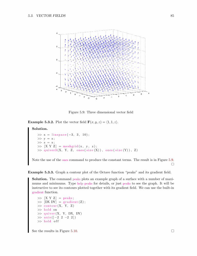
5.3. VECTOR FIELDS 85
Figure 5.9: Three dimensional vector field
Example 5.3.2. Plot the vector field F(x, y, z) = 〈1, 1, z〉.
Solution.
>> x = l i n s p a c e (−3 , 3 , 10) ;>> y = x ;>> z = x ;>> [X Y Z ] = meshgrid (x , y , z ) ;>> quiver3 (X, Y, Z , ones ( s i z e (X) ) , ones ( s i z e (Y) ) , Z)
Note the use of the ones command to produce the constant terms. The result is in Figure 5.9.
Example 5.3.3. Graph a contour plot of the Octave function “peaks” and its gradient field.
Solution. The command peaks plots an example graph of a surface with a number of maxi-mums and minimums. Type help peaks for details, or just peaks to see the graph. It will beinstructive to see its contours plotted together with its gradient field. We can use the built-ingradient function.
>> [X Y Z ] = peaks ;>> [DX DY] = grad i en t (Z) ;>> contour (X, Y, Z)>> hold on>> qu iver (X, Y, DX, DY)>> a x i s ([−2 2 −2 2 ] )>> hold o f f
See the results in Figure 5.10.
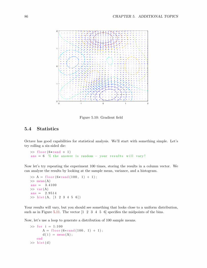
86 CHAPTER 5. ADDITIONAL TOPICS
Figure 5.10: Gradient field
5.4 Statistics
Octave has good capabilities for statistical analysis. We’ll start with something simple. Let’stry rolling a six-sided die:
>> f l o o r (6* rand + 1)ans = 6 % the answer i s random − your r e s u l t s w i l l vary !
Now let’s try repeating the experiment 100 times, storing the results in a column vector. Wecan analyze the results by looking at the sample mean, variance, and a histogram.
>> A = f l o o r (6* rand (100 , 1) + 1) ;>> mean(A)ans = 3.4100>> var (A)ans = 2.9514>> h i s t (A, [ 1 2 3 4 5 6 ] )
Your results will vary, but you should see something that looks close to a uniform distribution,such as in Figure 5.11. The vector [1 2 3 4 5 6] specifies the midpoints of the bins.
Now, let’s use a loop to generate a distribution of 100 sample means.
>> f o r i = 1:100A = f l o o r (6* rand (100 , 1) + 1) ;d ( i ) = mean(A) ;
end>> h i s t (d)
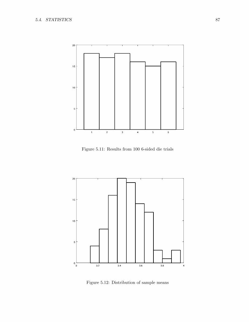
5.4. STATISTICS 87
Figure 5.11: Results from 100 6-sided die trials
Figure 5.12: Distribution of sample means
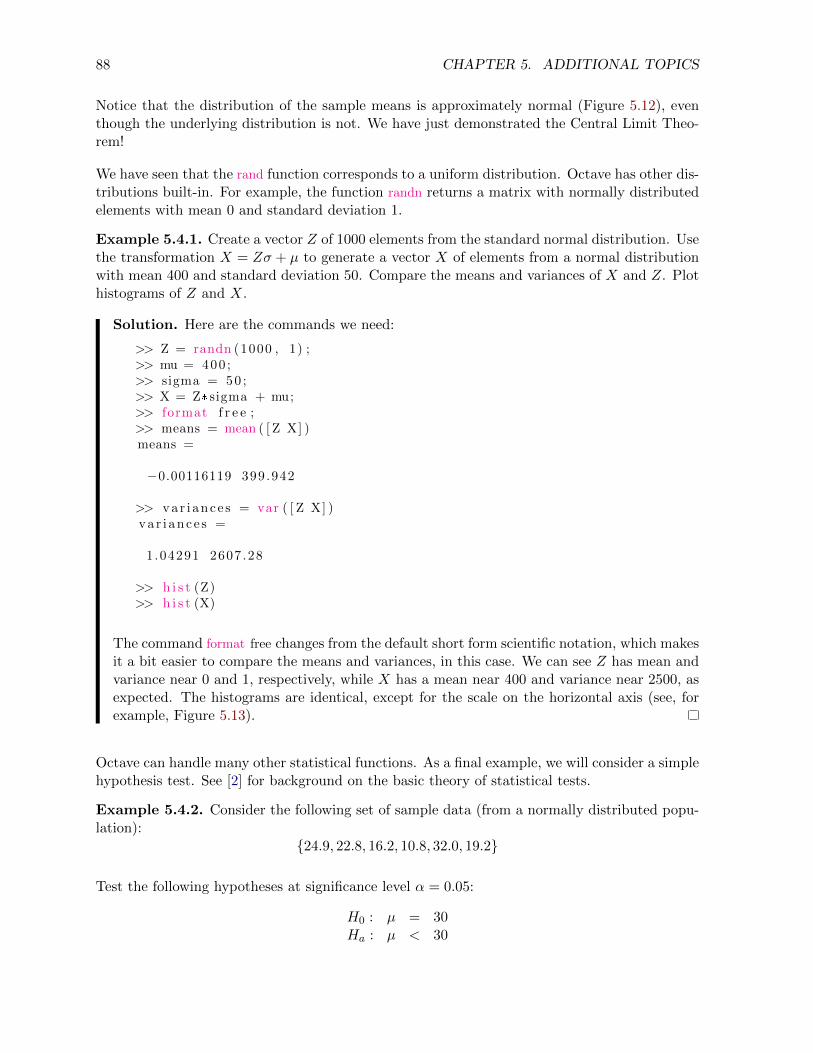
88 CHAPTER 5. ADDITIONAL TOPICS
Notice that the distribution of the sample means is approximately normal (Figure 5.12), eventhough the underlying distribution is not. We have just demonstrated the Central Limit Theo-rem!
We have seen that the rand function corresponds to a uniform distribution. Octave has other dis-tributions built-in. For example, the function randn returns a matrix with normally distributedelements with mean 0 and standard deviation 1.
Example 5.4.1. Create a vector Z of 1000 elements from the standard normal distribution. Usethe transformation X = Zσ + µ to generate a vector X of elements from a normal distributionwith mean 400 and standard deviation 50. Compare the means and variances of X and Z. Plothistograms of Z and X.
Solution. Here are the commands we need:
>> Z = randn (1000 , 1) ;>> mu = 400 ;>> sigma = 50 ;>> X = Z* sigma + mu;>> format f r e e ;>> means = mean ( [ Z X] )means =
−0.00116119 399.942
>> va r i ance s = var ( [ Z X] )va r i anc e s =
1.04291 2607.28
>> h i s t (Z)>> h i s t (X)
The command format free changes from the default short form scientific notation, which makesit a bit easier to compare the means and variances, in this case. We can see Z has mean andvariance near 0 and 1, respectively, while X has a mean near 400 and variance near 2500, asexpected. The histograms are identical, except for the scale on the horizontal axis (see, forexample, Figure 5.13).
Octave can handle many other statistical functions. As a final example, we will consider a simplehypothesis test. See [2] for background on the basic theory of statistical tests.
Example 5.4.2. Consider the following set of sample data (from a normally distributed popu-lation):
{24.9, 22.8, 16.2, 10.8, 32.0, 19.2}
Test the following hypotheses at significance level α = 0.05:
H0 : µ = 30Ha : µ < 30
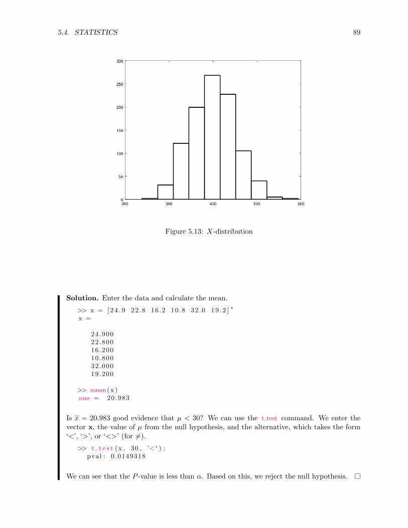
5.4. STATISTICS 89
Figure 5.13: X-distribution
Solution. Enter the data and calculate the mean.
>> x = [ 2 4 . 9 22 .8 16 .2 10 .8 32 .0 1 9 . 2 ] '
x =
24.90022 .80016 .20010 .80032 .00019 .200
>> mean( x )ans = 20.983
Is x = 20.983 good evidence that µ < 30? We can use the t test command. We enter thevector x, the value of µ from the null hypothesis, and the alternative, which takes the form‘<’, ‘>’, or ‘<>’ (for 6=).
>> t t e s t (x , 30 , '< ' ) ;pval : 0 .0149318
We can see that the P -value is less than α. Based on this, we reject the null hypothesis.
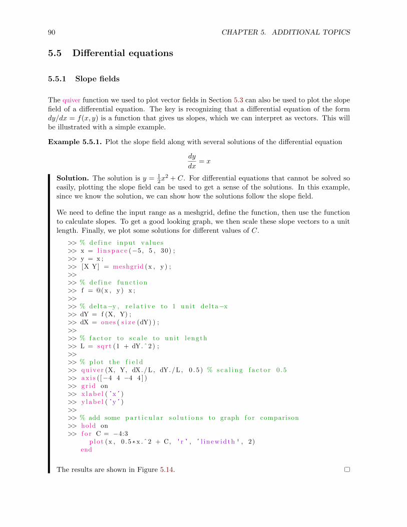
90 CHAPTER 5. ADDITIONAL TOPICS
5.5 Differential equations
5.5.1 Slope fields
The quiver function we used to plot vector fields in Section 5.3 can also be used to plot the slopefield of a differential equation. The key is recognizing that a differential equation of the formdy/dx = f(x, y) is a function that gives us slopes, which we can interpret as vectors. This willbe illustrated with a simple example.
Example 5.5.1. Plot the slope field along with several solutions of the differential equation
dy
dx= x
Solution. The solution is y = 12x
2 + C. For differential equations that cannot be solved soeasily, plotting the slope field can be used to get a sense of the solutions. In this example,since we know the solution, we can show how the solutions follow the slope field.
We need to define the input range as a meshgrid, define the function, then use the functionto calculate slopes. To get a good looking graph, we then scale these slope vectors to a unitlength. Finally, we plot some solutions for different values of C.
>> % d e f i n e input va lue s>> x = l i n s p a c e (−5 , 5 , 30) ;>> y = x ;>> [X Y] = meshgrid (x , y ) ;>>>> % d e f i n e func t i on>> f = @(x , y ) x ;>>>> % delta−y , r e l a t i v e to 1 un i t de l ta−x>> dY = f (X, Y) ;>> dX = ones ( s i z e (dY) ) ;>>>> % f a c t o r to s c a l e to un i t l ength>> L = s q r t (1 + dY. ˆ 2 ) ;>>>> % plo t the f i e l d>> qu iver (X, Y, dX. /L , dY. /L , 0 . 5 ) % s c a l i n g f a c t o r 0 .5>> a x i s ([−4 4 −4 4 ] )>> g r id on>> x l a b e l ( 'x ' )>> y l a b e l ( 'y ' )>>>> % add some p a r t i c u l a r s o l u t i o n s to graph f o r comparison>> hold on>> f o r C = −4:3
p l o t (x , 0 .5* x .ˆ2 + C, ' r ' , ' l i n ew id th ' , 2)end
The results are shown in Figure 5.14.
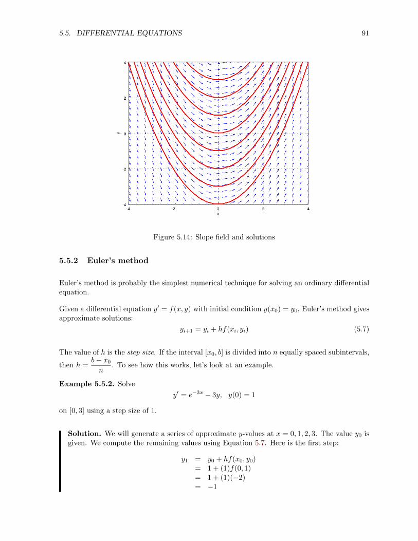
5.5. DIFFERENTIAL EQUATIONS 91
Figure 5.14: Slope field and solutions
5.5.2 Euler’s method
Euler’s method is probably the simplest numerical technique for solving an ordinary differentialequation.
Given a differential equation y′ = f(x, y) with initial condition y(x0) = y0, Euler’s method givesapproximate solutions:
yi+1 = yi + hf(xi, yi) (5.7)
The value of h is the step size. If the interval [x0, b] is divided into n equally spaced subintervals,
then h =b− x0n
. To see how this works, let’s look at an example.
Example 5.5.2. Solve
y′ = e−3x − 3y, y(0) = 1
on [0, 3] using a step size of 1.
Solution. We will generate a series of approximate y-values at x = 0, 1, 2, 3. The value y0 isgiven. We compute the remaining values using Equation 5.7. Here is the first step:
y1 = y0 + hf(x0, y0)= 1 + (1)f(0, 1)= 1 + (1)(−2)= −1
92 CHAPTER 5. ADDITIONAL TOPICS
This is then used to compute y2.
y2 = y1 + hf(x1, y1)= −1 + (1)f(1,−1)= 2.0498
One more step:y3 = y2 + hf(x2, y2)
= 2.0498 + (1)f(2, 2.0498)= −4.0971
Our approximate solutions are summarized in the following table.
x y
0 1.00001 −1.00002 2.04983 −4.0971
Unfortunately, these solutions are not very accurate. But, we can do much better by decreas-ing the step size, as shown in the next example.
These repetitive computations are best implemented in an Octave script. This allows usinga smaller step size, which gives a finer range of solution values and also improves the overallaccuracy. Refer to [7] for a fuller discussion of the accuracy of Euler’s method and a range ofmore sophisticated algorithms.
Example 5.5.3. Solve
y′ = e−3x − 3y, y(0) = 1
on [0, 3] using a step size of 0.1.
Solution. We will write a fairly general Octave script that can be easily modified for differentfunctions, intervals, and step sizes.
Octave Script 5.4: Euler’s method
1 % Euler ' s method s o l u t i o n f o r2 % dy/dx = eˆ(−3x ) − 3y , y (0 ) = 1 on [ 0 , 3 ]3
4 % d e f i n e func t i on and i n i t i a l c ond i t i on5 f = @(x , y ) exp(−3*x ) − 3*y ;6 y0 = 1 ;7
8 % d e f i n e i n t e r v a l and step s i z e9 a = 0 ;
10 b = 3 ;11 h = 0 . 1 ; % note : s tep s i z e must d iv id e b−a12 n = (b − a ) /h ;13
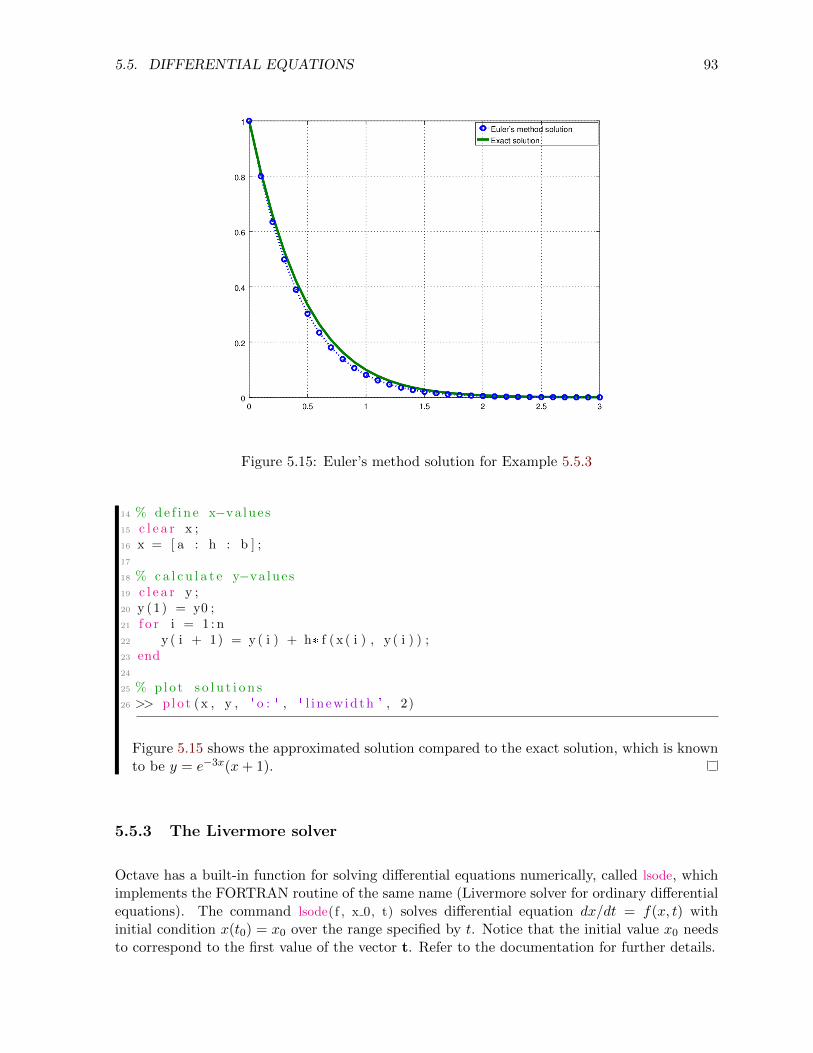
5.5. DIFFERENTIAL EQUATIONS 93
Figure 5.15: Euler’s method solution for Example 5.5.3
14 % d e f i n e x−va lue s15 c l e a r x ;16 x = [ a : h : b ] ;17
18 % c a l c u l a t e y−va lue s19 c l e a r y ;20 y (1 ) = y0 ;21 f o r i = 1 : n22 y ( i + 1) = y ( i ) + h* f ( x ( i ) , y ( i ) ) ;23 end24
25 % plo t s o l u t i o n s26 >> p lo t (x , y , ' o : ' , ' l i n ew id th ' , 2)
Figure 5.15 shows the approximated solution compared to the exact solution, which is knownto be y = e−3x(x+ 1).
5.5.3 The Livermore solver
Octave has a built-in function for solving differential equations numerically, called lsode, whichimplements the FORTRAN routine of the same name (Livermore solver for ordinary differentialequations). The command lsode(f , x 0, t) solves differential equation dx/dt = f(x, t) withinitial condition x(t0) = x0 over the range specified by t. Notice that the initial value x0 needsto correspond to the first value of the vector t. Refer to the documentation for further details.
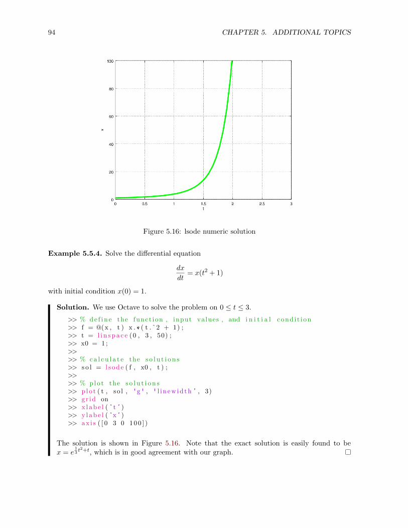
94 CHAPTER 5. ADDITIONAL TOPICS
Figure 5.16: lsode numeric solution
Example 5.5.4. Solve the differential equation
dx
dt= x(t2 + 1)
with initial condition x(0) = 1.
Solution. We use Octave to solve the problem on 0 ≤ t ≤ 3.
>> % d e f i n e the funct ion , input values , and i n i t i a l c ond i t i on>> f = @(x , t ) x . * ( t . ˆ2 + 1) ;>> t = l i n s p a c e (0 , 3 , 50) ;>> x0 = 1 ;>>>> % c a l c u l a t e the s o l u t i o n s>> s o l = l s ode ( f , x0 , t ) ;>>>> % plo t the s o l u t i o n s>> p lo t ( t , so l , ' g ' , ' l i n ew id th ' , 3)>> g r id on>> x l a b e l ( ' t ' )>> y l a b e l ( 'x ' )>> a x i s ( [ 0 3 0 1 0 0 ] )
The solution is shown in Figure 5.16. Note that the exact solution is easily found to bex = e
13t2+t, which is in good agreement with our graph.
EXERCISES 95
Chapter 5 Exercises
1. Graph the function r(t) = 〈e−t, t, sin(t)〉.
2. Graph the function f(x, y) = sin(xy) + 1.
3. Find a vector function that represents the curve of intersection of the circular cylinderx2 + y2 = 4 and the parabolic cylinder z = x2. Graph the two surfaces and the curve ofintersection.The command [X Y Z] = cylinder([2 2]) can be used to obtain a cylinder of radius 2.
4. Calculate the volume of the bumpy sphere from Example 5.1.1.
5. A cylindrical drill with radius 1 is used to bore a hole through the center of a sphere ofradius 5. Graph the ring shaped solid that remains and find its volume.
6. Use dblquad to evaluate the double integral∫∫D
x cos y dA
where D is bounded by y = 0, y = x2, and x = 2.
7. Let f(x, y) = x+2y2, defined on R = [0, 2]×[0, 4]. Write a vectorized algorithm to computea double Riemann sum using midpoints of each subrectangle as the sample points. Usea partition with m = n = 1000. Compare your results to the value computed usingdblquad('f ' , 0, 2, 0, 4) and to the estimate using upper right hand corner sample points.
8. Plot the vector field F(x, y) = tan−1( yx
)i + ln(x2)j.
9. Plot the vector field F(x, y, z) = −x(x2+y2+z2)3/2
i + −y(x2+y2+z2)3/2
j + −z(x2+y2+z2)3/2
k.
10. The function binopdf(x, n, p) gives the probability of x successes in n trials of a binomialexperiment with a probability of success p on each trial. Plot binomial distributions forn = 10, 25, and 50 with p = 0.8. This can be done with the command bar(x, B), where x isthe vector of possible outcomes and B is the corresponding vector of binomial probabilities.What happens to the shape of the distribution as n increases?
11. Use Euler’s method to solve the differential equation
dx
dt= x(t2 + 1)
with initial condition x(0) = 1 on [0, 3] using a step size h = 0.1. Compare to the lsodesolution from Example 5.5.4.
12. Graph the slope field for the logistic equationdy
dx= y(1− y). Verify that y = 1/(1 + e−x)
is a solution to the equation. Graph this function over the slope field and set the axes toan appropriate range.
13. Use lsode to solve the differential equation from Exercise 12 if y(0) = 0.5. Plot the solutionover the slope field. Does the solution agree with the previous solution?

96 CHAPTER 5. ADDITIONAL TOPICS
Appendix A
MATLAB compatibility
Octave and MATLAB use similar syntax, but the programs are not identical. MATLAB, espe-cially when extended with its various toolboxes, has many functions not available in Octave. Forexample, symbolic operations are possible, and many more options exist for solving differentialequations beyond Octave’s lsode. However, most code in this book will work in MATLAB, sowhat you’ve learned here will easily transfer to more advanced MATLAB programming.
Octave allows some flexibility in syntax that MATLAB does not. This book has been writtenwith MATLAB compatibility in mind, so when multiple forms of a command or operation arepossible, the MATLAB compatible option has been used. Here is a summary of a few of thepotential coding differences.
� Comments in Octave can be preceded by # or %. MATLAB uses %.
� Octave recognizes single quotes and double quotes around strings. MATLAB requiressingle quotes.
� Blocks in Octave can be ended with end statements based on the initial command (endfor,endfunction, etc). MATLAB uses only end.
� The not-equal comparison can be written as != or ˜= in Octave. MATLAB uses ˜=.
� Octave allows user-defined functions to be entered at the command line or in scripts.MATLAB requires the use of separate function files.
� The lsode command is not implemented in MATLAB. There are many other options avail-able, such as ode45. To use ode45 and several other MATLAB compatible solvers in Octave,load the package ‘odepkg.’
97

98 APPENDIX A. MATLAB COMPATIBILITY
Appendix B
List of Octave commands
The names and basic syntax for many common commands are provided below. Type help NAME
at the Octave prompt for more details.
List of Octave commands
Syntax Description
[a:step:b] . . . . . . . . . . . . . . . . . . . . . vector from a to b by increment ‘step’
A' . . . . . . . . . . . . . . . . . . . . . . . . . . . . transpose of A
A*B . . . . . . . . . . . . . . . . . . . . . . . . . . matrix product A×BA\b . . . . . . . . . . . . . . . . . . . . . . . . . . . left division, solves system Ax = b
Aˆn . . . . . . . . . . . . . . . . . . . . . . . . . . . matrix power
A + B . . . . . . . . . . . . . . . . . . . . . . . . sum A+B
x < y . . . . . . . . . . . . . . . . . . . . . . . . . less than comparison
x > y . . . . . . . . . . . . . . . . . . . . . . . . . greater than comparison
x == y . . . . . . . . . . . . . . . . . . . . . . . equality comparison
x ˜= y . . . . . . . . . . . . . . . . . . . . . . . . not equal comparison
x.*y . . . . . . . . . . . . . . . . . . . . . . . . . . elementwise product
x./y . . . . . . . . . . . . . . . . . . . . . . . . . . elementwise quotient
x.ˆn . . . . . . . . . . . . . . . . . . . . . . . . . . elementwise exponent
abs(x) . . . . . . . . . . . . . . . . . . . . . . . . . absolute value of x
acos(x) . . . . . . . . . . . . . . . . . . . . . . . . inverse cosine of x in radians
and(a, b) . . . . . . . . . . . . . . . . . . . . . . logical AND
ans . . . . . . . . . . . . . . . . . . . . . . . . . . . result of last calculation
asin(x) . . . . . . . . . . . . . . . . . . . . . . . . inverse sine of x in radians
atan(x) . . . . . . . . . . . . . . . . . . . . . . . . inverse tangent of x in radians
axis ([Xmin Xmax Ymin Ymax]) set axis limits
bar(x, y) . . . . . . . . . . . . . . . . . . . . . . bar graph of y vs. x
besselj (n, x) . . . . . . . . . . . . . . . . . . order n Bessel functions of the first kind
binopdf(x, n, p) . . . . . . . . . . . . . . . binomial probability of x successes
ceil (x) . . . . . . . . . . . . . . . . . . . . . . . . dxe, the least integer greater than or equal to x
clear var1 . . . . . . . . . . . . . . . . . . . . . clear variable (clear all if no variable listed)
clf . . . . . . . . . . . . . . . . . . . . . . . . . . . . clear plot window
contour(X, Y, Z) . . . . . . . . . . . . . . . contour plot of surface
corr(x, y) . . . . . . . . . . . . . . . . . . . . . linear correlation coefficient r
cos(x) . . . . . . . . . . . . . . . . . . . . . . . . . cosine of x (x in radians)
cosh(x) . . . . . . . . . . . . . . . . . . . . . . . . hyperbolic cosine of x
cross(u, v) . . . . . . . . . . . . . . . . . . . . cross product of vectors u and v
cylinder ([ r r ]) . . . . . . . . . . . . . . . . cylinder of radius r
dblquad('f ' , a, b, c, d) . . . . . . . . double integral over rectangle
continued . . .
99
100 APPENDIX B. LIST OF OCTAVE COMMANDS
. . . continued
Syntax Description
det(A) . . . . . . . . . . . . . . . . . . . . . . . . determinant of A
dir . . . . . . . . . . . . . . . . . . . . . . . . . . . . list files in current directory
dot(u, v) . . . . . . . . . . . . . . . . . . . . . . dot product of vectors u and v
[v lambda] = eig(A) . . . . . . . . . . . . find eigenvalues and eigenvectors
e . . . . . . . . . . . . . . . . . . . . . . . . . . . . . the number e
erf (x) . . . . . . . . . . . . . . . . . . . . . . . . . the error function
exp(x) . . . . . . . . . . . . . . . . . . . . . . . . natural exponential function
eye(n) . . . . . . . . . . . . . . . . . . . . . . . . . n× n identity matrix
floor (x) . . . . . . . . . . . . . . . . . . . . . . . bxc, the greatest integer less than or equal to x
for i = 1:n ... end . . . . . . . . . . . . for loop
format opt . . . . . . . . . . . . . . . . . . . . . decimal format, options = short, long, free, bank, etc
fsolve ( ' f ' , x1) . . . . . . . . . . . . . . . . solve f(x) = 0, initial guess x1function y = f(x) ... end . . . . . . . define a function
f = @(x1, x2, ...) rule . . . . . . . . . anonymous function of x1, x2, . . . given by rule
[DX DY] = gradient(Z) . . . . . . . . . gradient field of Z
gamma(x) . . . . . . . . . . . . . . . . . . . . . the gamma function
grid on/off . . . . . . . . . . . . . . . . . . . . toggle plot grid
help NAME . . . . . . . . . . . . . . . . . . . get documentation for command ‘NAME’
hist (X, B) . . . . . . . . . . . . . . . . . . . . . histogram of X, optional B specifies bins
hold on/off . . . . . . . . . . . . . . . . . . . . add to current plot toggle on/off
I . . . . . . . . . . . . . . . . . . . . . . . . . . . . . the imaginary unit
im = imread('name') . . . . . . . . . . . load image
imagesc(A) . . . . . . . . . . . . . . . . . . . . display matrix as scaled image
imresize(im, factor) . . . . . . . . . . . . scale image by factor
imshow(im) . . . . . . . . . . . . . . . . . . . . display image
inv(A) . . . . . . . . . . . . . . . . . . . . . . . . inverse of matrix A
legend('plot1 ' , 'plot2 ' , ...) . . . plot legend
linspace(a, b, n) . . . . . . . . . . . . . . vector of n evenly spaced points from a to b
load filename . . . . . . . . . . . . . . . . . . load saved variables
log(x) . . . . . . . . . . . . . . . . . . . . . . . . . natural logarithm
lsode(f , x 0, t) . . . . . . . . . . . . . . . solves dx/dt = f(x, t), x(0) = x0[L U P] = lu(A) . . . . . . . . . . . . . . . LU decomposition of A, with permutation
max(A) . . . . . . . . . . . . . . . . . . . . . . . maximum of vector, or column-wise maximums of a matrix
max(max(A)) . . . . . . . . . . . . . . . . . . maximum of all entries in matrix A
mean(x) . . . . . . . . . . . . . . . . . . . . . . . mean of x
mesh(X, Y, Z) . . . . . . . . . . . . . . . . . surface plotted as a mesh
[X Y] = meshgrid(x, y) . . . . . . . . . generate X,Y -meshgrid
min(A) . . . . . . . . . . . . . . . . . . . . . . . . minimum of vector, or column-wise minimums of a matrix
min(min(A)) . . . . . . . . . . . . . . . . . . . minimum of all entries in matrix A
norm(u) . . . . . . . . . . . . . . . . . . . . . . . norm (length) of vector u
normcdf(x, mu, sigma) . . . . . . . . . . area under normal curve to the left of x
norminv(a, mu, sigma) . . . . . . . . . . inverse normal distribution given area a
ones(m, n) . . . . . . . . . . . . . . . . . . . . . m× n matrix of ones
continued . . .
101
. . . continued
Syntax Description
or(a, b) . . . . . . . . . . . . . . . . . . . . . . . logical OR
peaks . . . . . . . . . . . . . . . . . . . . . . . . . example 3d graph of a surface with many local extrema
pi . . . . . . . . . . . . . . . . . . . . . . . . . . . . the number π
pinv(A) . . . . . . . . . . . . . . . . . . . . . . . pseudoinverse of A
pkg install −forge NAME . . . . . . download and install a package from Octave Forge
pkg list . . . . . . . . . . . . . . . . . . . . . . . list installed packages
pkg load NAME . . . . . . . . . . . . . . . load an installed package
plot(x, y) . . . . . . . . . . . . . . . . . . . . . plot of x vs. y
plot3(x, y, z) . . . . . . . . . . . . . . . . . plot space curve
polyfit (x, y, order) . . . . . . . . . . . . polynomial fit x vs. y of degree ‘order’
polyval(P, x) . . . . . . . . . . . . . . . . . . evaluate polynomial P at x
print −dpng filename.png . . . . . . save plot as png (substitute jpg, eps, etc)
pwd . . . . . . . . . . . . . . . . . . . . . . . . . . . list current working directory
[Q R] = qr(A) . . . . . . . . . . . . . . . . . QR decomposition of A
quad('f ' , a, b) . . . . . . . . . . . . . . . . definite integral
quiver(X, Y, U, V) . . . . . . . . . . . . . plot vector field with components U and V
quiver3(X, Y, Z, U, V, W) . . . . . . plot 3d vector field with components U, V, W
rand(m, n) . . . . . . . . . . . . . . . . . . . . m× n random matrix (uniformly distributed entries)
randn(m, n) . . . . . . . . . . . . . . . . . . . m× n random matrix (normally distributed entries)
rank(A) . . . . . . . . . . . . . . . . . . . . . . . rank of A
rgb2gray(im) . . . . . . . . . . . . . . . . . . convert image to grayscale
save filename A, B, ... . . . . . . . . . save variables A, B, ...
sin(x) . . . . . . . . . . . . . . . . . . . . . . . . . sine of x (x in radians)
sinh(x) . . . . . . . . . . . . . . . . . . . . . . . . hyperbolic sine of x
size (A, opt) . . . . . . . . . . . . . . . . . . . dimensions of A; dimension option: 1=rows, 2=cols
sqrt(x) . . . . . . . . . . . . . . . . . . . . . . . . principle square root of x
sum(A) . . . . . . . . . . . . . . . . . . . . . . . sum of vector components or column-wise sum of matrix A
sum(sum(A)) . . . . . . . . . . . . . . . . . . sum of all entries in matrix A
surf(X, Y, Z) . . . . . . . . . . . . . . . . . . surface plot
[U S V] = svd(A) . . . . . . . . . . . . . . singular value decomposition of A
tcdf(x, n) . . . . . . . . . . . . . . . . . . . . . Students t-distribution CDF with degrees of freedom n
tinv(a, n) . . . . . . . . . . . . . . . . . . . . . inverse t-distribution with degrees of freedom n
t test (X, mu 0, alt) . . . . . . . . . . . . t-test, alternative hypothesis = ‘<’,‘>’, or ‘<>’
tan(x) . . . . . . . . . . . . . . . . . . . . . . . . . tangent of x (x in radians)
tanh(x) . . . . . . . . . . . . . . . . . . . . . . . hyperbolic tangent of x
title ( 'name') . . . . . . . . . . . . . . . . . . assign plot title
triplequad( ' f ' , a, b, c, d, e, f) triple integral over a rectangular box
var(x) . . . . . . . . . . . . . . . . . . . . . . . . . variance of x
whos . . . . . . . . . . . . . . . . . . . . . . . . . . list variables in current scope
xlabel( 'name') . . . . . . . . . . . . . . . . . horizontal axis label
ylabel( 'name') . . . . . . . . . . . . . . . . . vertical axis label
zeros(m, n) . . . . . . . . . . . . . . . . . . . . m× n matrix of zeros

102 APPENDIX B. LIST OF OCTAVE COMMANDS
References
[1] Brin, Leon Q, Tea Time Numerical Analysis, 2nd edition. CC-BY-SA, 2016.http://lqbrin.github.io/tea-time-numerical/
[2] Diez, David M, Christopher D Barr, and Mine Cetinkaya-Rundel, OpenIntro Statistics, 3rdedition. CC-BY-SA, 2015.https://www.openintro.org/stat/textbook.php
[3] Eaton, John W, David Bateman, Søren Hauberg, and Rik Wehbring, GNU Octave Manual:Edition 4. GNU FDL, 2017.https://www.gnu.org/software/octave/octave.pdf
[4] Grinstead, Charles M, and J Laurie Snell, Introduction to Probability, 2nd Edition.American Mathematical Society. GNU FDL, 2006.http://www.dartmouth.edu/~chance/teaching_aids/books_articles/probability_
book/book.html
[5] Kuttler, Ken, A First Course in Linear Algebra. CC-BY, 2017.http://lyryx.com/textbooks/Kuttler-LinearAlgebra-AFirstCourse-2017A.pdf
[6] Strang, Gilbert, Edwin Herman, et al, Calculus Volumes 1–3. OpenStax. CC-BY-NC-SA,2016.https://openstax.org/details/books/calculus-volume-1
https://openstax.org/details/books/calculus-volume-2
https://openstax.org/details/books/calculus-volume-3
[7] Trench, William F, Elementary Differential Equations. Trinity University, Digital Com-mons. CC-BY-NC-SA, 2013.http://digitalcommons.trinity.edu/mono/8/
103

104 REFERENCES
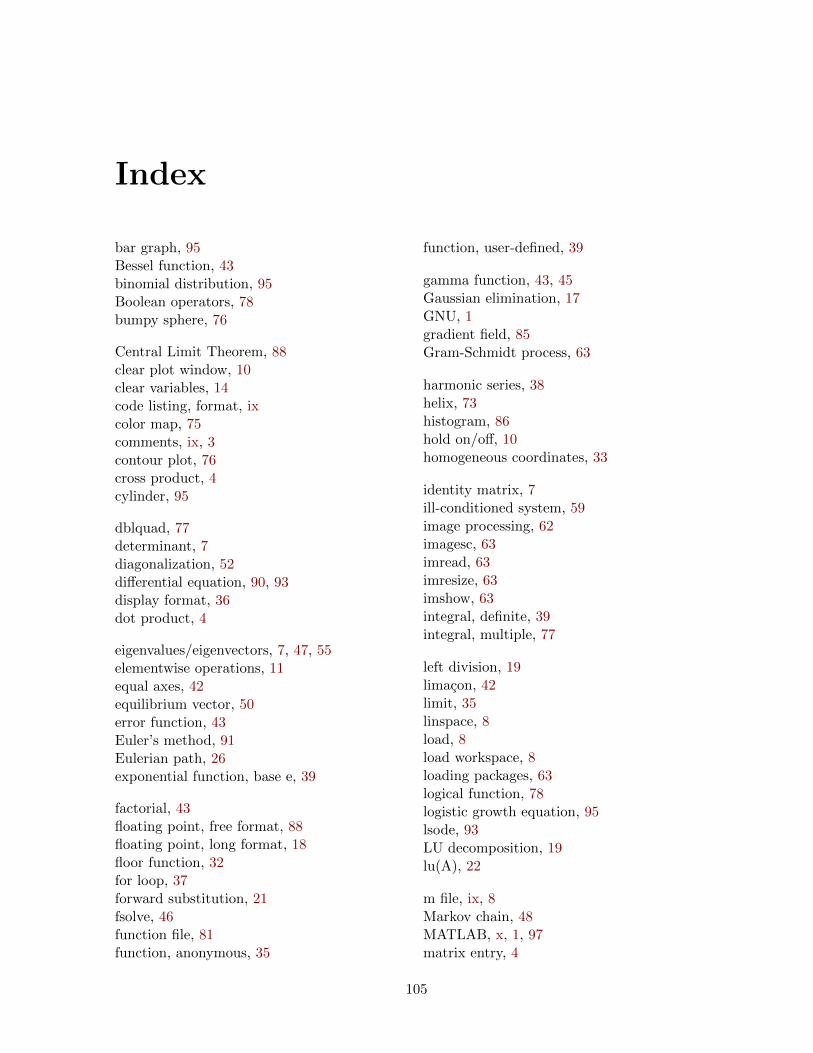
Index
bar graph, 95Bessel function, 43binomial distribution, 95Boolean operators, 78bumpy sphere, 76
Central Limit Theorem, 88clear plot window, 10clear variables, 14code listing, format, ixcolor map, 75comments, ix, 3contour plot, 76cross product, 4cylinder, 95
dblquad, 77determinant, 7diagonalization, 52differential equation, 90, 93display format, 36dot product, 4
eigenvalues/eigenvectors, 7, 47, 55elementwise operations, 11equal axes, 42equilibrium vector, 50error function, 43Euler’s method, 91Eulerian path, 26exponential function, base e, 39
factorial, 43floating point, free format, 88floating point, long format, 18floor function, 32for loop, 37forward substitution, 21fsolve, 46function file, 81function, anonymous, 35
function, user-defined, 39
gamma function, 43, 45Gaussian elimination, 17GNU, 1gradient field, 85Gram-Schmidt process, 63
harmonic series, 38helix, 73histogram, 86hold on/off, 10homogeneous coordinates, 33
identity matrix, 7ill-conditioned system, 59image processing, 62imagesc, 63imread, 63imresize, 63imshow, 63integral, definite, 39integral, multiple, 77
left division, 19limacon, 42limit, 35linspace, 8load, 8load workspace, 8loading packages, 63logical function, 78logistic growth equation, 95lsode, 93LU decomposition, 19lu(A), 22
m file, ix, 8Markov chain, 48MATLAB, x, 1, 97matrix entry, 4
105
106 INDEX
matrix indexing, 17matrix inverse, 7matrix multiplication, 6mean, 86mesh, 76meshgrid, 75midpoint rule, 39
natural logarithm, 33nested loops, 82Newton’s method, 46nonrectangular domain, 78norm, 4normal distribution, standard, 88normal equations, 24numerical integration, 38, 77
Octave script, ix, 8, 40Octave, graphical user interface, 2Octave, installation, 2ones, 24, 85orthogonal diagonalization, 54orthogonal matrix, 54orthonormal set, 63
parametric surface, 76partial sums, sequence of, 37peaks, 85permutation matrix, 22plot, 9plot options, 10, 12plot3, 73plotting points, 10polar coordinates, 42polyfit, 25polyval, 26printing to file, 13probability vector, 49projection, scalar, 5projection, vector, 5, 64pseudoinverse, 59
QR algorithm, 67QR decomposition, 65qr(A), 67quad, 39quadrature (definite integral), 39quiver, 84, 90quiver3, 84
random matrix, 31rank, 7rgb2gray, 63Riemann sum, 82rotation matrix, 27rref, 18
save, 8save workspace, 8semi-log plot, 33sequence, 37Simpson’s rule, 39singular value decomposition, 56singular values, 56slope field, 90solid of revolution, 76space curve, 73special functions, 43string variables, ixsurf, 75surface, 75svd, 59symmetric matrix, 54
transition matrix, 49transpose, 7trapezoid rule, 39triplequad, 77
uniform distribution, 86
variable assignment, 3variance, 86vector field, 84vectorized code, 35, 82

Cover image: Mandelbrot Set, created with GNU Octave by the author.
These notes are intended to provide a brief, noncomprehensive introduction to GNU Octave, a free open source alternative to MatLab. The basic syntax and usage is explained through concrete examples from the mathematics courses a math, computer science, or engineering major encounters in the first two years of college: linear algebra, calculus, and differential equations.
Copyright 2017 by Jason Lachniet.
This work is licensed under a Creative Commons Attribution-ShareAlike 4.0 International License.