Introduction to GeneticAnalysis

Ecology and Evolutionary Biology,University of Arizona

Adjunct Appointments Molecular and Cellular Biology

Plant SciencesEpidemiology & Biostatistics

Animal Sciences

Bruce Walsh

jbwalsh@u.arizona.edu

Outline• Mendelian Genetics

– Genes, Chromosomes & DNA– Mendel’s laws– Linkage– Linkage disequilibrium

• Quantitative Genetics– Fisher’s decomposition of Genetic value– Fisher decomposition of Genetic Variances– Resemblance between relatives– Searching for the underlying genes

Mendelian Genetics

Following a single (or several) genes that we can directly

score

Phenotype highly informative as to genotype

Mendel’s GenesGenes are discrete particles, with each parent passingone copy to its offspring.

Let an allele be a particular copy of a gene. In Diploids,each parent carries two alleles for every gene, onefrom each parent

Each parent contributes one of its two alleles (atrandom) to its offspring

For example, a parent with genotype Aa (a heterozygote for alleles A and a) has a 50% probability of passing anA allele onto its offspring and a 50% probability ofpassing along an a allele.

Example: Pea seed color

Mendel found that his pea lines differed in seed color,with a single locus (with alleles Y and g) determining green vs. yellow

YY (Y homozygote) --> yellow phenotypeYg (heterozygote) --> yellow phenotypegg (g homozygote) --> green phenotype

Note that in this simple case, each genotype mapsto a single phenotype

Likewise, the phenotype can tell us about the underlyingGenotype. Green = gg, Yellow = carries Y allele

Y is dominant to g, g is recessive to Y

Cross Yg x Yg. Offspring are 1/4 YY, 1/2 Yg, 1/4 gg3/4 yellow peas, 1/4 green peas

Cross Yg x gg. Offspring are 1/2Yg, 1/2 gg,1/2 yellow, 1/2 green

Dealing with two (or more) genes

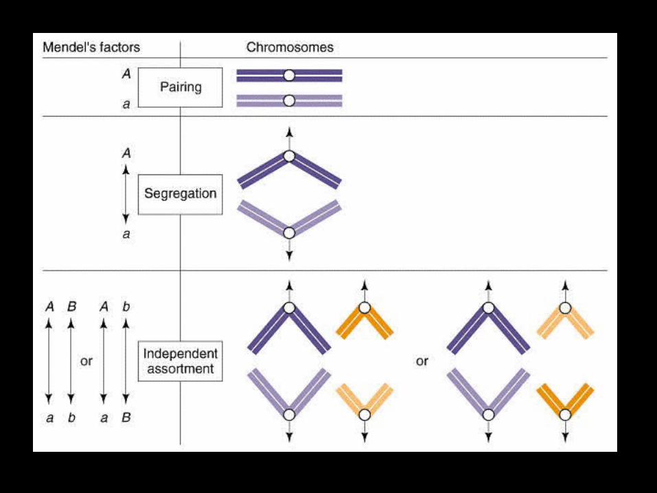
For 7 pea traits, Mendel observed Independent Assortment

The genotype at one locus is independent of the second

RR, Rr - round seeds, rr - wrinkled seeds

Pure round, green (RRgg) x pure wrinkled yellow (rrYY)

F1 --> RrYg = all round, yellow

What about the F2?

YY, Yg - yellow seeds, gg - green seeds

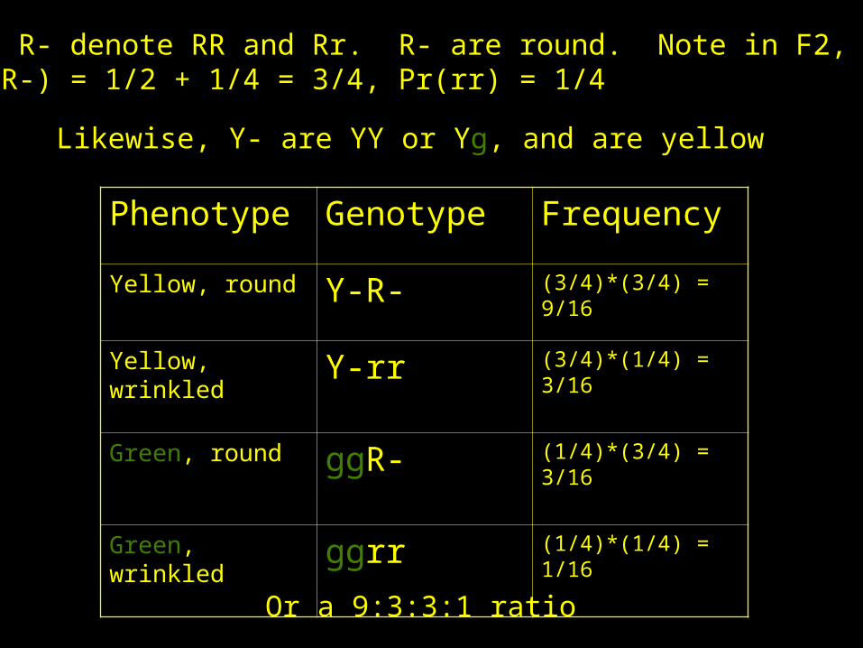
Let R- denote RR and Rr. R- are round. Note in F2,Pr(R-) = 1/2 + 1/4 = 3/4, Pr(rr) = 1/4

Likewise, Y- are YY or Yg, and are yellow

Phenotype Genotype Frequency

Yellow, round Y-R- (3/4)*(3/4) = 9/16

Yellow, wrinkled Y-rr (3/4)*(1/4) = 3/16

Green, round ggR- (1/4)*(3/4) = 3/16

Green, wrinkled ggrr (1/4)*(1/4) = 1/16

Or a 9:3:3:1 ratio

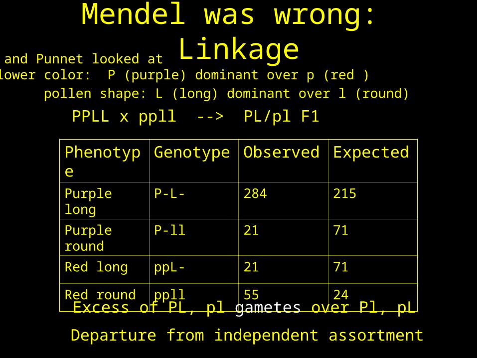
Mendel was wrong: Linkage

Phenotype

Genotype Observed Expected

Purple long P-L- 284 215

Purple round

P-ll 21 71

Red long ppL- 21 71

Red round ppll 55 24

Bateson and Punnet looked at flower color: P (purple) dominant over p (red )

pollen shape: L (long) dominant over l (round)

Excess of PL, pl gametes over Pl, pL

Departure from independent assortment

PPLL x ppll --> PL/pl F1

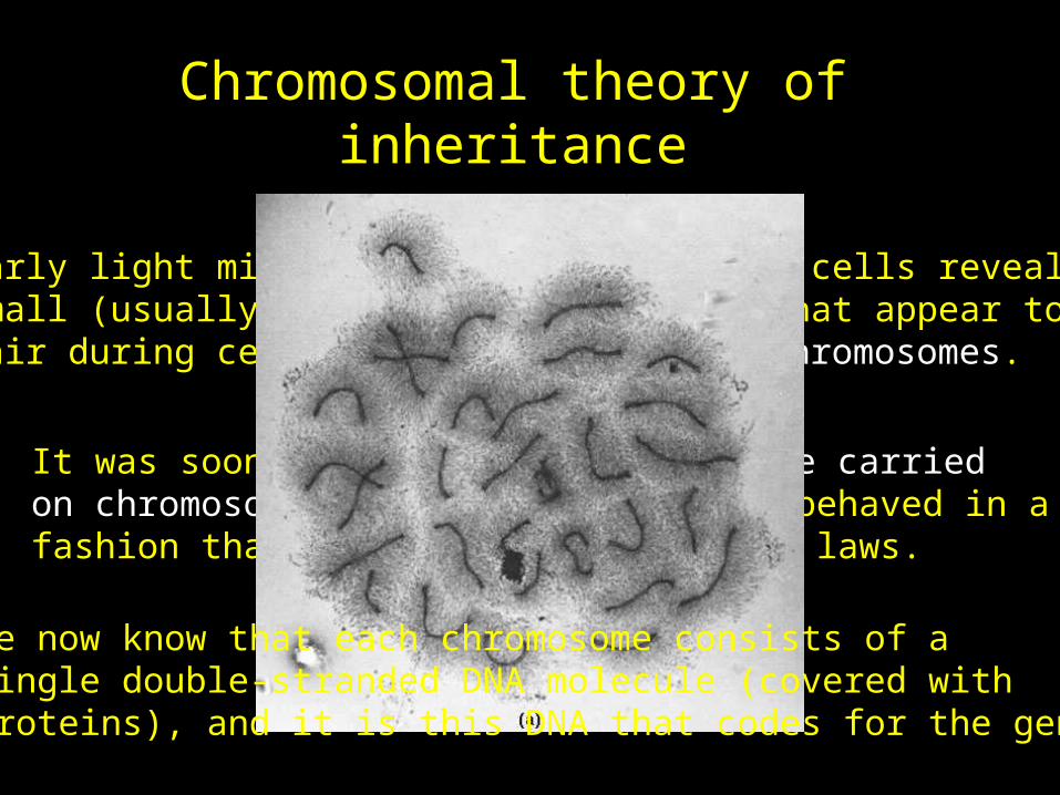
Chromosomal theory of inheritance

It was soon postulated that Genes are carried on chromosomes, because chromosomes behaved in afashion that would generate Mendel’s laws.

Early light microscope work on dividing cells revealedsmall (usually) rod-shaped structures that appear topair during cell division. These are chromosomes.

We now know that each chromosome consists of asingle double-stranded DNA molecule (covered withproteins), and it is this DNA that codes for the genes.

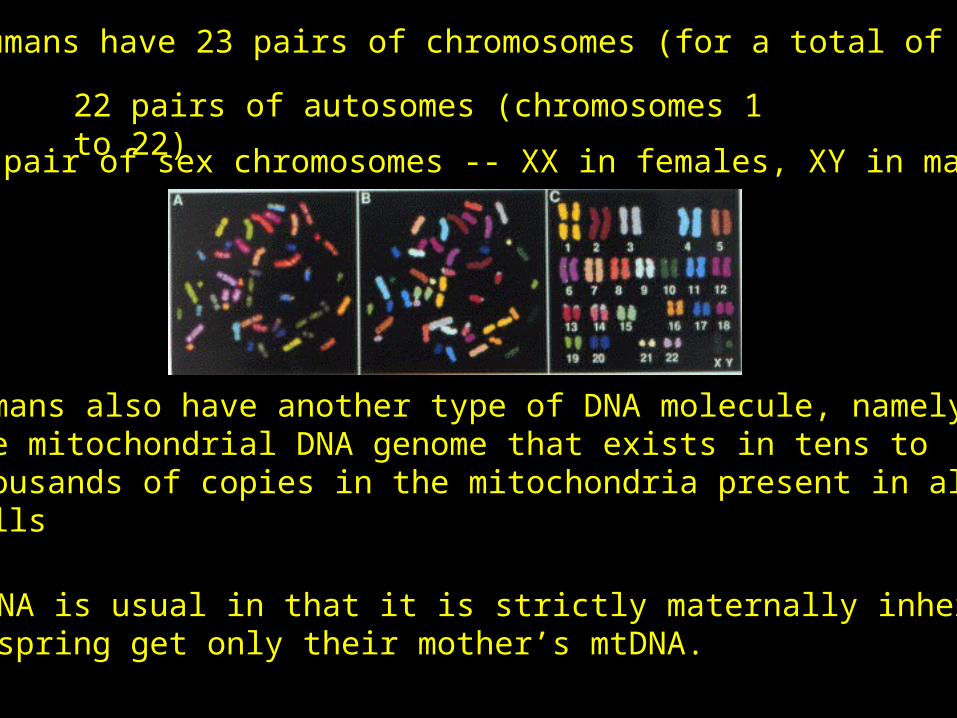
Humans have 23 pairs of chromosomes (for a total of 46)

22 pairs of autosomes (chromosomes 1 to 22)1 pair of sex chromosomes -- XX in females, XY in males

Humans also have another type of DNA molecule, namelythe mitochondrial DNA genome that exists in tens to thousands of copies in the mitochondria present in all ourcells

mtDNA is usual in that it is strictly maternally inherited.Offspring get only their mother’s mtDNA.

Linkage

If genes are located on different chromosomes they(with very few exceptions) show independent assortment.

Indeed, peas have only 7 chromosomes, so was Mendel luckyin choosing seven traits at random that happen to allbe on different chromosomes? Problem: compute this probability.

However, genes on the same chromosome, especially ifthey are close to each other, tend to be passed ontotheir offspring in the same configuation as on theparental chromosomes.

Consider the Bateson-Punnet pea data

Let PL / pl denote that in the parent, one chromosomecarries the P and L alleles (at the flower color andpollen shape loci, respectively), while the other chromosome carries the p and l alleles.

Unless there is a recombination event, one of the twoparental chromosome types (PL or pl) are passed ontothe offspring. These are called the parental gametes.

However, if a recombination event occurs, a PL/pl parent can generate Pl and pL recombinant gametesto pass onto its offspring.

Linkage --> excess of parental gametes

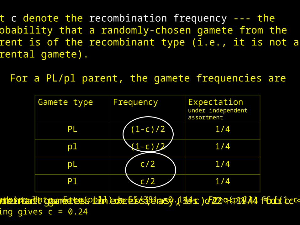
Let c denote the recombination frequency --- theprobability that a randomly-chosen gamete from theparent is of the recombinant type (i.e., it is not aparental gamete).

For a PL/pl parent, the gamete frequencies are

Gamete type Frequency Expectation under independent assortment

PL (1-c)/2 1/4

pl (1-c)/2 1/4

pL c/2 1/4

Pl c/2 1/4

Parental gametes in excess, as (1-c)/2 > 1/4 for c < 1/2Recombinant gametes in deficiency, as c/2 < 1/4 for c < 1/2In Bateson data, Freq(ppll) = 55/381 =0.144. Freq(ppll) = [(1-c)/2]2,Solving gives c = 0.24

Linkage is our friendWhile linkage (at first blush) may seem a complication, itis actually our friend, allowing us to map genes --- determining which genes are on which chromosomes and also fine-mapping their position on a particular chromosome

Historically, the genes that have been mapped havedirect effects on phenotypes (pea color, fly eye color,any number of simple human diseases, etc. )

In the molecular era, we are often concerned withmolecular markers, variations in the DNA sequence thattypically have no effect on phenotype

Molecular MarkersYou and your neighbor differ at roughly 22,000,000 nucleotides (base pairs) out of the roughly 3 billionbp that comprises the human genome

Hence, LOTS of molecular variation to exploit

SNP -- single nucleotide polymorphism. A particularposition on the DNA (say base 123,321 on chromosome 1)that has two different nucleotides (say G or A) segregating

STR -- simple tandem arrays. An STR locus consists ofa number of short repeats, with alleles defined bythe number of repeats. For example, you might have6 and 4 copies of the repeat on your two chromsome 2s

Gametes and Gamete Frequencies

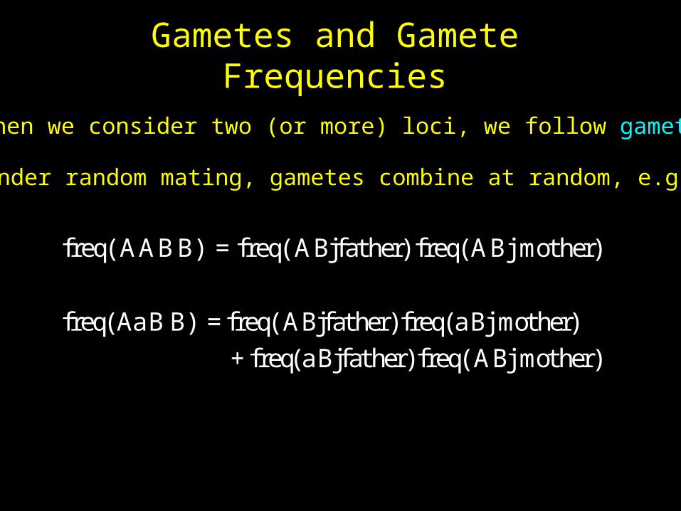
freq(AABB) = freq(ABjfather) freq(ABjmother)

freq(AaBB) =freq(ABjfather)freq(aBjmother)+freq(aBjfather)freq(ABjmother)

When we consider two (or more) loci, we follow gametes

Under random mating, gametes combine at random, e.g.

Linkage disequilibrium

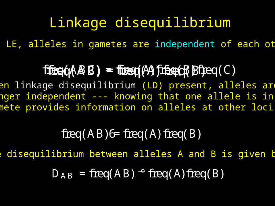
freq(AB) = freq(A) freq(B)freq(ABC) = freq(A)freq(B)freq(C)

At LE, alleles in gametes are independent of each other:

When linkage disequilibrium (LD) present, alleles are nolonger independent --- knowing that one allele is in the gamete provides information on alleles at other loci

freq(AB)6= freq(A) freq(B)

The disequilibrium between alleles A and B is given by

DA B = freq(AB) ° freq(A)freq(B)

Forces that Generate LD

• Selection• Drift• Migration (admixture)• Mutation• Population structure (stratification)

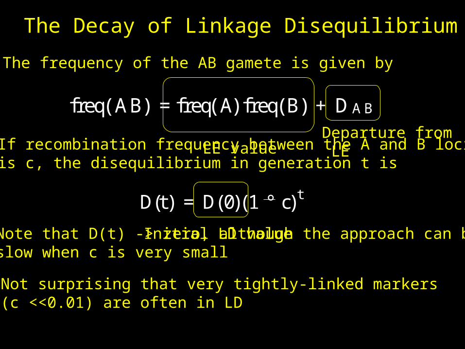
freq(AB) = freq(A) freq(B) + DAB

D(t) = D(0)(1 c)t°

The Decay of Linkage Disequilibrium

The frequency of the AB gamete is given by

LE valueDeparture from LEIf recombination frequency between the A and B loci

is c, the disequilibrium in generation t is

Initial LD valueNote that D(t) -> zero, although the approach can beslow when c is very small

Not surprising that very tightly-linked markers (c <<0.01) are often in LD

Key Mendelian Concepts• Genes, Chromosomes & DNA• “Classical” vs Molecular markers• Linkage

– Parental gametes in excess. Alleles at nearby loci tend to segregate together

• Linkage disequilibrium (LD)– Excess of parental gametes seen in any particular

cross– LD implies in the population that there is a non-

random association of allele– Unlinked alleles can show LD due to population

structure

Quantitative Genetics

The analysis of traits whose variation is determined by

both a number of genes and environmental factors

Phenotype is highly uninformative as tounderlying genotype

Complex (or Quantitative) trait

• No (apparent) simple Mendelian basis for variation in the trait

• May be a single gene strongly influenced by environmental factors

• May be the result of a number of genes of equal (or differing) effect

• Most likely, a combination of both multiple genes and environmental factors.

• Example: Blood pressure, cholesterol levels– Known genetic and environmental risk factors

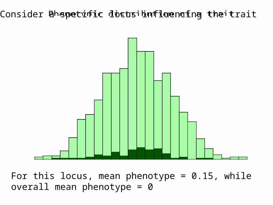
Phenotypic distribution of a traitConsider a specific locus influencing the trait

For this locus, mean phenotype = 0.15, whileoverall mean phenotype = 0

Goals of Quantitative Genetics

• Partition total trait variation into genetic (nature) vs. environmental (nurture) components

• Predict resemblance between relatives– If a sib has a disease/trait, what are your odds?

• Find the underlying loci contributing to genetic variation – QTL -- quantitative trait loci

• Deduce molecular basis for genetic trait variation

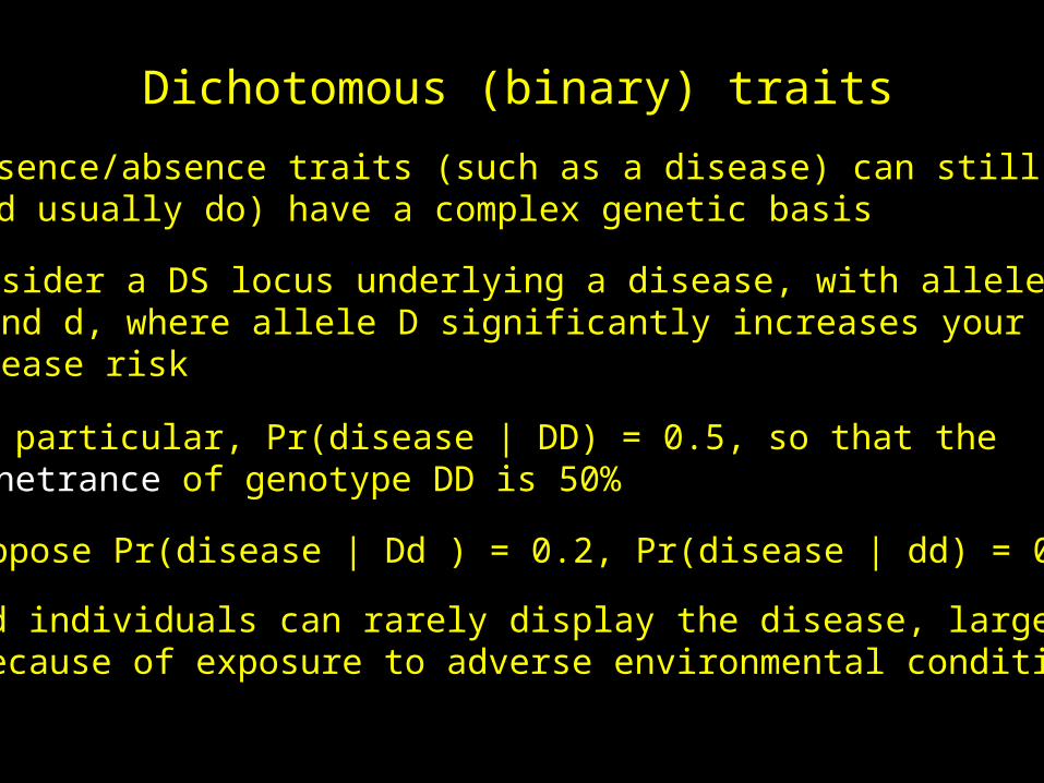
Dichotomous (binary) traits

Presence/absence traits (such as a disease) can still(and usually do) have a complex genetic basis

Consider a DS locus underlying a disease, with allelesD and d, where allele D significantly increases yourdisease risk

In particular, Pr(disease | DD) = 0.5, so that thePenetrance of genotype DD is 50%

Suppose Pr(disease | Dd ) = 0.2, Pr(disease | dd) = 0.05

dd individuals can rarely display the disease, largelybecause of exposure to adverse environmental conditions

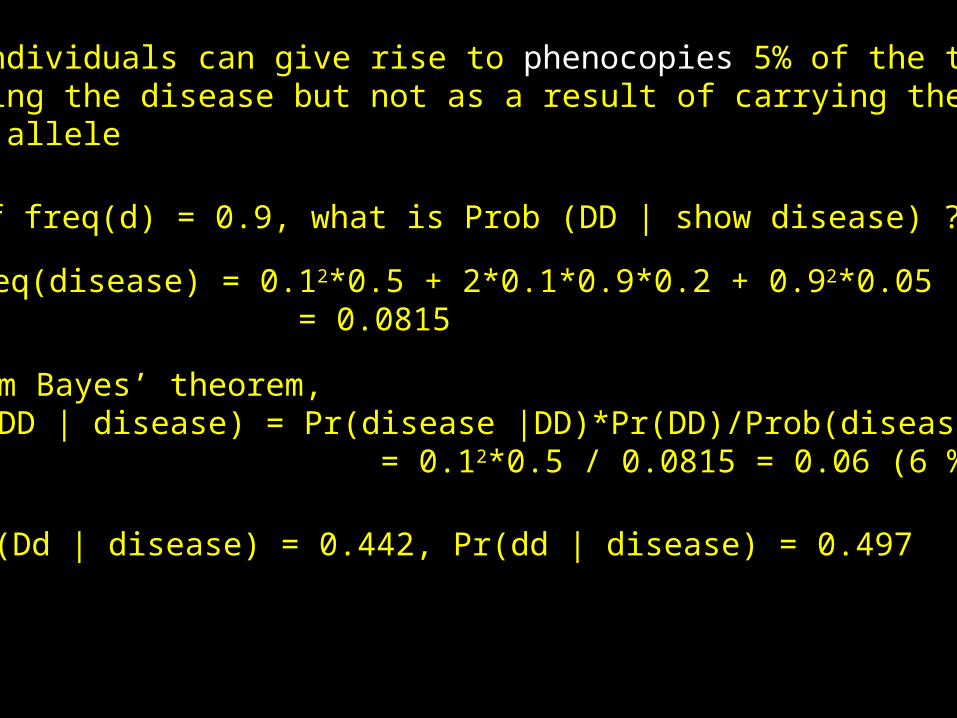
If freq(d) = 0.9, what is Prob (DD | show disease) ?

freq(disease) = 0.12*0.5 + 2*0.1*0.9*0.2 + 0.92*0.05 = 0.0815

From Bayes’ theorem, Pr(DD | disease) = Pr(disease |DD)*Pr(DD)/Prob(disease) = 0.12*0.5 / 0.0815 = 0.06 (6 %)

dd individuals can give rise to phenocopies 5% of the time,showing the disease but not as a result of carrying therisk allele

Pr(Dd | disease) = 0.442, Pr(dd | disease) = 0.497

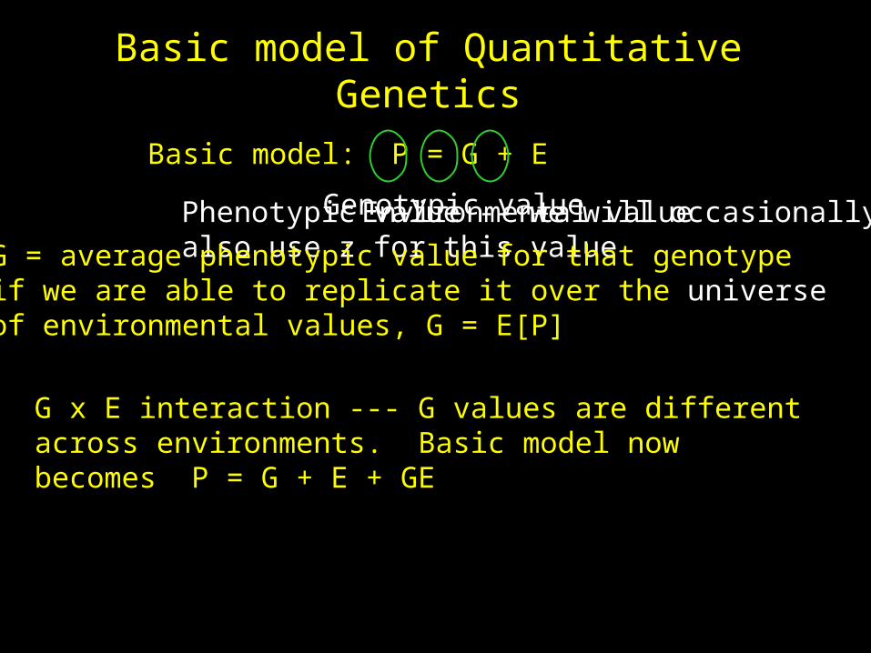
Basic model of Quantitative Genetics

Basic model: P = G + E

Phenotypic value -- we will occasionallyalso use z for this value

Genotypic valueEnvironmental value

G = average phenotypic value for that genotypeif we are able to replicate it over the universeof environmental values, G = E[P]

G x E interaction --- G values are differentacross environments. Basic model nowbecomes P = G + E + GE

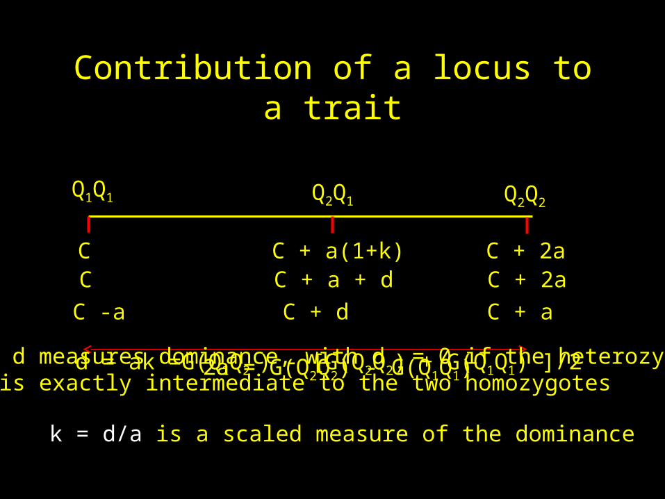
Q1Q1 Q2Q1 Q2Q2

C C + a(1+k) C + 2aC C + a + d C + 2aC -a C + d C + a

2a = G(Q2Q2) - G(Q1Q1) d = ak =G(Q1Q2 ) - [G(Q2Q2) + G(Q1Q1) ]/2 d measures dominance, with d = 0 if the heterozygoteis exactly intermediate to the two homozygotes

k = d/a is a scaled measure of the dominance

Contribution of a locus to a trait

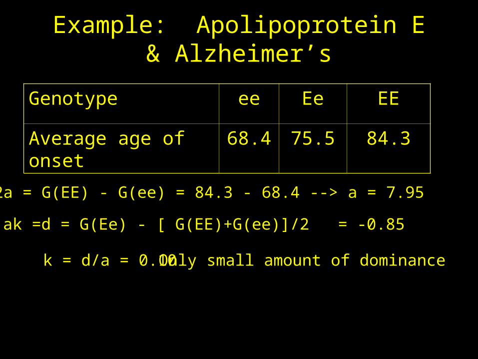
Example: Apolipoprotein E & Alzheimer’s

Genotype ee Ee EE

Average age of onset

68.4 75.5 84.3

2a = G(EE) - G(ee) = 84.3 - 68.4 --> a = 7.95

ak =d = G(Ee) - [ G(EE)+G(ee)]/2 = -0.85

k = d/a = 0.10 Only small amount of dominance

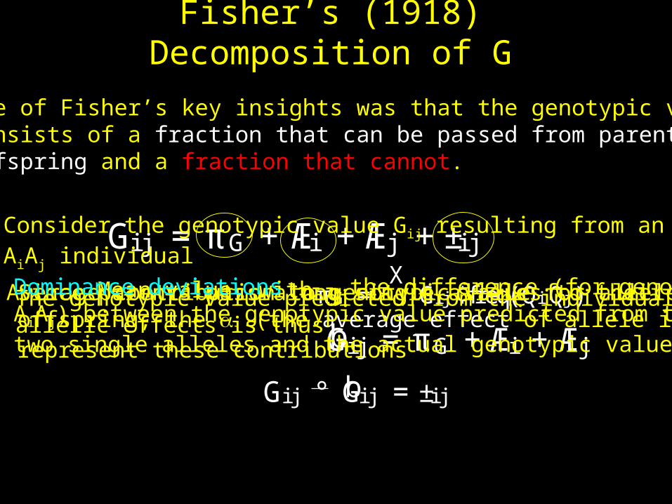
Fisher’s (1918) Decomposition of G

One of Fisher’s key insights was that the genotypic valueconsists of a fraction that can be passed from parent tooffspring and a fraction that cannot.

πG =X

Gi j ¢freq(QiQj )Mean value, withAverage contribution to genotypic value for allele iSince parents pass along single alleles to theiroffspring, the i (the average effect of allele i)represent these contributions

Gi j = πG +Æi +Æj +±i j

bGi j = πG +Æi +Æj

The genotypic value predicted from the individualallelic effects is thus

G i j ° Gi j =±i jb

Dominance deviations --- the difference (for genotypeAiAj) between the genotypic value predicted from thetwo single alleles and the actual genotypic value,

Consider the genotypic value Gij resulting from an AiAj individual

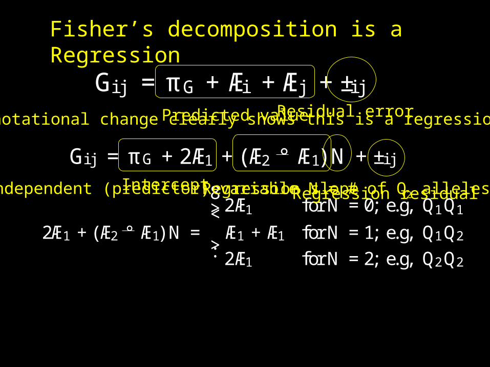
Gi j = πG +2Æ1 + (Æ2 ° Æ1)N +±i j

2Æ1 + (Æ2 ° Æ1)N =

8><

>:

2Æ1 forN =0; e.g, Q1Q1

Æ1 +Æ1 forN =1; e.g, Q1Q2

2Æ1 forN =2; e.g, Q2Q2

Gi j = πG +Æi +Æj +±i j

Fisher’s decomposition is a Regression

Predicted valueResidual errorA notational change clearly shows this is a regression,

Independent (predictor) variable N = # of Q2 allelesRegression slopeIntercept Regression residual

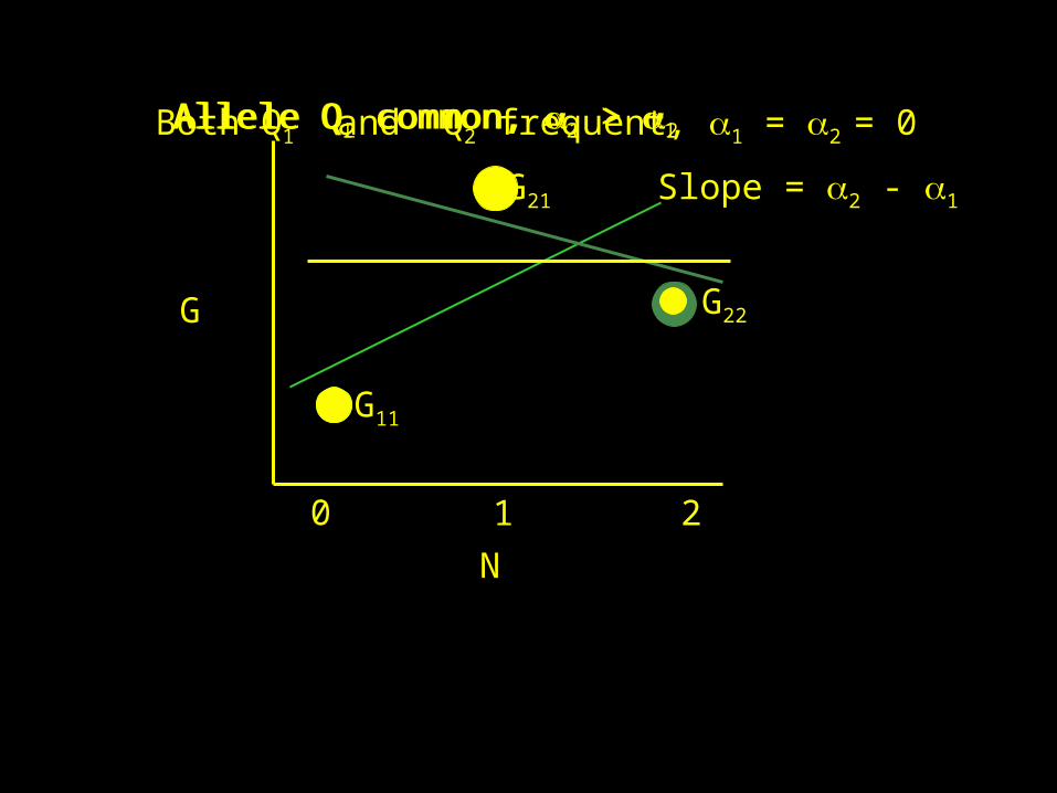
0 1 2

N

G G22

G11

G21

Allele Q1 common, 2 > 1

Slope = 2 - 1

Allele Q2 common, 1 > 2Both Q1 and Q2 frequent, 1 = 2 = 0

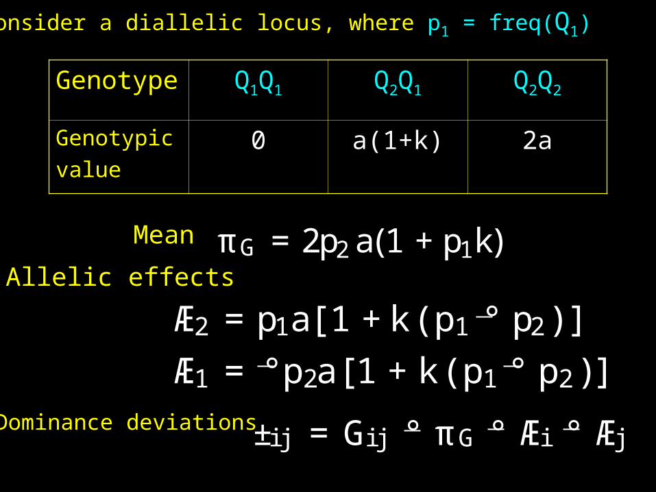
Genotype Q1Q1 Q2Q1 Q2Q2

Genotypicvalue

0 a(1+k) 2a

Consider a diallelic locus, where p1 = freq(Q1)

πG = 2p2a(1+p1k)Mean

Allelic effects

Æ2 = p1a[1+k (p1 ° p2 ) ]

Æ1 = °p2a[1+ k (p1 ° p2 )]Dominance deviations±i j = G i j ° πG ° Æi ° Æj

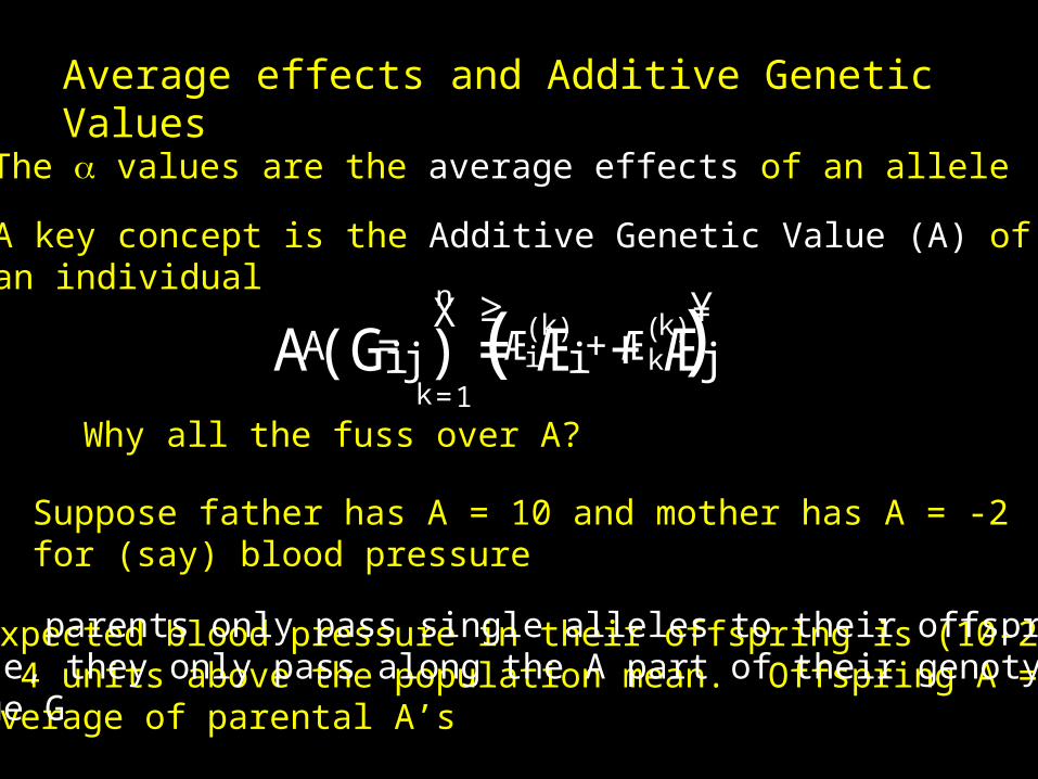
Average effects and Additive Genetic Values

A (Gi j ) =Æi +ÆjA =nX

k=1

≥Æ(k)

i +Æ(k)k

¥( )

The values are the average effects of an allele

A key concept is the Additive Genetic Value (A) ofan individual

Why all the fuss over A?

Suppose father has A = 10 and mother has A = -2for (say) blood pressure

Expected blood pressure in their offspring is (10-2)/2 = 4 units above the population mean. Offspring A =Average of parental A’s

KEY: parents only pass single alleles to their offspring.Hence, they only pass along the A part of their genotypicValue G

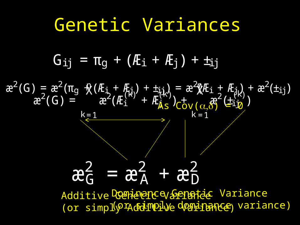
Genetic Variances

Gi j = πg + (Æi +Æj ) +±i j

æ2(G) =nX

k=1

æ2(Æ(k)i +Æ(k)

j ) +nX

k=1

æ2(±(k)i j )

æ2G =æ2

A +æ2D

æ2(G) =æ2(πg +(Æi +Æj ) +±i j ) =æ2(Æi +Æj ) +æ2(±i j)

As Cov() = 0

Additive Genetic Variance(or simply Additive Variance)

Dominance Genetic Variance(or simply dominance variance)

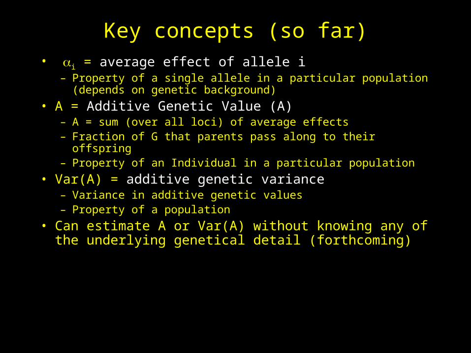
Key concepts (so far)• i = average effect of allele i

– Property of a single allele in a particular population (depends on genetic background)

• A = Additive Genetic Value (A) – A = sum (over all loci) of average effects– Fraction of G that parents pass along to their offspring– Property of an Individual in a particular population

• Var(A) = additive genetic variance– Variance in additive genetic values– Property of a population

• Can estimate A or Var(A) without knowing any of the underlying genetical detail (forthcoming)

æ2D = 2E[±2] =

mX

i=1

mX

j=1

±2i j pi pj

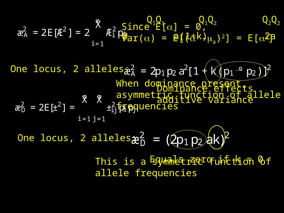
æ2D = (2p1p2 ak)2

æ2A = 2p1p2 a2[1+k (p1 ° p2 ) ]2One locus, 2 alleles:

One locus, 2 alleles:

Q1Q1 Q1Q2 Q2Q2

0 a(1+k) 2a

Dominance effects additive variance

When dominance present, asymmetric function of allele frequencies

Equals zero if k = 0This is a symmetric function ofallele frequencies

æ2A =2E[Æ2 ] = 2

mX

i=1

Æ2i pi

Since E[] = 0, Var() = E[( -a)2] = E[2]

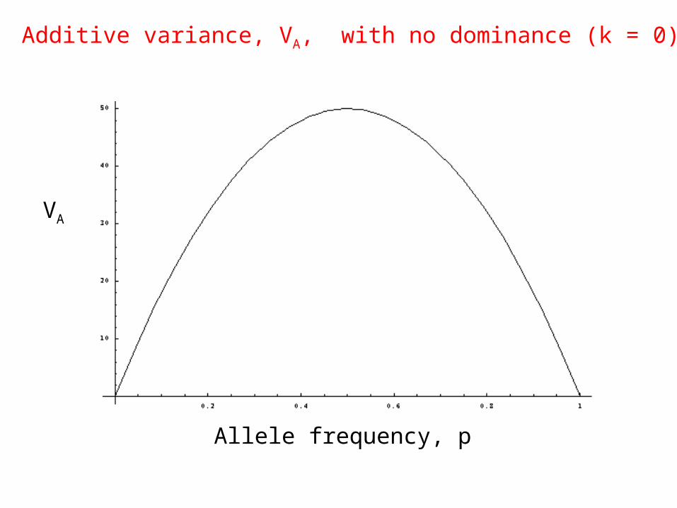
Additive variance, VA, with no dominance (k = 0)

Allele frequency, p

VA

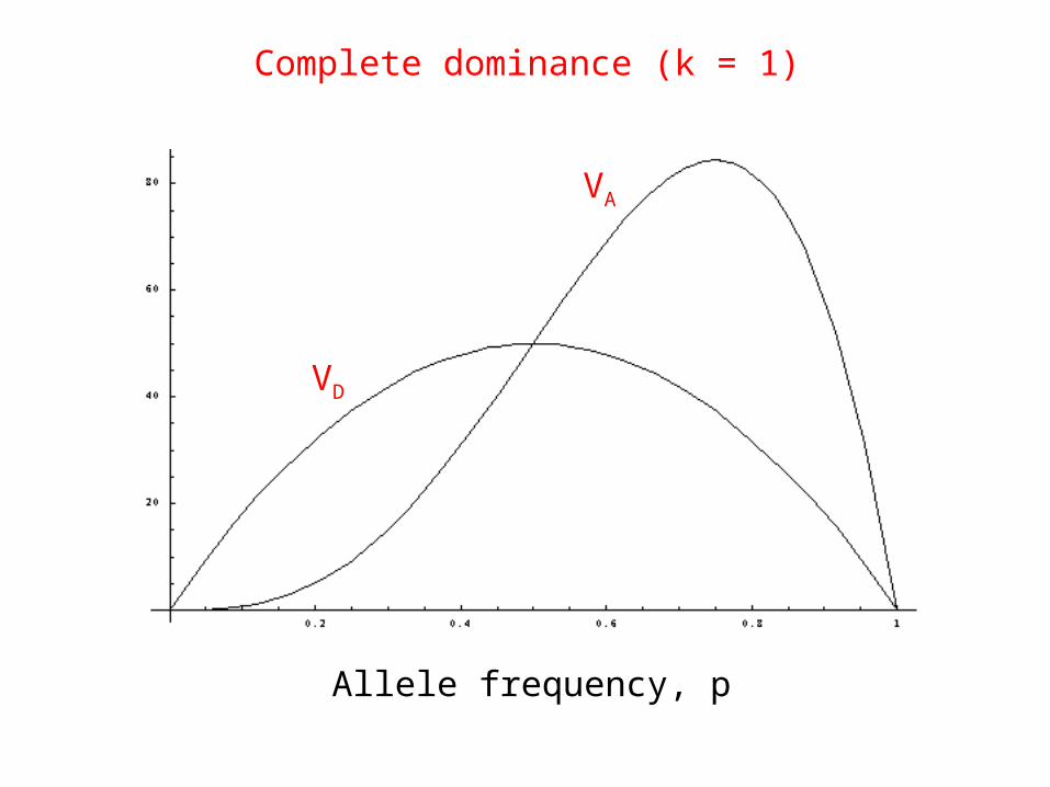
Complete dominance (k = 1)

Allele frequency, p

VA

VD

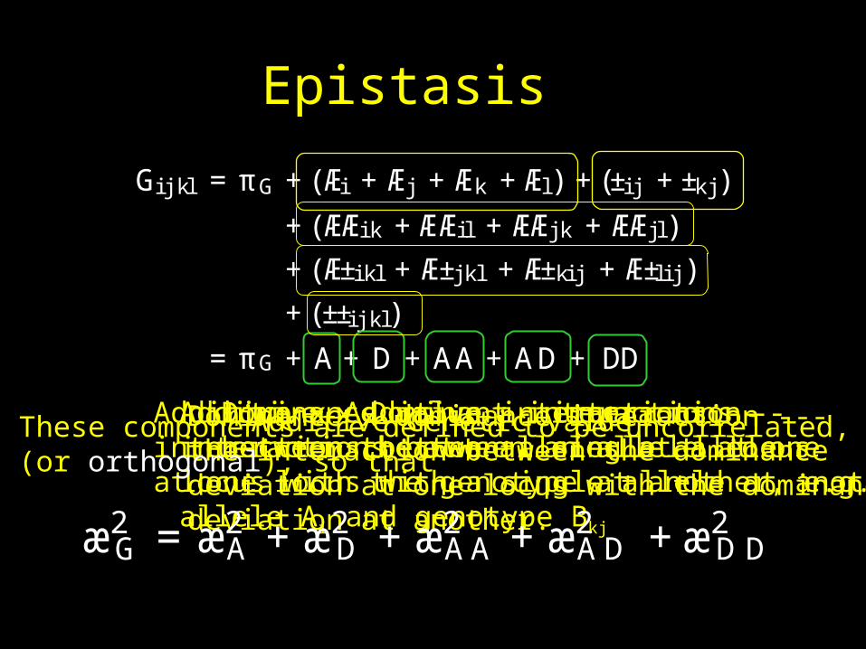
Epistasis

Gi j kl = πG + (Æi +Æj +Æk +Æl) + (±i j +±k j )

+ (ÆÆik +ÆÆi l +ÆÆjk +ÆÆj l)+ (Ʊikl +Ʊjkl +Ʊki j +Ʊl i j )+ (±±i j kl)

= πG + A + D + AA + AD + DD

Additive Genetic valueDominance value -- interactionbetween the two alleles at a locus

Additive x Additive interactions --interactions between a single alleleat one locus with a single allele at another

Additive x Dominant interactions --interactions between an allele at onelocus with the genotype at another, e.g.allele Ai and genotype Bkj

Dominance x dominance interaction ---the interaction between the dominancedeviation at one locus with the dominancedeviation at another.

These components are defined to be uncorrelated,(or orthogonal), so that

æ2G =æ2

A +æ2D +æ2

AA +æ2AD +æ2

D D

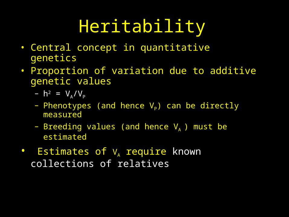
Heritability• Central concept in quantitative genetics• Proportion of variation due to additive genetic

values – h2 = VA/VP

– Phenotypes (and hence VP) can be directly measured

– Breeding values (and hence VA ) must be estimated

• Estimates of VA require known collections of relatives

Key observations

• The amount of phenotypic resemblance among relatives for the trait provides an indication of the amount of genetic variation for the trait.

• If trait variation has a significant genetic basis, the closer the relatives, the more similar their appearance

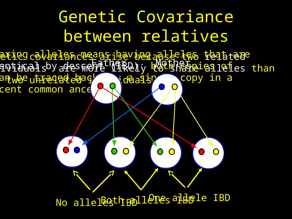
Genetic Covariance between relatives

Genetic covariances arise because two related individuals are more likely to share alleles than are two unrelated individuals.

Sharing alleles means having alleles that are identical by descent (IBD): both copies of can be traced back to a single copy in a recent common ancestor.

Father Mother

No alleles IBD One allele IBDBoth alleles IBD

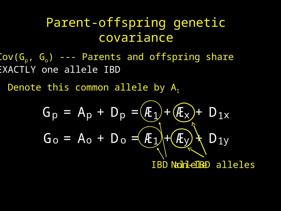
Parent-offspring genetic covariance

Cov(Gp, Go) --- Parents and offspring share EXACTLY one allele IBD

Denote this common allele by A1

Gp = Ap + Dp =Æ1 +Æx + D1x

Go = Ao + Do =Æ1 +Æy + D1y

IBD alleleNon-IBD alleles

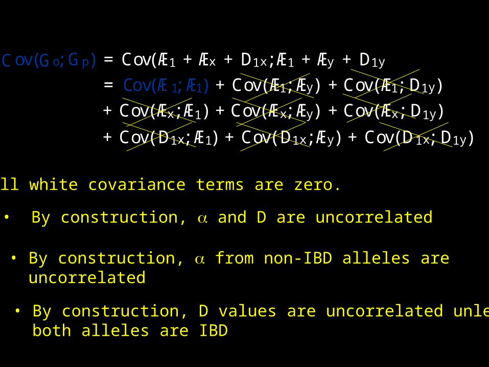
Cov(Go;Gp) = Cov(Æ1 +Æx + D1x;Æ1 +Æy + D1y

= Cov(Æ1;Æ1) + Cov(Æ1;Æy) +Cov(Æ1; D1y)+ Cov(Æx;Æ1) +Cov(Æx;Æy) +Cov(Æx; D1y)

+ Cov(D1x;Æ1) + Cov(D1x;Æy) + Cov(D1x; D1y)

All white covariance terms are zero.

• By construction, and D are uncorrelated

• By construction, from non-IBD alleles are uncorrelated

• By construction, D values are uncorrelated unless both alleles are IBD

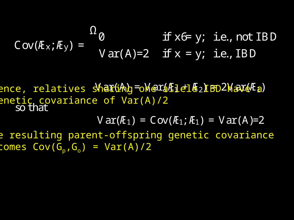
Cov(Æx;Æy) =Ω0 if x6=y; i.e., not IBD

Var(A)=2 if x =y; i.e., IBD

Var(A) = Var(Æ1 +Æ2) = 2Var(Æ1)

so thatVar(Æ1) = Cov(Æ1;Æ1) = Var(A)=2

Hence, relatives sharing one allele IBD have agenetic covariance of Var(A)/2

The resulting parent-offspring genetic covariance becomes Cov(Gp,Go) = Var(A)/2

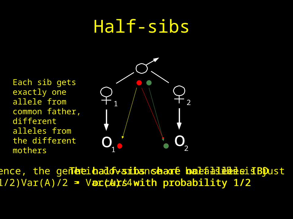
Half-sibs

The half-sibs share one allele IBD • occurs with probability 1/2

1

o1

2

o2

The half-sibs share no alleles IBD • occurs with probability 1/2

Each sib gets exactly one allele from common father,different alleles from the different mothers

Hence, the genetic covariance of half-sibs is just (1/2)Var(A)/2 = Var(A)/4

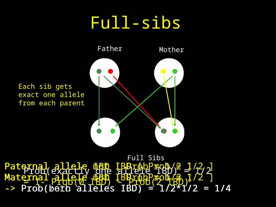
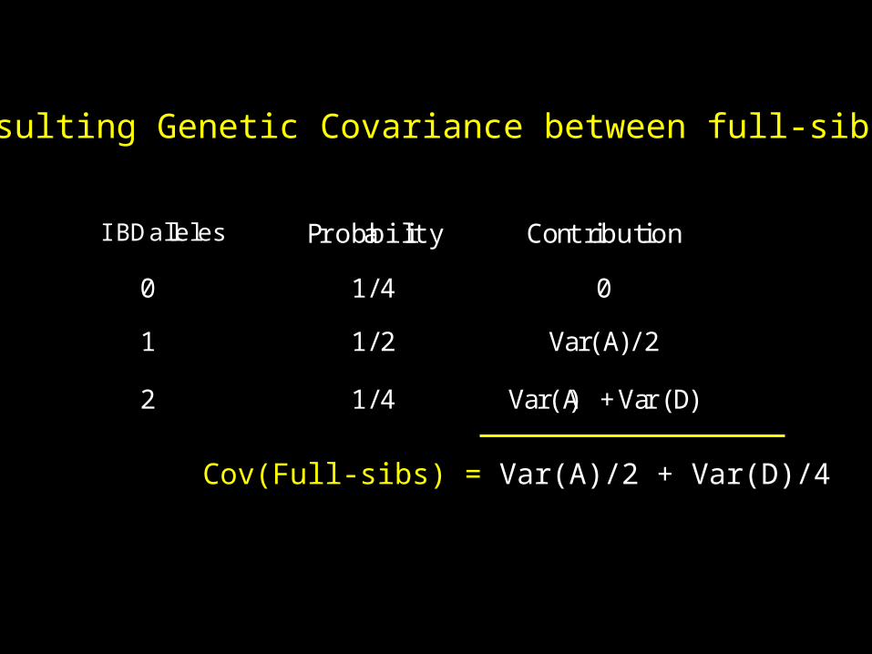
Full-sibsFather Mother

Full SibsPaternal allele not IBD [ Prob = 1/2 ]Maternal allele not IBD [ Prob = 1/2 ]-> Prob(zero alleles IBD) = 1/2*1/2 = 1/4

Paternal allele IBD [ Prob = 1/2 ]Maternal allele IBD [ Prob = 1/2 ]-> Prob(both alleles IBD) = 1/2*1/2 = 1/4

Prob(exactly one allele IBD) = 1/2= 1- Prob(0 IBD) - Prob(2 IBD)

Each sib getsexact one allelefrom each parent

IB D alleles Probability Contr ibution

0 1/ 4 0

1 1/ 2 Var(A)/ 2

2 1/ 4 Var(A) + Var(D)

IBD alleles Probability Contribution

0 1/4 0

1 1/2 Var(A)/2

2 1/4 Var(A) + Var(D)

Resulting Genetic Covariance between full-sibs

Cov(Full-sibs) = Var(A)/2 + Var(D)/4

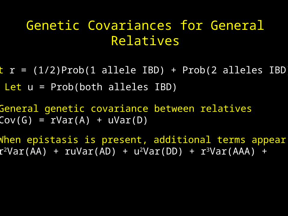
Genetic Covariances for General Relatives

Let r = (1/2)Prob(1 allele IBD) + Prob(2 alleles IBD)

Let u = Prob(both alleles IBD)

General genetic covariance between relativesCov(G) = rVar(A) + uVar(D)

When epistasis is present, additional terms appearr2Var(AA) + ruVar(AD) + u2Var(DD) + r3Var(AAA) +

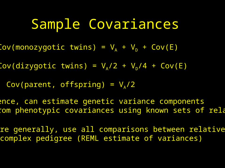
Sample Covariances

Cov(monozygotic twins) = VA + VD + Cov(E)

Cov(dizygotic twins) = VA/2 + VD/4 + Cov(E)

Cov(parent, offspring) = VA/2

Hence, can estimate genetic variance componentsFrom phenotypic covariances using known sets of relatives

More generally, use all comparisons between relatives ina complex pedigree (REML estimate of variances)

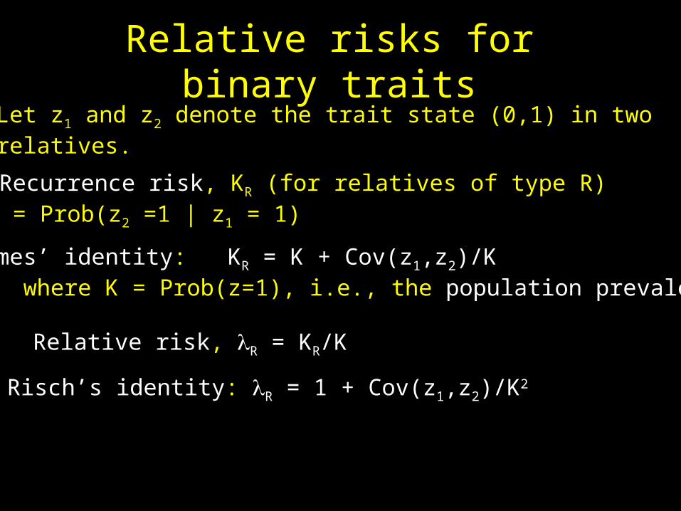
Relative risks for binary traitsLet z1 and z2 denote the trait state (0,1) in tworelatives.

Recurrence risk, KR (for relatives of type R) = Prob(z2 =1 | z1 = 1)

James’ identity: KR = K + Cov(z1,z2)/K where K = Prob(z=1), i.e., the population prevalence

Relative risk, R = KR/K

Risch’s identity: R = 1 + Cov(z1,z2)/K2

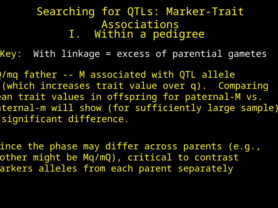
Searching for QTLs: Marker-Trait Associations

Key: With linkage = excess of parential gametes

MQ/mq father -- M associated with QTL alleleQ (which increases trait value over q). Comparingmean trait values in offspring for paternal-M vs. paternal-m will show (for sufficiently large sample) a significant difference.

Since the phase may differ across parents (e.g.,mother might be Mq/mQ), critical to contrast markers alleles from each parent separately

I. Within a pedigree

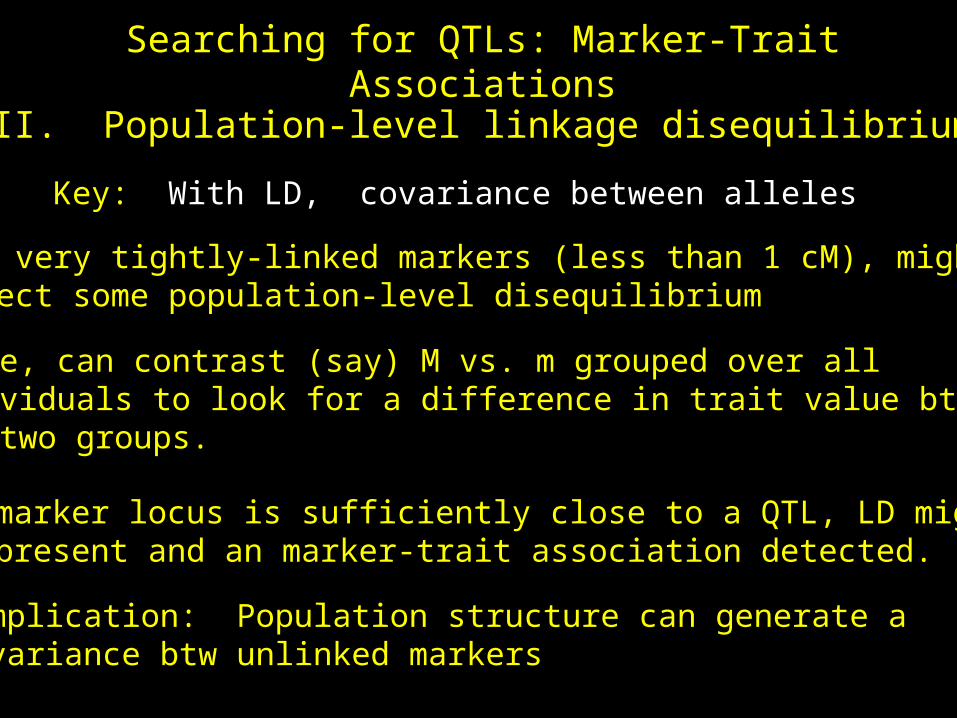
Searching for QTLs: Marker-Trait Associations

II. Population-level linkage disequilibrium

Key: With LD, covariance between alleles

For very tightly-linked markers (less than 1 cM), mightexpect some population-level disequilibrium

Hence, can contrast (say) M vs. m grouped over allindividuals to look for a difference in trait value btwthe two groups.

If marker locus is sufficiently close to a QTL, LD mightbe present and an marker-trait association detected.

Complication: Population structure can generate acovariance btw unlinked markers

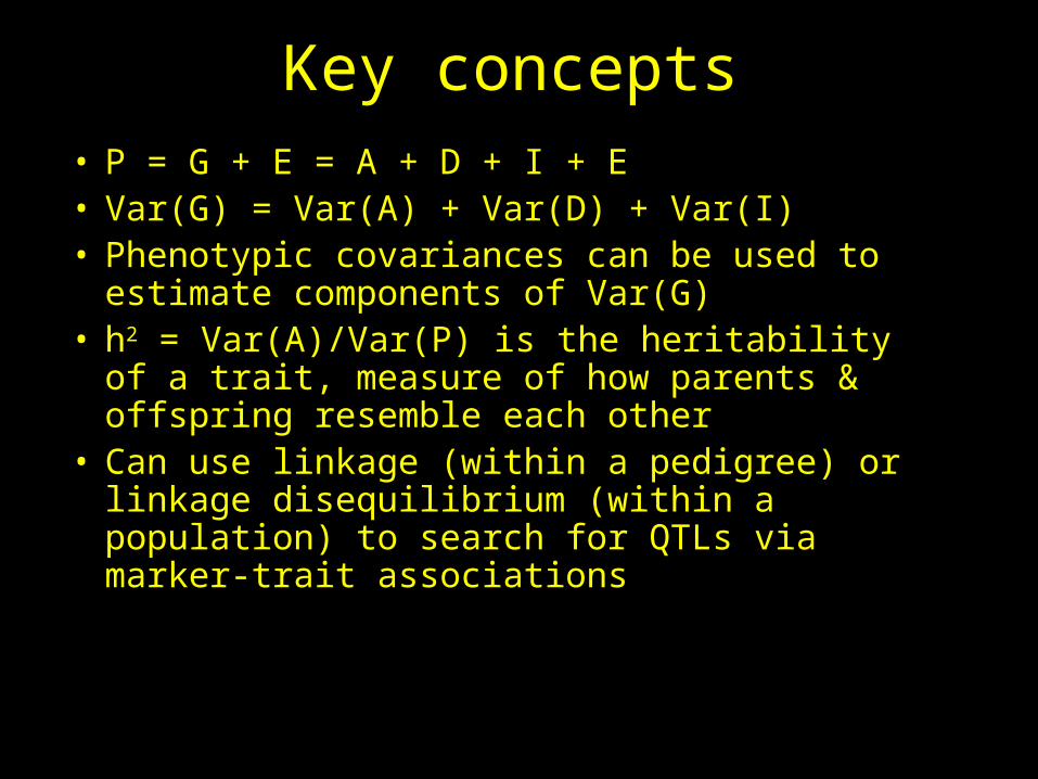
Key concepts• P = G + E = A + D + I + E• Var(G) = Var(A) + Var(D) + Var(I)• Phenotypic covariances can be used to

estimate components of Var(G)• h2 = Var(A)/Var(P) is the heritability of a

trait, measure of how parents & offspring resemble each other

• Can use linkage (within a pedigree) or linkage disequilibrium (within a population) to search for QTLs via marker-trait associations