1

Introduction to Fluid Dynamics

Roger K. Smith

Skript - auf englisch!

Umsonst im Internethttp://www .meteo.physik.uni-muenchen.de

Wählen:LehreManuskripteDownload

User Name: meteo Password: download

2

To provide a survey of basic concepts in fluiddynamics as a preliminary to the study ofdynamical meteorology.

Based on a more extensive course of lectures prepared by Professor B. R. Morton of Monash University, Australia.

A useful reference is: D. J. Acheson

Aim

Description of fluid flow

u u= ( , )x t

In general, this will define a vector field of position and time.

Steady flow occurs when u is independent of time - i.e.

Otherwise the flow is unsteady.

∂ ∂u / t ≡ 0

The description of a fluid flow requires a specification ordetermination of the velocity field, i.e. a specification of the fluid velocity at every point in the region.

3

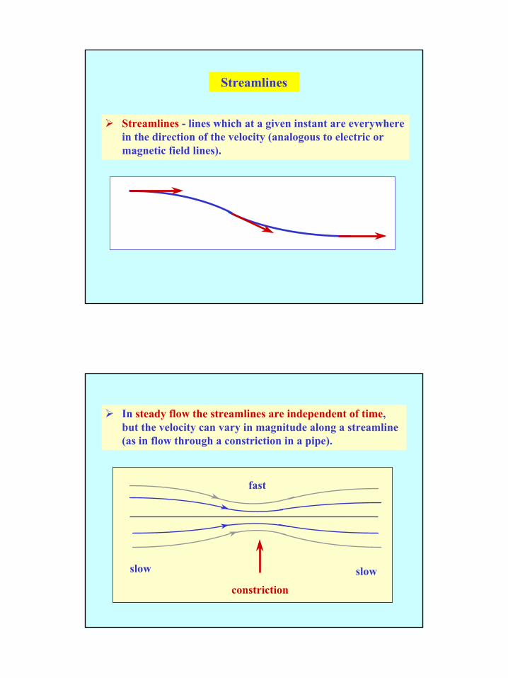
Streamlines - lines which at a given instant are everywhere in the direction of the velocity (analogous to electric or magnetic field lines).

Streamlines

fast

slowslow

constriction

In steady flow the streamlines are independent of time, but the velocity can vary in magnitude along a streamline (as in flow through a constriction in a pipe).

4

Streamlines

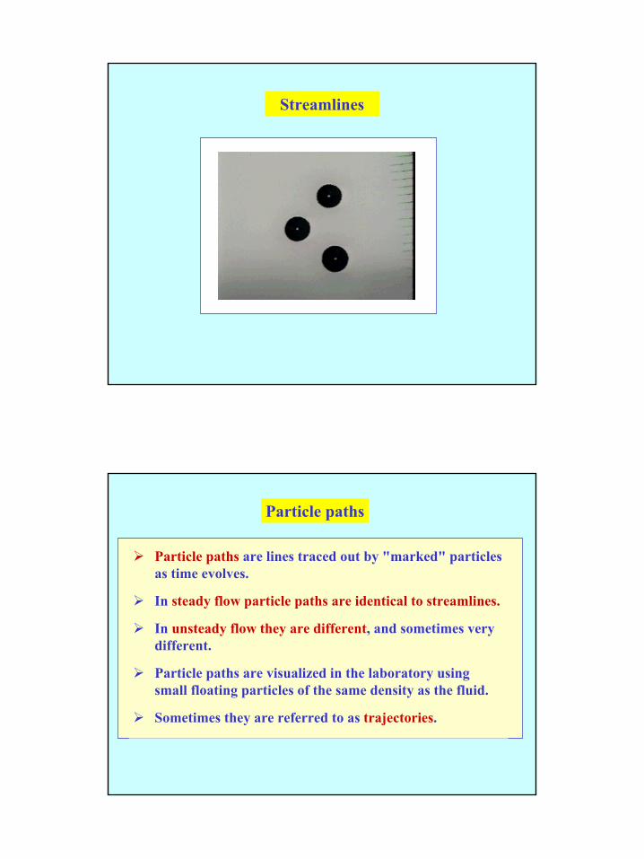
Particle paths are lines traced out by "marked" particles as time evolves.

In steady flow particle paths are identical to streamlines.

In unsteady flow they are different, and sometimes very different.

Particle paths are visualized in the laboratory using small floating particles of the same density as the fluid.

Sometimes they are referred to as trajectories.

Particle paths

5

Filament lines or streaklines are traced out over time by all particles passing through a given point.

They may be visualized, for example, using a hypodermic needle and releasing a slow stream of dye.

In steady flow these are streamlines.

In unsteady flow they are neither streamlines nor particle paths.

Filament lines or streaklines

Streaklines

6

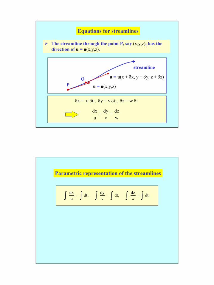
Equations for streamlines

u = u(x,y,z)PQ

streamline

u = u(x + δx, y + δy, z + δz)

δx = u δt , δy = v δt , δz = w δt

dxu

dyv

dzw

= =

The streamline through the point P, say (x,y,z), has the direction of u = u(x,y,z).

dx dy dzdt, dt, dtu v w

= = =∫ ∫ ∫ ∫ ∫ ∫

Parametric representation of the streamlines

7

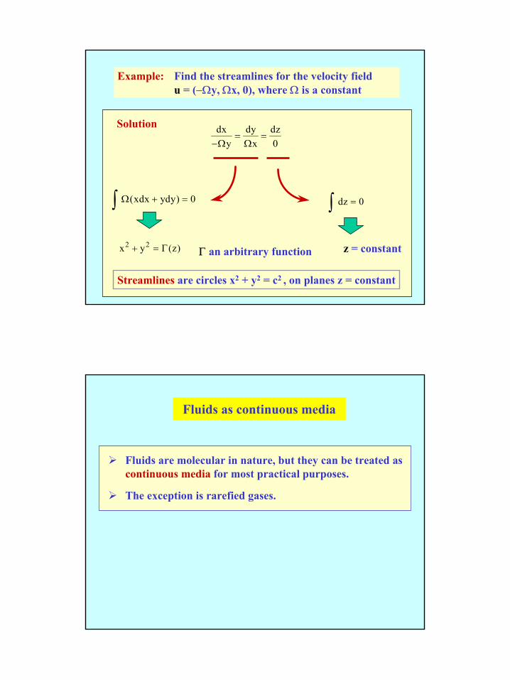
Example: Find the streamlines for the velocity fieldu = (−Ωy, Ωx, 0), where Ω is a constant

Solution dxy

dyx

dz−

= =Ω Ω 0

(xdx ydy) 0Ω + =∫ dz 0=∫

x y z2 2+ = Γ( ) Γ an arbitrary function z = constant

Streamlines are circles x2 + y2 = c2 , on planes z = constant

Fluids are molecular in nature, but they can be treated ascontinuous media for most practical purposes.

The exception is rarefied gases.

Fluids as continuous media

8

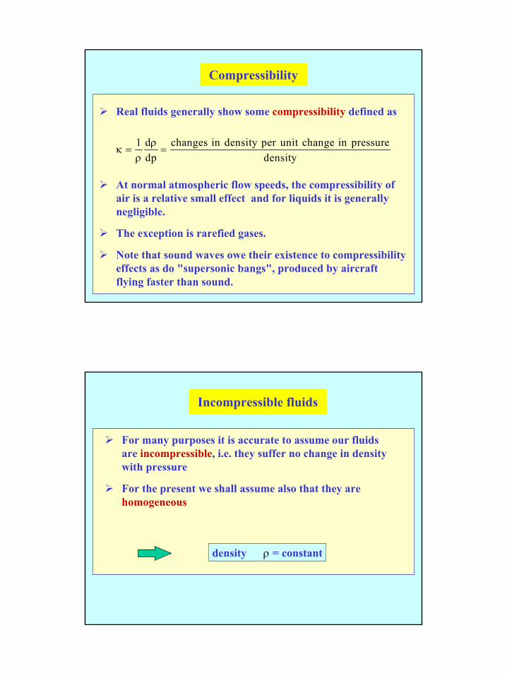
κρ

ρ= =

1 ddp

changes in density per unit change in pressuredensity

At normal atmospheric flow speeds, the compressibility of air is a relative small effect and for liquids it is generally negligible.

The exception is rarefied gases.

Note that sound waves owe their existence to compressibility effects as do "supersonic bangs", produced by aircraft flying faster than sound.

Real fluids generally show some compressibility defined as

Compressibility

density ρ = constant

For many purposes it is accurate to assume our fluids are incompressible, i.e. they suffer no change in density with pressure

For the present we shall assume also that they are homogeneous

Incompressible fluids

9

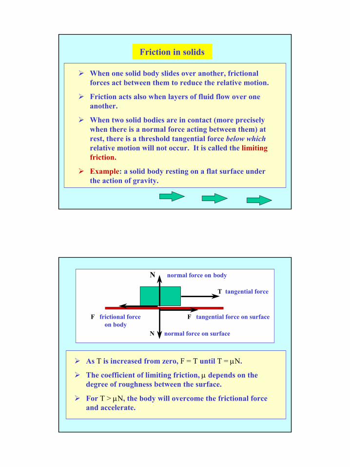
When one solid body slides over another, frictional forces act between them to reduce the relative motion.

Friction acts also when layers of fluid flow over one another.

When two solid bodies are in contact (more precisely when there is a normal force acting between them) at rest, there is a threshold tangential force below whichrelative motion will not occur. It is called the limiting friction.

Example: a solid body resting on a flat surface under the action of gravity.

Friction in solids

N normal force on body

N normal force on surface

F tangential force on surface

T tangential force

F frictional force on body

As T is increased from zero, F = T until T = µN.

The coefficient of limiting friction, µ depends on the degree of roughness between the surface.

For T > µN, the body will overcome the frictional force and accelerate.

10

A distinguishing characteristic of most fluids in their inability to support tangential stresses between layers without motion occurring; i.e. there is no analogue of limiting friction.

Exception: certain types of so-called visco-elastic fluids e.g. paint.

Fluids compared with solids

A visco-elastic fluid

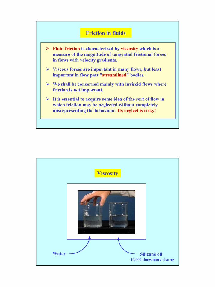
A mixture of water and corn starch, when placed on a flat surface, flows as a thick, viscous fluid. However, when the mixture is rapidly disturbed, it appears to fracture and behave more like a solid.

11

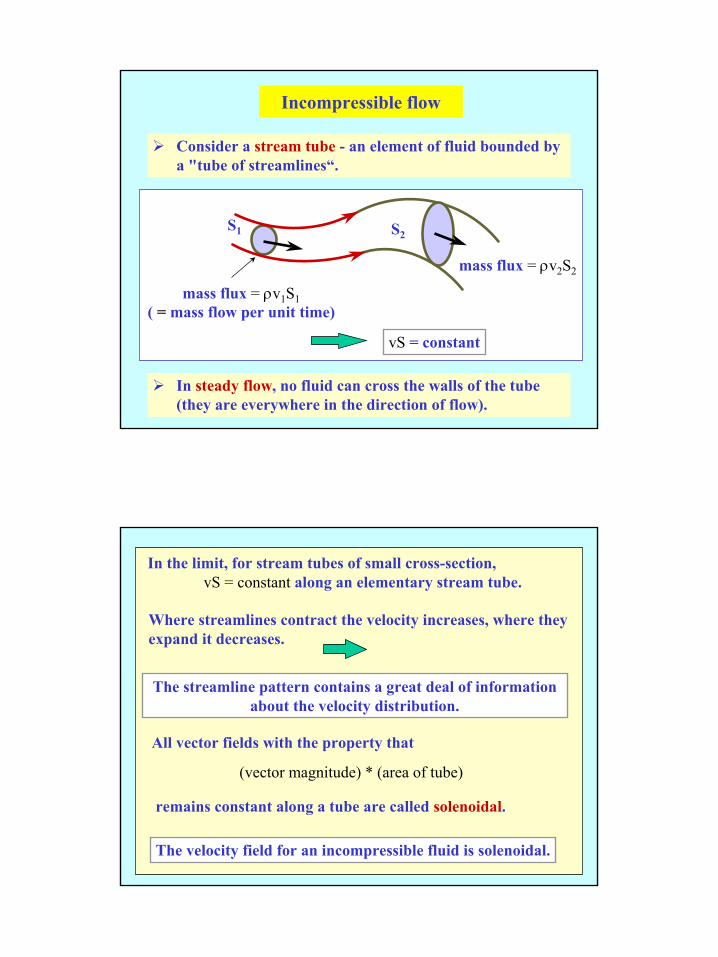
Fluid friction is characterized by viscosity which is a measure of the magnitude of tangential frictional forces in flows with velocity gradients.

Viscous forces are important in many flows, but least important in flow past "streamlined" bodies.

We shall be concerned mainly with inviscid flows where friction is not important.

It is essential to acquire some idea of the sort of flow in which friction may be neglected without completely misrepresenting the behaviour. Its neglect is risky!

Friction in fluids

Water Silicone oil10,000 times more viscous

Viscosity

12

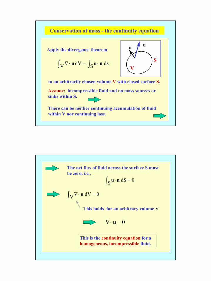
S1 S2

mass flux = ρv1S1( = mass flow per unit time)

mass flux = ρv2S2

vS = constant

Consider a stream tube - an element of fluid bounded by a "tube of streamlines“.

In steady flow, no fluid can cross the walls of the tube (they are everywhere in the direction of flow).

Incompressible flow

In the limit, for stream tubes of small cross-section,vS = constant along an elementary stream tube.

Where streamlines contract the velocity increases, where they expand it decreases.

All vector fields with the property that

(vector magnitude) * (area of tube)

remains constant along a tube are called solenoidal.

The streamline pattern contains a great deal of information about the velocity distribution.

The velocity field for an incompressible fluid is solenoidal.

13

Apply the divergence theorem

dV dsV S∇ ⋅ = ⋅∫ ∫u u nV

S

n u

to an arbitrarily chosen volume V with closed surface S.

Assume: incompressible fluid and no mass sources or sinks within S.

There can be neither continuing accumulation of fluid within V nor continuing loss.

Conservation of mass - the continuity equation

dS 0S ⋅ =∫ u n

This holds for an arbitrary volume V

∇⋅ =u 0

This is the continuity equation for a homogeneous, incompressible fluid.

dV 0V∇ ⋅ =∫ u

The net flux of fluid across the surface S must be zero, i.e.,

14

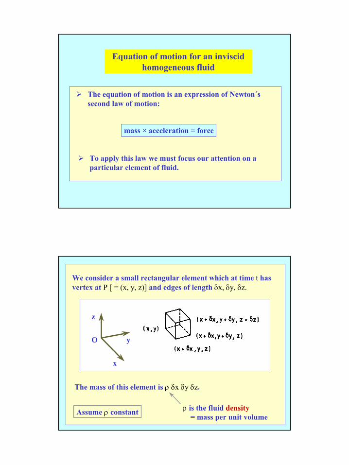
Equation of motion for an inviscid homogeneous fluid

mass × acceleration = force

The equation of motion is an expression of Newton´s second law of motion:

To apply this law we must focus our attention on a particular element of fluid.

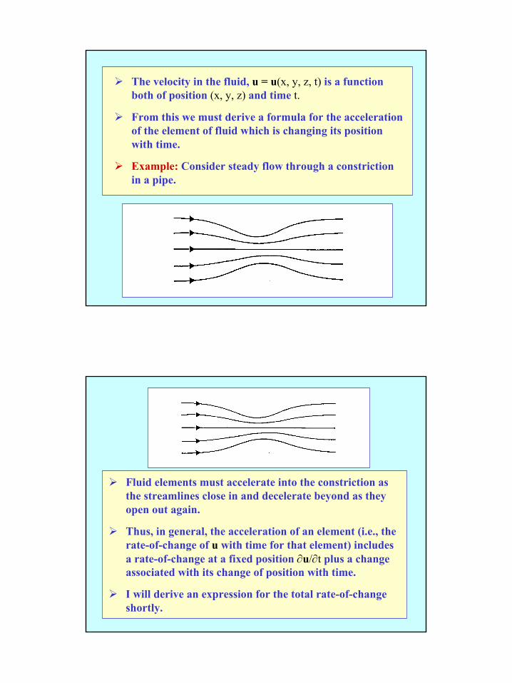
We consider a small rectangular element which at time t has vertex at P [ = (x, y, z)] and edges of length δx, δy, δz.

The mass of this element is ρ δx δy δz.

Assume ρ constant

z

O

x

y

ρ is the fluid density= mass per unit volume

15

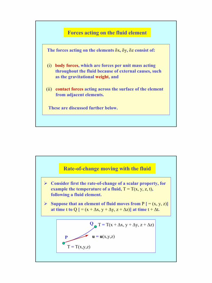
The velocity in the fluid, u = u(x, y, z, t) is a function both of position (x, y, z) and time t.

From this we must derive a formula for the acceleration of the element of fluid which is changing its position with time.

Example: Consider steady flow through a constriction in a pipe.

Fluid elements must accelerate into the constriction as the streamlines close in and decelerate beyond as they open out again.

Thus, in general, the acceleration of an element (i.e., the rate-of-change of u with time for that element) includes a rate-of-change at a fixed position ∂u/∂t plus a change associated with its change of position with time.

I will derive an expression for the total rate-of-change shortly.

16

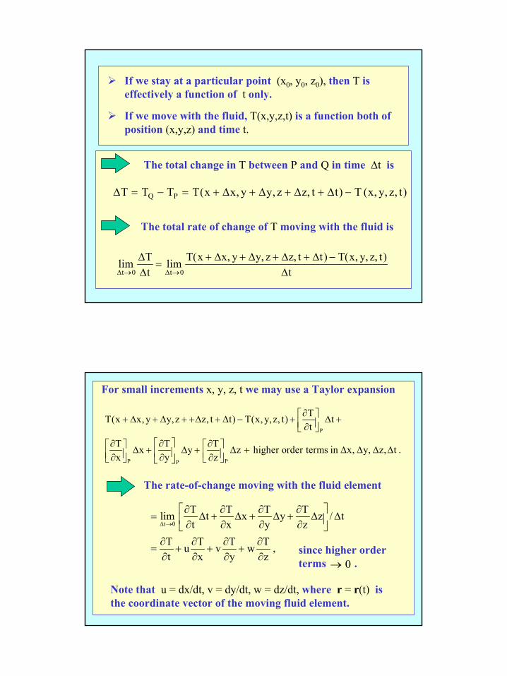
The forces acting on the elements δx, δy, δz consist of:

(i) body forces, which are forces per unit mass actingthroughout the fluid because of external causes, suchas the gravitational weight, and

(ii) contact forces acting across the surface of the element from adjacent elements.

These are discussed further below.

Forces acting on the fluid element

T = T(x,y,z)

P

Q T = T(x + ∆x, y + ∆y, z + ∆z)

u = u(x,y,z)

Consider first the rate-of-change of a scalar property, for example the temperature of a fluid, T = T(x, y, z, t), following a fluid element.

Suppose that an element of fluid moves from P [ = (x, y, z)] at time t to Q [ = (x + ∆x, y + ∆y, z + ∆z)] at time t + ∆t.

Rate-of-change moving with the fluid

17

The total change in T between P and Q in time ∆t is

∆ ∆ ∆ ∆ ∆T T T T x x y y z z t t T x y z tQ P= − = + + + + −( , , , ) ( , , , )

The total rate of change of T moving with the fluid is

lim lim ( , , , ) ( , , , )∆ ∆

∆∆

∆ ∆ ∆ ∆∆t t

Tt

T x x y y z z t t T x y z tt→ →

=+ + + + −

0 0

If we stay at a particular point (x0, y0, z0), then T is effectively a function of t only.

If we move with the fluid, T(x,y,z,t) is a function both of position (x,y,z) and time t.

For small increments x, y, z, t we may use a Taylor expansion

P

P PP

TT(x x, y y,z z, t t) T(x, y,z, t) tt

T T Tx y z higher order terms in x, y, z, t .x y z

∂ + ∆ + ∆ + +∆ + ∆ − + ∆ + ∂

∂ ∂ ∂ ∆ + ∆ + ∆ + ∆ ∆ ∆ ∆ ∂ ∂ ∂

The rate-of-change moving with the fluid element

t 0

T T T Tlim t x y z / tt x y z

T T T Tu v w ,t x y z

∆ →

∂ ∂ ∂ ∂= ∆ + ∆ + ∆ + ∆ ∆ ∂ ∂ ∂ ∂ ∂ ∂ ∂ ∂

= + + +∂ ∂ ∂ ∂ since higher order

terms .→ 0

Note that u = dx/dt, v = dy/dt, w = dz/dt, where r = r(t) is the coordinate vector of the moving fluid element.

18

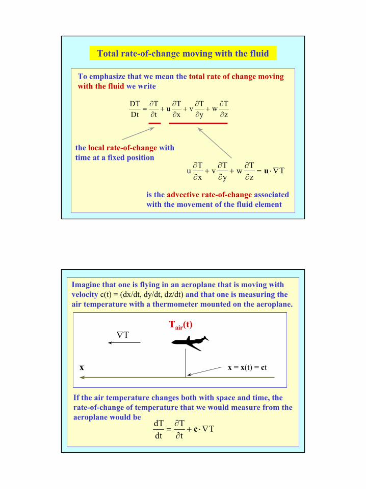
To emphasize that we mean the total rate of change moving with the fluid we write

DTDt

Tt

u Tx

v Ty

w Tz

= + + +∂∂

∂∂

∂∂

∂∂

the local rate-of-change with time at a fixed position

u Tx

v Ty

w Tz

T∂∂

∂∂

∂∂

+ + = ⋅∇u

is the advective rate-of-change associated with the movement of the fluid element

Total rate-of-change moving with the fluid

Imagine that one is flying in an aeroplane that is moving with velocity c(t) = (dx/dt, dy/dt, dz/dt) and that one is measuring the air temperature with a thermometer mounted on the aeroplane.

x x = x(t) = ct

If the air temperature changes both with space and time, the rate-of-change of temperature that we would measure from the aeroplane would be

∇TTair(t)

dTdt

Tt

T= + ⋅∇∂∂

c

19

dTdt

Tt

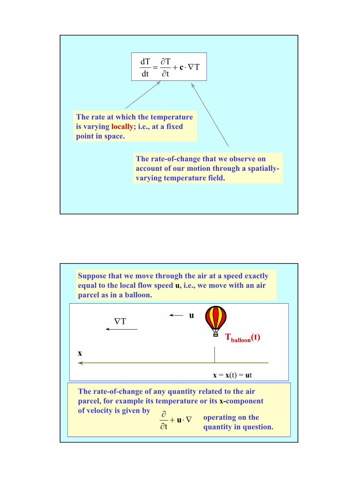
T= + ⋅∇∂∂

c

The rate at which the temperature is varying locally; i.e., at a fixed point in space.

The rate-of-change that we observe on account of our motion through a spatially-varying temperature field.

Suppose that we move through the air at a speed exactly equal to the local flow speed u, i.e., we move with an air parcel as in a balloon.

∂∂t+ ⋅∇u

The rate-of-change of any quantity related to the air parcel, for example its temperature or its x-component of velocity is given by

∇T

x

x = x(t) = ut

u

Tballoon(t)

operating on the quantity in question.

20

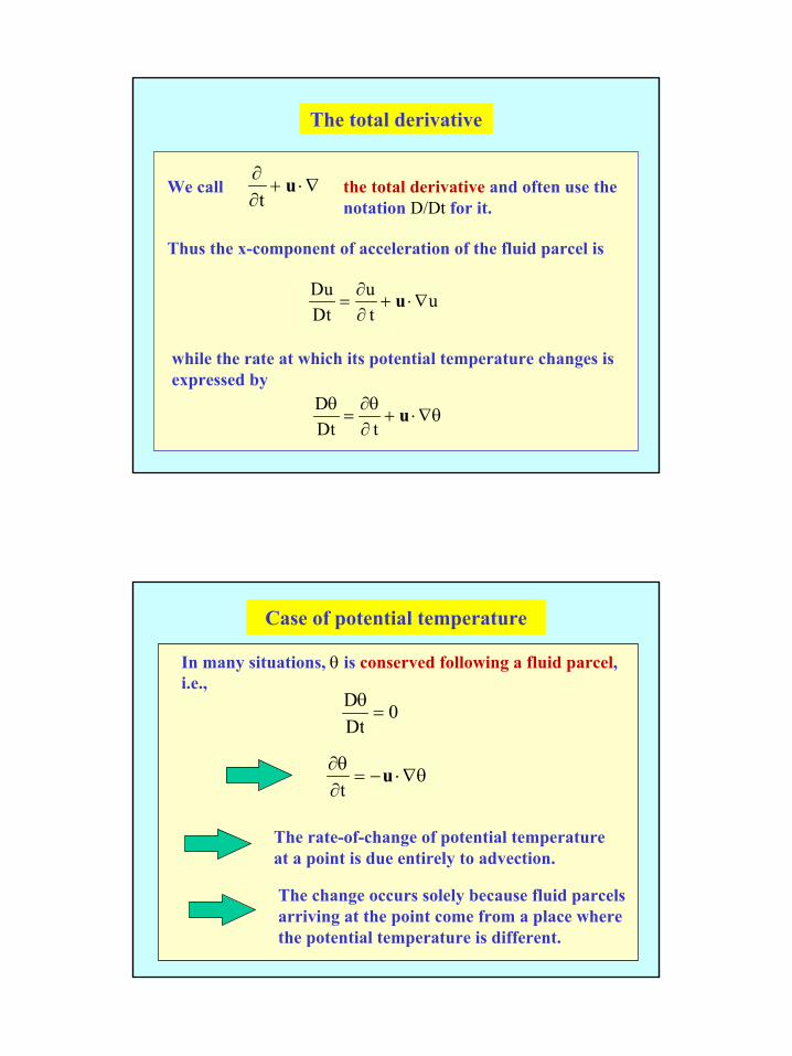
the total derivative and often use the notation D/Dt for it.

DuDt

ut

u= + ⋅∇∂∂

u

while the rate at which its potential temperature changes is expressed by

DDt tθ ∂θ

∂= + ⋅∇θu

∂∂t+ ⋅∇uWe call

Thus the x-component of acceleration of the fluid parcel is

The total derivative

In many situations, θ is conserved following a fluid parcel, i.e.,

0DtD

=θ

∂θ∂t

= − ⋅∇θu

The rate-of-change of potential temperature at a point is due entirely to advection.

The change occurs solely because fluid parcels arriving at the point come from a place where the potential temperature is different.

Case of potential temperature

21

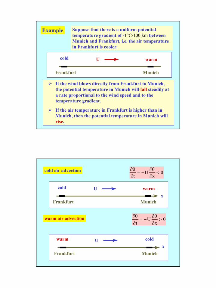
Suppose that there is a uniform potential temperature gradient of -1°C/100 km between Munich and Frankfurt, i.e. the air temperature in Frankfurt is cooler.

Example

Frankfurt Munich

Ucold warm

If the wind blows directly from Frankfurt to Munich, the potential temperature in Munich will fall steadily at a rate proportional to the wind speed and to the temperature gradient.

If the air temperature in Frankfurt is higher than in Munich, then the potential temperature in Munich will rise.

Frankfurt Munich

Ucold warm

Frankfurt Munich

U coldwarm

x

x

cold air advection

warm air advection

∂θ∂

∂θ∂t

Ux

= − < 0

∂θ∂

∂θ∂t

Ux

= − > 0

22

Example

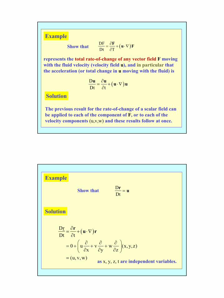
Show that ( )DFDt T

∂= + ⋅∇∂

F u F

represents the total rate-of-change of any vector field F moving with the fluid velocity (velocity field u), and in particular that the acceleration (or total change in u moving with the fluid) is

( )DDt t

∂= + ⋅∇∂

u u u u

The previous result for the rate-of-change of a scalar field can be applied to each of the component of F, or to each of the velocity components (u,v,w) and these results follow at once.

Solution

Show that DDt

r u=

Solution

( )DrDt t

0 u v w (x, y,z)x y z

(u, v, w)

∂= + ⋅∇∂

∂ ∂ ∂= + + + ∂ ∂ ∂ =

r u r

Example

as x, y, z, t are independent variables.

23

Are the two x-components in rectangular Cartesian coordinates,

( )x⋅∇u u and ( )21

2 x∇ u

the same or different?

( ) ( )212⋅∇ = ∇ − ∧u u u u ω

Question

Note that