Introduction to Finite Element Analysis using ANSYS to Finite Element Analysis using ANSYS Sasi Kumar Tippabhotla PhD Candidate Xtreme Photovoltaics (XPV) Lab EPD, SUTD Disclaimer:

Introduction to Finite Element Analysis using ANSYS

Sasi Kumar Tippabhotla

PhD Candidate

Xtreme Photovoltaics (XPV) Lab

EPD, SUTD

Disclaimer: The material and simulations (using Ansys student version) presented in this document are made purely for teaching and sharing knowledge and NOT made for commercial use. The concepts and examples (other than author’s own research) presented here were taken from publicly available references or internet. In both the cases, the original references / sources were properly acknowledged. This document is expected to be used only for personal learning / teaching purpose.

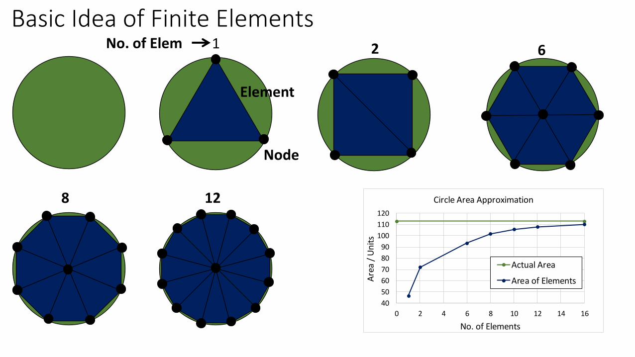
Basic Idea of Finite Elements

Element

Node

1 2 6

8 12

40

50

60

70

80

90

100

110

120

0 2 4 6 8 10 12 14 16

Are

a /

Un

its

No. of Elements

Circle Area Approximation

Actual Area

Area of Elements

No. of Elem

Finite Element Method

• A numerical method to solve (partial) differential equations• Gives only approximate solution• Applicable to several physical domains, for ex.

• Structural• Thermal / Fluid• Electromagnetic• Coupled field

• Discretization of the structure into small portions – Elements• Connecting points between elements – Nodes

Finite Element Analysis Procedure (Structures)

• Pre-processing• Discretization of the structure – Meshing• Assign element type and properties• Assign material properties• Apply Boundary conditions and Loads

• Solution• Select the solver• Calculate element stiffness matrices• Assemble global stiffness matrix• Solve for displacements, strains, stresses etc.

• Post-processing• Display / Output displacements, strains, stresses etc.• Calculate user defined parameters from the results

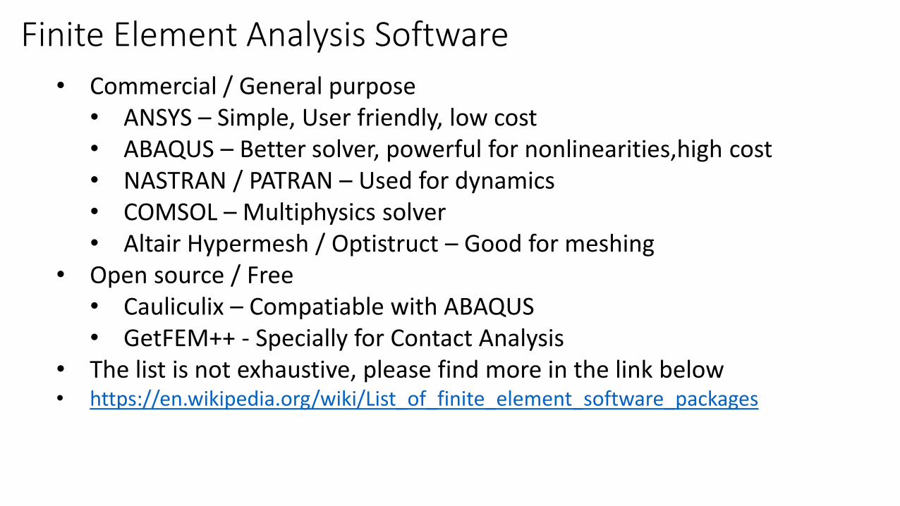
Finite Element Analysis Software

• Commercial / General purpose• ANSYS – Simple, User friendly, low cost• ABAQUS – Better solver, powerful for nonlinearities,high cost • NASTRAN / PATRAN – Used for dynamics• COMSOL – Multiphysics solver• Altair Hypermesh / Optistruct – Good for meshing

• Open source / Free• Cauliculix – Compatiable with ABAQUS• GetFEM++ - Specially for Contact Analysis

• The list is not exhaustive, please find more in the link below• https://en.wikipedia.org/wiki/List_of_finite_element_software_packages

https://en.wikipedia.org/wiki/List_of_finite_element_software_packages

Finite Element Analysis - Uses

• New Product Design• Virtual Design of Experiments (DoE)• Fatigue Life / Fracture estimation• Design Optimization • Identification of sensor locations for testing

/ validation• Sensitivity analysis

• Existing Product• Feasibility of Repairs / Upgrades • Product remaining life estimation• Identification of maintenance intervals• Failure root cause analysis

Reduces new product validation / testing costs

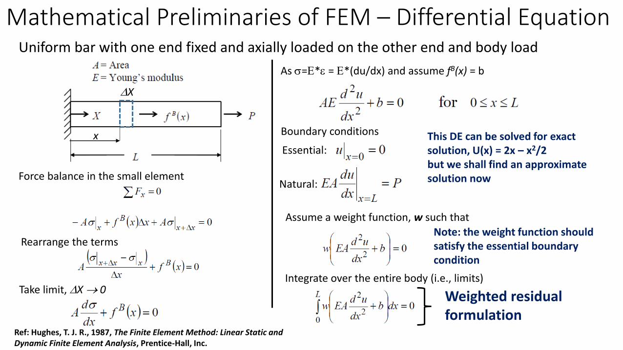
Mathematical Preliminaries of FEM – Differential Equation

X

x

Rearrange the terms

Take limit, X 0

Uniform bar with one end fixed and axially loaded on the other end and body load

Force balance in the small element

As =* = *(du/dx) and assume fB(x) = b

Boundary conditions This DE can be solved for exact solution, U(x) = 2x – x2/2but we shall find an approximate solution now

Assume a weight function, w such that

Integrate over the entire body (i.e., limits)

Ref: Hughes, T. J. R., 1987, The Finite Element Method: Linear Static and Dynamic Finite Element Analysis, Prentice-Hall, Inc.

Weighted residual formulation

Note: the weight function should satisfy the essential boundary condition

Essential:

Natural:

Mathematical Preliminaries of FEM – Variational Formulation

Advantages:• No second order term – simple to solve numerically• Symmetry• Natural boundary condition is included, need not be

enforced.• No double differentiation requirement for

displacement trail function

Assume an approximate solution, un


Weighted residual formulation

0

Variational Form / Weak Form of the Differential Equation

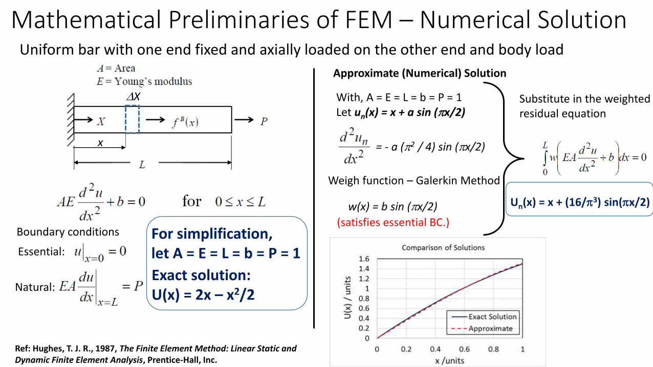
Mathematical Preliminaries of FEM – Numerical Solution

X

x

Uniform bar with one end fixed and axially loaded on the other end and body load


Boundary conditions

Essential:

Natural:Exact solution: U(x) = 2x – x2/2

With, A = E = L = b = P = 1Let un(x) = x + a sin (x/2)

Weigh function – Galerkin Method

= - a (2 / 4) sin (x/2)

w(x) = b sin (x/2) Un(x) = x + (16/3) sin(x/2)

Approximate (Numerical) Solution

(satisfies essential BC.)

Substitute in the weighted residual equation

For simplification, let A = E = L = b = P = 1

Different Types of Elements

1 D (line) Elements

Spring, Truss, Beam, Pipe etc.ni

nj

ek

2 D (Plane) Elements

Plate, Shell, Membrane etc.

ni

nj

nl

nk

ek

3 D (Solid) Elements

3D continuum domains

Special Purpose Elements

Point mass, Contact, Coupling, etc.

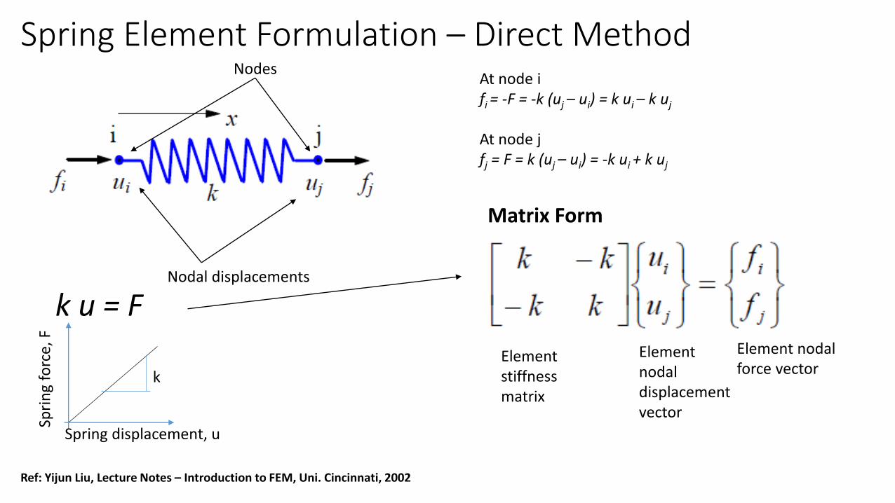
Spring Element Formulation – Direct MethodNodes

Nodal displacements

k u = F

Matrix Form

Elementnodal displacementvector

Element nodal force vector

Element stiffness matrix

Spring displacement, u

Spri

ng

forc

e, F

k

Ref: Yijun Liu, Lecture Notes – Introduction to FEM, Uni. Cincinnati, 2002

At node ifi = -F = -k (uj – ui) = k ui – k uj

At node jfj = F = k (uj – ui) = -k ui + k uj

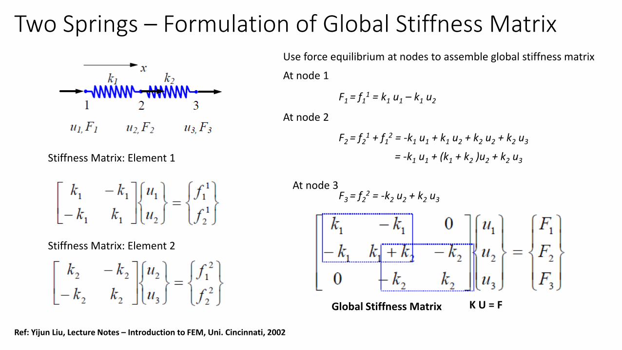
Two Springs – Formulation of Global Stiffness Matrix


Stiffness Matrix: Element 1

Stiffness Matrix: Element 2

Use force equilibrium at nodes to assemble global stiffness matrix

At node 1

F1 = f11 = k1 u1 – k1 u2

At node 2

F2 = f21 + f1

2 = -k1 u1 + k1 u2 + k2 u2 + k2 u3

= -k1 u1 + (k1 + k2 )u2 + k2 u3

Global Stiffness Matrix

F3 = f22 = -k2 u2 + k2 u3

At node 3

K U = F

Elastic Bar Element – FormulationNodal displacements

Nodes

k u = F

Matrix Form

Elementnodal displacementvector

Element nodal force vector

Element stiffness matrix

Displacement, u

Forc

e, F

k = EA/L


At node ifi = -F = -k (uj – ui) = k ui – k uj

At node jfj = F = k (uj – ui) = -k ui + k uj

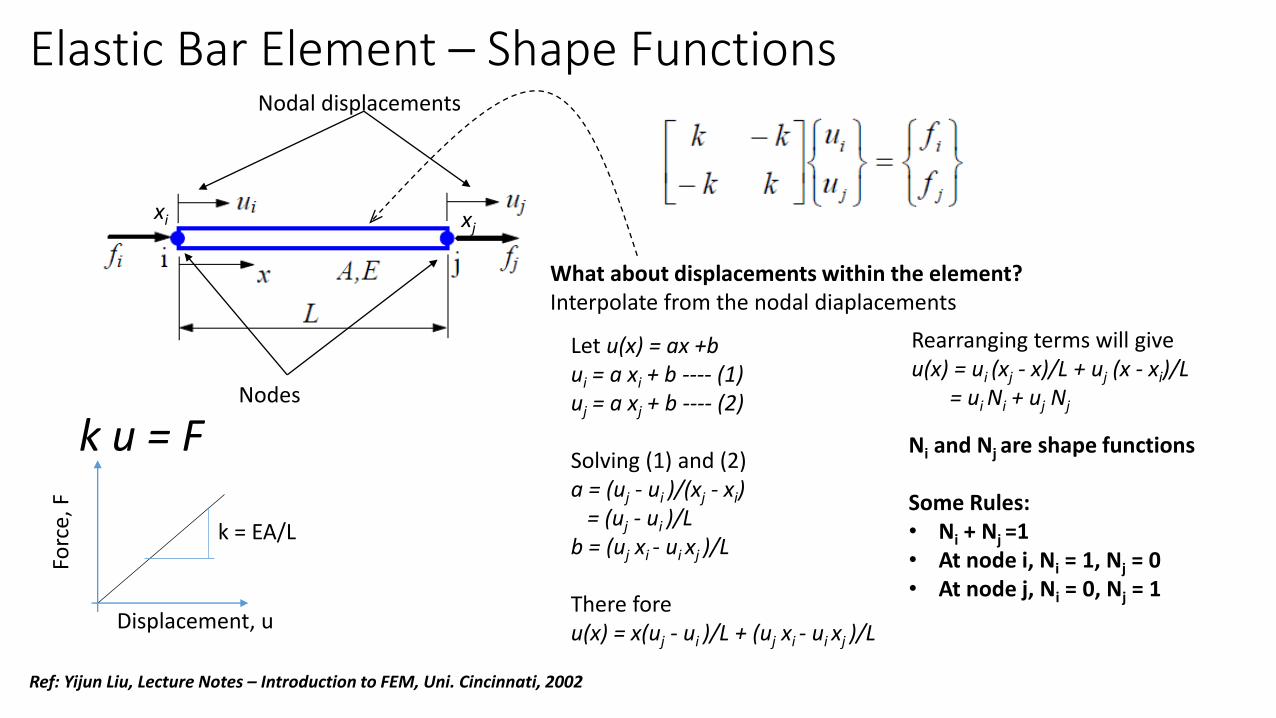
Elastic Bar Element – Shape FunctionsNodal displacements

Nodes

k u = F

Displacement, u

Forc

e, F

k = EA/L


What about displacements within the element?Interpolate from the nodal diaplacements

Let u(x) = ax +bui = a xi + b ---- (1)uj = a xj + b ---- (2)

Solving (1) and (2)a = (uj - ui )/(xj - xi)

= (uj - ui )/Lb = (uj xi - ui xj )/L

There foreu(x) = x(uj - ui )/L + (uj xi - ui xj )/L

xi xj

Rearranging terms will giveu(x) = ui (xj - x)/L + uj (x - xi)/L

= ui Ni + uj Nj

Ni and Nj are shape functions

Some Rules:• Ni + Nj =1• At node i, Ni = 1, Nj = 0• At node j, Ni = 0, Nj = 1

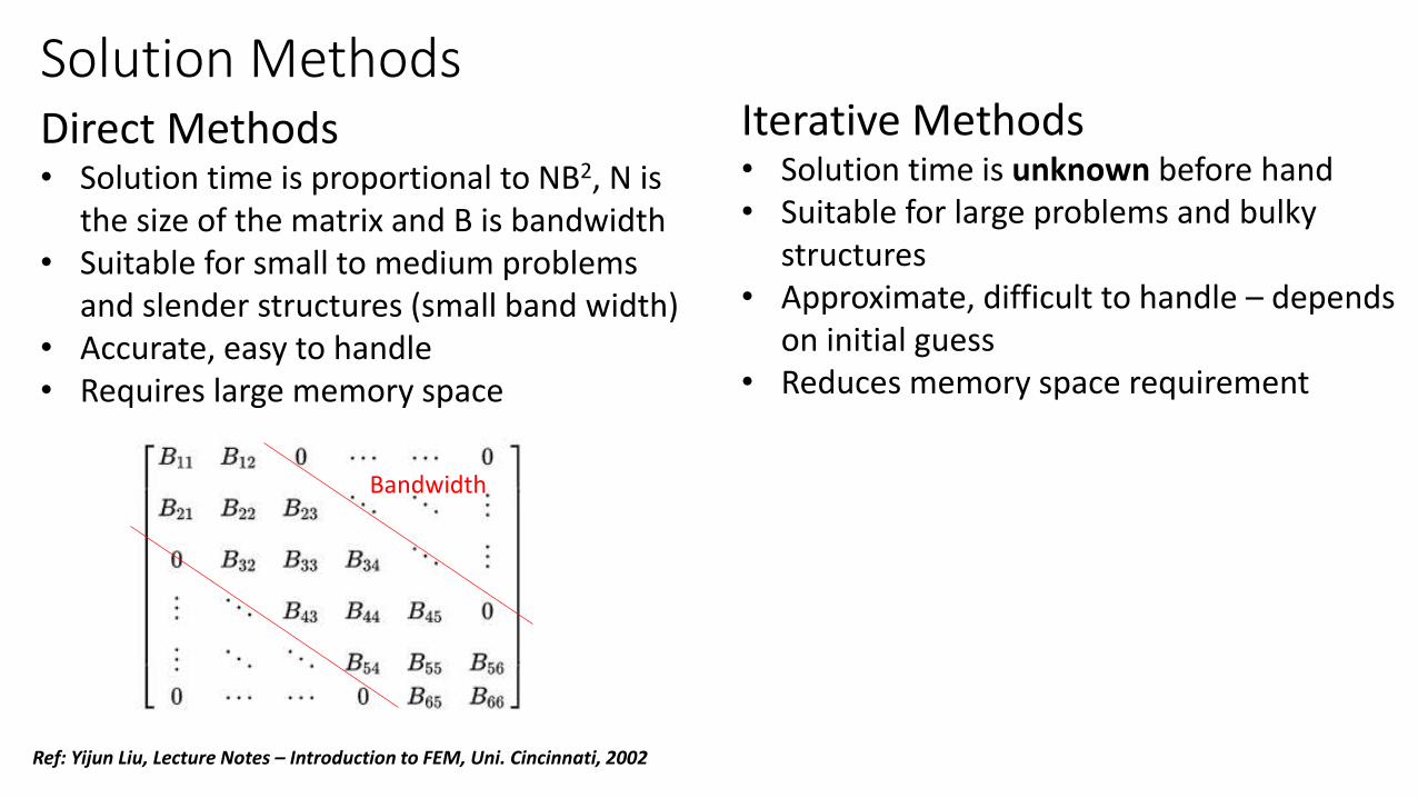
Solution MethodsDirect Methods• Solution time is proportional to NB2, N is

the size of the matrix and B is bandwidth• Suitable for small to medium problems

and slender structures (small band width)• Accurate, easy to handle• Requires large memory space

Iterative Methods• Solution time is unknown before hand• Suitable for large problems and bulky

structures• Approximate, difficult to handle – depends

on initial guess• Reduces memory space requirement


Bandwidth

Solution Methods


Direct Methods – Gauss Elimination Iterative Methods – Gauss-Siedel

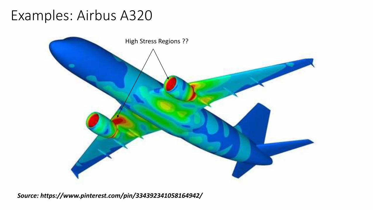
Examples: Airbus A320

Source: https://www.pinterest.com/pin/334392341058164942/

High Stress Regions ??

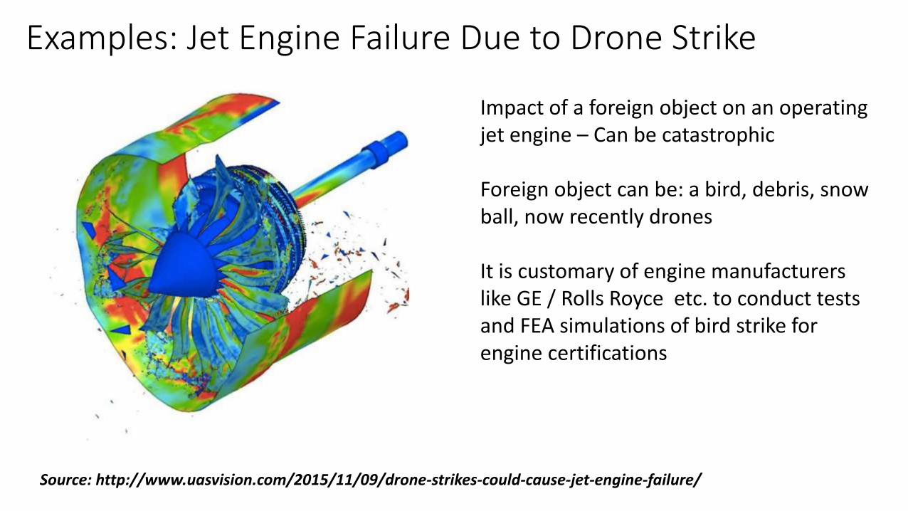
Examples: Jet Engine Failure Due to Drone Strike

Source: http://www.uasvision.com/2015/11/09/drone-strikes-could-cause-jet-engine-failure/

Impact of a foreign object on an operating jet engine – Can be catastrophic

Foreign object can be: a bird, debris, snow ball, now recently drones

It is customary of engine manufacturers like GE / Rolls Royce etc. to conduct tests and FEA simulations of bird strike for engine certifications

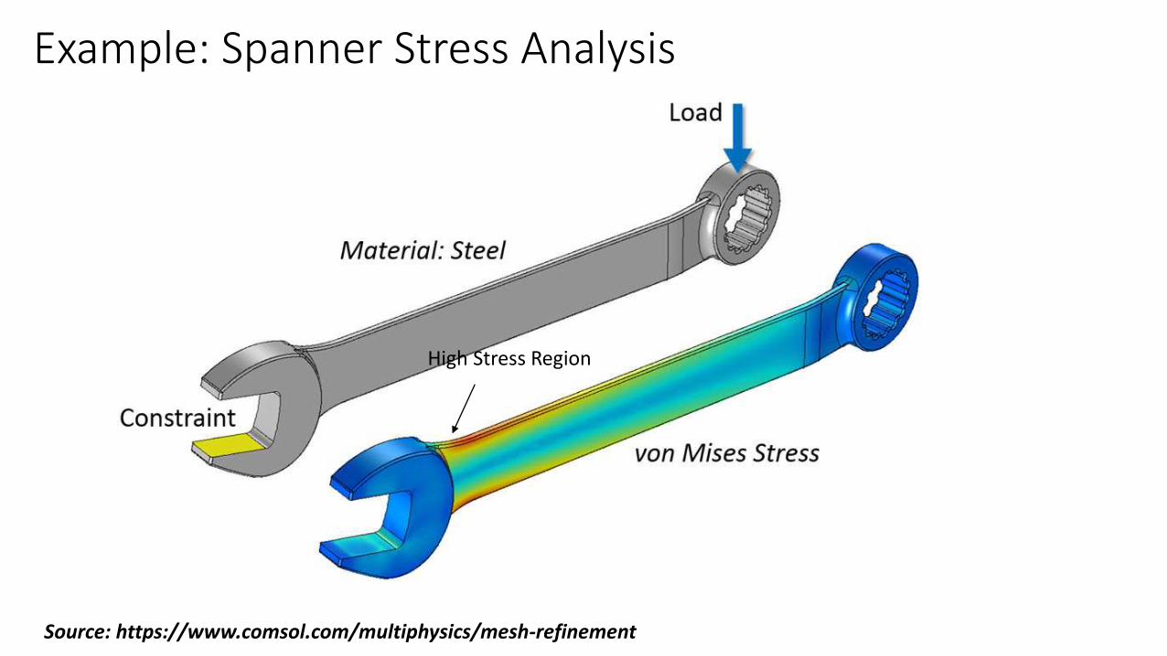
Example: Spanner Stress Analysis

High Stress Region

Source: https://www.comsol.com/multiphysics/mesh-refinement

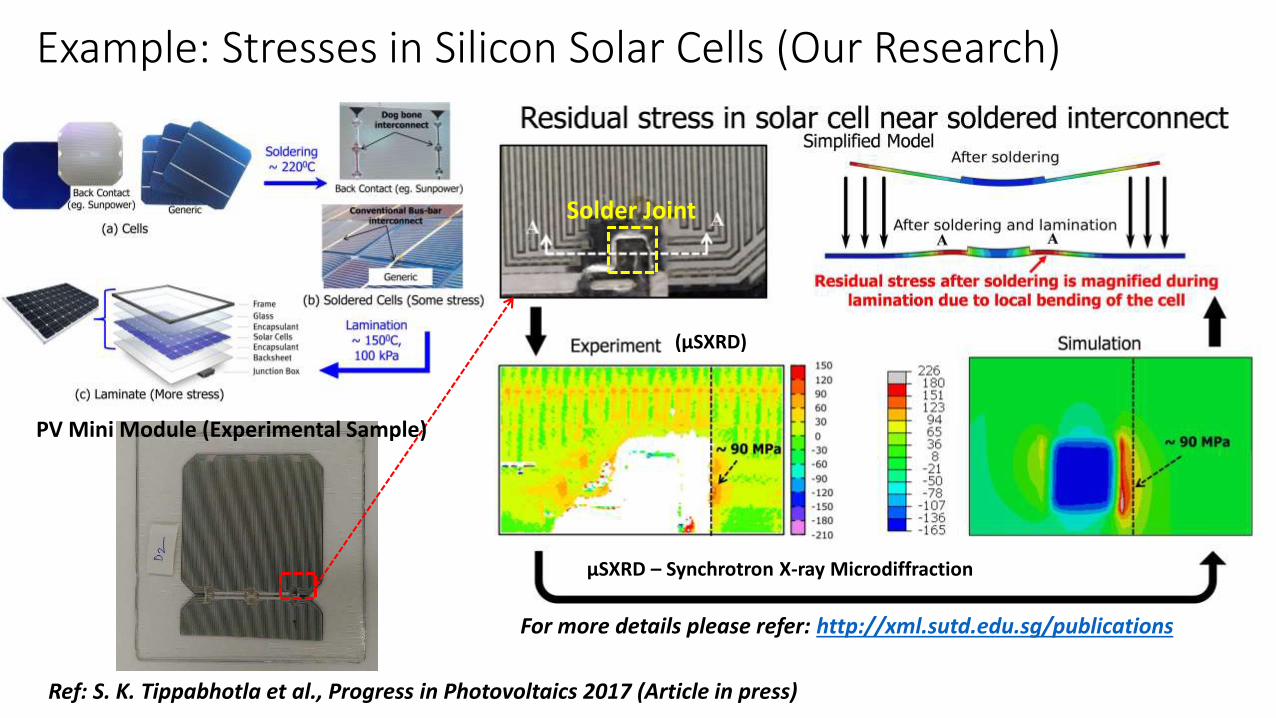
Example: Stresses in Silicon Solar Cells (Our Research)

Ref: S. K. Tippabhotla et al., Progress in Photovoltaics 2017 (Article in press)

Solder Joint

PV Mini Module (Experimental Sample)

(µSXRD)

µSXRD – Synchrotron X-ray Microdiffraction

For more details please refer: http://xml.sutd.edu.sg/publications

http://xml.sutd.edu.sg/publications

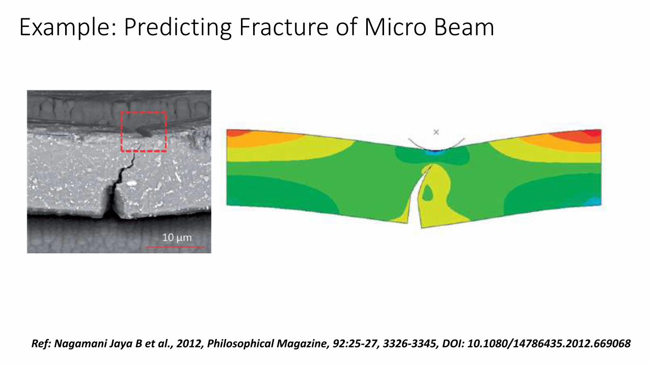
Example: Predicting Fracture of Micro Beam

Ref: Nagamani Jaya B et al., 2012, Philosophical Magazine, 92:25-27, 3326-3345, DOI: 10.1080/14786435.2012.669068

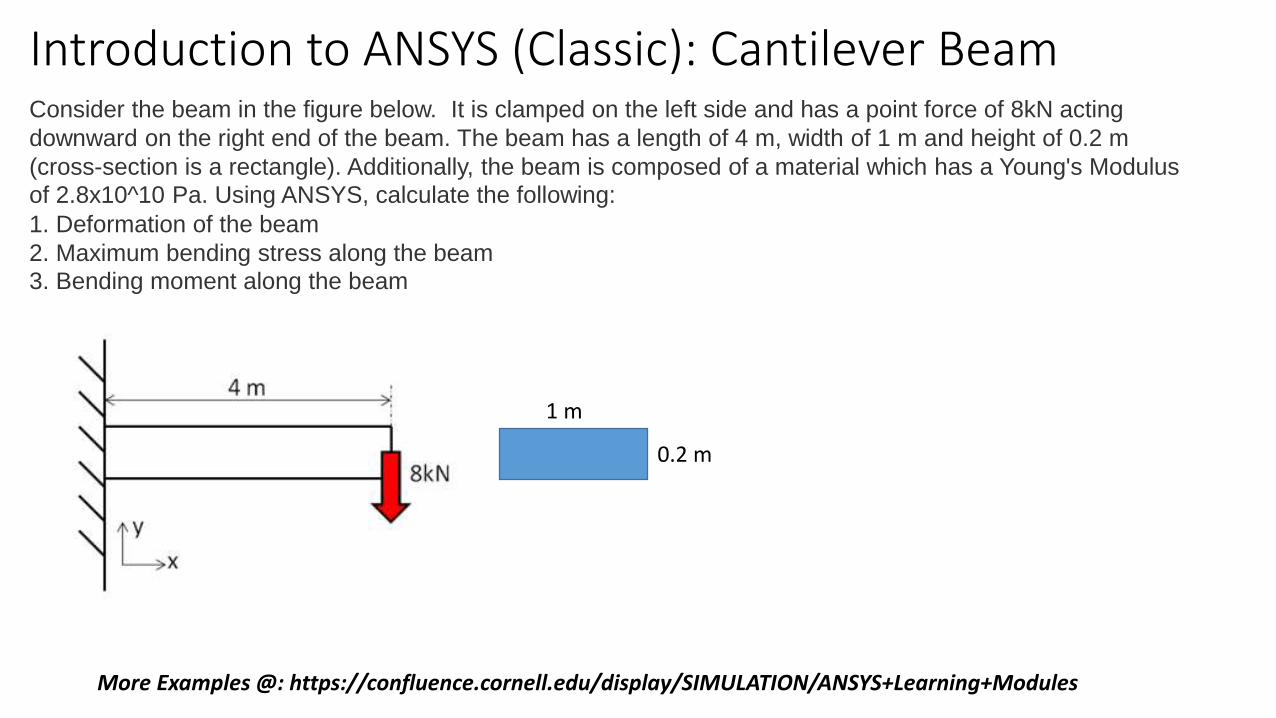
Introduction to ANSYS (Classic): Cantilever Beam

More Examples @: https://confluence.cornell.edu/display/SIMULATION/ANSYS+Learning+Modules

Consider the beam in the figure below. It is clamped on the left side and has a point force of 8kN acting

downward on the right end of the beam. The beam has a length of 4 m, width of 1 m and height of 0.2 m

(cross-section is a rectangle). Additionally, the beam is composed of a material which has a Young's Modulus

of 2.8x10^10 Pa. Using ANSYS, calculate the following:

1. Deformation of the beam

2. Maximum bending stress along the beam

3. Bending moment along the beam

1 m

0.2 m

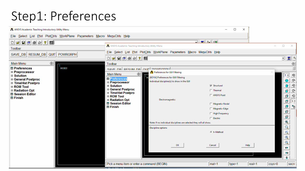
Step1: Preferences

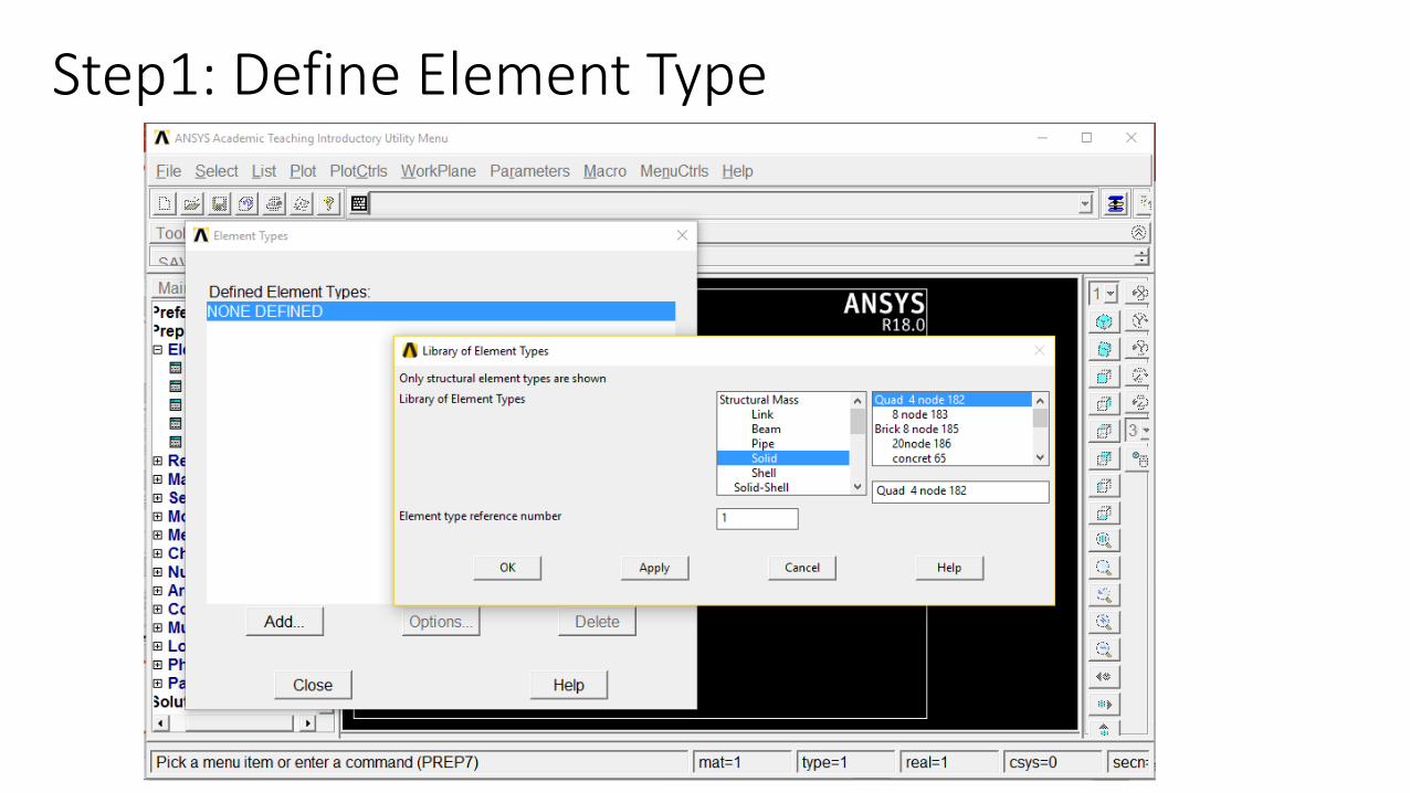
Step1: Define Element Type

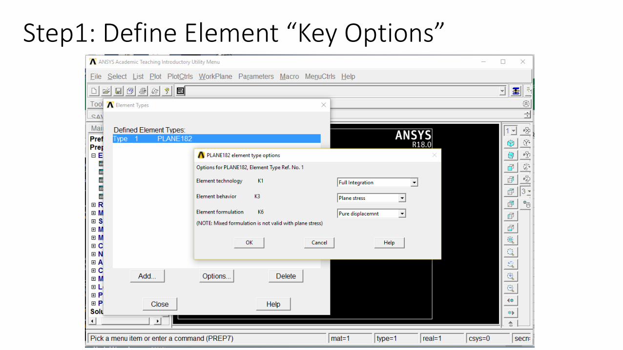
Step1: Define Element “Key Options”

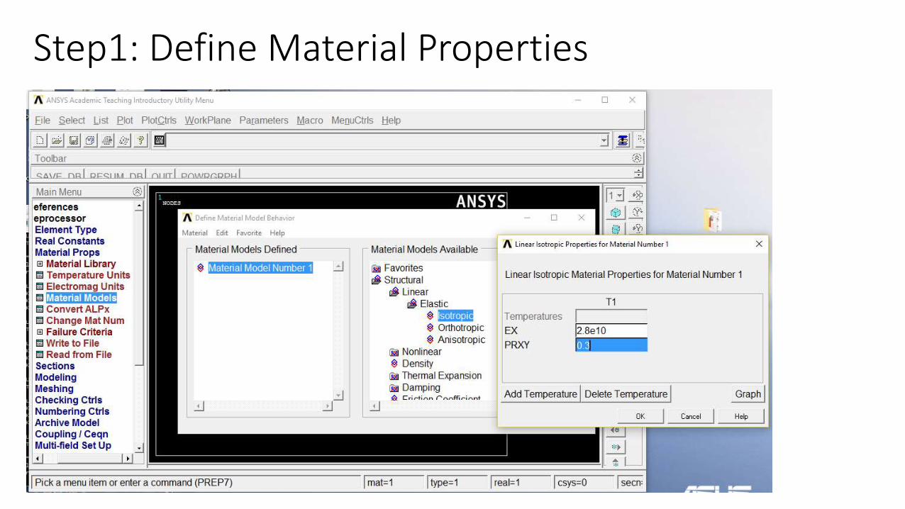
Step1: Define Material Properties

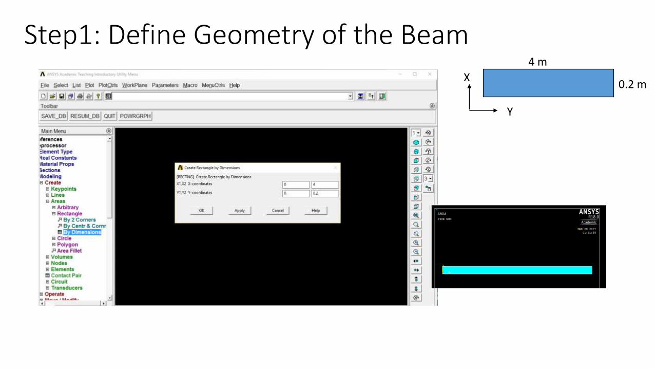
Step1: Define Geometry of the BeamX

Y

4 m

0.2 m

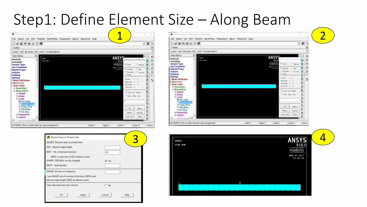
Step1: Define Element Size – Along Beam1 2

3 4

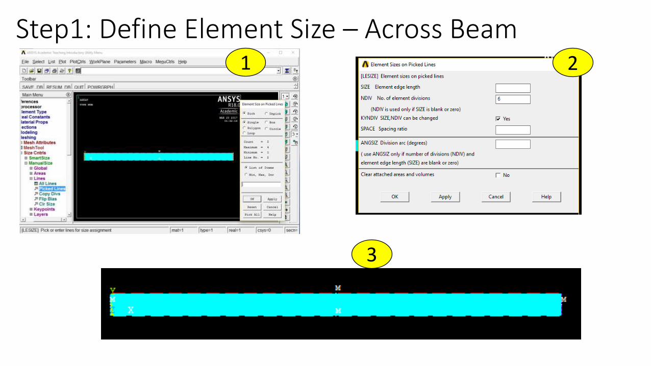
Step1: Define Element Size – Across Beam1 2

3

Step1: Mesh – Mapped mesh by corners

1 2Select the area by clicking on it (notice change of colour?)

Pick corners in cyclic order

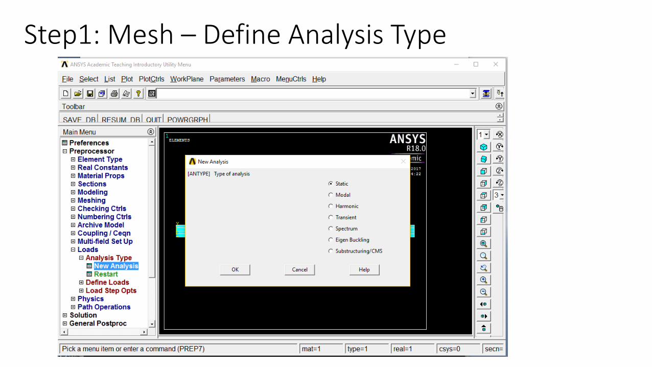
Step1: Mesh – Define Analysis Type

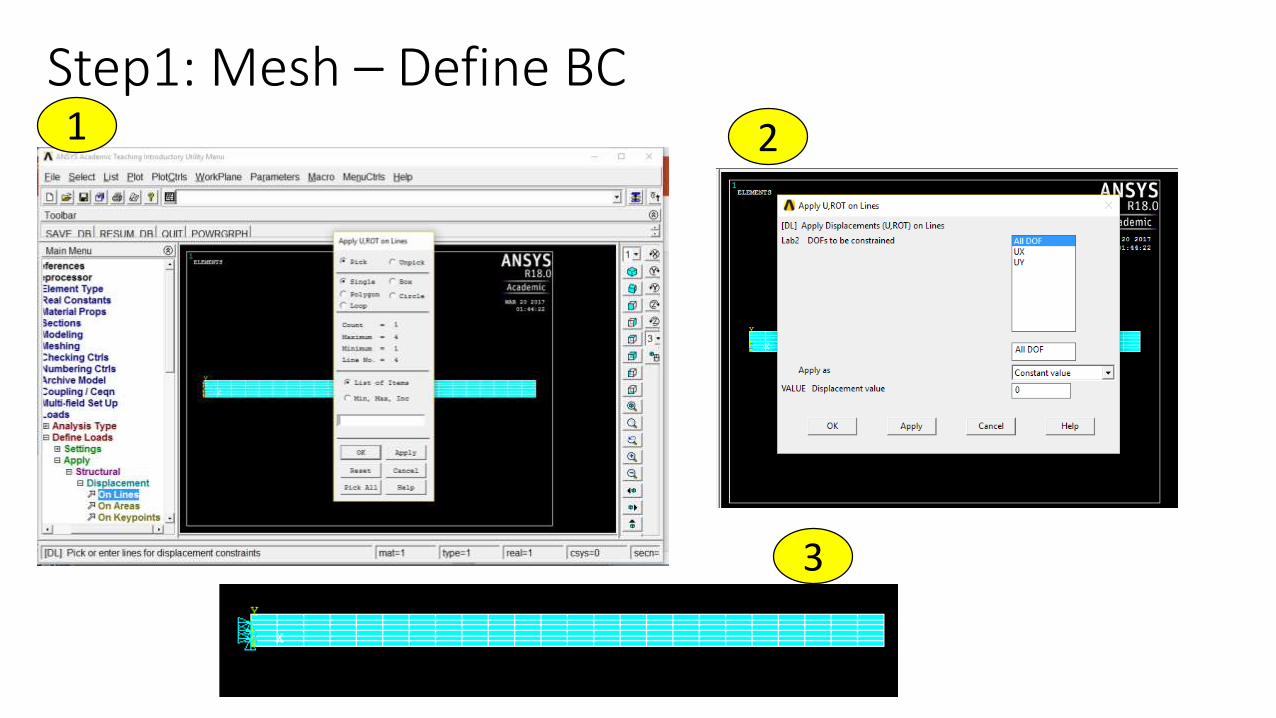
Step1: Mesh – Define BC1 2

3

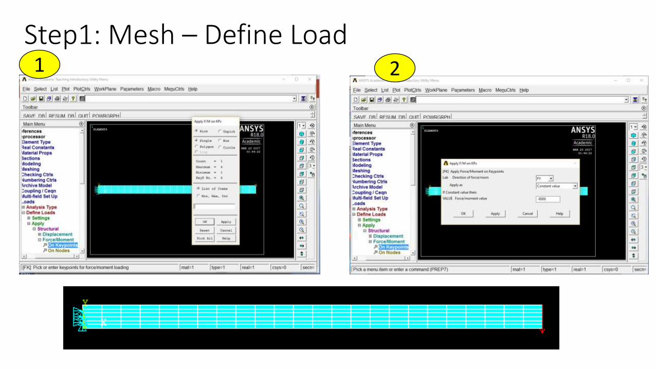
Step1: Mesh – Define Load1 2

Step1: Mesh – Solution

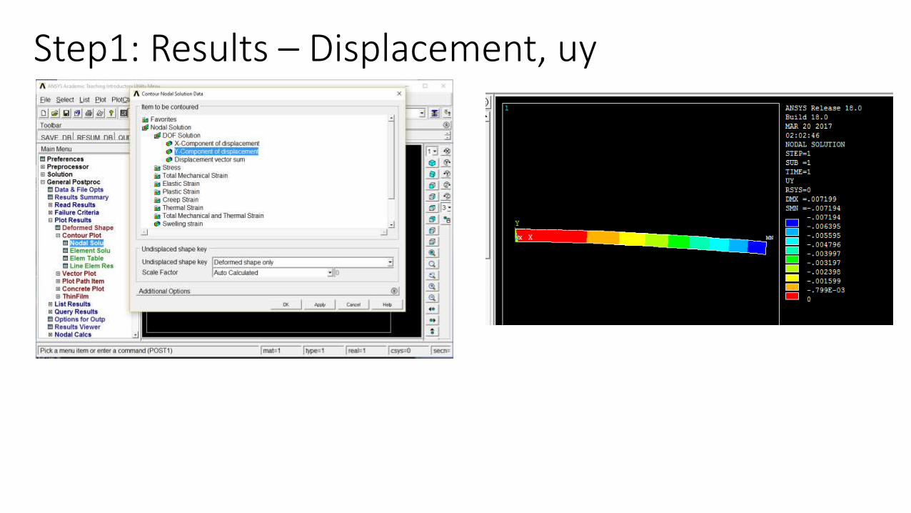
Step1: Results – Displacement, uy

Step1: Results – Stress, Sxx

Mesh Refinement: Spanner Stress Analysis

High Stress Region

Source: https://www.comsol.com/multiphysics/mesh-refinement

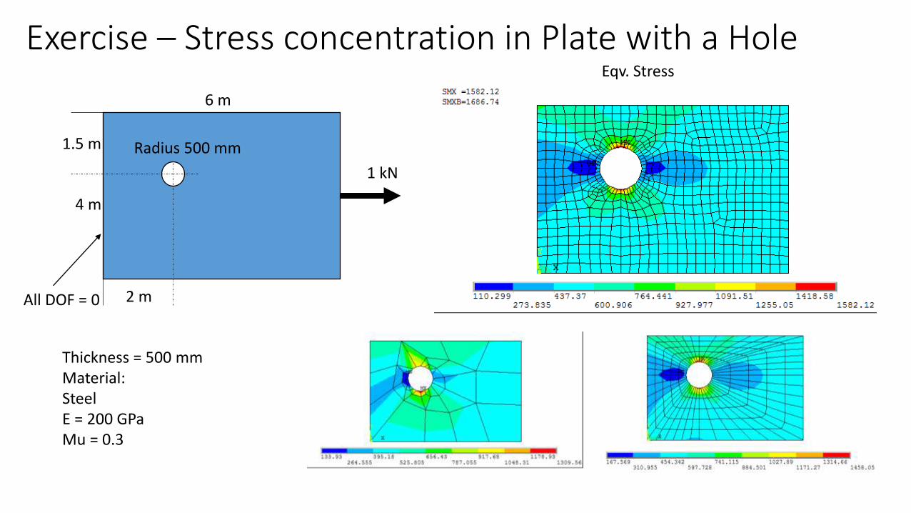
Exercise – Stress concentration in Plate with a Hole

1 kN

6 m

4 m

Radius 500 mm1.5 m

2 mAll DOF = 0

Thickness = 500 mmMaterial:SteelE = 200 GPaMu = 0.3

Eqv. Stress

Some common mistakes

• Inconsistent units• Wrong boundary conditions• Wrong material property assignment• Wrong element type assignment

Thank You

Documents

Introduction to Finite Element Analysis using ANSYS to Finite Element Analysis using ANSYS Sasi Kumar Tippabhotla PhD Candidate Xtreme Photovoltaics (XPV) Lab EPD, SUTD Disclaimer: