Embed Size (px)
Citation preview

STATISTICAL THINKING IN PYTHON I
Introduction to Exploratory Data
Analysis

Statistical Thinking in Python I
Exploratory data analysis
● The process of organizing, plo!ing, and summarizing a data set

Statistical Thinking in Python I
“Exploratory data analysis can never be the whole story, but nothing else can serve as the foundation stone.”
—John Tukey

Statistical Thinking in Python I
Data retrieved from Data.gov (h!ps://www.data.gov/)
2008 US swing state election results

Statistical Thinking in Python I
In [1]: import pandas as pd
In [2]: df_swing = pd.read_csv('2008_swing_states.csv')
In [3]: df_swing[['state', 'county', 'dem_share']] Out[3]: state county dem_share 0 PA Erie County 60.08 1 PA Bradford County 40.64 2 PA Tioga County 36.07 3 PA McKean County 41.21 4 PA Potter County 31.04 5 PA Wayne County 43.78 6 PA Susquehanna County 44.08 7 PA Warren County 46.85 8 OH Ashtabula County 56.94
2008 US swing state election results
Data retrieved from Data.gov (h!ps://www.data.gov/)

Statistical Thinking in Python I
Data retrieved from Data.gov (h!ps://www.data.gov/)
2008 US swing state election results

STATISTICAL THINKING IN PYTHON I
Let’s practice!

STATISTICAL THINKING IN PYTHON I
Plo!ing a histogram

Statistical Thinking in Python I
Data retrieved from Data.gov (h!ps://www.data.gov/)
2008 US swing state election results

Statistical Thinking in Python I
In [1]: import matplotlib.pyplot as plt
In [2]: _ = plt.hist(df_swing['dem_share'])
In [3]: _ = plt.xlabel('percent of vote for Obama')
In [4]: _ = plt.ylabel('number of counties')
In [5]: plt.show()
Generating a histogram

Statistical Thinking in Python I
● Always label your axes

Statistical Thinking in Python I
Data retrieved from Data.gov (h!ps://www.data.gov/)
2008 US swing state election results

Statistical Thinking in Python I
Data retrieved from Data.gov (h!ps://www.data.gov/)
Histograms with different binning

Statistical Thinking in Python I
In [1]: bin_edges = [0, 10, 20, 30, 40, 50, ...: 60, 70, 80, 90, 100]
In [2]: _ = plt.hist(df_swing['dem_share'], bins=bin_edges)
In [3]: plt.show()
Se!ing the bins of a histogram
Statistical Thinking in Python I
In [1]: _ = plt.hist(df_swing['dem_share'], bins=20)
In [2]: plt.show()
Se!ing the bins of a histogram

Statistical Thinking in Python I
Seaborn
● An excellent Matplotlib-based statistical data visualization package wri!en by Michael Waskom

Statistical Thinking in Python I
In [1]: import seaborn as sns
In [2]: sns.set()
In [3]: _ = plt.hist(df_swing['dem_share'])
In [4]: _ = plt.xlabel('percent of vote for Obama')
In [5]: _ = plt.ylabel('number of counties')
In [6]: plt.show()
Se!ing Seaborn styling

Statistical Thinking in Python I
Data retrieved from Data.gov (h!ps://www.data.gov/)
A Seaborn-styled histogram

STATISTICAL THINKING IN PYTHON I
Let’s practice!

STATISTICAL THINKING IN PYTHON I
Plot all of your data: Bee swarm plots

Statistical Thinking in Python I
Data retrieved from Data.gov (h!ps://www.data.gov/)
2008 US swing state election results

Statistical Thinking in Python I
Data retrieved from Data.gov (h!ps://www.data.gov/)
2008 US swing state election results

Statistical Thinking in Python I
Binning bias
● The same data may be interpreted differently depending on choice of bins

Statistical Thinking in Python I
Bee swarm plot
Data retrieved from Data.gov (h!ps://www.data.gov/)

Statistical Thinking in Python I
features of interest
observation
Organization of the data frame
Data retrieved from Data.gov (h!ps://www.data.gov/)
… … … … ………
state county total_votes dem_votes rep_votes dem_share 0 PA Erie County 127691 75775 50351 60.08 1 PA Bradford County 25787 10306 15057 40.64 2 PA Tioga County 17984 6390 11326 36.07 3 PA McKean County 15947 6465 9224 41.21 4 PA Potter County 7507 2300 5109 31.04 5 PA Wayne County 22835 9892 12702 43.78 6 PA Susquehanna County 19286 8381 10633 44.08 7 PA Warren County 18517 8537 9685 46.85 8 OH Ashtabula County 44874 25027 18949 56.94

Statistical Thinking in Python I
In [1]: _ = sns.swarmplot(x='state', y='dem_share', data=df_swing)
In [2]: _ = plt.xlabel('state')
In [3]: _ = plt.ylabel('percent of vote for Obama')
In [4]: plt.show()
Generating a bee swarm plot

Statistical Thinking in Python I
2008 US swing state election results
Data retrieved from Data.gov (h!ps://www.data.gov/)

STATISTICAL THINKING IN PYTHON I
Let’s practice!

STATISTICAL THINKING IN PYTHON I
Plot all of your data: ECDFs

Statistical Thinking in Python I
2008 US swing state election results
Data retrieved from Data.gov (h!ps://www.data.gov/)

Statistical Thinking in Python I
2008 US election results: East and West
Data retrieved from Data.gov (h!ps://www.data.gov/)

Statistical Thinking in Python I
Empirical cumulative distribution function (ECDF)
Data retrieved from Data.gov (h!ps://www.data.gov/)
20% of counties had36% or less vote for Obama
75% of counties hadless that half vote for Obama
Statistical Thinking in Python I
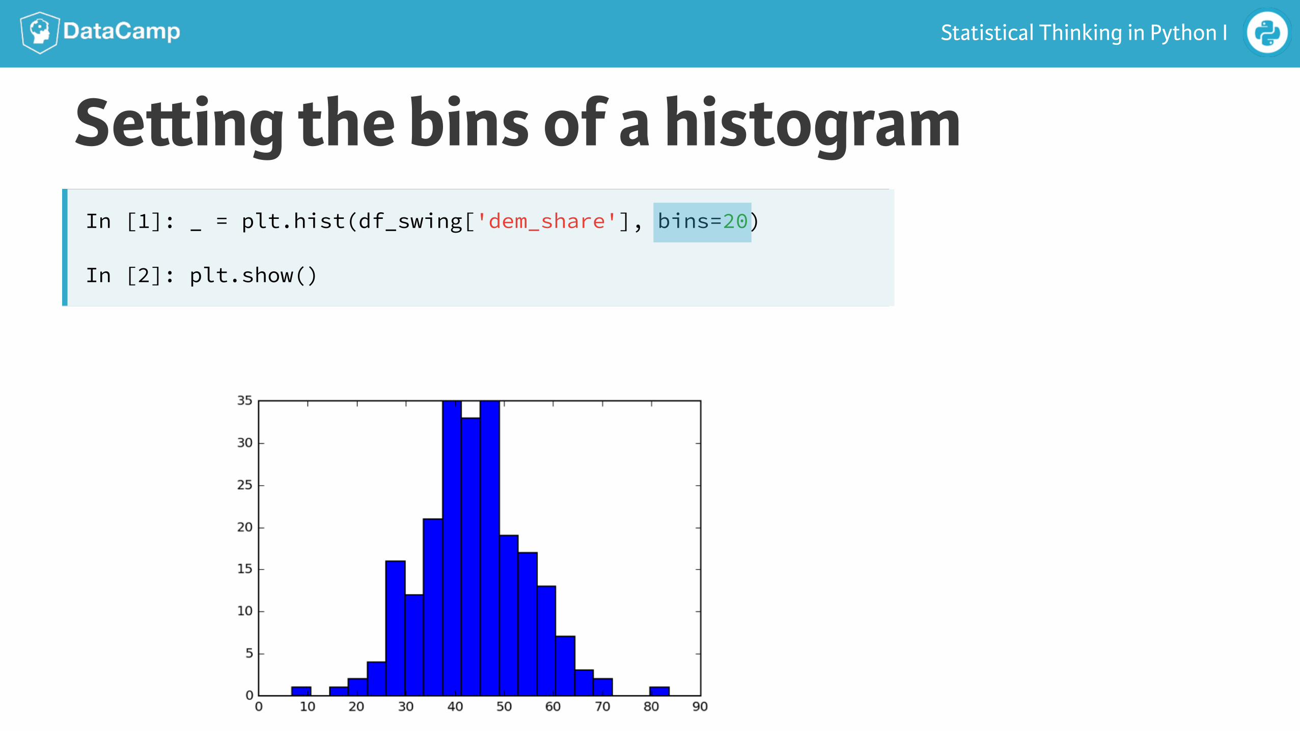
In [1]: import numpy as np
In [2]: x = np.sort(df_swing['dem_share'])
In [3]: y = np.arange(1, len(x)+1) / len(x)
In [4]: _ = plt.plot(x, y, marker='.', linestyle='none')
In [5]: _ = plt.xlabel('percent of vote for Obama')
In [6]: _ = plt.ylabel('ECDF')
In [7]: plt.margins(0.02) # Keeps data off plot edges
In [8]: plt.show()
Making an ECDF

Statistical Thinking in Python I
2008 US swing state election ECDF
Data retrieved from Data.gov (h!ps://www.data.gov/)

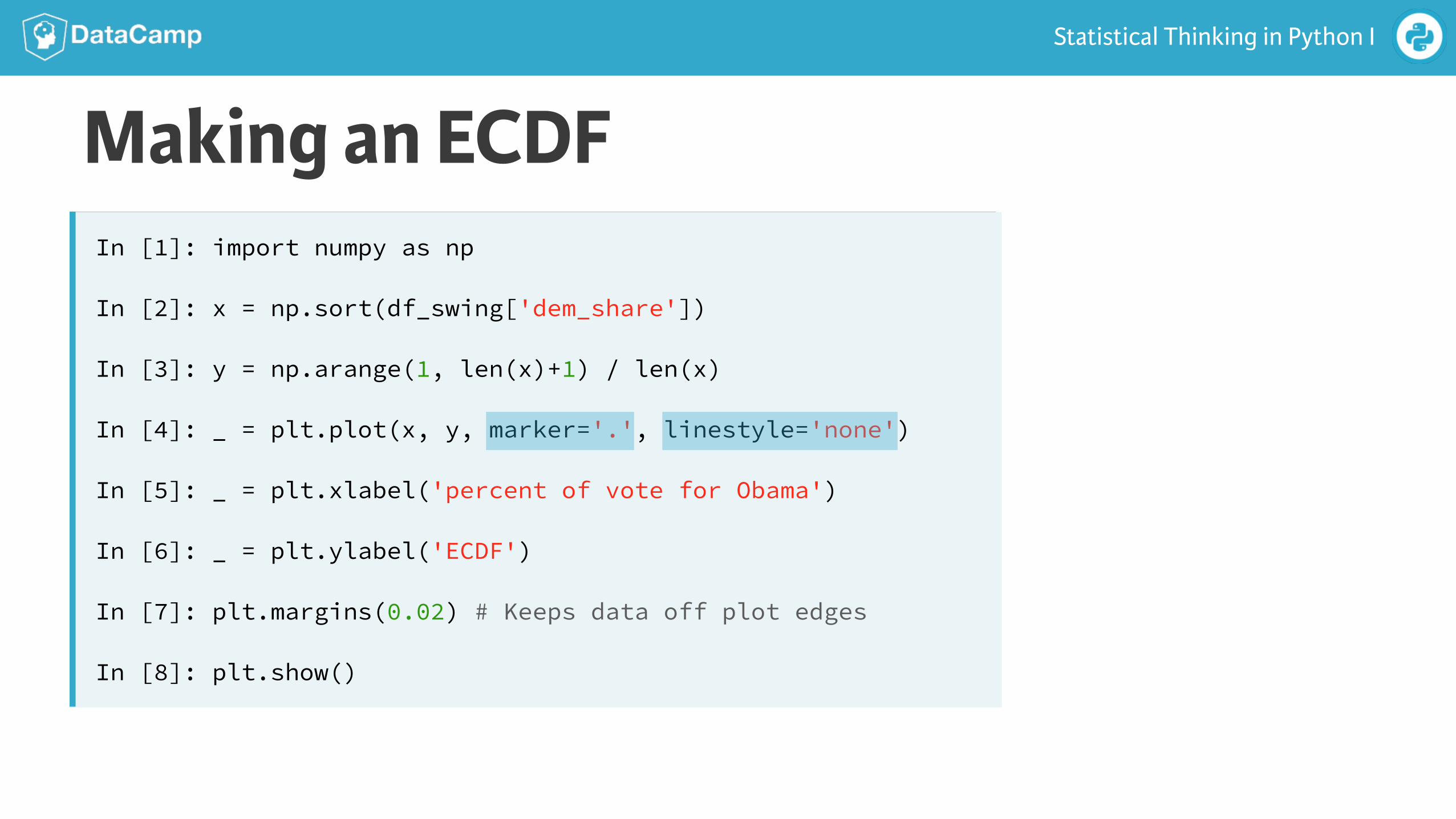
Statistical Thinking in Python I
Data retrieved from Data.gov (h!ps://www.data.gov/)
2008 US swing state election ECDFs

STATISTICAL THINKING IN PYTHON I
Let’s practice!

STATISTICAL THINKING IN PYTHON I
Onward toward the whole story!
Statistical Thinking in Python I

Statistical Thinking in Python I
“Exploratory data analysis can never be the whole story, but nothing else can serve as the foundation stone.”
—John Tukey

Statistical Thinking in Python I
Coming up…
● Thinking probabilistically
● Discrete and continuous distributions
● The power of hacker statistics using np.random()

STATISTICAL THINKING IN PYTHON I
Let’s get to work!