Embed Size (px)
Citation preview
1
CHAPTER 1
Introduction to EViews 10
CHAPTER OUTLINE Keywords 1.1 Using EViews for Principles of Econometrics,5E 1.1.1 Accessing and installing EViews 10 1.1.2 Obtaining data workfiles 1.1.3 Chapter 1 and the way forward 1.1.4 Font conventions 1.2 Starting and Exploring EViews 1.2.1 Creating a new workfile: workfile structures 1.2.2 Opening an existing workfile 1.2.3 The help system 1.3 Using a Workfile 1.3.1 Previewing series in the workfile 1.3.2 Examining a single series 1.3.3 Examing several series: a group 1.3.4 Freezing a result 1.3.5 Copying and pasting a table 1.3.6 Changing the sample 1.3.7 Generating a new series 1.3.8 EViews prompts 1.3.9 Saving the workfile 1.3.10 Snapshots 1.4 Using Commands 1.4.1 Command capture 1.4.2 Positioning the Command/Capture window 1.5 A Time-Series Workfile 1.5.1 Graphing a series 1.5.2 Copying a graph into a document 1.5.3 Changing the sample
1.5.4 Plotting two series 1.5.5 A scatter diagram 1.6 Using the Quick Menu 1.6.1 Using Sample from the Quick menu 1.6.2 Using Generate from the Quick menu 1.6.3 Using Show from the Quick menu 1.6.4 Creating a graph from the Quick menu 1.6.5 Opening an empty group 1.6.6 Quick/Series statistics 1.6.7 Quick/Group statistics 1.6.8 Other Quick menu items 1.7 Using the Object Menu 1.8 Using EViews Functions 1.8.1 Basic arithmetic operations 1.8.2 Basic math functions 1.8.3 Descriptive statistics functions 1.8.4 Saving commands in a text object 1.8.5 Using a storage vector 1.9 Creating and Manipulating Workfiles 1.9.1 Obtaining data from the Internet 1.9.2 Importing an Excel file 1.9.3 Importing other foreign files 1.9.4 Frequency conversions 1.9.5 Exporting data from EViews POE5 PROGRAMS POE5_CHAP01_UTOWN.PRG POE5_CHAP01_OZCONFN.PRG POE5_CHAP01_LONDON5.PRG
Keywords
@cor freeze preview series @mean frequency conversion Quick/Empty Group @round function reference Quick/Generate Series @sqrt generate series Quick/Graph
2 Chapter 1
@stdev genr Quick/Group Statistics @sum graph options Quick/Sample arithmetic operators grid lines Quick/Series Statistics basic graph group Quick/Showcommand window help samplecommon sample histogram and stats savecopying a table if condition scalarscopying a graph import Excel data scatter diagram correlation individual samples seriesCtrl+C internet data series: rename Ctrl+V line & symbol spreadsheet view data definition files math functions startup window data export multiple graphs text objectdata import name unstructured/undated data range new object vectordated-regular frequency object menu workfile structure descriptive statistics object name workfile: open EViews functions open group workfile: save EViews prompts open series workfilesframe & size path
1.1 USING EVIEWS FOR PRINCIPLES OF ECONOMETRICS, 5E
This manual is a supplement to the textbook Principles of Econometrics, 5th edition, by Hill, Griffiths and Lim (John Wiley & Sons, Inc., 2018). It is not in itself an econometrics book, nor is it a complete computer manual. Rather it is a step-by-step guide to using EViews 10 for the empirical examples in Principles of Econometrics, 5th edition, which we will abbreviate as POE5. We imagine you sitting at a computer with your POE5 text and Using EViews for Principles of Econometrics, 5th edition open, following along with the manual to replicate the examples in POE5. Before you can do so you must ensure you have access to EViews, either from a site license held by your university or by buying and installing your own personal copy. You will also need to obtain the EViews “workfiles” for POE5 which are the files that contain the data for the POE5 examples and exercises.
1.1.1 Accessing and installing EViews 10
If you plan to use EViews via a site license held by your university, your instructor will give you details about how to access EViews. It is, however, advantageous to own your own personal copy to ensure you have access when and where you want it, and to have your results from using EViews stored conveniently on your computer. If you plan to obtain your own copy of EViews, rather than relying totally on your university’s site license, there are three possible versions of EViews 10 you might like to consider. The home webpage for accessing details about a wide range of product versions of EViews is
www.eviews.com
The three versions likely to be of interest are (i) the Academic EViews 10 Standalone Edition for Windows, (ii) EViews 10 University Edition for Windows or Mac, and (iii) EViews 10 Student Version Lite for Windows or Mac. We recommend the University Edition.
Introduction to EViews 10 3
The Windows standalone version is the most powerful, but also the most expensive. For students of universities who have a site license, it is available at a greatly reduced price. The University Edition is only slightly less versatile than the standalone version and is more than adequate to handle all text examples and exercises in POE5. Its license expires after six months; it is only available to enrolled students. The Student Version Lite is free, but it has the severe disadvantage that results cannot be saved for future use when the EViews workfile is closed. It also has limits on the numbers of series and observations, and it does not accept EViews programs. Its license expires after one year. Both the University Edition and the Student Version Lite require connection to the Internet once every 10 days. A full comparison of the three versions and instructions for purchasing/downloading can be found at
www.eviews.com/EViews10/EViews10Univ/evuniv10.html
For details of all EViews academic licenses, go to
www.eviews.com/BuyNow/Academic.html
Once you have downloaded EViews you can install it by double clicking on the EViews Installer .exe file, and following the prompts. When EViews is started – see the next section – you will be prompted to register EViews on your computer using a serial number provided to you. For the various steps and instructions that we describe, we are following Windows conventions.
1.1.2 Obtaining data workfiles
The EViews data workfiles (with extension *.wf1) and other resources for POE5 can be found at principlesofeconometrics.com/poe5/poe5.html. In addition to the EViews workfiles, there are data definition files (*.def) that describe the variables and show some summary statistics. The definition files are simple text files that can be opened with utilities like Notepad or Wordpad, or using a word processor. These files should be downloaded as well.
1.1.3 Chapter 1 and the way forward
Except for Chapter 1, the chapters in this manual correspond to chapters in POE5. From Chapter 2 onwards, we describe how to use EViews to replicate the empirical examples in POE5. We also include EViews instructions for the Monte Carlo simulations that appear in some of POE5’s chapter appendices. Appendices A, B and C at the end of this manual correspond to the same book appendices in POE5. They are a useful resource, explaing many of the EViews functions.
In Chapter 1 we introduce you to some of the basic features of EViews. Learning these features will save you time when you embark on the examples in the remaining chapters. However, Chapter 1 is a long chapter. You are unlikely to remember everything in it. You may wish to read it selectively, reserving some sections as a reference to which you can return later. Many of the instructions in Chapter 1 are repeated in later chapters, for reinforcement, and in recognition that not all students, particularly those who are already have some familiarity with EViews, will begin their POE5-EViews adventure at a later chapter.
4 Chapter 1
1.1.4 Font conventions
Throughout this manual we have adopted several font conventions for referring to various objects, EViews commands, and items in pull-down menus and toolbars. Here is a summary of those conventions. This summary is unlikely to be meaningful to you at this time, but it can be used for later reference.
File names and programs: times new Roman, lower case, italic, bold; e.g., utown.wf1.
Series: times new Roman, upper case, italic; e.g., PRICE.
Other workfile objects: arial, lower case, bold; e.g., house_data
Pull-down menus, toolbar items and dialog boxes: times new Roman, first letter upper case, bold; e.g., Genr and Quick/Series Statistics/Histogram and Stats
Commands for the command window: indented new line, arial, lower case, bold; e.g.,
series dinc = inc – inc(-1)
1.2 STARTING AND EXPLORING EVIEWS
If you have installed EViews by following the default prompts, the EViews 10 icon will appear on your desktop. It should resemble
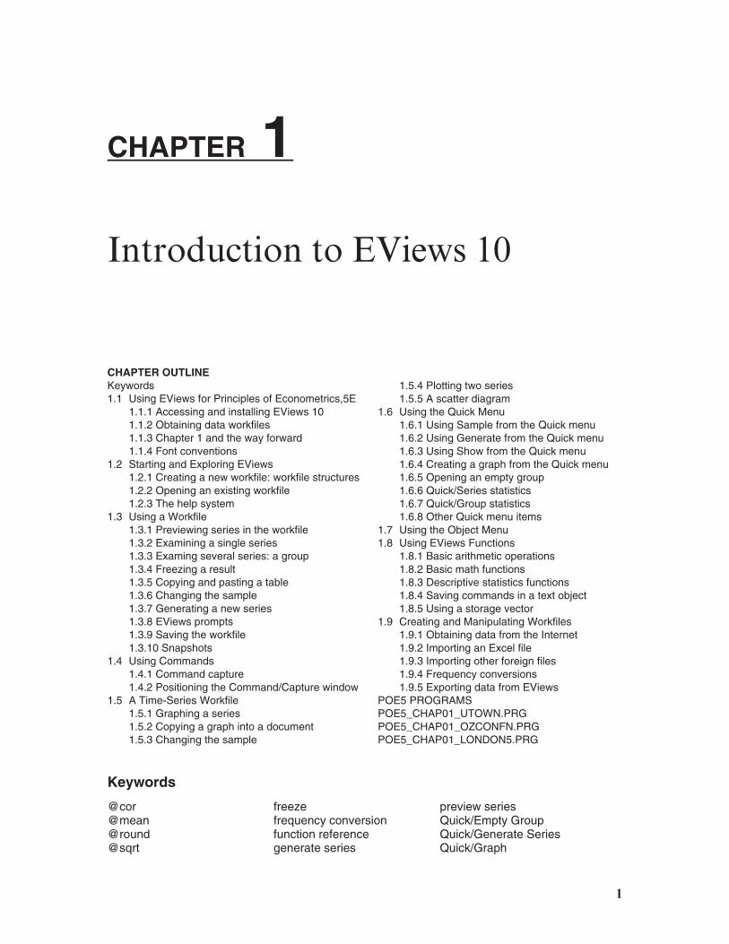
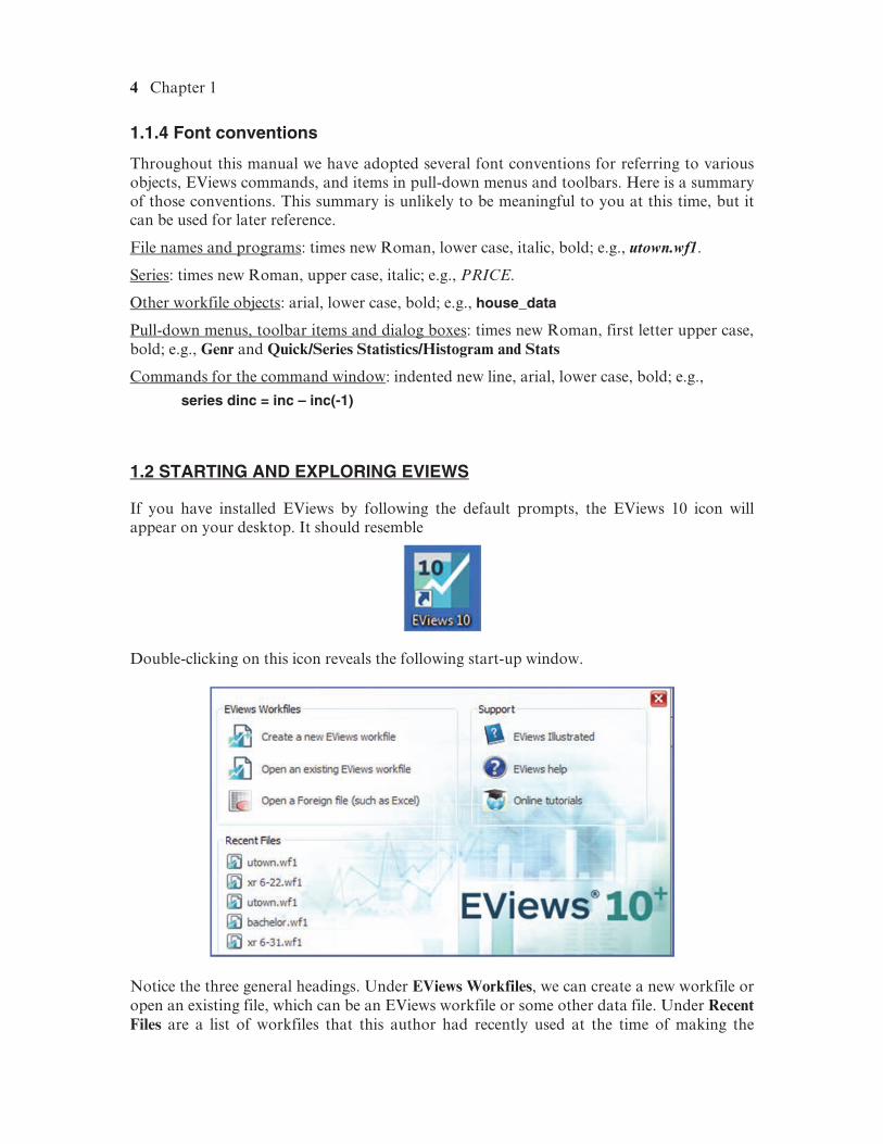
Double-clicking on this icon reveals the following start-up window.
Notice the three general headings. Under EViews Workfiles, we can create a new workfile or open an existing file, which can be an EViews workfile or some other data file. Under Recent Files are a list of workfiles that this author had recently used at the time of making the
Introduction to EViews 10 5
screenshot. Clicking on the name of one of these workfiles will open it. Under Support are three ways of getting help, each of which can be accessed by clicking on the relevant item.
Let’s examine some of these things in more detail.
1.2.1 Creating a new workfile: workfile structures
If you plan to use only the POE5 EViews workfiles, or workfiles provided from some other source, then you will not need to create a new workfile; you can focus on instructions for opening an existing workfile. In POE5, creation of new workfiles is limited to the Monte Carlo simulations, graphing of functions in Appendix A, and illustrating probability distributions in Appendix B. However, it is convenient at this point to consider how to create a new workfile to introduce you to EViews workfile structures.
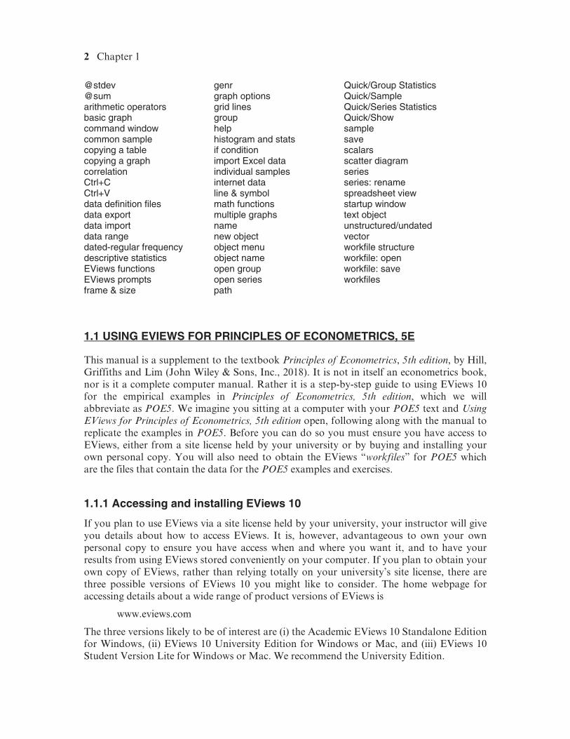
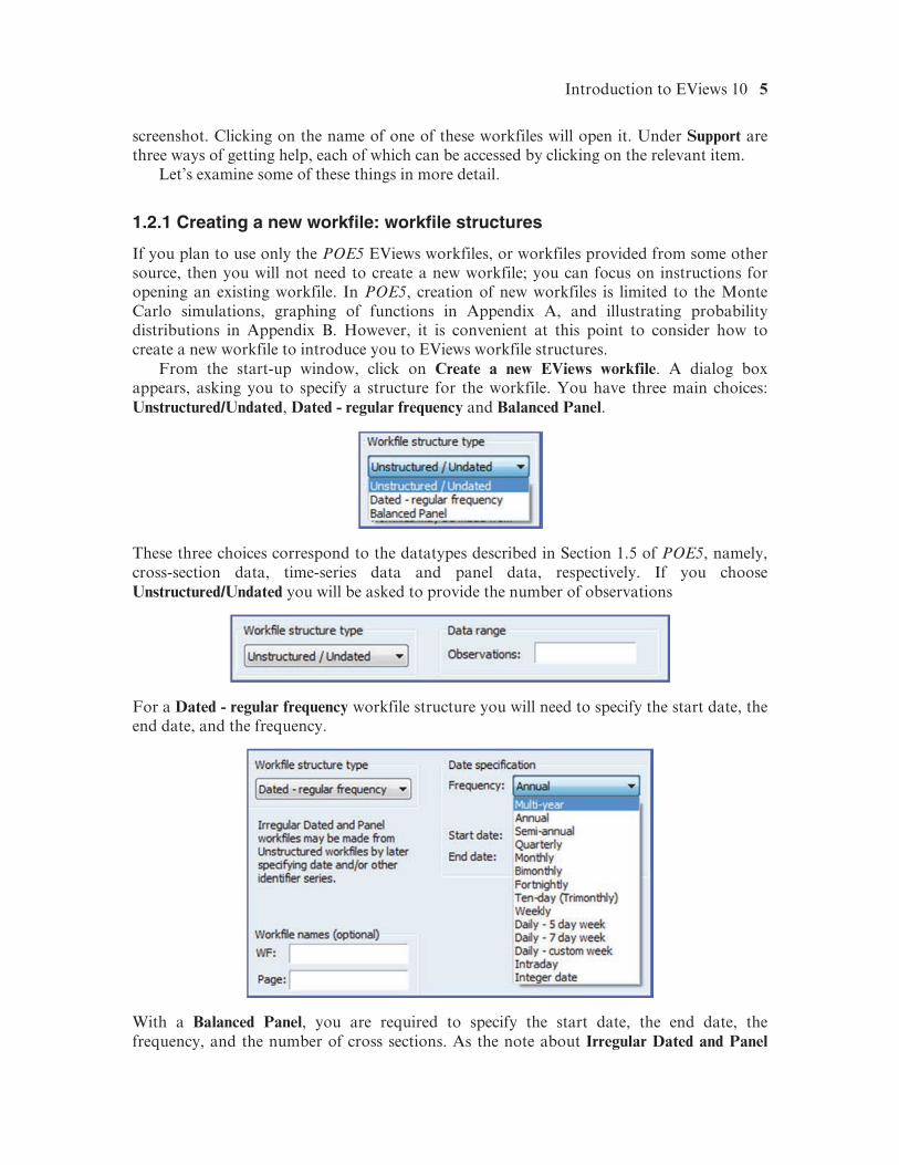
From the start-up window, click on Create a new EViews workfile. A dialog box appears, asking you to specify a structure for the workfile. You have three main choices: Unstructured/Undated, Dated - regular frequency and Balanced Panel.
These three choices correspond to the datatypes described in Section 1.5 of POE5, namely, cross-section data, time-series data and panel data, respectively. If you choose Unstructured/Undated you will be asked to provide the number of observations
For a Dated - regular frequency workfile structure you will need to specify the start date, the end date, and the frequency.
With a Balanced Panel, you are required to specify the start date, the end date, the frequency, and the number of cross sections. As the note about Irregular Dated and Panel
6 Chapter 1
workfiles suggests, more complex structures such as irregular frequencies or unbalanced panels are possible, but it is too early in the book for us to consider such complications.
The remaining request for information in the start-up window is for a workfile name and a page name. EViews has capacity for using multiple pages with different structures within the same workfile. This facility can be useful for different types of calculations, but we will almost always use just a single page.
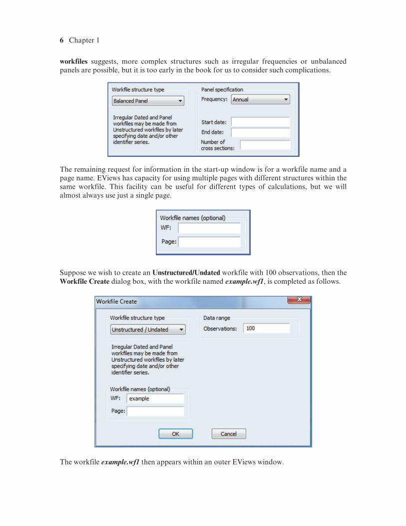
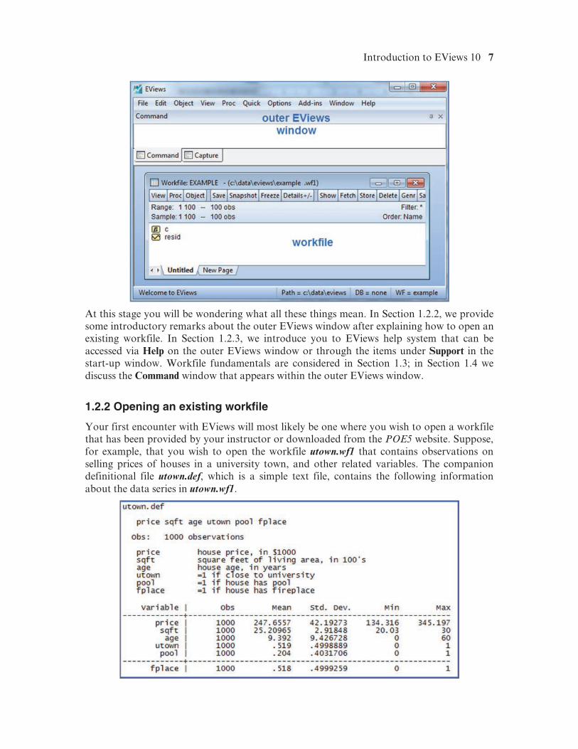
Suppose we wish to create an Unstructured/Undated workfile with 100 observations, then the Workfile Create dialog box, with the workfile named example.wf1, is completed as follows.
The workfile example.wf1 then appears within an outer EViews window.
Introduction to EViews 10 7
At this stage you will be wondering what all these things mean. In Section 1.2.2, we provide some introductory remarks about the outer EViews window after explaining how to open an existing workfile. In Section 1.2.3, we introduce you to EViews help system that can be accessed via Help on the outer EViews window or through the items under Support in the start-up window. Workfile fundamentals are considered in Section 1.3; in Section 1.4 we discuss the Command window that appears within the outer EViews window.
1.2.2 Opening an existing workfile
Your first encounter with EViews will most likely be one where you wish to open a workfile that has been provided by your instructor or downloaded from the POE5 website. Suppose, for example, that you wish to open the workfile utown.wf1 that contains observations on selling prices of houses in a university town, and other related variables. The companion definitional file utown.def, which is a simple text file, contains the following information about the data series in utown.wf1.
8 Chapter 1
These details are self-explanatory except perhaps for the binary (dummy) variables UTOWN, POOL and FIREPLACE which are equal to 1 if a house has the specified characteristic, and zero otherwise.
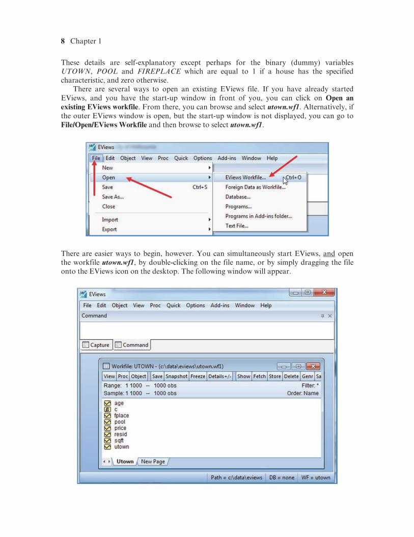
There are several ways to open an existing EViews file. If you have already started EViews, and you have the start-up window in front of you, you can click on Open an existing EViews workfile. From there, you can browse and select utown.wf1. Alternatively, if the outer EViews window is open, but the start-up window is not displayed, you can go to File/Open/EViews Workfile and then browse to select utown.wf1.
There are easier ways to begin, however. You can simultaneously start EViews, and open the workfile utown.wf1, by double-clicking on the file name, or by simply dragging the file onto the EViews icon on the desktop. The following window will appear.
Introduction to EViews 10 9
The inner window headed
is the workfile. It sits within the EViews software outer window which is headed
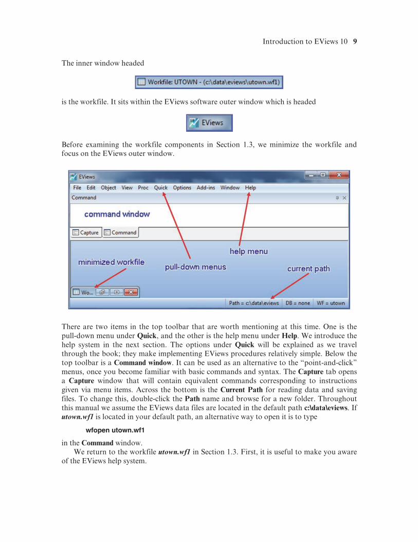
Before examining the workfile components in Section 1.3, we minimize the workfile and focus on the EViews outer window.
There are two items in the top toolbar that are worth mentioning at this time. One is the pull-down menu under Quick, and the other is the help menu under Help. We introduce the help system in the next section. The options under Quick will be explained as we travel through the book; they make implementing EViews procedures relatively simple. Below the top toolbar is a Command window. It can be used as an alternative to the “point-and-click” menus, once you become familiar with basic commands and syntax. The Capture tab opens a Capture window that will contain equivalent commands corresponding to instructions given via menu items. Across the bottom is the Current Path for reading data and saving files. To change this, double-click the Path name and browse for a new folder. Throughout this manual we assume the EViews data files are located in the default path c:\data\eviews. If utown.wf1 is located in your default path, an alternative way to open it is to type
wfopen utown.wf1
in the Command window. We return to the workfile utown.wf1 in Section 1.3. First, it is useful to make you aware
of the EViews help system.
10 Chapter 1
1.2.3 The help system
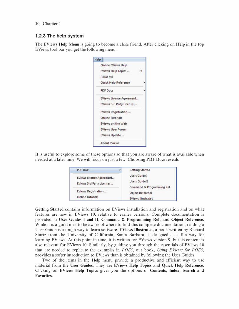
The EViews Help Menu is going to become a close friend. After clicking on Help in the top EViews tool bar you get the following menu.
It is useful to explore some of these options so that you are aware of what is available when needed at a later time. We will focus on just a few. Choosing PDF Docs reveals
Getting Started contains information on EViews installation and registration and on what features are new in EViews 10, relative to earlier versions. Complete documentation is provided in User Guides I and II, Command & Programming Ref, and Object Reference. While it is a good idea to be aware of where to find this complete documentation, reading a User Guide is a tough way to learn software. EViews Illustrated, a book written by Richard Startz from the University of California, Santa Barbara, is designed as a fun way for learning EViews. At this point in time, it is written for EViews version 9, but its content is also relevant for EViews 10. Similarly, by guiding you through the essentials of EViews 10 that are needed to replicate the examples in POE5, our book, Using EViews for POE5, provides a softer introduction to EViews than is obtained by following the User Guides.
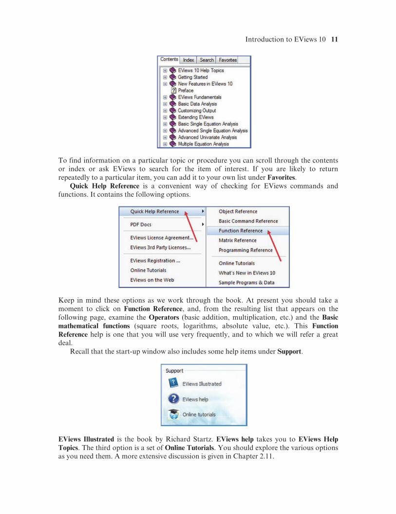
Two of the items in the Help menu provide a productive and efficient way to use material from the User Guides. They are EViews Help Topics and Quick Help Reference. Clicking on EViews Help Topics gives you the options of Contents, Index, Search and Favorites.
Introduction to EViews 10 11
To find information on a particular topic or procedure you can scroll through the contents or index or ask EViews to search for the item of interest. If you are likely to return repeatedly to a particular item, you can add it to your own list under Favorites.
Quick Help Reference is a convenient way of checking for EViews commands and functions. It contains the following options.
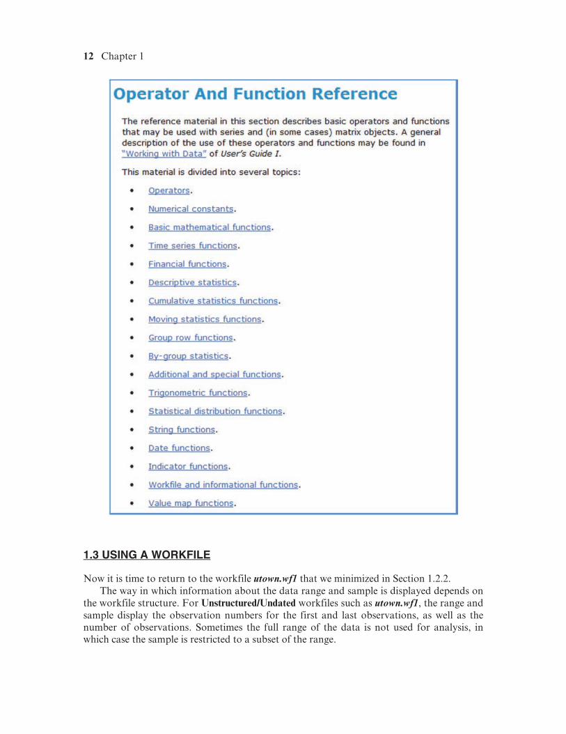
Keep in mind these options as we work through the book. At present you should take a moment to click on Function Reference, and, from the resulting list that appears on the following page, examine the Operators (basic addition, multiplication, etc.) and the Basic mathematical functions (square roots, logarithms, absolute value, etc.). This Function Reference help is one that you will use very frequently, and to which we will refer a great deal.
Recall that the start-up window also includes some help items under Support.
EViews Illustrated is the book by Richard Startz. EViews help takes you to EViews Help Topics. The third option is a set of Online Tutorials. You should explore the various options as you need them. A more extensive discussion is given in Chapter 2.11.
12 Chapter 1
1.3 USING A WORKFILE
Now it is time to return to the workfile utown.wf1 that we minimized in Section 1.2.2. The way in which information about the data range and sample is displayed depends on
the workfile structure. For Unstructured/Undated workfiles such as utown.wf1, the range and sample display the observation numbers for the first and last observations, as well as the number of observations. Sometimes the full range of the data is not used for analysis, in which case the sample is restricted to a subset of the range.
Introduction to EViews 10 13
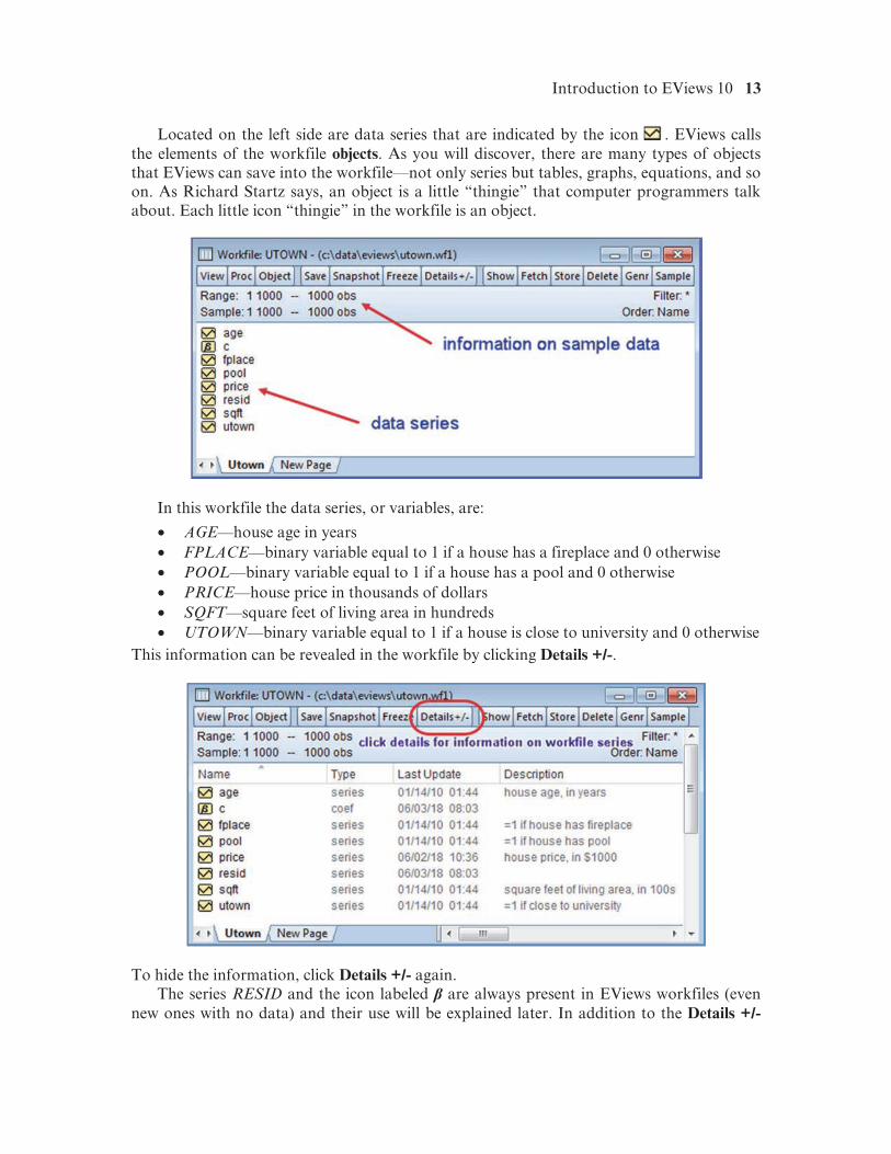
Located on the left side are data series that are indicated by the icon . EViews calls the elements of the workfile objects. As you will discover, there are many types of objects that EViews can save into the workfile—not only series but tables, graphs, equations, and so on. As Richard Startz says, an object is a little “thingie” that computer programmers talk about. Each little icon “thingie” in the workfile is an object.
In this workfile the data series, or variables, are:
• AGE—house age in years • FPLACE—binary variable equal to 1 if a house has a fireplace and 0 otherwise • POOL—binary variable equal to 1 if a house has a pool and 0 otherwise • PRICE—house price in thousands of dollars • SQFT—square feet of living area in hundreds • UTOWN—binary variable equal to 1 if a house is close to university and 0 otherwise
This information can be revealed in the workfile by clicking Details +/-.
To hide the information, click Details +/- again. The series RESID and the icon labeled are always present in EViews workfiles (even
new ones with no data) and their use will be explained later. In addition to the Details +/-
14 Chapter 1
button, across the top of the workfile are various buttons that initiate tasks in EViews; these too will be explained later.
1.3.1 Previewing series in the workfile
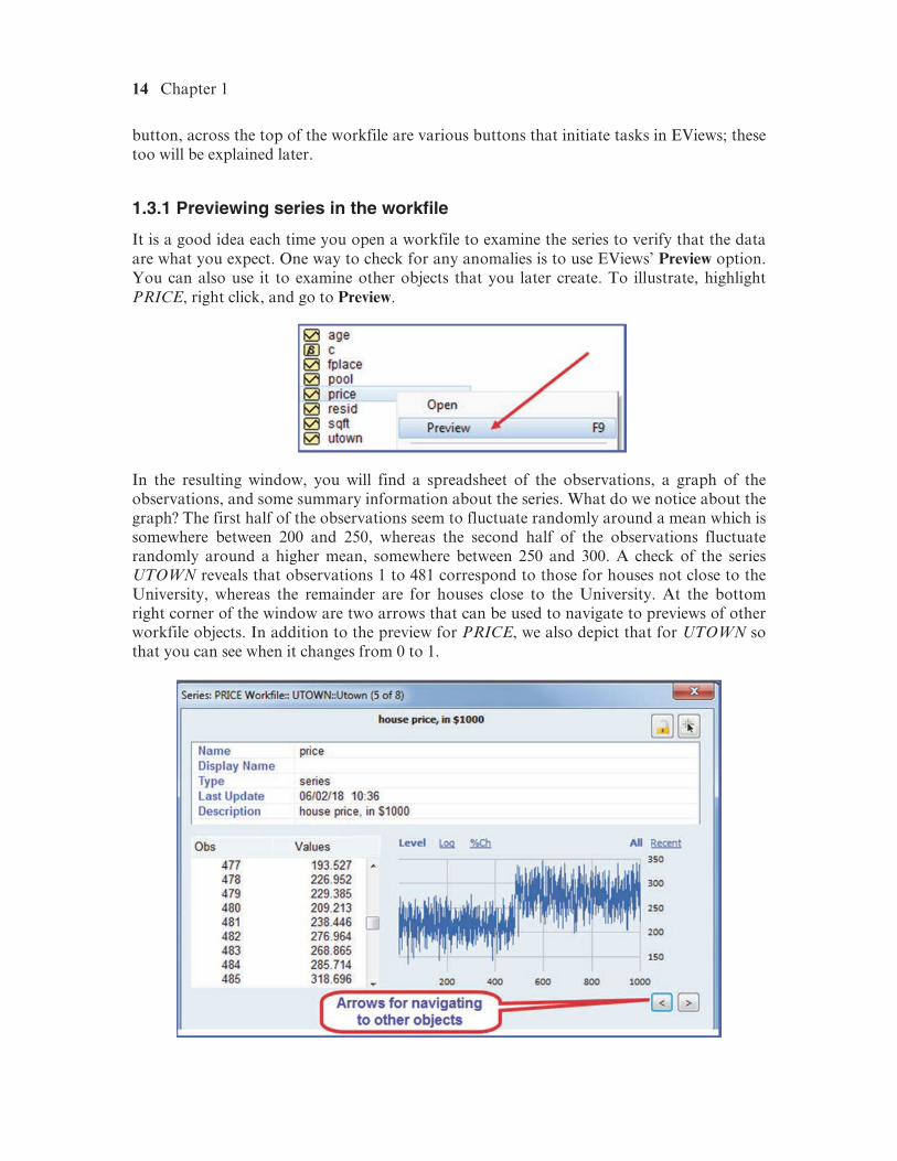
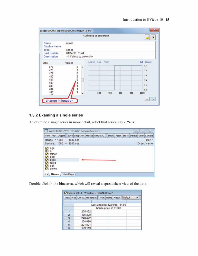
It is a good idea each time you open a workfile to examine the series to verify that the data are what you expect. One way to check for any anomalies is to use EViews’ Preview option. You can also use it to examine other objects that you later create. To illustrate, highlight PRICE, right click, and go to Preview.
In the resulting window, you will find a spreadsheet of the observations, a graph of the observations, and some summary information about the series. What do we notice about the graph? The first half of the observations seem to fluctuate randomly around a mean which is somewhere between 200 and 250, whereas the second half of the observations fluctuate randomly around a higher mean, somewhere between 250 and 300. A check of the series UTOWN reveals that observations 1 to 481 correspond to those for houses not close to the University, whereas the remainder are for houses close to the University. At the bottom right corner of the window are two arrows that can be used to navigate to previews of other workfile objects. In addition to the preview for PRICE, we also depict that for UTOWN so that you can see when it changes from 0 to 1.
Introduction to EViews 10 15
1.3.2 Examing a single series
To examine a single series in more detail, select that series, say PRICE
Double-click in the blue area, which will reveal a spreadsheet view of the data.
16 Chapter 1
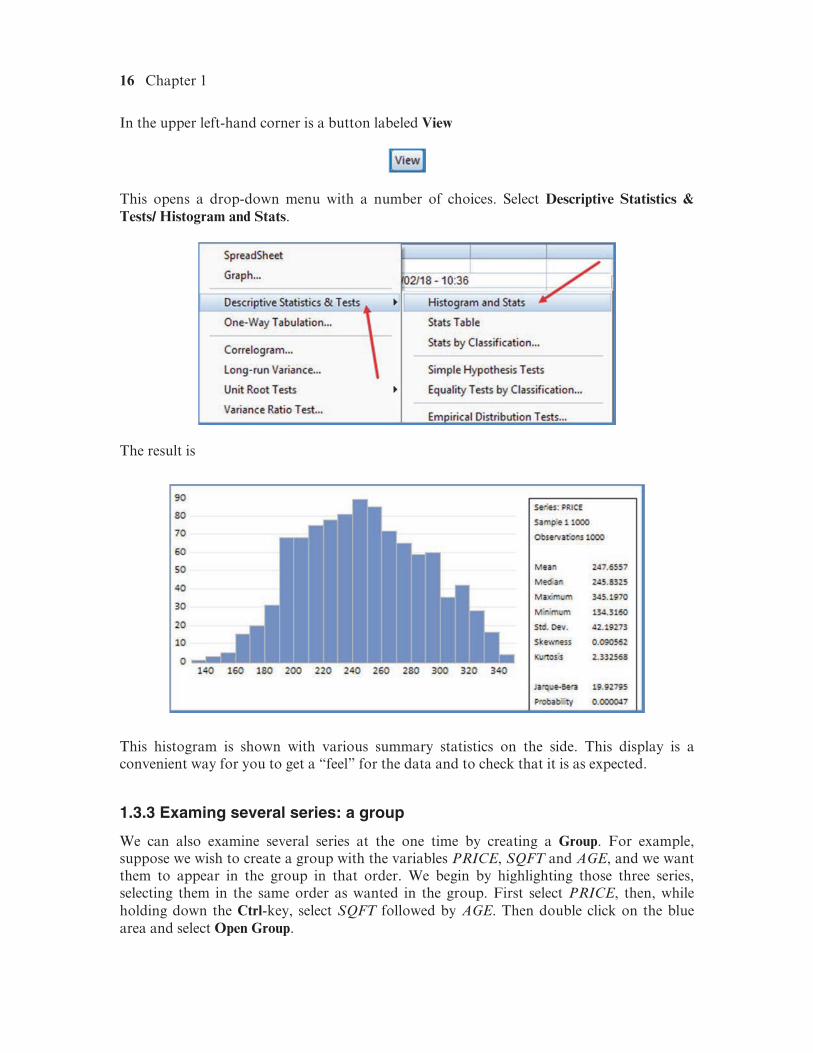
In the upper left-hand corner is a button labeled View
This opens a drop-down menu with a number of choices. Select Descriptive Statistics & Tests/ Histogram and Stats.
The result is
This histogram is shown with various summary statistics on the side. This display is a convenient way for you to get a “feel” for the data and to check that it is as expected.
1.3.3 Examing several series: a group
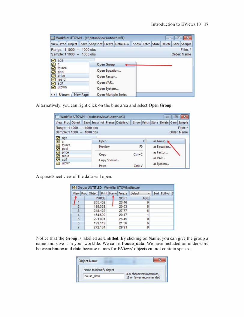
We can also examine several series at the one time by creating a Group. For example, suppose we wish to create a group with the variables PRICE, SQFT and AGE, and we want them to appear in the group in that order. We begin by highlighting those three series, selecting them in the same order as wanted in the group. First select PRICE, then, while holding down the Ctrl-key, select SQFT followed by AGE. Then double click on the blue area and select Open Group.
Introduction to EViews 10 17
Alternatively, you can right click on the blue area and select Open Group.
A spreadsheet view of the data will open.
Notice that the Group is labelled as Untitled. By clicking on Name, you can give the group a name and save it in your workfile. We call it house_data. We have included an underscore between house and data because names for EViews’ objects cannot contain spaces.
18 Chapter 1
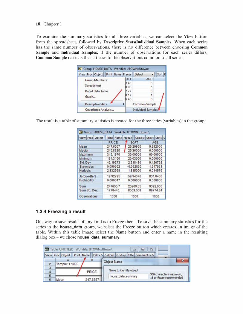
To examine the summary statistics for all three variables, we can select the View button from the spreadsheet, followed by Descriptive Stats/Individual Samples. When each series has the same number of observations, there is no difference between choosing Common Sample and Individual Samples; if the number of observations for each series differs, Common Sample restricts the statistics to the observations common to all series.
The result is a table of summary statistics is created for the three series (variables) in the group.
1.3.4 Freezing a result
One way to save results of any kind is to Freeze them. To save the summary statistics for the series in the house_data group, we select the Freeze button which creates an image of the table. Within this table image, select the Name button and enter a name in the resulting dialog box – we chose house_data_summary.
Introduction to EViews 10 19
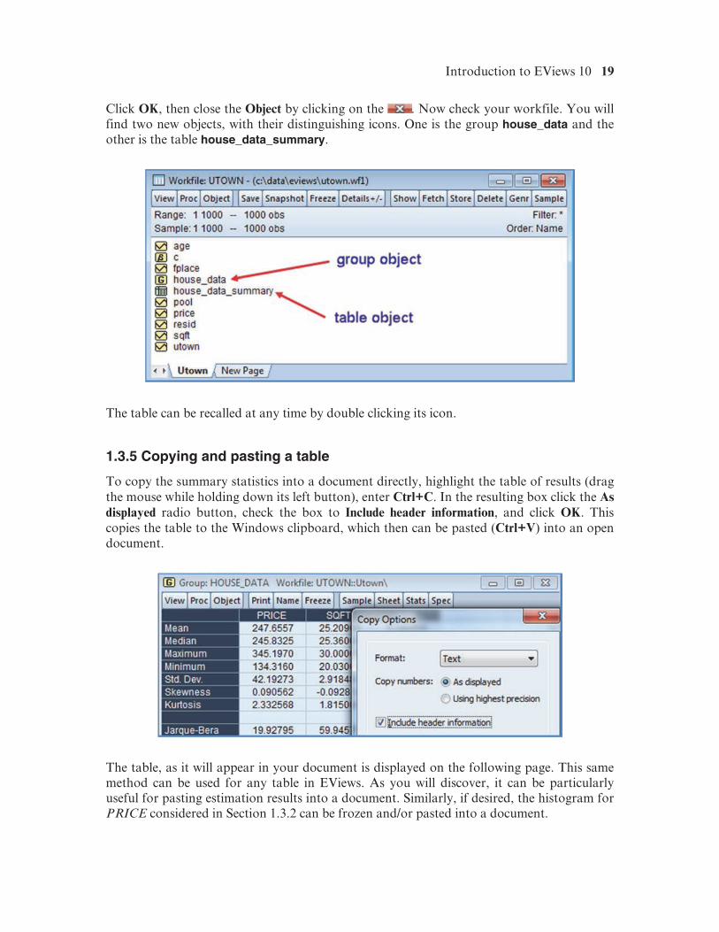
Click OK, then close the Object by clicking on the . Now check your workfile. You will find two new objects, with their distinguishing icons. One is the group house_data and the other is the table house_data_summary.
The table can be recalled at any time by double clicking its icon.
1.3.5 Copying and pasting a table
To copy the summary statistics into a document directly, highlight the table of results (drag the mouse while holding down its left button), enter Ctrl+C. In the resulting box click the As displayed radio button, check the box to Include header information, and click OK. This copies the table to the Windows clipboard, which then can be pasted (Ctrl+V) into an open document.
The table, as it will appear in your document is displayed on the following page. This same method can be used for any table in EViews. As you will discover, it can be particularly useful for pasting estimation results into a document. Similarly, if desired, the histogram for PRICE considered in Section 1.3.2 can be frozen and/or pasted into a document.
20 Chapter 1
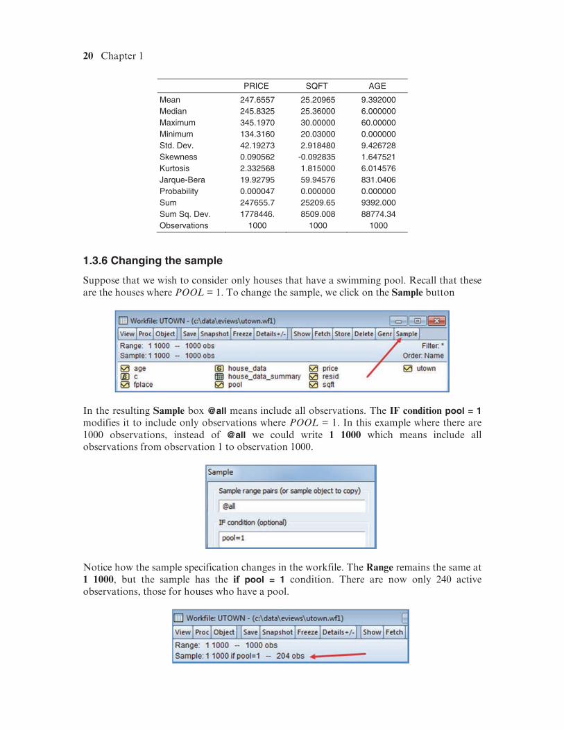
PRICE SQFT AGE
Mean 247.6557 25.20965 9.392000 Median 245.8325 25.36000 6.000000 Maximum 345.1970 30.00000 60.00000 Minimum 134.3160 20.03000 0.000000 Std. Dev. 42.19273 2.918480 9.426728 Skewness 0.090562 -0.092835 1.647521 Kurtosis 2.332568 1.815000 6.014576 Jarque-Bera 19.92795 59.94576 831.0406 Probability 0.000047 0.000000 0.000000 Sum 247655.7 25209.65 9392.000 Sum Sq. Dev. 1778446. 8509.008 88774.34 Observations 1000 1000 1000
1.3.6 Changing the sample
Suppose that we wish to consider only houses that have a swimming pool. Recall that these are the houses where POOL = 1. To change the sample, we click on the Sample button
In the resulting Sample box @all means include all observations. The IF condition pool = 1 modifies it to include only observations where POOL = 1. In this example where there are 1000 observations, instead of @all we could write 1 1000 which means include all observations from observation 1 to observation 1000.
Notice how the sample specification changes in the workfile. The Range remains the same at 1 1000, but the sample has the if pool = 1 condition. There are now only 240 active observations, those for houses who have a pool.
Introduction to EViews 10 21
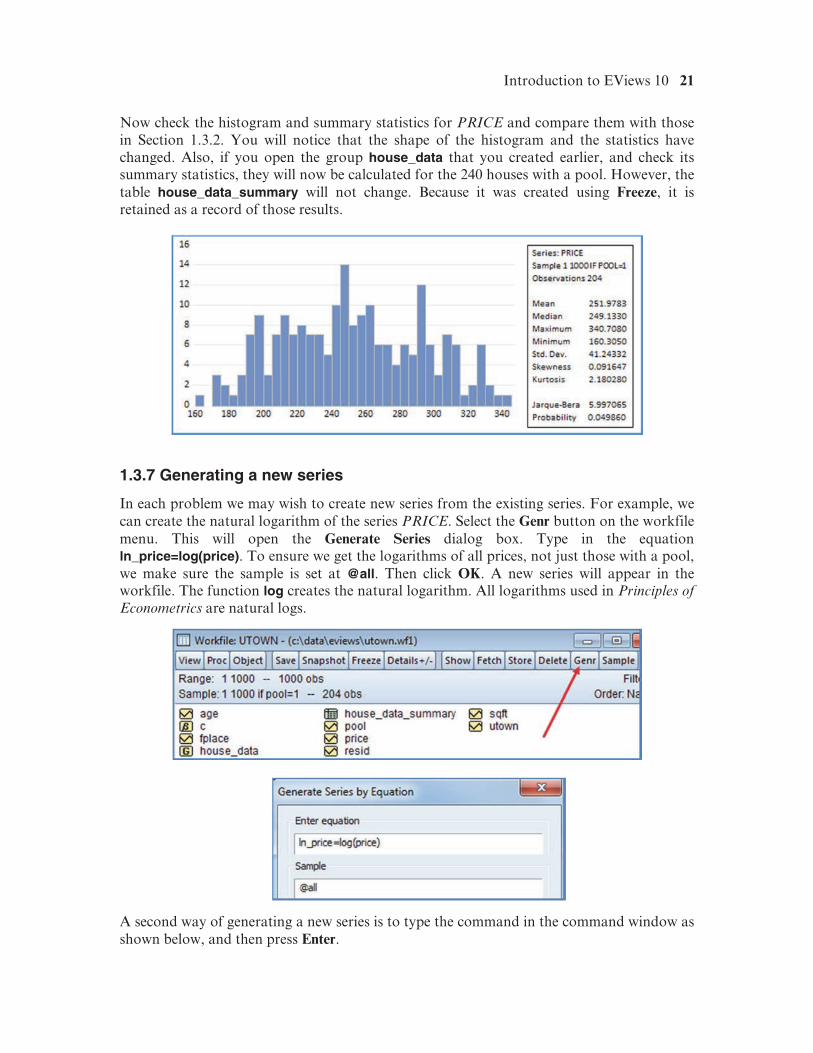
Now check the histogram and summary statistics for PRICE and compare them with those in Section 1.3.2. You will notice that the shape of the histogram and the statistics have changed. Also, if you open the group house_data that you created earlier, and check its summary statistics, they will now be calculated for the 240 houses with a pool. However, the table house_data_summary will not change. Because it was created using Freeze, it is retained as a record of those results.
1.3.7 Generating a new series
In each problem we may wish to create new series from the existing series. For example, we can create the natural logarithm of the series PRICE. Select the Genr button on the workfile menu. This will open the Generate Series dialog box. Type in the equation ln_price=log(price). To ensure we get the logarithms of all prices, not just those with a pool, we make sure the sample is set at @all. Then click OK. A new series will appear in the workfile. The function log creates the natural logarithm. All logarithms used in Principles of Econometrics are natural logs.
A second way of generating a new series is to type the command in the command window as shown below, and then press Enter.
22 Chapter 1
The command series creates the new series. It is also possible to write
genr ln_price=log(price)
As we travel through the book, we will discover how to use a number of commands as an alternative to pointing and clicking.
1.3.8 EViews prompts
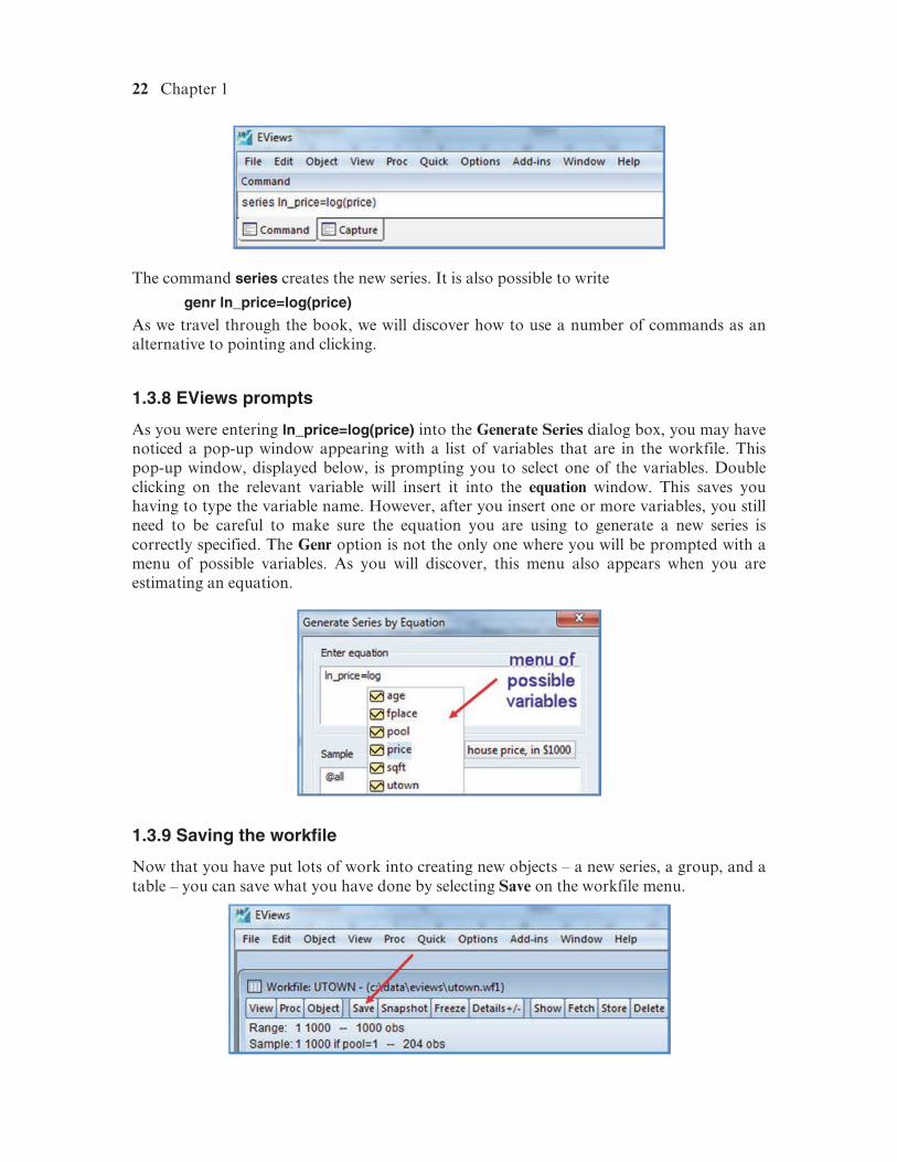
As you were entering ln_price=log(price) into the Generate Series dialog box, you may have noticed a pop-up window appearing with a list of variables that are in the workfile. This pop-up window, displayed below, is prompting you to select one of the variables. Double clicking on the relevant variable will insert it into the equation window. This saves you having to type the variable name. However, after you insert one or more variables, you still need to be careful to make sure the equation you are using to generate a new series is correctly specified. The Genr option is not the only one where you will be prompted with a menu of possible variables. As you will discover, this menu also appears when you are estimating an equation.
1.3.9 Saving the workfile
Now that you have put lots of work into creating new objects – a new series, a group, and a table – you can save what you have done by selecting Save on the workfile menu.
Introduction to EViews 10 23
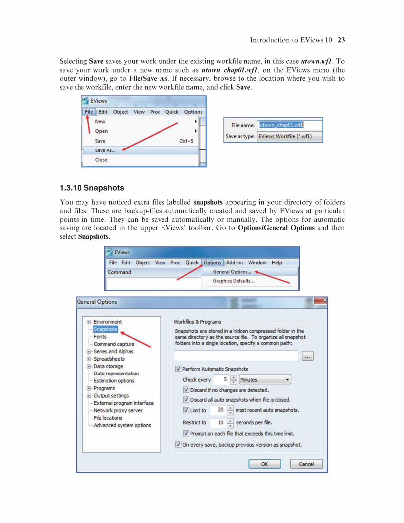
Selecting Save saves your work under the existing workfile name, in this case utown.wf1. To save your work under a new name such as utown_chap01.wf1, on the EViews menu (the outer window), go to File/Save As. If necessary, browse to the location where you wish to save the workfile, enter the new workfile name, and click Save.
1.3.10 Snapshots
You may have noticed extra files labelled snapshots appearing in your directory of folders and files. These are backup-files automatically created and saved by EViews at particular points in time. They can be saved automatically or manually. The options for automatic saving are located in the upper EViews’ toolbar. Go to Options/General Options and then select Snapshots.
24 Chapter 1
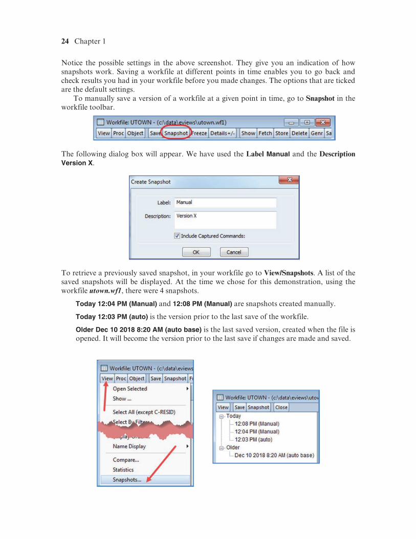
Notice the possible settings in the above screenshot. They give you an indication of how snapshots work. Saving a workfile at different points in time enables you to go back and check results you had in your workfile before you made changes. The options that are ticked are the default settings.
To manually save a version of a workfile at a given point in time, go to Snapshot in the workfile toolbar.
The following dialog box will appear. We have used the Label Manual and the Description Version X.
To retrieve a previously saved snapshot, in your workfile go to View/Snapshots. A list of the saved snapshots will be displayed. At the time we chose for this demonstration, using the workfile utown.wf1, there were 4 snapshots.
Today 12:04 PM (Manual) and 12:08 PM (Manual) are snapshots created manually.
Today 12:03 PM (auto) is the version prior to the last save of the workfile.
Older Dec 10 2018 8:20 AM (auto base) is the last saved version, created when the file is opened. It will become the version prior to the last save if changes are made and saved.
Introduction to EViews 10 25
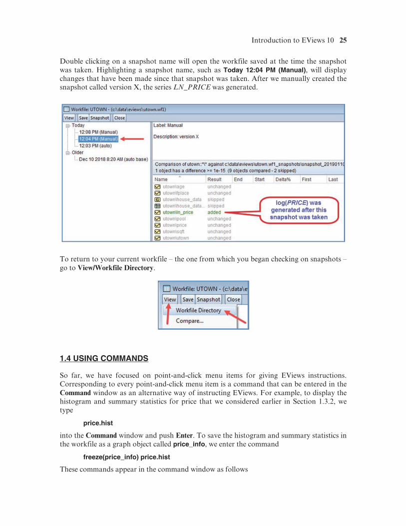
Double clicking on a snapshot name will open the workfile saved at the time the snapshot was taken. Highlighting a snapshot name, such as Today 12:04 PM (Manual), will display changes that have been made since that snapshot was taken. After we manually created the snapshot called version X, the series LN_PRICE was generated.
To return to your current workfile – the one from which you began checking on snapshots – go to View/Workfile Directory.
1.4 USING COMMANDS
So far, we have focused on point-and-click menu items for giving EViews instructions. Corresponding to every point-and-click menu item is a command that can be entered in the Command window as an alternative way of instructing EViews. For example, to display the histogram and summary statistics for price that we considered earlier in Section 1.3.2, we type
price.hist
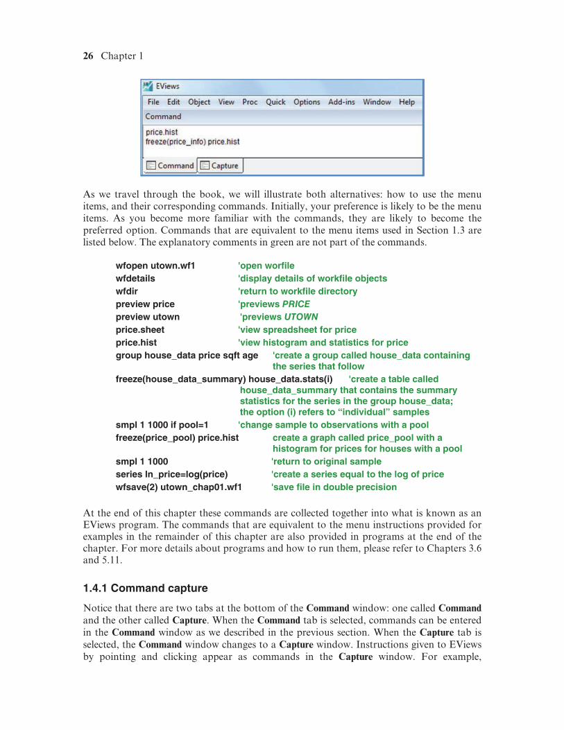
into the Command window and push Enter. To save the histogram and summary statistics in the workfile as a graph object called price_info, we enter the command
freeze(price_info) price.hist
These commands appear in the command window as follows
26 Chapter 1
As we travel through the book, we will illustrate both alternatives: how to use the menu items, and their corresponding commands. Initially, your preference is likely to be the menu items. As you become more familiar with the commands, they are likely to become the preferred option. Commands that are equivalent to the menu items used in Section 1.3 are listed below. The explanatory comments in green are not part of the commands.
wfopen utown.wf1 'open worfile wfdetails 'display details of workfile objects wfdir 'return to workfile directory preview price 'previews PRICE preview utown 'previews UTOWN price.sheet 'view spreadsheet for price price.hist 'view histogram and statistics for price group house_data price sqft age 'create a group called house_data containing
the series that follow freeze(house_data_summary) house_data.stats(i) 'create a table called
house_data_summary that contains the summary statistics for the series in the group house_data; the option (i) refers to “individual” samples
smpl 1 1000 if pool=1 'change sample to observations with a pool freeze(price_pool) price.hist create a graph called price_pool with a
histogram for prices for houses with a pool smpl 1 1000 'return to original sample series ln_price=log(price) 'create a series equal to the log of price wfsave(2) utown_chap01.wf1 'save file in double precision
At the end of this chapter these commands are collected together into what is known as an EViews program. The commands that are equivalent to the menu instructions provided for examples in the remainder of this chapter are also provided in programs at the end of the chapter. For more details about programs and how to run them, please refer to Chapters 3.6 and 5.11.
1.4.1 Command capture
Notice that there are two tabs at the bottom of the Command window: one called Command and the other called Capture. When the Command tab is selected, commands can be entered in the Command window as we described in the previous section. When the Capture tab is selected, the Command window changes to a Capture window. Instructions given to EViews by pointing and clicking appear as commands in the Capture window. For example,

Introduction to EViews 10 27
returning to the file utown_chap01.wf1, if we (1) create a group, (2) name that group grp, (3) View/Descriptive Statistics for grp, (4) Freeze those statistics into a table called grp_stats, and (5) close grp and grp_stats, the corresponding commands caught by the Capture window are in the screenshot on the right.
If you are wondering what the equivalent command is to a set of pointing-and-clicking steps, going to the Capture window can be a good way to find out. Commands in the Capture window can be copied and pasted into the Command window or a program.
1.4.2 Positioning the Command/Capture window
When EViews is first opened, the Command/Capture window is positioned horizontally at the top of the screen. Some users prefer a vertical window to the left of the screen. To change its position, hold the cursor down at the top of the command window.
Then, holding the cursor down, move the command window so that the cursor touches the arrow pointing left.
28 Chapter 1
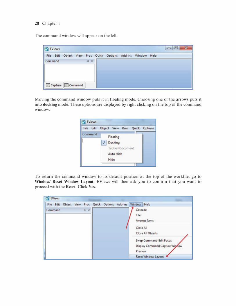
The command window will appear on the left.
Moving the command window puts it in floating mode. Choosing one of the arrows puts it into docking mode. These options are displayed by right clicking on the top of the command window.
To return the command window to its default position at the top of the workfile, go to Window/ Reset Window Layout. EViews will then ask you to confirm that you want to proceed with the Reset. Click Yes.
Introduction to EViews 10 29
1.5 A TIME-SERIES WORKFILE
In this section we explore further some of the capabilities of EViews, focusing particularly on creating graphs. We do so within the context of the workfile ozconfn.wf1 that contains quarterly time-series observations from quarter 1, 1975 to quarter 4, 2010 on the following Australian macroeconomic variables.
• CONS—real consumption expenditure, $billions
• CPI—consumer price index
• INC—real net national disposable income, $billions
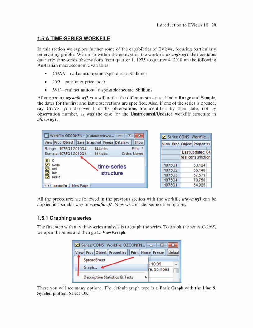
After opening ozconfn.wf1 you will notice the different structure. Under Range and Sample, the dates for the first and last observations are specified. Also, if one of the series is opened, say CONS, you discover that the observations are identified by their date, not by observation number, as was the case for the Unstructured/Undated workfile structure in utown.wf1.
All the procedures we followed in the previous section with the workfile utown.wf1 can be applied in a similar way to ozconfn.wf1. Now we consider some other options.
1.5.1 Graphing a series
The first step with any time-series analysis is to graph the series. To graph the series CONS, we open the series and then go to View/Graph.
There you will see many options. The default graph type is a Basic Graph with the Line & Symbol plotted. Select OK.
30 Chapter 1
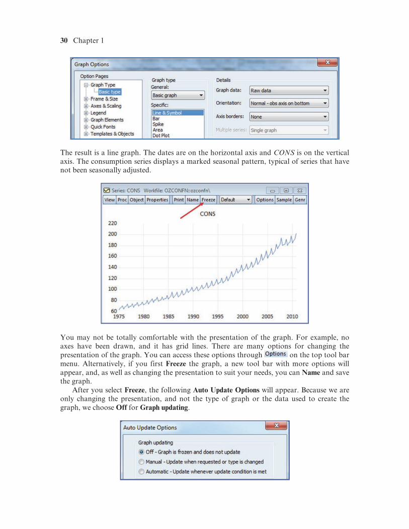
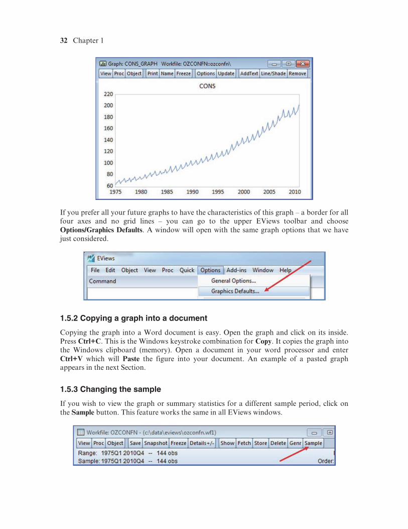
The result is a line graph. The dates are on the horizontal axis and CONS is on the vertical axis. The consumption series displays a marked seasonal pattern, typical of series that have not been seasonally adjusted.
You may not be totally comfortable with the presentation of the graph. For example, no axes have been drawn, and it has grid lines. There are many options for changing the presentation of the graph. You can access these options through on the top tool bar menu. Alternatively, if you first Freeze the graph, a new tool bar with more options will appear, and, as well as changing the presentation to suit your needs, you can Name and save the graph.
After you select Freeze, the following Auto Update Options will appear. Because we are only changing the presentation, and not the type of graph or the data used to create the graph, we choose Off for Graph updating.
Introduction to EViews 10 31
The graph will reappear, but notice the change in the top of the window. A Graph object has been created and the top toolbar has changed. Now, select Name and in the resulting dialog box, type in a name. We chose cons_graph. Then select Options.
There are a great many options that can be considered. When convenient, it is a good idea to explore these options, and experiment with them until the presentation of a graph is to your liking. At present, we will take steps to create axes and eliminate the grid lines. Go to Frame &Size/Color & Border/Frame border/Axes and choose the desired axes. We have chosen to insert axes on all four sides of the graph. Then click Apply that you will find at the bottom of the window.
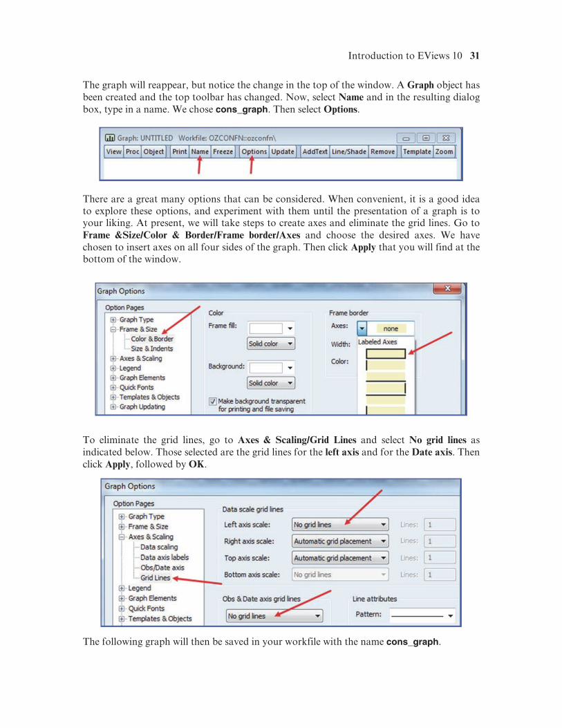
To eliminate the grid lines, go to Axes & Scaling/Grid Lines and select No grid lines as indicated below. Those selected are the grid lines for the left axis and for the Date axis. Then click Apply, followed by OK.
The following graph will then be saved in your workfile with the name cons_graph.
32 Chapter 1
If you prefer all your future graphs to have the characteristics of this graph – a border for all four axes and no grid lines – you can go to the upper EViews toolbar and choose Options/Graphics Defaults. A window will open with the same graph options that we have just considered.
1.5.2 Copying a graph into a document
Copying the graph into a Word document is easy. Open the graph and click on its inside. Press Ctrl+C. This is the Windows keystroke combination for Copy. It copies the graph into the Windows clipboard (memory). Open a document in your word processor and enter Ctrl+V which will Paste the figure into your document. An example of a pasted graph appears in the next Section.
1.5.3 Changing the sample
If you wish to view the graph or summary statistics for a different sample period, click on the Sample button. This feature works the same in all EViews windows.
Introduction to EViews 10 33
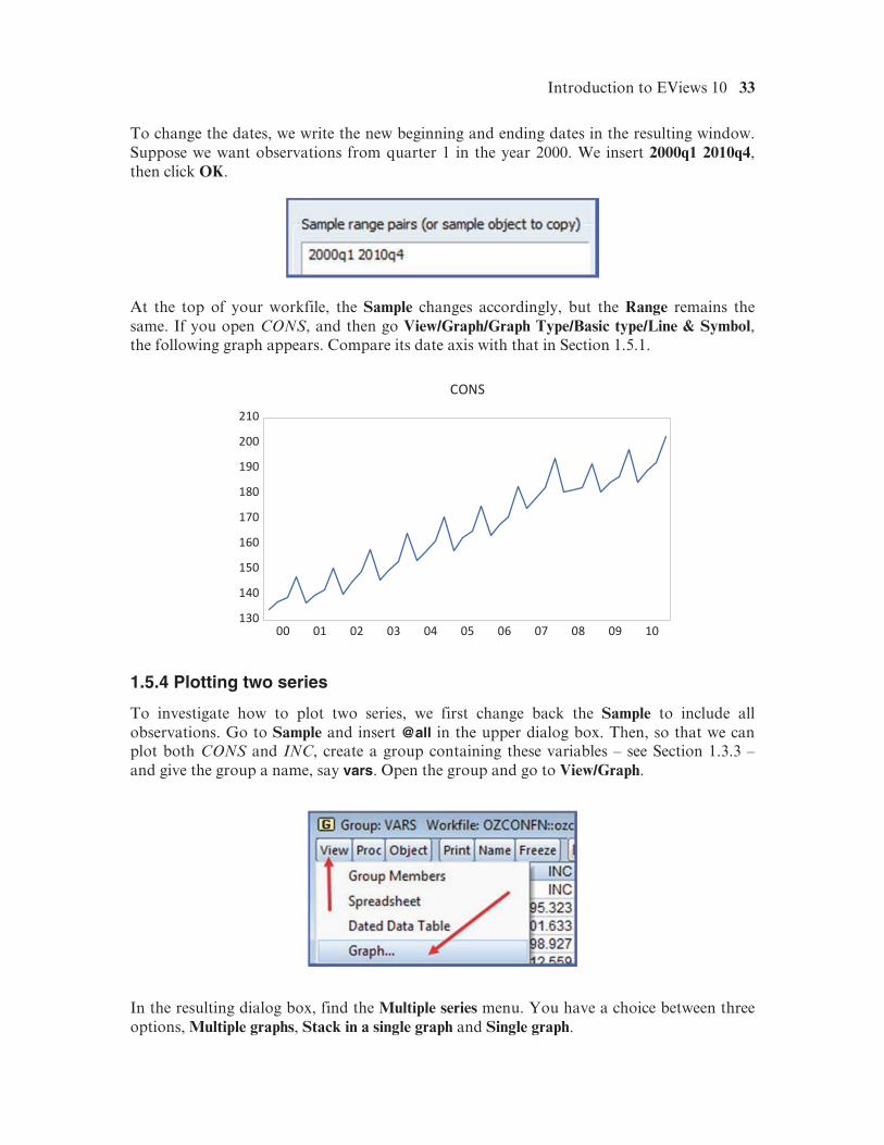
To change the dates, we write the new beginning and ending dates in the resulting window. Suppose we want observations from quarter 1 in the year 2000. We insert 2000q1 2010q4, then click OK.
At the top of your workfile, the Sample changes accordingly, but the Range remains the same. If you open CONS, and then go View/Graph/Graph Type/Basic type/Line & Symbol, the following graph appears. Compare its date axis with that in Section 1.5.1.
1.5.4 Plotting two series
To investigate how to plot two series, we first change back the Sample to include all observations. Go to Sample and insert @all in the upper dialog box. Then, so that we can plot both CONS and INC, create a group containing these variables – see Section 1.3.3 – and give the group a name, say vars. Open the group and go to View/Graph.
In the resulting dialog box, find the Multiple series menu. You have a choice between three options, Multiple graphs, Stack in a single graph and Single graph.
34 Chapter 1
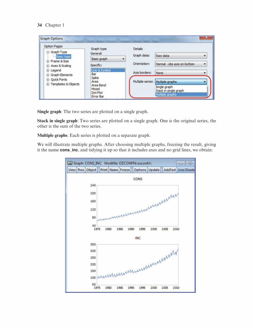
Single graph: The two series are plotted on a single graph.
Stack in single graph: Two series are plotted on a single graph. One is the original series, the other is the sum of the two series.
Multiple graphs: Each series is plotted on a separate graph.
We will illustrate multiple graphs. After choosing multiple graphs, freezing the result, giving it the name cons_inc, and tidying it up so that it includes axes and no grid lines, we obtain:
Introduction to EViews 10 35
1.5.5 A scatter diagram
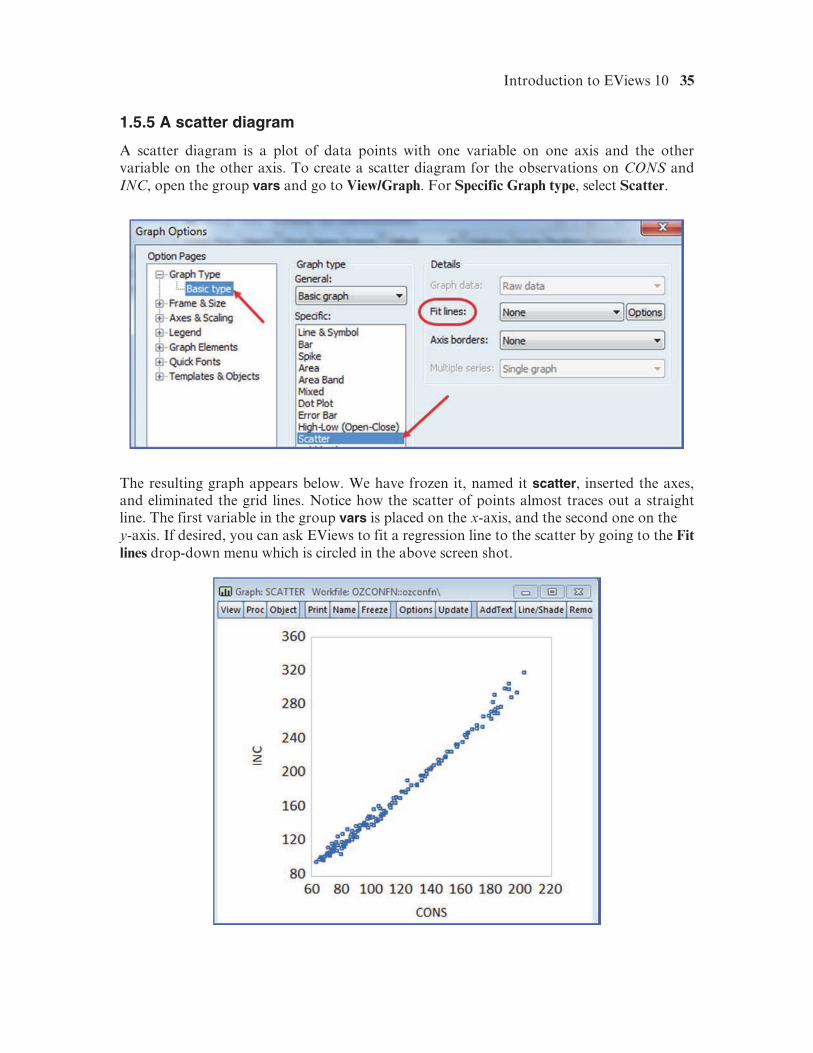
A scatter diagram is a plot of data points with one variable on one axis and the other variable on the other axis. To create a scatter diagram for the observations on CONS and INC, open the group vars and go to View/Graph. For Specific Graph type, select Scatter.
The resulting graph appears below. We have frozen it, named it scatter, inserted the axes, and eliminated the grid lines. Notice how the scatter of points almost traces out a straight line. The first variable in the group vars is placed on the x-axis, and the second one on the y-axis. If desired, you can ask EViews to fit a regression line to the scatter by going to the Fit lines drop-down menu which is circled in the above screen shot.
36 Chapter 1
1.6 USING THE QUICK MENU
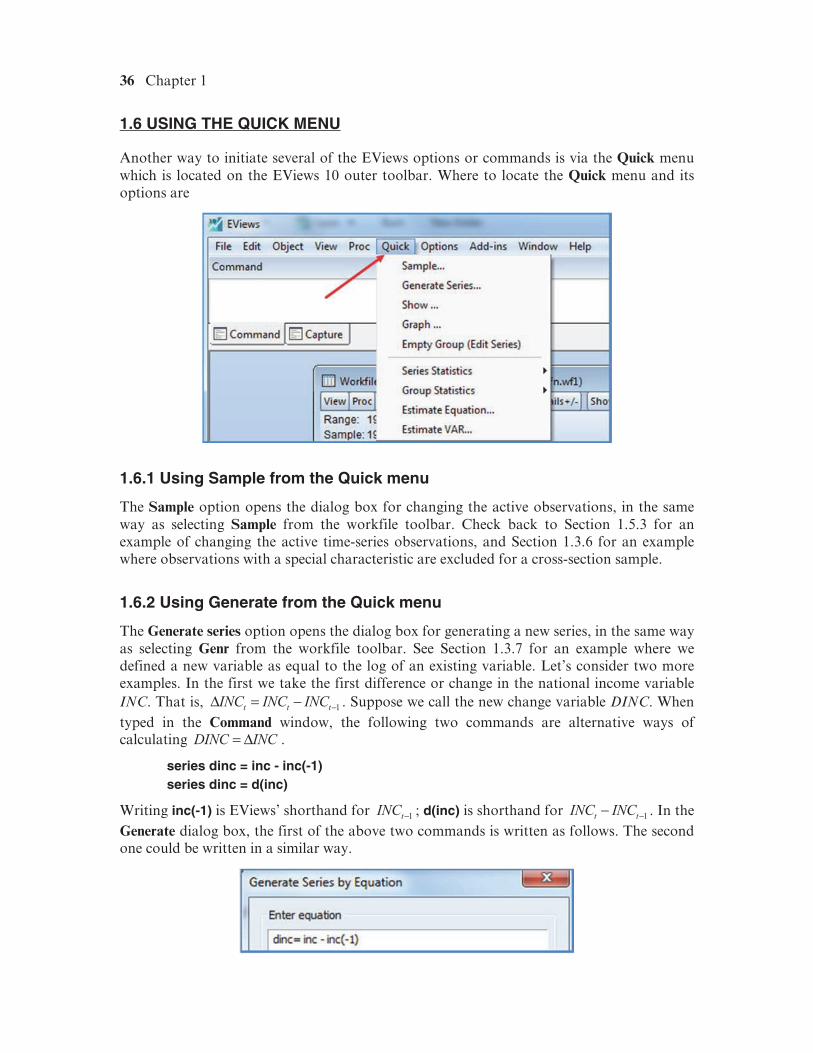
Another way to initiate several of the EViews options or commands is via the Quick menu which is located on the EViews 10 outer toolbar. Where to locate the Quick menu and its options are
1.6.1 Using Sample from the Quick menu
The Sample option opens the dialog box for changing the active observations, in the same way as selecting Sample from the workfile toolbar. Check back to Section 1.5.3 for an example of changing the active time-series observations, and Section 1.3.6 for an example where observations with a special characteristic are excluded for a cross-section sample.
1.6.2 Using Generate from the Quick menu
The Generate series option opens the dialog box for generating a new series, in the same way as selecting Genr from the workfile toolbar. See Section 1.3.7 for an example where we defined a new variable as equal to the log of an existing variable. Let’s consider two more examples. In the first we take the first difference or change in the national income variable INC. That is, −Δ = − . Suppose we call the new change variable DINC. When typed in the Command window, the following two commands are alternative ways of calculating = Δ .
series dinc = inc - inc(-1) series dinc = d(inc)
Writing inc(-1) is EViews’ shorthand for − ; d(inc) is shorthand for −− . In the Generate dialog box, the first of the above two commands is written as follows. The second one could be written in a similar way.
Introduction to EViews 10 37
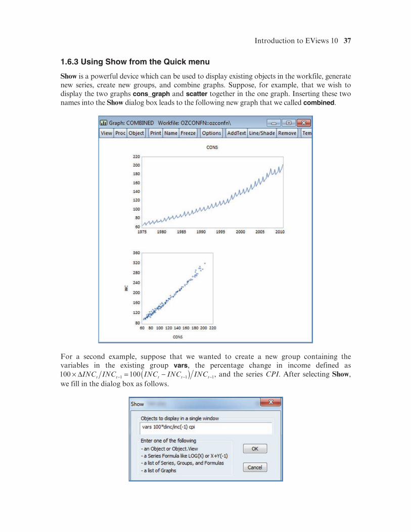
1.6.3 Using Show from the Quick menu
Show is a powerful device which can be used to display existing objects in the workfile, generate new series, create new groups, and combine graphs. Suppose, for example, that we wish to display the two graphs cons_graph and scatter together in the one graph. Inserting these two names into the Show dialog box leads to the following new graph that we called combined.
For a second example, suppose that we wanted to create a new group containing the variables in the existing group vars, the percentage change in income defined as
( )− − −× Δ = −1 1 1100 100t t t t tINC INC INC INC INC , and the series CPI. After selecting Show, we fill in the dialog box as follows.
38 Chapter 1
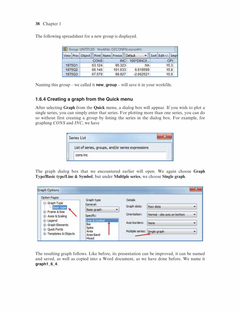
The following spreadsheet for a new group is displayed.
Naming this group – we called it new_group – will save it in your workfile.
1.6.4 Creating a graph from the Quick menu
After selecting Graph from the Quick menu, a dialog box will appear. If you wish to plot a single series, you can simply enter that series. For plotting more than one series, you can do so without first creating a group by listing the series in the dialog box. For example, for graphing CONS and INC, we have
The graph dialog box that we encountered earlier will open. We again choose Graph Type/Basic type/Line & Symbol, but under Multiple series, we choose Single graph.
The resulting graph follows. Like before, its presentation can be improved, it can be named and saved, as well as copied into a Word document, as we have done before. We name it graph1_6_4.
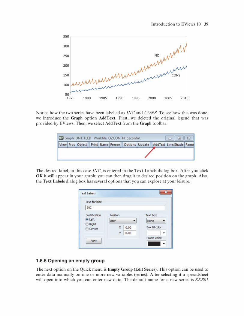
Introduction to EViews 10 39
Notice how the two series have been labelled as INC and CONS. To see how this was done, we introduce the Graph option AddText. First, we deleted the original legend that was provided by EViews. Then, we select AddText from the Graph toolbar.
The desired label, in this case INC, is entered in the Text Labels dialog box. After you click OK it will appear in your graph; you can then drag it to desired position on the graph. Also, the Text Labels dialog box has several options that you can explore at your leisure.
1.6.5 Opening an empty group
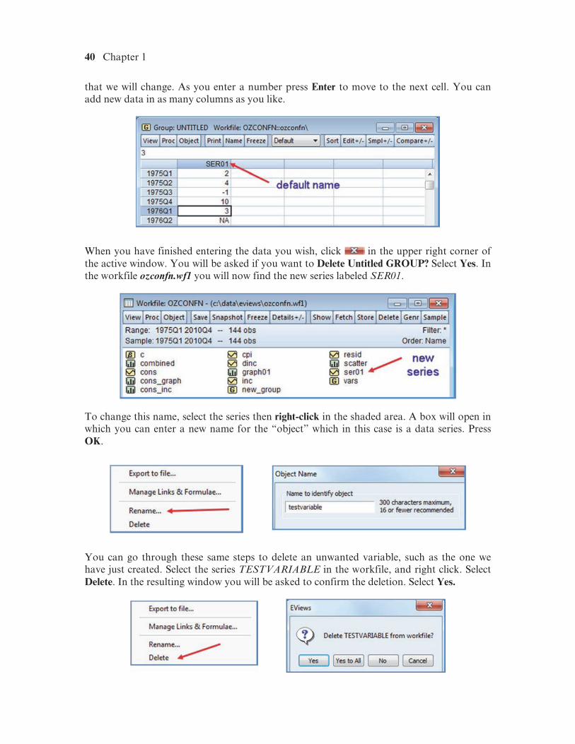
The next option on the Quick menu is Empty Group (Edit Series). This option can be used to enter data manually on one or more new variables (series). After selecting it a spreadsheet will open into which you can enter new data. The default name for a new series is SER01
40 Chapter 1
that we will change. As you enter a number press Enter to move to the next cell. You can add new data in as many columns as you like.
When you have finished entering the data you wish, click in the upper right corner of the active window. You will be asked if you want to Delete Untitled GROUP? Select Yes. In the workfile ozconfn.wf1 you will now find the new series labeled SER01.
To change this name, select the series then right-click in the shaded area. A box will open in which you can enter a new name for the “object” which in this case is a data series. Press OK.
You can go through these same steps to delete an unwanted variable, such as the one we have just created. Select the series TESTVARIABLE in the workfile, and right click. Select Delete. In the resulting window you will be asked to confirm the deletion. Select Yes.
Introduction to EViews 10 41
The commands for renaming and deleting are
rename ser01 testvariable delete testvariable
More than one series or objects can be selected for deletion by selecting one, and then holding down the Ctrl-key while selecting others. To delete all these selected objects right-click in the blue area, and repeat the steps above. Alternatively, after selecting the objects marked for deletion, click on Delete from the workfile toolbar.
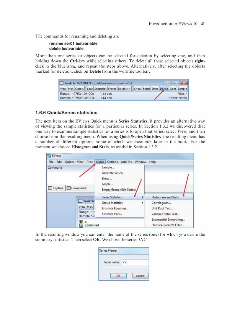
1.6.6 Quick/Series statistics
The next item on the EViews Quick menu is Series Statistics; it provides an alternative way of viewing the sample statistics for a particular series. In Section 1.3.2 we discovered that one way to examine sample statistics for a series is to open that series, select View, and then choose from the resulting menu. When using Quick/Series Statistics, the resulting menu has a number of different options, some of which we encounter later in the book. For the moment we choose Histogram and Stats, as we did in Section 1.3.2.
In the resulting window you can enter the name of the series (one) for which you desire the summary statistics. Then select OK. We chose the series INC.
42 Chapter 1
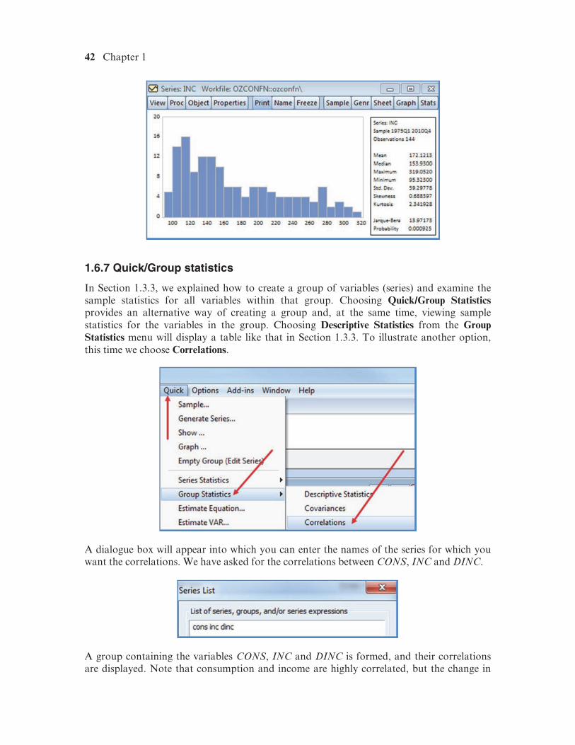
1.6.7 Quick/Group statistics
In Section 1.3.3, we explained how to create a group of variables (series) and examine the sample statistics for all variables within that group. Choosing Quick/Group Statistics provides an alternative way of creating a group and, at the same time, viewing sample statistics for the variables in the group. Choosing Descriptive Statistics from the Group Statistics menu will display a table like that in Section 1.3.3. To illustrate another option, this time we choose Correlations.
A dialogue box will appear into which you can enter the names of the series for which you want the correlations. We have asked for the correlations between CONS, INC and DINC.
A group containing the variables CONS, INC and DINC is formed, and their correlations are displayed. Note that consumption and income are highly correlated, but the change in
Introduction to EViews 10 43
income is not highly correlated with consumption, nor income. If you wish to retain the group, you can select Name, and give the group a name. If you wish to keep the correlations in your workfile, select Freeze, and give the resulting table a name, say cor1_6_7.
It is convenient at this point to save the workfile; using Save As (see Section 1.3.9), we call the saved file ozconfn_chap01.wf1.
1.6.8 Other Quick menu items
The remaining items on the Quick menu are Estimate Equation and Estimate VAR. These items will be introduced in Chapters 2 and 13, respectively.
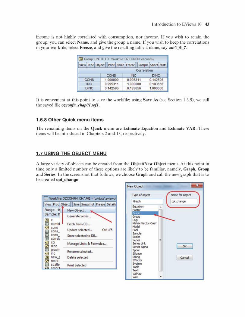
1.7 USING THE OBJECT MENU
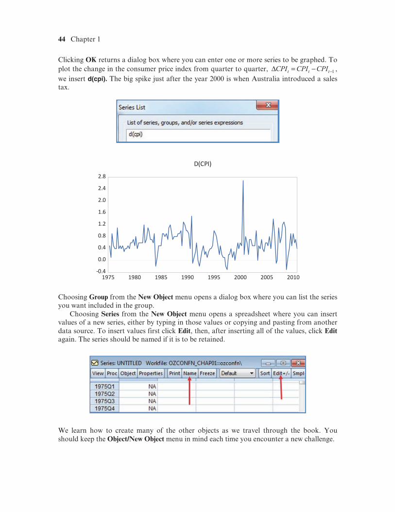
A large variety of objects can be created from the Object/New Object menu. At this point in time only a limited number of these options are likely to be familiar, namely, Graph, Group and Series. In the screenshot that follows, we choose Graph and call the new graph that is to be created cpi_change.
44 Chapter 1
Clicking OK returns a dialog box where you can enter one or more series to be graphed. To plot the change in the consumer price index from quarter to quarter, −Δ = − , we insert d(cpi). The big spike just after the year 2000 is when Australia introduced a sales tax.
Choosing Group from the New Object menu opens a dialog box where you can list the series you want included in the group.
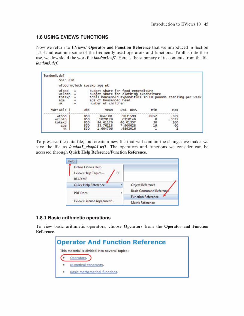
Choosing Series from the New Object menu opens a spreadsheet where you can insert values of a new series, either by typing in those values or copying and pasting from another data source. To insert values first click Edit, then, after inserting all of the values, click Edit again. The series should be named if it is to be retained.
We learn how to create many of the other objects as we travel through the book. You should keep the Object/New Object menu in mind each time you encounter a new challenge.
Introduction to EViews 10 45
1.8 USING EVIEWS FUNCTIONS
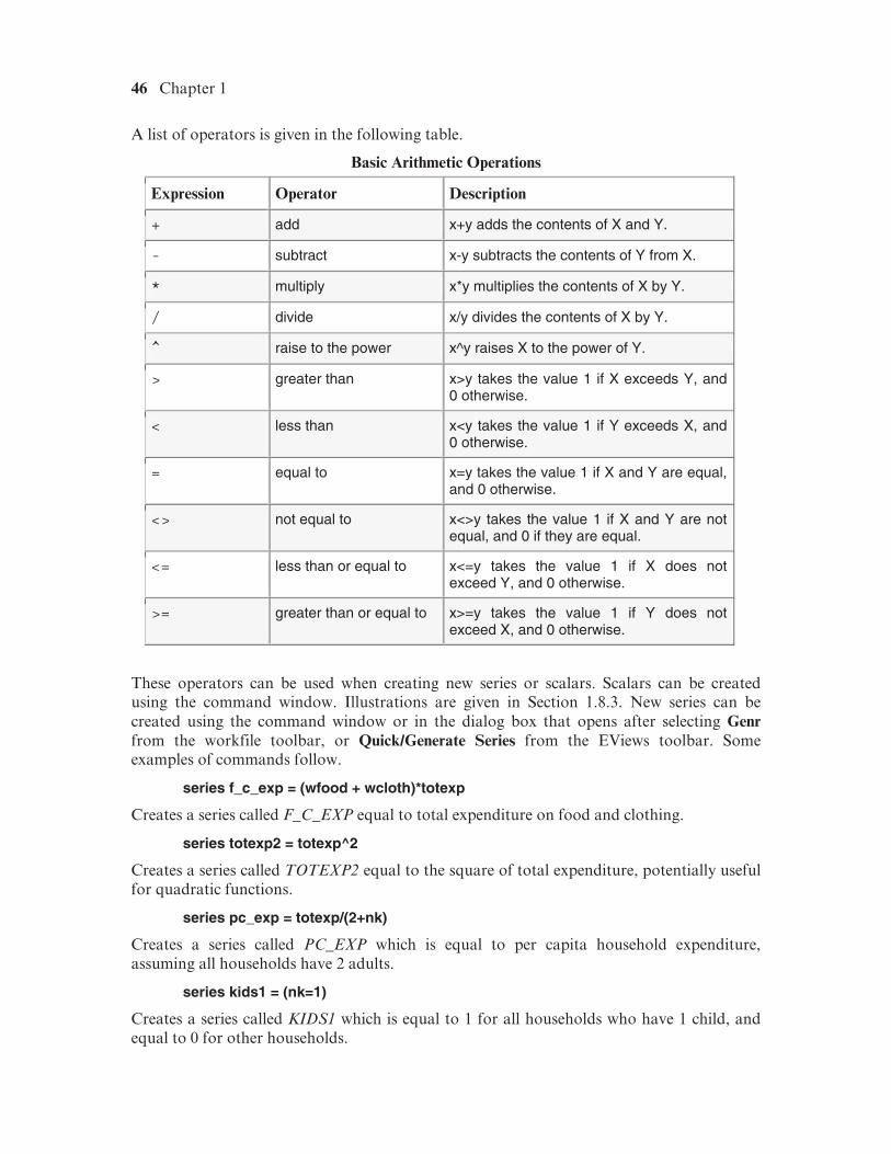
Now we return to EViews’ Operator and Function Reference that we introduced in Section 1.2.3 and examine some of the frequently-used operators and functions. To illustrate their use, we download the workfile london5.wf1. Here is the summary of its contents from the file london5.def.
To preserve the data file, and create a new file that will contain the changes we make, we save the file as london5_chap01.wf1. The operators and functions we consider can be accessed through Quick Help Reference/Function Reference.
1.8.1 Basic arithmetic operations
To view basic arithmetic operators, choose Operators from the Operator and Function Reference.
46 Chapter 1
A list of operators is given in the following table.
Basic Arithmetic Operations
Expression Operator Description
+ add x+y adds the contents of X and Y.
- subtract x-y subtracts the contents of Y from X.
* multiply x*y multiplies the contents of X by Y.
/ divide x/y divides the contents of X by Y.
^ raise to the power x^y raises X to the power of Y.
> greater than x>y takes the value 1 if X exceeds Y, and 0 otherwise.
< less than x<y takes the value 1 if Y exceeds X, and 0 otherwise.
= equal to x=y takes the value 1 if X and Y are equal, and 0 otherwise.
<> not equal to x<>y takes the value 1 if X and Y are not equal, and 0 if they are equal.
<= less than or equal to x<=y takes the value 1 if X does not exceed Y, and 0 otherwise.
>= greater than or equal to x>=y takes the value 1 if Y does not exceed X, and 0 otherwise.
These operators can be used when creating new series or scalars. Scalars can be created using the command window. Illustrations are given in Section 1.8.3. New series can be created using the command window or in the dialog box that opens after selecting Genr from the workfile toolbar, or Quick/Generate Series from the EViews toolbar. Some examples of commands follow.
series f_c_exp = (wfood + wcloth)*totexp
Creates a series called F_C_EXP equal to total expenditure on food and clothing.
series totexp2 = totexp^2
Creates a series called TOTEXP2 equal to the square of total expenditure, potentially useful for quadratic functions.
series pc_exp = totexp/(2+nk)
Creates a series called PC_EXP which is equal to per capita household expenditure, assuming all households have 2 adults.
series kids1 = (nk=1)
Creates a series called KIDS1 which is equal to 1 for all households who have 1 child, and equal to 0 for other households.
Introduction to EViews 10 47
After entering these commands, the command window will appear as:
If the Genr dialog box is used as an alternative, “series” is omitted. For example, for F_C_EXP:
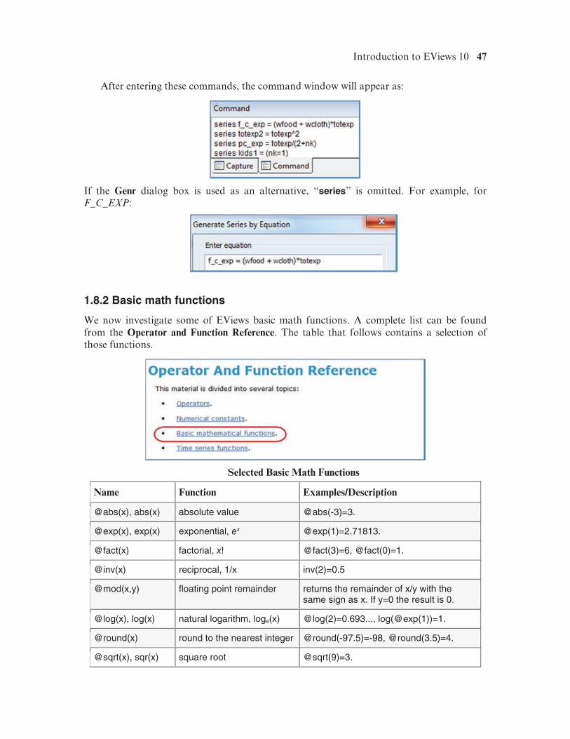
1.8.2 Basic math functions
We now investigate some of EViews basic math functions. A complete list can be found from the Operator and Function Reference. The table that follows contains a selection of those functions.
Selected Basic Math Functions
Name Function Examples/Description
@abs(x), abs(x) absolute value @abs(-3)=3.
@exp(x), exp(x) exponential, ex @exp(1)=2.71813.
@fact(x) factorial, x! @fact(3)=6, @fact(0)=1.
@inv(x) reciprocal, 1/x inv(2)=0.5
@mod(x,y) floating point remainder returns the remainder of x/y with the same sign as x. If y=0 the result is 0.
@log(x), log(x) natural logarithm, loge(x) @log(2)=0.693..., log(@exp(1))=1.
@round(x) round to the nearest integer @round(-97.5)=-98, @round(3.5)=4.
@sqrt(x), sqr(x) square root @sqrt(9)=3.
48 Chapter 1
Note how the functions begin with the “@” symbol. Common ones like the absolute value (abs), the exponential function (exp), the natural logarithm (log) and the square root (sqr) can be used with or without the @ sign.
The command to create a series LN_TOTEXP that is the natural logarithm of total expenditure is
series ln_totexp = log(totexp)
Notice that the series of proportions WFOOD and WCLOTH are reported to 4 decimal places. Suppose that we want to round off WFOOD to 2 decimal places and store the result as WFOOD2. We can use the command
series wfood2 = @round(wfood*100)/100
These commands can also be executed by typing them in the Genr dialog box, with series omitted.
1.8.3 Descriptive statistics functions
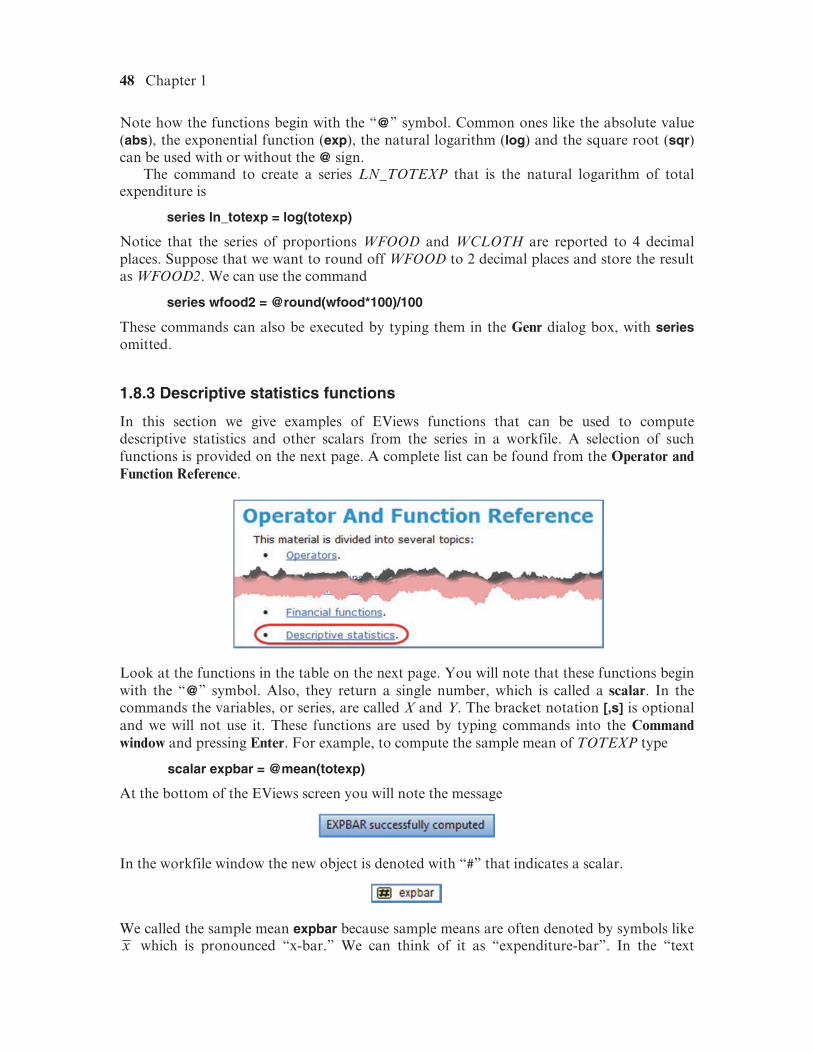
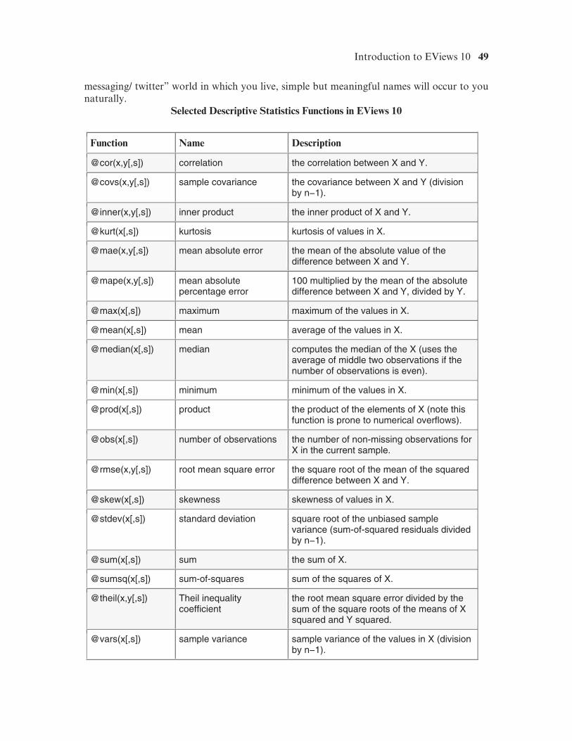
In this section we give examples of EViews functions that can be used to compute descriptive statistics and other scalars from the series in a workfile. A selection of such functions is provided on the next page. A complete list can be found from the Operator and Function Reference.
Look at the functions in the table on the next page. You will note that these functions begin with the “@” symbol. Also, they return a single number, which is called a scalar. In the commands the variables, or series, are called X and Y. The bracket notation [,s] is optional and we will not use it. These functions are used by typing commands into the Command window and pressing Enter. For example, to compute the sample mean of TOTEXP type
scalar expbar = @mean(totexp)
At the bottom of the EViews screen you will note the message
In the workfile window the new object is denoted with “#” that indicates a scalar.
We called the sample mean expbar because sample means are often denoted by symbols like which is pronounced “x-bar.” We can think of it as “expenditure-bar”. In the “text
Introduction to EViews 10 49
messaging/ twitter” world in which you live, simple but meaningful names will occur to you naturally.
Selected Descriptive Statistics Functions in EViews 10
Function Name Description
@cor(x,y[,s]) correlation the correlation between X and Y.
@covs(x,y[,s]) sample covariance the covariance between X and Y (division by n−1).
@inner(x,y[,s]) inner product the inner product of X and Y.
@kurt(x[,s]) kurtosis kurtosis of values in X.
@mae(x,y[,s]) mean absolute error the mean of the absolute value of the difference between X and Y.
@mape(x,y[,s]) mean absolute percentage error
100 multiplied by the mean of the absolute difference between X and Y, divided by Y.
@max(x[,s]) maximum maximum of the values in X.
@mean(x[,s]) mean average of the values in X.
@median(x[,s]) median computes the median of the X (uses the average of middle two observations if the number of observations is even).
@min(x[,s]) minimum minimum of the values in X.
@prod(x[,s]) product the product of the elements of X (note this function is prone to numerical overflows).
@obs(x[,s]) number of observations the number of non-missing observations for X in the current sample.
@rmse(x,y[,s]) root mean square error the square root of the mean of the squared difference between X and Y.
@skew(x[,s]) skewness skewness of values in X.
@stdev(x[,s]) standard deviation square root of the unbiased sample variance (sum-of-squared residuals divided by n−1).
@sum(x[,s]) sum the sum of X.
@sumsq(x[,s]) sum-of-squares sum of the squares of X.
@theil(x,y[,s]) Theil inequality coefficient
the root mean square error divided by the sum of the square roots of the means of X squared and Y squared.
@vars(x[,s]) sample variance sample variance of the values in X (division by n−1).
50 Chapter 1
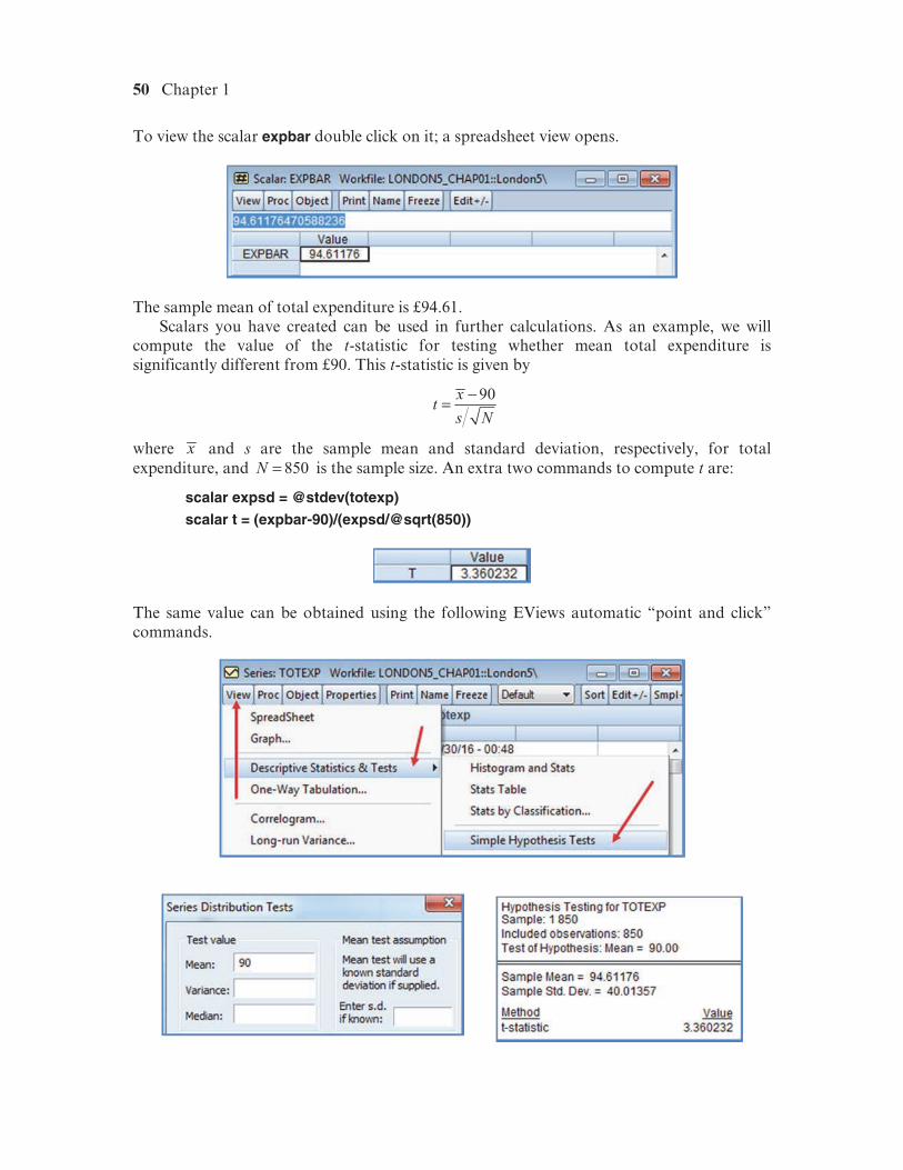
To view the scalar expbar double click on it; a spreadsheet view opens.
The sample mean of total expenditure is £94.61. Scalars you have created can be used in further calculations. As an example, we will
compute the value of the t-statistic for testing whether mean total expenditure is significantly different from £90. This t-statistic is given by
−=
where and s are the sample mean and standard deviation, respectively, for total expenditure, and = is the sample size. An extra two commands to compute t are:
scalar expsd = @stdev(totexp)
scalar t = (expbar-90)/(expsd/@sqrt(850))
The same value can be obtained using the following EViews automatic “point and click” commands.
Introduction to EViews 10 51
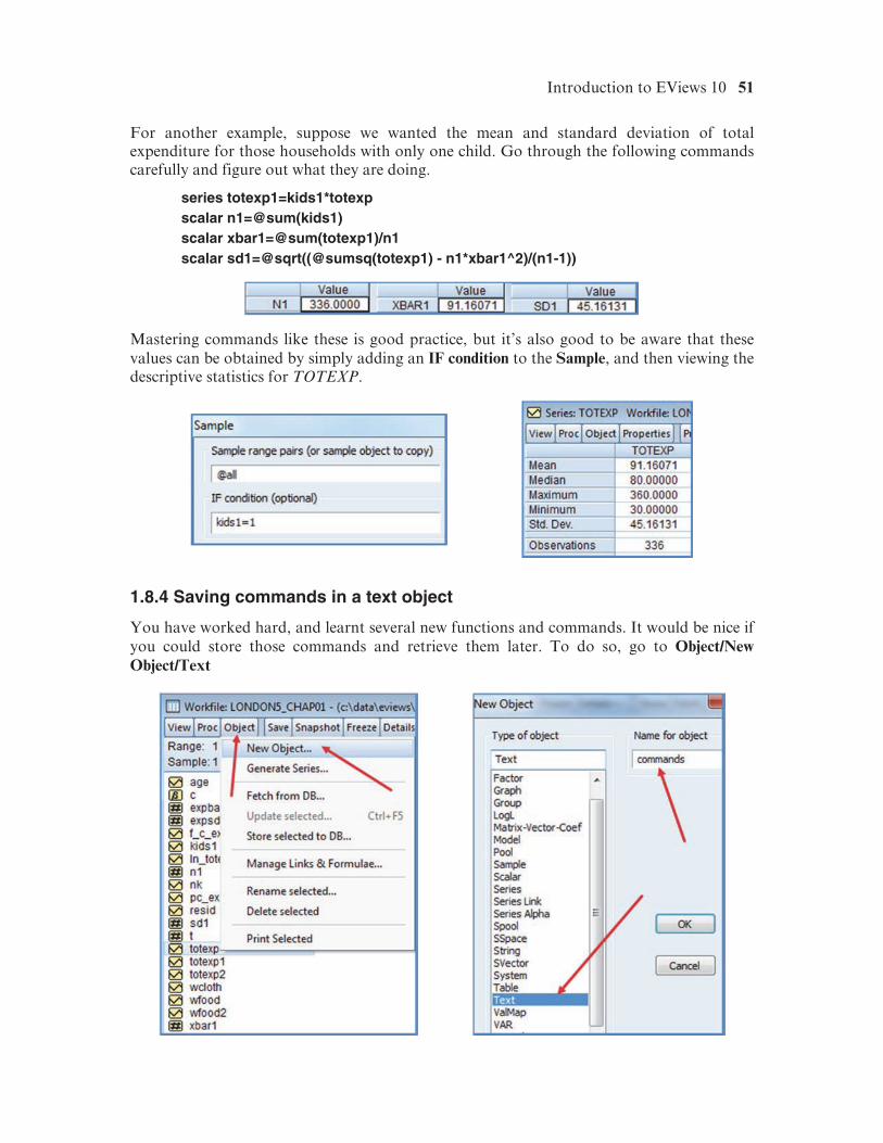
For another example, suppose we wanted the mean and standard deviation of total expenditure for those households with only one child. Go through the following commands carefully and figure out what they are doing.
series totexp1=kids1*totexp scalar n1=@sum(kids1) scalar xbar1=@sum(totexp1)/n1 scalar sd1=@sqrt((@sumsq(totexp1) - n1*xbar1^2)/(n1-1))
Mastering commands like these is good practice, but it’s also good to be aware that these values can be obtained by simply adding an IF condition to the Sample, and then viewing the descriptive statistics for TOTEXP.
1.8.4 Saving commands in a text object
You have worked hard, and learnt several new functions and commands. It would be nice if you could store those commands and retrieve them later. To do so, go to Object/New Object/Text
52 Chapter 1
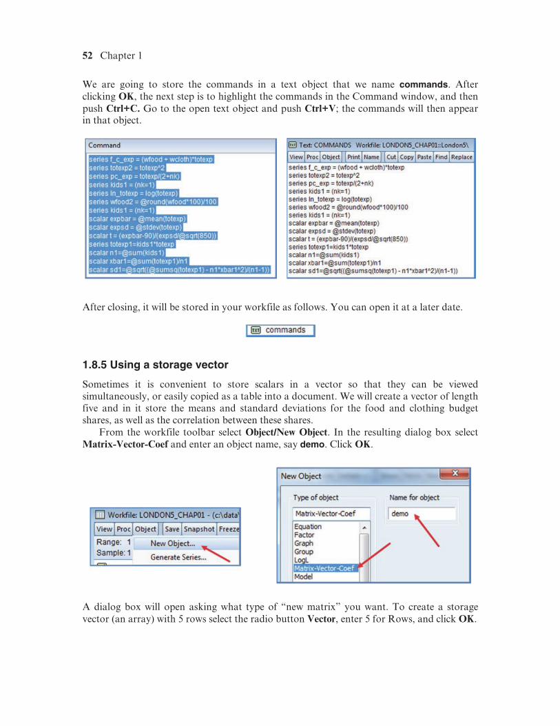
We are going to store the commands in a text object that we name commands. After clicking OK, the next step is to highlight the commands in the Command window, and then push Ctrl+C. Go to the open text object and push Ctrl+V; the commands will then appear in that object.
After closing, it will be stored in your workfile as follows. You can open it at a later date.
1.8.5 Using a storage vector
Sometimes it is convenient to store scalars in a vector so that they can be viewed simultaneously, or easily copied as a table into a document. We will create a vector of length five and in it store the means and standard deviations for the food and clothing budget shares, as well as the correlation between these shares.
From the workfile toolbar select Object/New Object. In the resulting dialog box select Matrix-Vector-Coef and enter an object name, say demo. Click OK.
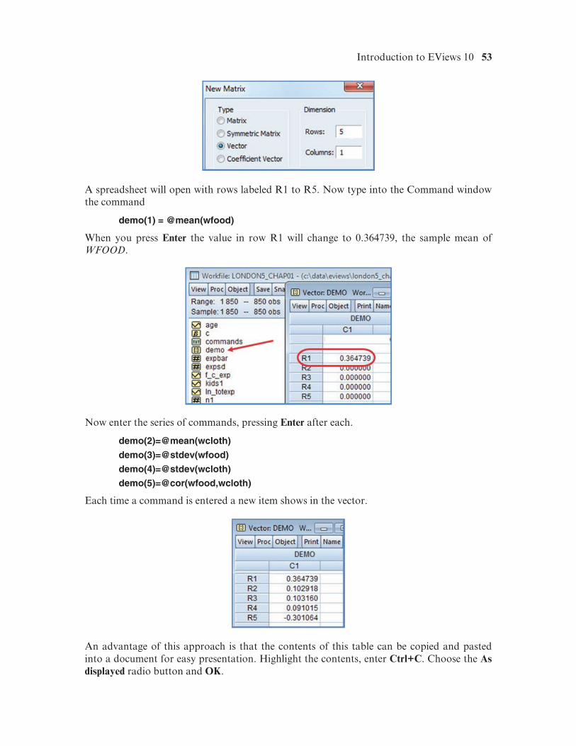
A dialog box will open asking what type of “new matrix” you want. To create a storage vector (an array) with 5 rows select the radio button Vector, enter 5 for Rows, and click OK.
Introduction to EViews 10 53
A spreadsheet will open with rows labeled R1 to R5. Now type into the Command window the command
demo(1) = @mean(wfood)
When you press Enter the value in row R1 will change to 0.364739, the sample mean of WFOOD.
Now enter the series of commands, pressing Enter after each.
demo(2)=@mean(wcloth)
demo(3)=@stdev(wfood)
demo(4)=@stdev(wcloth)
demo(5)=@cor(wfood,wcloth)
Each time a command is entered a new item shows in the vector.
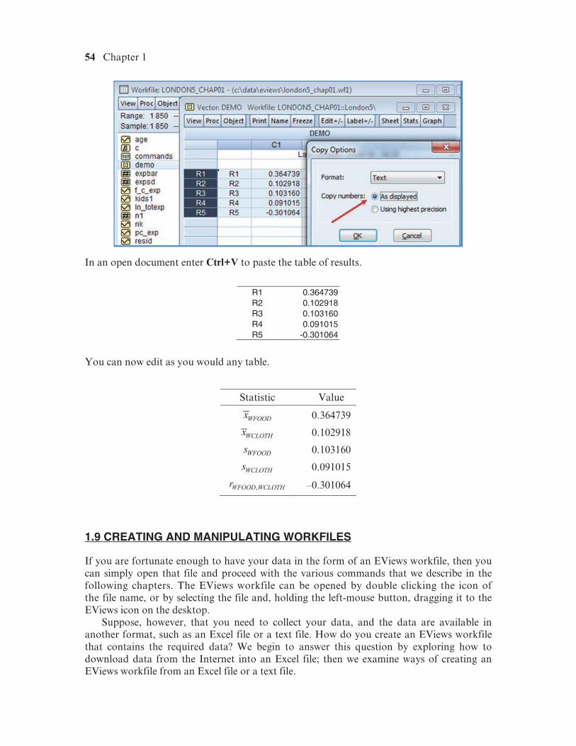
An advantage of this approach is that the contents of this table can be copied and pasted into a document for easy presentation. Highlight the contents, enter Ctrl+C. Choose the As displayed radio button and OK.
54 Chapter 1
In an open document enter Ctrl+V to paste the table of results.
R1 0.364739R2 0.102918R3 0.103160R4 0.091015R5 -0.301064
You can now edit as you would any table.
Statistic Value
0.364739
0.102918
0.103160
0.091015
–0.301064
1.9 CREATING AND MANIPULATING WORKFILES
If you are fortunate enough to have your data in the form of an EViews workfile, then you can simply open that file and proceed with the various commands that we describe in the following chapters. The EViews workfile can be opened by double clicking the icon of the file name, or by selecting the file and, holding the left-mouse button, dragging it to the EViews icon on the desktop.
Suppose, however, that you need to collect your data, and the data are available in another format, such as an Excel file or a text file. How do you create an EViews workfile that contains the required data? We begin to answer this question by exploring how to download data from the Internet into an Excel file; then we examine ways of creating an EViews workfile from an Excel file or a text file.
Introduction to EViews 10 55
1.9.1 Obtaining data from the Internet
Getting data for economic research is much easier today than it was years ago. Before the Internet, hours would be spent in libraries, looking for and copying data by hand. Now we have access to rich data sources which are a few clicks away.
Suppose you are interested in analyzing the GDP of the United States. As suggested in Chapter 1 of POE5, the website Resources for Economists contains a wide variety of data, and in particular the macro data we seek. Websites are continually updated and improved. We shall guide you through an example, but be prepared for differences from what we show here.
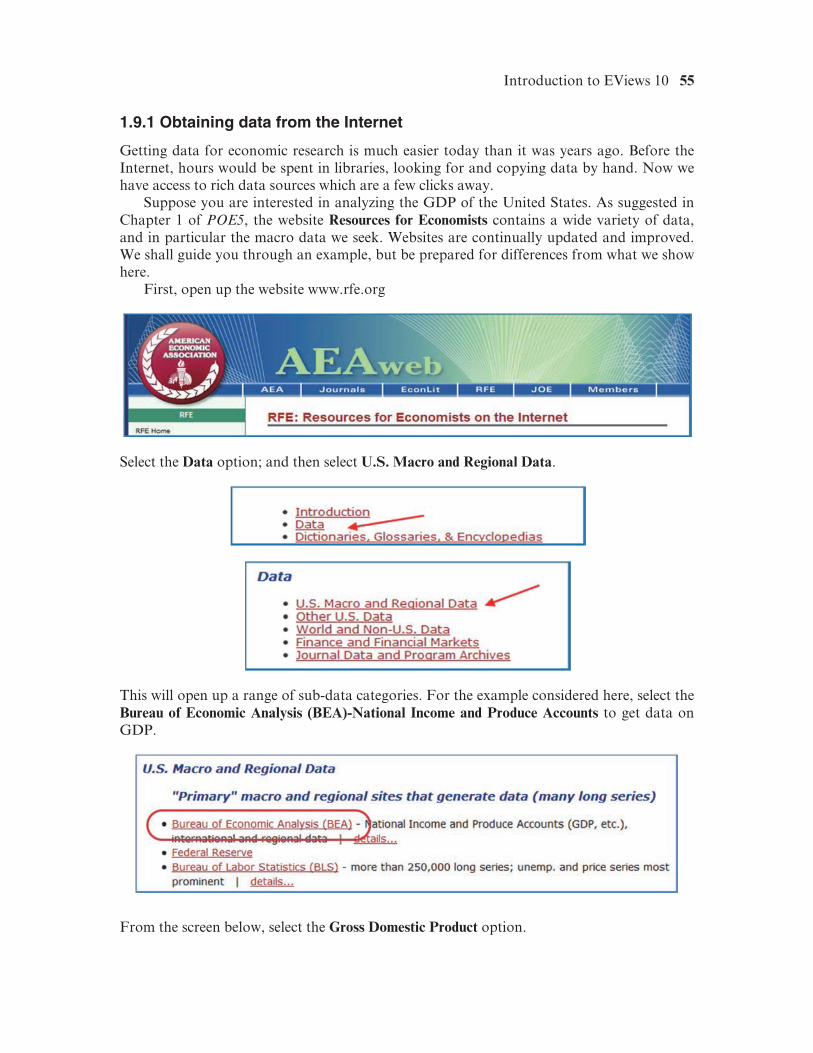
First, open up the website www.rfe.org
Select the Data option; and then select U.S. Macro and Regional Data.
This will open up a range of sub-data categories. For the example considered here, select the Bureau of Economic Analysis (BEA)-National Income and Produce Accounts to get data on GDP.
From the screen below, select the Gross Domestic Product option.
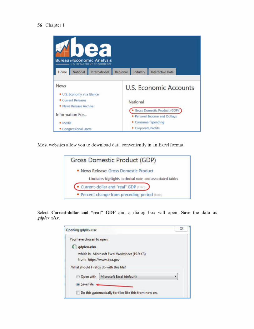
56 Chapter 1
Most websites allow you to download data conveniently in an Excel format.
Select Current-dollar and “real” GDP and a dialog box will open. Save the data as gdplev.xlsx.
Introduction to EViews 10 57
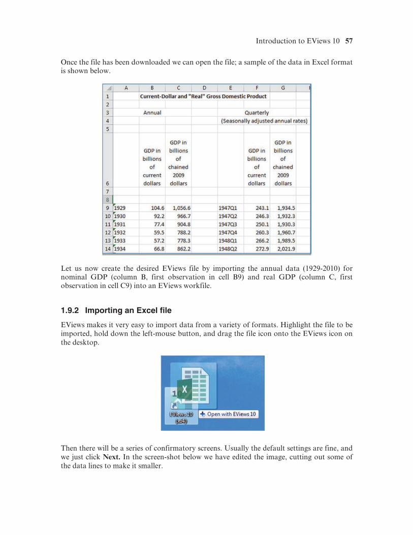
Once the file has been downloaded we can open the file; a sample of the data in Excel format is shown below.
Let us now create the desired EViews file by importing the annual data (1929-2010) for nominal GDP (column B, first observation in cell B9) and real GDP (column C, first observation in cell C9) into an EViews workfile.
1.9.2 Importing an Excel file
EViews makes it very easy to import data from a variety of formats. Highlight the file to be imported, hold down the left-mouse button, and drag the file icon onto the EViews icon on the desktop.
Then there will be a series of confirmatory screens. Usually the default settings are fine, and we just click Next. In the screen-shot below we have edited the image, cutting out some of the data lines to make it smaller.
58 Chapter 1
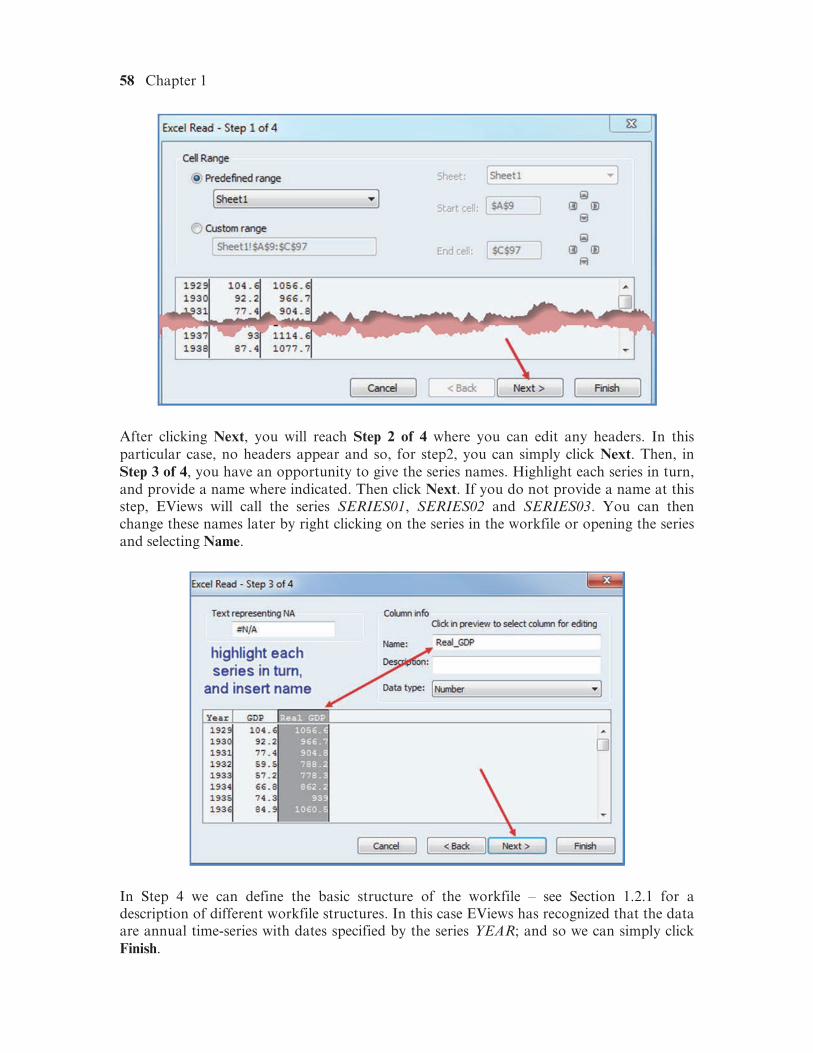
After clicking Next, you will reach Step 2 of 4 where you can edit any headers. In this particular case, no headers appear and so, for step2, you can simply click Next. Then, in Step 3 of 4, you have an opportunity to give the series names. Highlight each series in turn, and provide a name where indicated. Then click Next. If you do not provide a name at this step, EViews will call the series SERIES01, SERIES02 and SERIES03. You can then change these names later by right clicking on the series in the workfile or opening the series and selecting Name.
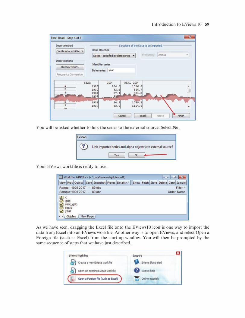
In Step 4 we can define the basic structure of the workfile – see Section 1.2.1 for a description of different workfile structures. In this case EViews has recognized that the data are annual time-series with dates specified by the series YEAR; and so we can simply click Finish.
Introduction to EViews 10 59
You will be asked whether to link the series to the external source. Select No.
Your EViews workfile is ready to use.
As we have seen, dragging the Excel file onto the EViews10 icon is one way to import the data from Excel into an EViews workfile. Another way is to open EViews, and select Open a Foreign file (such as Excel) from the start-up window. You will then be prompted by the same sequence of steps that we have just described.
60 Chapter 1
1.9.3 Importing other foreign files
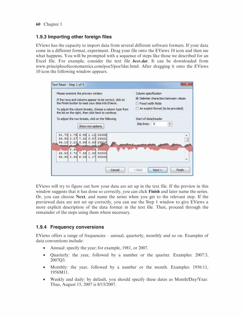
EViews has the capacity to import data from several different software formats. If your data come in a different format, experiment. Drag your file onto the EViews 10 icon and then see what happens. You will be prompted with a sequence of steps like those we described for an Excel file. For example, consider the text file beer.dat. It can be downloaded from www.principlesofeconometrics.com/poe5/poe5dat.html. After dragging it onto the EViews 10 icon the following window appears.
EViews will try to figure out how your data are set up in the text file. If the preview in this window suggests that it has done so correctly, you can click Finish and later name the series. Or, you can choose Next, and name the series when you get to the relevant step. If the previewed data are not set up correctly, you can use the Step 1 window to give EViews a more explicit description of the data format in the text file. Then, proceed through the remainder of the steps using them where necessary.
1.9.4 Frequency conversions
EViews offers a range of frequencies – annual, quarterly, monthly and so on. Examples of data conventions include:
• Annual: specify the year; for example, 1981, or 2007.
• Quarterly: the year, followed by a number or the quarter. Examples: 2007:3, 2007Q3.
• Monthly: the year, followed by a number or the month. Examples: 1956:11, 1956M11.
• Weekly and daily: by default, you should specify these dates as Month/Day/Year. Thus, August 15, 2007 is 8/15/2007.
Introduction to EViews 10 61
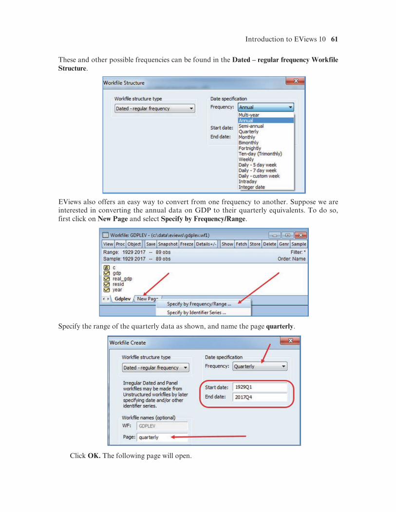
These and other possible frequencies can be found in the Dated – regular frequency Workfile Structure.
EViews also offers an easy way to convert from one frequency to another. Suppose we are interested in converting the annual data on GDP to their quarterly equivalents. To do so, first click on New Page and select Specify by Frequency/Range.
Specify the range of the quarterly data as shown, and name the page quarterly.
Click OK. The following page will open.
62 Chapter 1
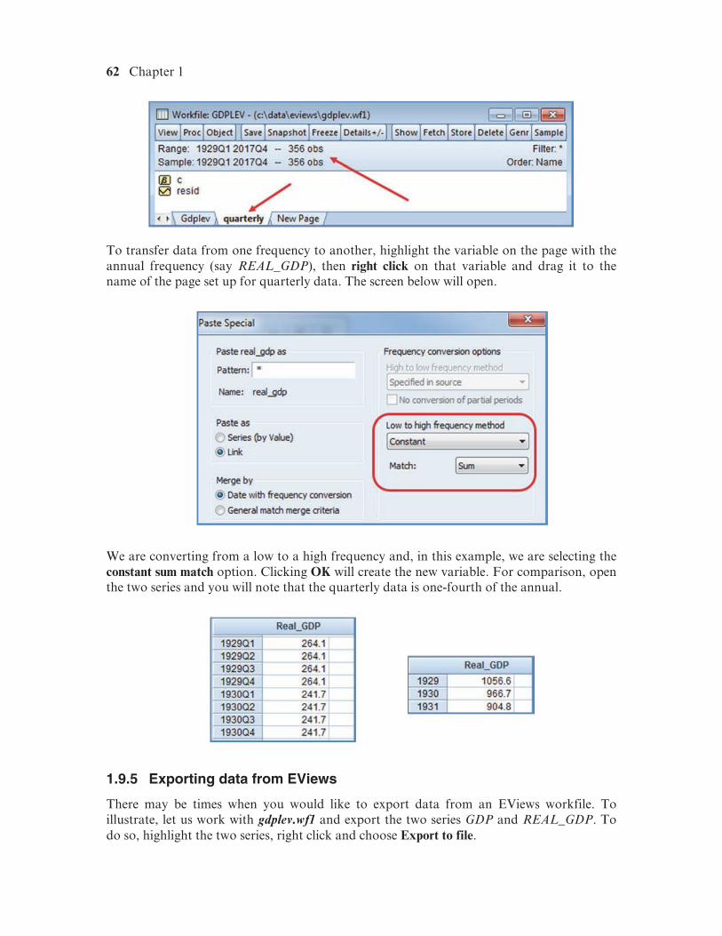
To transfer data from one frequency to another, highlight the variable on the page with the annual frequency (say REAL_GDP), then right click on that variable and drag it to the name of the page set up for quarterly data. The screen below will open.
We are converting from a low to a high frequency and, in this example, we are selecting the constant sum match option. Clicking OK will create the new variable. For comparison, open the two series and you will note that the quarterly data is one-fourth of the annual.
1.9.5 Exporting data from EViews
There may be times when you would like to export data from an EViews workfile. To illustrate, let us work with gdplev.wf1 and export the two series GDP and REAL_GDP. To do so, highlight the two series, right click and choose Export to file.
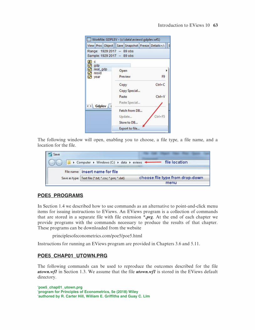
Introduction to EViews 10 63
The following window will open, enabling you to choose, a file type, a file name, and a location for the file.
POE5_PROGRAMS
In Section 1.4 we described how to use commands as an alternative to point-and-click menu items for issuing instructions to EViews. An EViews program is a collection of commands that are stored in a separate file with file extension *.prg. At the end of each chapter we provide programs with the commands necessary to produce the results of that chapter. These programs can be downloaded from the website
principlesofeconometrics.com/poe5/poe5.html
Instructions for running an EViews program are provided in Chapters 3.6 and 5.11.
POE5_CHAP01_UTOWN.PRG
The following commands can be used to reproduce the outcomes described for the file utown.wf1 in Section 1.3. We assume that the file utown.wf1 is stored in the EViews default directory. 'poe5_chap01_utown.prg 'program for Principles of Econometrics, 5e (2018) Wiley 'authored by R. Carter Hill, William E. Griffiths and Guay C. LIm
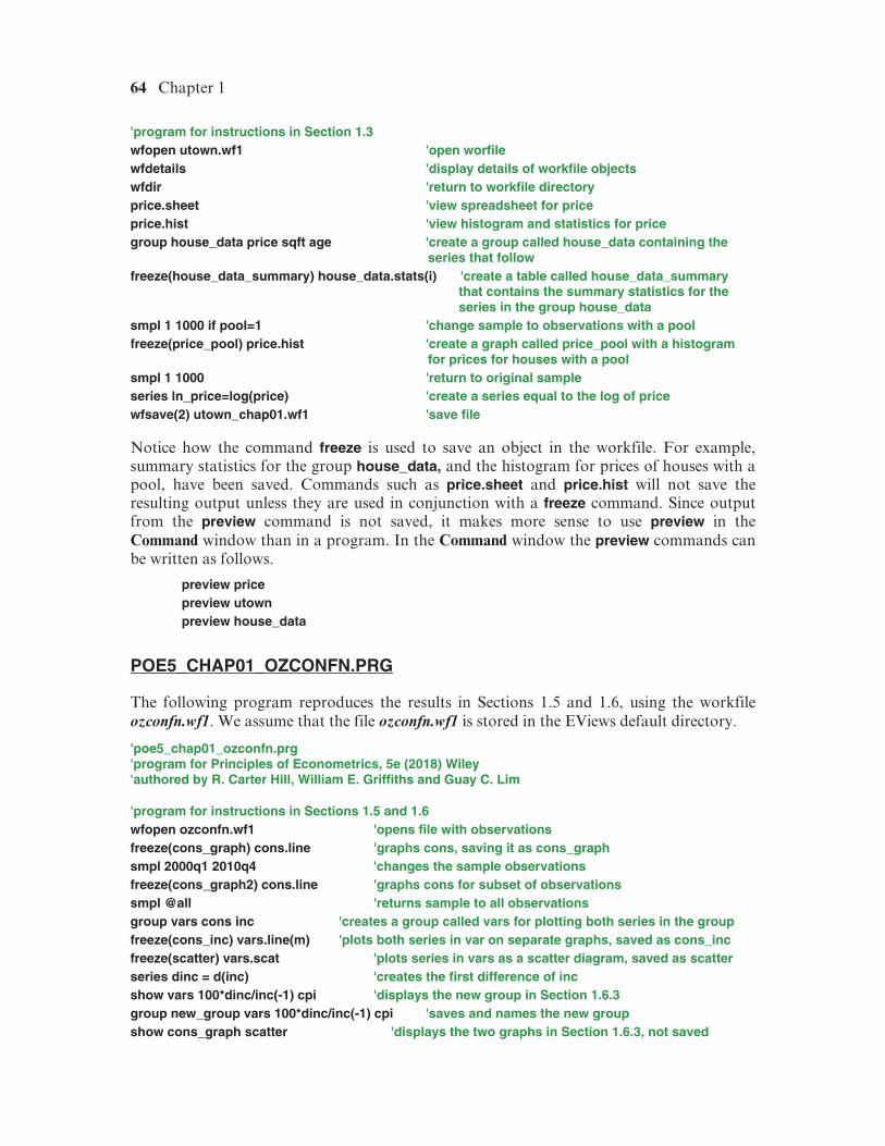
64 Chapter 1
'program for instructions in Section 1.3 wfopen utown.wf1 'open worfile wfdetails 'display details of workfile objects wfdir 'return to workfile directory price.sheet 'view spreadsheet for price price.hist 'view histogram and statistics for price group house_data price sqft age 'create a group called house_data containing the
series that follow freeze(house_data_summary) house_data.stats(i) 'create a table called house_data_summary
that contains the summary statistics for the series in the group house_data
smpl 1 1000 if pool=1 'change sample to observations with a pool freeze(price_pool) price.hist 'create a graph called price_pool with a histogram
for prices for houses with a pool smpl 1 1000 'return to original sample series ln_price=log(price) 'create a series equal to the log of price wfsave(2) utown_chap01.wf1 'save file
Notice how the command freeze is used to save an object in the workfile. For example, summary statistics for the group house_data, and the histogram for prices of houses with a pool, have been saved. Commands such as price.sheet and price.hist will not save the resulting output unless they are used in conjunction with a freeze command. Since output from the preview command is not saved, it makes more sense to use preview in the Command window than in a program. In the Command window the preview commands can be written as follows.
preview price preview utown preview house_data
POE5_CHAP01_OZCONFN.PRG
The following program reproduces the results in Sections 1.5 and 1.6, using the workfile ozconfn.wf1. We assume that the file ozconfn.wf1 is stored in the EViews default directory.
'poe5_chap01_ozconfn.prg 'program for Principles of Econometrics, 5e (2018) Wiley 'authored by R. Carter Hill, William E. Griffiths and Guay C. Lim
'program for instructions in Sections 1.5 and 1.6 wfopen ozconfn.wf1 'opens file with observations freeze(cons_graph) cons.line 'graphs cons, saving it as cons_graph smpl 2000q1 2010q4 'changes the sample observations freeze(cons_graph2) cons.line 'graphs cons for subset of observations smpl @all 'returns sample to all observations group vars cons inc 'creates a group called vars for plotting both series in the group freeze(cons_inc) vars.line(m) 'plots both series in var on separate graphs, saved as cons_inc freeze(scatter) vars.scat 'plots series in vars as a scatter diagram, saved as scatter series dinc = d(inc) 'creates the first difference of inc show vars 100*dinc/inc(-1) cpi 'displays the new group in Section 1.6.3 group new_group vars 100*dinc/inc(-1) cpi 'saves and names the new group show cons_graph scatter 'displays the two graphs in Section 1.6.3, not saved
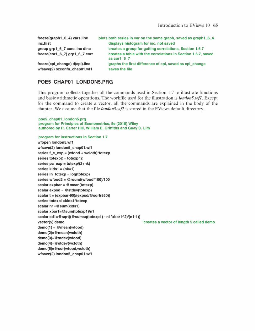
Introduction to EViews 10 65
freeze(graph1_6_4) vars.line 'plots both series in var on the same graph, saved as graph1_6_4 inc.hist 'displays histogram for inc, not saved group grp1_6_7 cons inc dinc 'creates a group for getting correlations, Section 1.6.7 freeze(cor1_6_7) grp1_6_7.corr 'creates a table with the correlations in Section 1.6.7, saved
as cor1_6_7 freeze(cpi_change) d(cpi).line 'graphs the first difference of cpi, saved as cpi_change wfsave(2) ozconfn_chap01.wf1 'saves the file
POE5_CHAP01_LONDON5.PRG
This program collects together all the commands used in Section 1.7 to illustrate functions and basic arithmetic operations. The workfile used for the illustration is london5.wf1. Except for the command to create a vector, all the commands are explained in the body of the chapter. We assume that the file london5.wf1 is stored in the EViews default directory. 'poe5_chap01_london5.prg 'program for Principles of Econometrics, 5e (2018) Wiley 'authored by R. Carter Hill, William E. Griffiths and Guay C. Lim 'program for instructions in Section 1.7 wfopen london5.wf1 wfsave(2) london5_chap01.wf1 series f_c_exp = (wfood + wcloth)*totexp series totexp2 = totexp^2 series pc_exp = totexp/(2+nk) series kids1 = (nk=1) series ln_totexp = log(totexp) series wfood2 = @round(wfood*100)/100 scalar expbar = @mean(totexp) scalar expsd = @stdev(totexp) scalar t = (expbar-90)/(expsd/@sqrt(850)) series totexp1=kids1*totexp scalar n1=@sum(kids1) scalar xbar1=@sum(totexp1)/n1 scalar sd1=@sqrt((@sumsq(totexp1) - n1*xbar1^2)/(n1-1)) vector(5) demo 'creates a vector of length 5 called demo demo(1) = @mean(wfood) demo(2)=@mean(wcloth) demo(3)=@stdev(wfood) demo(4)=@stdev(wcloth) demo(5)=@cor(wfood,wcloth) wfsave(2) london5_chap01.wf1