Embed Size (px)
Citation preview
Introduction to DEVS Modeling and Simulation with JAVA: Developing
Component-Based Simulation Models
Bernard P. Zeigler
Arizona Center for Integrative Modeling and Simulation
Electrical & Computer Enginering
College of Engineering and Mines
University of Arizona
Tucson, Arizona, USA
Hessam S. Sarjoughian
Arizona Center for Integrative Modeling and Simulation
Computer Science & Engineering
Fulton School of Engineering
Arizona State University
Tempe, Arizona, USA
January 2005
Copyright by the Authors
Draft Version 3
List of Chapters
Chapter 1..............................................................................................6
INTRODUCTION TO DEVS MODELING & SIMULATION METHODOLOGY........6 Framework for Modeling and Simulation ..............................................6
Brief Review of the DEVS Concepts ..................................................6 Basic Models .................................................................................8
Coupled Models .............................................................................9 Hierarchical Model Construction .....................................................10
The DEVS Formalism.......................................................................10 Classic DEVS System Specification .................................................10
Summary.......................................................................................12 Chapter 2............................................................................................13
WORKING WITH SIMPLE DEVS MODELS ...............................................13 DEVS SISO Models..........................................................................13
Passive.......................................................................................14 Storage ......................................................................................16 Generator ...................................................................................17 Binary Counter ............................................................................18
Ramp .........................................................................................19 Summary.......................................................................................20 Exercises.......................................................................................20
Solutions .......................................................................................21 Chapter 3............................................................................................26
DEVSJAVA CLASSES AND METHODS ....................................................26 Container Classes ...........................................................................26
DEVS Classes .................................................................................27 Class devs...................................................................................28 Class message.............................................................................29 Class atomic................................................................................30
Class coupled ..............................................................................31 Class digraph ..............................................................................31
Implementing the Single Input/Single Output DEVS ............................32 Class classic ................................................................................32
Class siso....................................................................................33
Table of Contents
3
Chapter 4............................................................................................34 PARALLEL DEVS MODELS IN DEVSJAVA................................................34
Parallel DEVS Basic Models ..............................................................34 Examples: Processor Models..........................................................35 Pseudo-code Example: Simple Processor.........................................35
Simple Processor Expressed in Parallel DEVS......................................38
Implementing the Simple Processor in DEVSJAVA ............................38 Another Example: Adding a Buffer to the Simple Processor ...............42 Processor with Random Processing Times........................................45 Processor Priority Queue...............................................................46
Models with Multiple Input and Output Ports ......................................48 DEVS Model of a Switch................................................................48 DEVSJAVA Implementation of the Switch........................................49
Sending/Receiving/Interpreting Messages..........................................51
More Atomic Models in DEVSJAVA.....................................................53 Storage with Ports for storing and retrieval .....................................53 Processor with (name, job) Input and Output Ports..........................54 Event List (Delay) Element............................................................55
Experimental Frame Components......................................................57 Stop/Start Generator....................................................................57 Generator of Time Consuming Jobs................................................58 Transducer..................................................................................59
Summary.......................................................................................62 Exercises.......................................................................................62 Solution.........................................................................................66
Chapter 5............................................................................................71
PARALLEL DEVS COUPLED MODELS .....................................................71 Coupled Models in the DEVS Formalism .............................................71
Component Requirements:............................................................71 Coupling Requirements:................................................................72
Example: Simple Pipeline.................................................................73 Implementing Coupled Models in DEVSJAVA.......................................74 The Behavior of Coupled Models .......................................................74 More Examples of Coupled Models ....................................................76
Switch Network ...........................................................................76 Generator/Processor/Transducer....................................................78
Table of Contents
4
Experimental Frame.....................................................................79 Hierarchical Models.........................................................................81
Implementing Hierarchical Models in DEVSJAVA...............................81 Summary.......................................................................................82 Exercises.......................................................................................82
Chapter 6............................................................................................84
EXERCISING MODELS: PARALLEL DEVS SIMULATION PROTOCOL ............84 Conservative and Optimistic Schemes ...............................................84
Simulating DEVS Models with Conservative and Optimistic Schemes...86 Parallel DEVS Simulation Protocol .....................................................87
Atomic Model Simulators...............................................................87 Coupled Model Coordinators..........................................................88 Expressing The Parallel DEVS Simulation Protocol as a Coupled Model 90
Summary.......................................................................................95
Exercises.......................................................................................95 Chapter 7............................................................................................97
MULTIPROCESSOR ARCHITECTURES....................................................97 Prototypical Processing Architectures.................................................97
Performance of Simple Architectures ..............................................98 Coordinators and Multiprocessor Architectures....................................99
Digraph Representation of the Architectures..................................100 Common Coordinator Class .........................................................100
Divide and Conquer.......................................................................102 Divide and Conquer Coordinator ..................................................103 Divide and Conquer Architecture..................................................105 Behavior of Divide and Conquer Architecture.................................105
Pipeline .......................................................................................106 Pipeline Coordinator ...................................................................106 Pipeline Architecture...................................................................109 Behavior of Pipeline....................................................................110
Multiserver...................................................................................111 Multiserver Coordinator ..............................................................111 Multiserver Architecture..............................................................113 Behavior of Multiserver...............................................................114
Turnaround Time and Throughput Relations for Series and Parallel Systems ......................................................................................116
Table of Contents
5
Families of Models.........................................................................116 Structural Inheritance.................................................................116
Range Inclusion Constraints on Coupling.......................................116 Homogeneous Coupled Models.....................................................118
Summary.....................................................................................118 Exercises.....................................................................................118
Solution.......................................................................................121 Solution.......................................................................................125
Chapter 8..........................................................................................129 SYSTEM ENTITY STRUCTURE ............................................................129
Model Base Management By System Entity Structure ........................130 System Entity Structure.................................................................132
System Entity-Structure/Model-Base (SES/MB) Framework.............133 Example: Design of a transaction processing system ......................134
Automatic Pruning of an SES.......................................................139 Implementation of the SES in DEVSJAVA.........................................140
SpecializationDEVS ....................................................................140 DEVSwithSpec...........................................................................140
Examples of the SES in DEVSJAVA...............................................142 Constraints on SpecializationDEVS and DEVSwithSpec....................146
Summary.....................................................................................147
Chapter 1
INTRODUCTION TO DEVS MODELING & SIMULATION METHODOLOGY
Framework for Modeling and Simulation
The Discrete Event System Specification (DEVS) formalism provides a means of specifying a mathematical object called a system. Basically, a system has a time base, inputs, states, and outputs, and functions for determining next states and outputs given current states and inputs. Discrete event systems represent certain constellations of such parameters just as continuous systems do. For example, the inputs in discrete event systems occur at arbitrarily spaced moments, while those in continuous systems are piecewise continuous functions of time. The insight provided by the DEVS formalism is in the simple way that it characterizes how discrete event simulation languages specify discrete event system parameters. Having this abstraction, it is possible to design new simulation languages with sound semantics that easier to understand. Indeed, the DEVJAVA environment to be described later is an implementation of the DEVS formalism in Java, which enables the modeler to specify models directly in its terms.
Brief Review of the DEVS Concepts
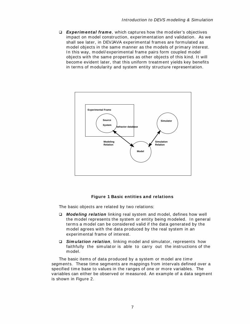
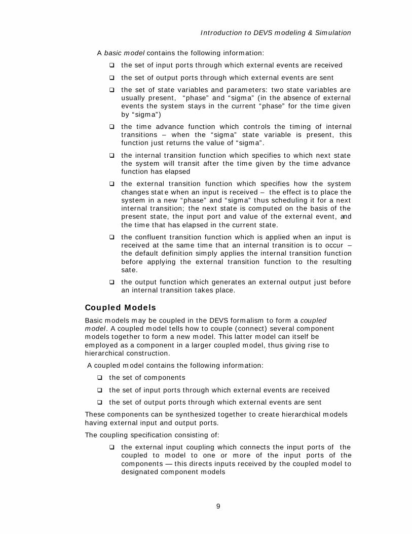
The conceptual framework underlying the DEVS formalism is shown in Figure 1. The modeling and simulation enterprise concerns three basic objects:
the Real system, in existence or proposed, which is regarded as fundamentally a source of data
q Model, which is a set of instructions for generating data comparable to that observable in the real system. The structure of the model is its set of instructions. The behavior of the model is the set of all possible data that can be generated by faithfully executing the model instructions.
q Simulator, which exercises the model's instructions to actually generate its behavior.
Introduction to DEVS modeling & Simulation
7
q Experimental frame, which captures how the modeler’s objectives impact on model construction, experimentation and validation. As we shall see later, in DEVJAVA experimental frames are formulated as model objects in the same manner as the models of primary interest. In this way, model/experimental frame pairs form coupled model objects with the same properties as other objects of this kind. It will become evident later, that this uniform treatment yields key benefits in terms of modularity and system entity structure representation.
Source
System
Simulator
Model
Experimental Frame
SimulationRelation
ModelingRelation
behavior database
Figure 1 Basic entities and relations
The basic objects are related by two relations:
q Modeling relation linking real system and model, defines how well the model represents the system or entity being modeled. In general terms a model can be considered valid if the data generated by the model agrees with the data produced by the real system in an experimental frame of interest.
q Simulation relation, linking model and simulator, represents how faithfully the simulator is able to carry out the instructions of the model.
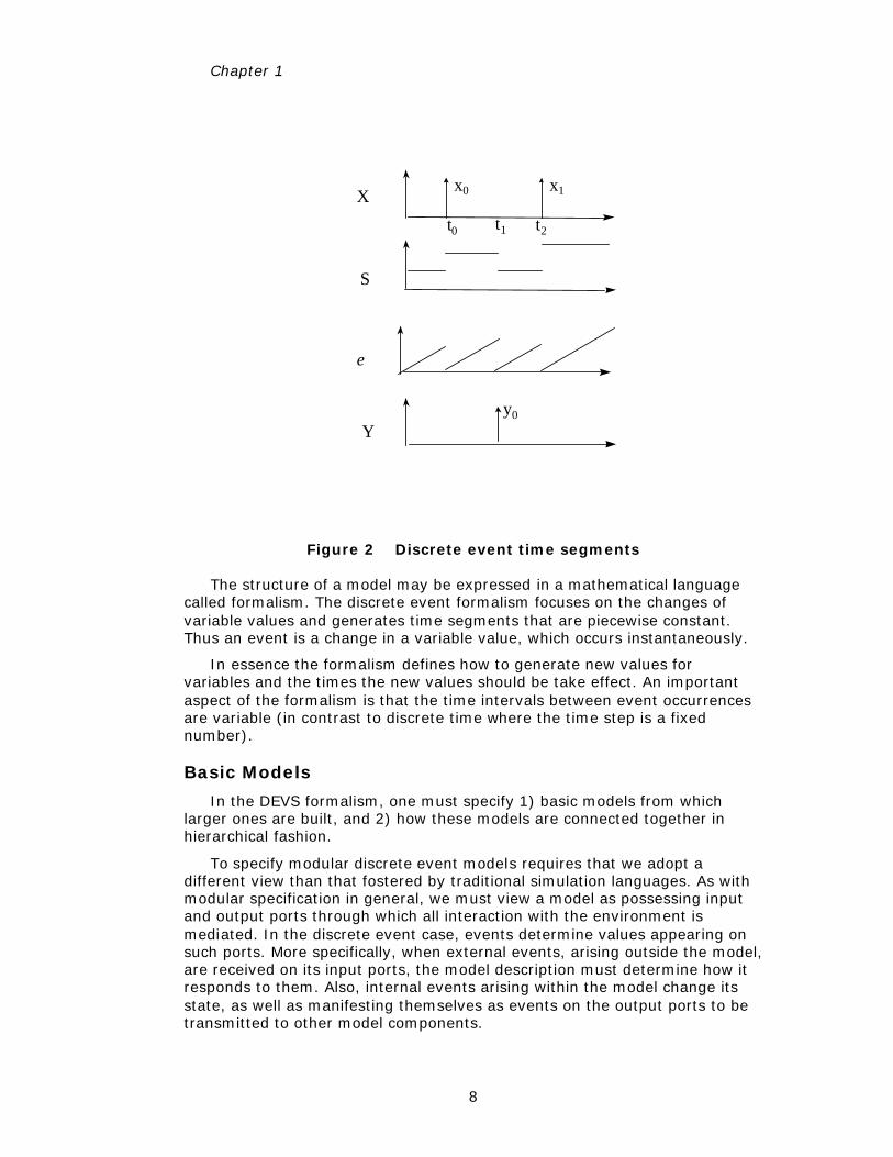
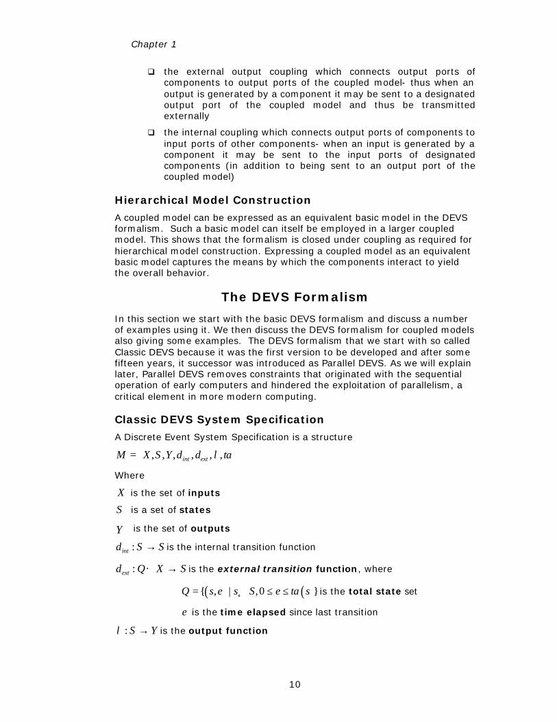
The basic items of data produced by a system or model are time segments. These time segments are mappings from intervals defined over a specified time base to values in the ranges of one or more variables. The variables can either be observed or measured. An example of a data segment is shown in Figure 2.
Chapter 1
8
x0 x1X
S
Yy0
e
t0 t1 t2
Figure 2 Discrete event time segments
The structure of a model may be expressed in a mathematical language called formalism. The discrete event formalism focuses on the changes of variable values and generates time segments that are piecewise constant. Thus an event is a change in a variable value, which occurs instantaneously.
In essence the formalism defines how to generate new values for variables and the times the new values should be take effect. An important aspect of the formalism is that the time intervals between event occurrences are variable (in contrast to discrete time where the time step is a fixed number).
Basic Models
In the DEVS formalism, one must specify 1) basic models from which larger ones are built, and 2) how these models are connected together in hierarchical fashion.
To specify modular discrete event models requires that we adopt a different view than that fostered by traditional simulation languages. As with modular specification in general, we must view a model as possessing input and output ports through which all interaction with the environment is mediated. In the discrete event case, events determine values appearing on such ports. More specifically, when external events, arising outside the model, are received on its input ports, the model description must determine how it responds to them. Also, internal events arising within the model change its state, as well as manifesting themselves as events on the output ports to be transmitted to other model components.
Introduction to DEVS modeling & Simulation
9
A basic model contains the following information:
q the set of input ports through which external events are received
q the set of output ports through which external events are sent
q the set of state variables and parameters: two state variables are usually present, “phase” and “sigma” (in the absence of external events the system stays in the current “phase” for the time given by “sigma”)
q the time advance function which controls the timing of internal transitions – when the “sigma” state variable is present, this function just returns the value of “sigma”.
q the internal transition function which specifies to which next state the system will transit after the time given by the time advance function has elapsed
q the external transition function which specifies how the system changes state when an input is received – the effect is to place the system in a new “phase” and “sigma” thus scheduling it for a next internal transition; the next state is computed on the basis of the present state, the input port and value of the external event, and the time that has elapsed in the current state.
q the confluent transition function which is applied when an input is received at the same time that an internal transition is to occur – the default definition simply applies the internal transition function before applying the external transition function to the resulting sate.
q the output function which generates an external output just before an internal transition takes place.
Coupled Models
Basic models may be coupled in the DEVS formalism to form a coupled model. A coupled model tells how to couple (connect) several component models together to form a new model. This latter model can itself be employed as a component in a larger coupled model, thus giving rise to hierarchical construction.
A coupled model contains the following information:
q the set of components
q the set of input ports through which external events are received
q the set of output ports through which external events are sent
These components can be synthesized together to create hierarchical models having external input and output ports.
The coupling specification consisting of:
q the external input coupling which connects the input ports of the coupled to model to one or more of the input ports of the components — this directs inputs received by the coupled model to designated component models
Chapter 1
10
q the external output coupling which connects output ports of components to output ports of the coupled model- thus when an output is generated by a component it may be sent to a designated output port of the coupled model and thus be transmitted externally
q the internal coupling which connects output ports of components to input ports of other components- when an input is generated by a component it may be sent to the input ports of designated components (in addition to being sent to an output port of the coupled model)
Hierarchical Model Construction
A coupled model can be expressed as an equivalent basic model in the DEVS formalism. Such a basic model can itself be employed in a larger coupled model. This shows that the formalism is closed under coupling as required for hierarchical model construction. Expressing a coupled model as an equivalent basic model captures the means by which the components interact to yield the overall behavior.
The DEVS Formalism
In this section we start with the basic DEVS formalism and discuss a number of examples using it. We then discuss the DEVS formalism for coupled models also giving some examples. The DEVS formalism that we start with so called Classic DEVS because it was the first version to be developed and after some fifteen years, it successor was introduced as Parallel DEVS. As we will explain later, Parallel DEVS removes constraints that originated with the sequential operation of early computers and hindered the exploitation of parallelism, a critical element in more modern computing.
Classic DEVS System Specification
A Discrete Event System Specification is a structure
, , , , , ,int extM X S Y taδ δ λ= ⟨ ⟩
Where
X is the set of inputs
S is a set of states
Y is the set of outputs
:int S Sδ → is the internal transition function
:ext Q X Sδ × → is the external transition function, where
( ) ( ){ , | ,0 }Q s e s S e ta s∈= ≤ ≤ is the total state set
e is the time elapsed since last transition
: S Yλ → is the output function
Introduction to DEVS modeling & Simulation
11
:ta S R+0,∞→ is the time advance function
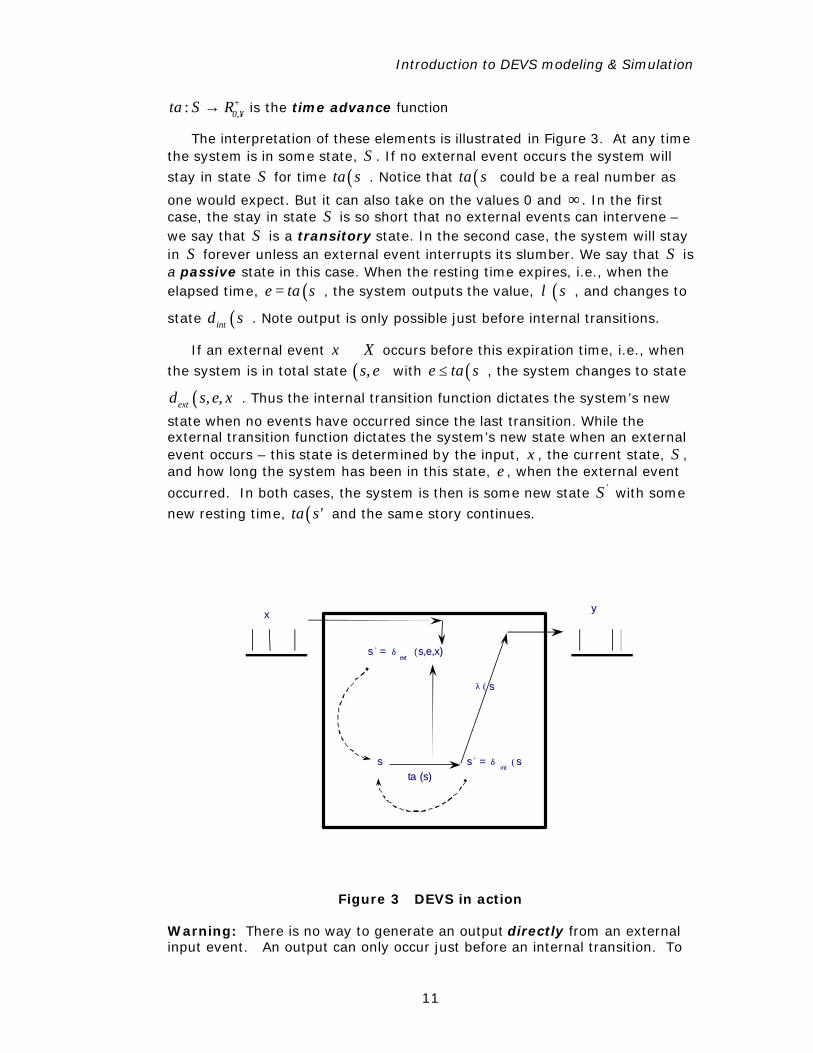
The interpretation of these elements is illustrated in Figure 3. At any time the system is in some state, S . If no external event occurs the system will
stay in state S for time ( )ta s . Notice that ( )ta s could be a real number as
one would expect. But it can also take on the values 0 and ∞ . In the first case, the stay in state S is so short that no external events can intervene – we say that S is a transitory state. In the second case, the system will stay in S forever unless an external event interrupts its slumber. We say that S is a passive state in this case. When the resting time expires, i.e., when the elapsed time, ( )e ta s= , the system outputs the value, ( )sλ , and changes to
state ( )int sδ . Note output is only possible just before internal transitions.
If an external event x ∈ X occurs before this expiration time, i.e., when
the system is in total state ( ),s e with ( )e ta s≤ , the system changes to state
( ), ,ext s e xδ . Thus the internal transition function dictates the system’s new
state when no events have occurred since the last transition. While the external transition function dictates the system’s new state when an external event occurs – this state is determined by the input, x , the current state, S , and how long the system has been in this state, e , when the external event
occurred. In both cases, the system is then is some new state 'S with some
new resting time, ( )ta s' and the same story continues.
xx yy
tata (s)(s)ss
λ (λ ( ss ))
ss ’ ’ = = δδintint
(( ss ))
ss ’ ’ = = δδextext
((s,e,x)s,e,x)
Figure 3 DEVS in action
Warning: There is no way to generate an output directly from an external input event. An output can only occur just before an internal transition. To
Chapter 1
12
have an external event cause an output without delay, we have it “schedule” an internal state with a hold time of zero. The relationship between external transitions, internal transitions, and outputs are as shown in Figure 3.
The above explanation of the semantics (or meaning) of a DEVS model suggests, but does not fully describe, the operation of a simulator that would execute such models to generate their behavior. We will delay discussion of such simulators to later chapters. However, the behavior of a DEVS is well defined and can be depicted as we mentioned earlier in Figure 2. In that figure, the input trajectory is a series of events occurring at times such as t0 and t2. In between, such event times may be those such as t1, which are times of internal events. The latter are noticeable on the state trajectory, which is a step-like series of states, which change at external and internal events (second from top). The elapsed time trajectory is a saw-tooth pattern depicting the flow of time in an elapsed time clock, which gets reset to 0 at every event. Finally, at the bottom, the output trajectory depicts the output events that are produced by the output function just before applying the internal transition function at internal events. Such behaviors will be illustrated in the next chapter.
Summary
The form of DEVS (discrete event system specification) discussed in this chapter provides a hierarchical, modular approach to constructing discrete event simulation models. In doing so, the DEVS formalism embodies the concepts of systems theory and modeling. We will see later, that DEVS is important not only for discrete event models, but also because it affords a computational basis for implementing behaviors that are expressed in DESS and DTSS, the other basic systems formalisms.
Chapter 2
WORKING WITH SIMPLE DEVS MODELS
Unlike many commercial packages, DEVS does not cater to a specific application domain, but is instead capable of expressing the full range of discrete event models. The downside of this capability is that the learning curve toward full DEVS modeling and simulation competence is steep. As a consequence, we’ll break up the presentation into several easier-to-bite pieces. First, we’ll discuss an artificially restricted class called siso (single input/single output) which deals only with single real values as input and output and does not allow juggling the values on multiple input and output ports. Subsequently, we’ll add the capability to work with Classic DEVS (multiple input and output ports, but only one input port event at a time). Finally, we’ll graduate to the full capability of Parallel DEVS. Think of this as learning to crawl in order to learn walk – after haven taken your first walk, you’ll be reluctant to return to crawling, but the latter serves as a necessary scaffold to get to the walking stage.
DEVS SISO Models
This chapter deals only with models that have only a single input and a single output, both expressed as real numbers. These models are implemented using the class siso as mentioned before. The table lists the models to be discussed in this chapter.
Models I/O Behavior Description
passive never generates output
storage stores the input and responds with it when queried
generator outputs a 1 in a periodic fashion
binaryCounter outputs a 1 only when it has received an even
Chapter 2
14
number of 1’s
ramp output acts like the position of a billiard ball that has been hit by the input
Table 1 Examples of DEVS SISO models
Passive
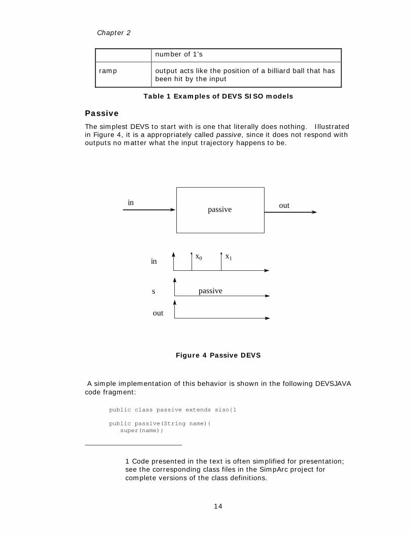
The simplest DEVS to start with is one that literally does nothing. Illustrated in Figure 4, it is a appropriately called passive, since it does not respond with outputs no matter what the input trajectory happens to be.
in outpassive
x0 x1in
s
out
passive
Figure 4 Passive DEVS
A simple implementation of this behavior is shown in the following DEVSJAVA code fragment:
public class passive extends siso{1 public passive(String name){ super(name);
1 Code presented in the text is often simplified for presentation; see the corresponding class files in the SimpArc project for complete versions of the class definitions.
Working with DEVS Models
15
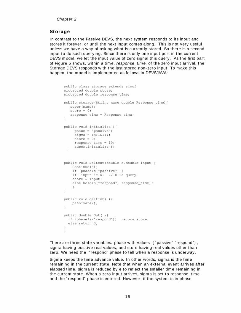
} public void initialize(){ phase = "passive"; sigma = INFINITY; super.initialize(); } public void Deltext(double e,double input){ passivate(); } public void deltint( ){ passivate(); } public double Out( ){ return 0; } }
The input and output sets are numerical. There is only one state “passive”. In this state, the time advance given by ta is infinite. As already indicated, this means the system will stay in passive forever unless interrupted by an input. However, in this model, even such an interruption will not awaken it, since the external transition function does disturb the state. The specifications of the internal transition and output functions are redundant here since they will never get a chance to be applied.
0
x1
respond
x1
response_time
respond
x1
0 x2
respond
x1
0 x2
sigma
x1
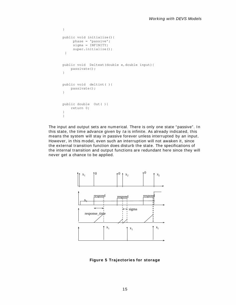
Figure 5 Trajectories for storage
Chapter 2
16
Storage
In contrast to the Passive DEVS, the next system responds to its input and stores it forever, or until the next input comes along. This is not very useful unless we have a way of asking what is currently stored. So there is a second input to do such querying. Since there is only one input port in the current DEVS model, we let the input value of zero signal this query. As the first part of Figure 5 shows, within a time, response_time, of the zero input arrival, the Storage DEVS responds with the last stored non-zero input. To make this happen, the model is implemented as follows in DEVSJAVA:
public class storage extends siso{ protected double store; protected double response_time; public storage(String name,double Response_time){ super(name); store = 0; response_time = Response_time; } public void initialize(){ phase = "passive"; sigma = INFINITY; store = 0; response_time = 10; super.initialize(); } public void Deltext(double e,double input){ Continue(e); if (phaseIs("passive")){ if (input != 0) // 0 is query store = input; else holdIn("respond", response_time); } } public void deltint( ){ passivate(); } public double Out( ){ if (phaseIs("respond")) return store; else return 0; } }
There are three state variables: phase with values {“passive“,“respond“}, sigma having positive real values, and store having real values other than zero. We need the “respond” phase to tell when a response is underway.
Sigma keeps the time advance value. In other words, sigma is the time remaining in the current state. Note that when an external event arrives after elapsed time, sigma is reduced by e to reflect the smaller time remaining in the current state. When a zero input arrives, sigma is set to response_time and the “respond” phase is entered. However, if the system is in phase
Working with DEVS Models
17
“respond” and an input arrives, the input is ignored as illustrated in the second part of Figure 2. When the response_time period has elapsed, the output function produces the stored value and the internal transition dictates a return to the passive state. What happens if, as in the third part of Figure 2, an input arrives just as the response period has elapsed? Classic DEVS and parallel DEVS differ in their ways of handling this collision as we shall show later.
active
period
1 11
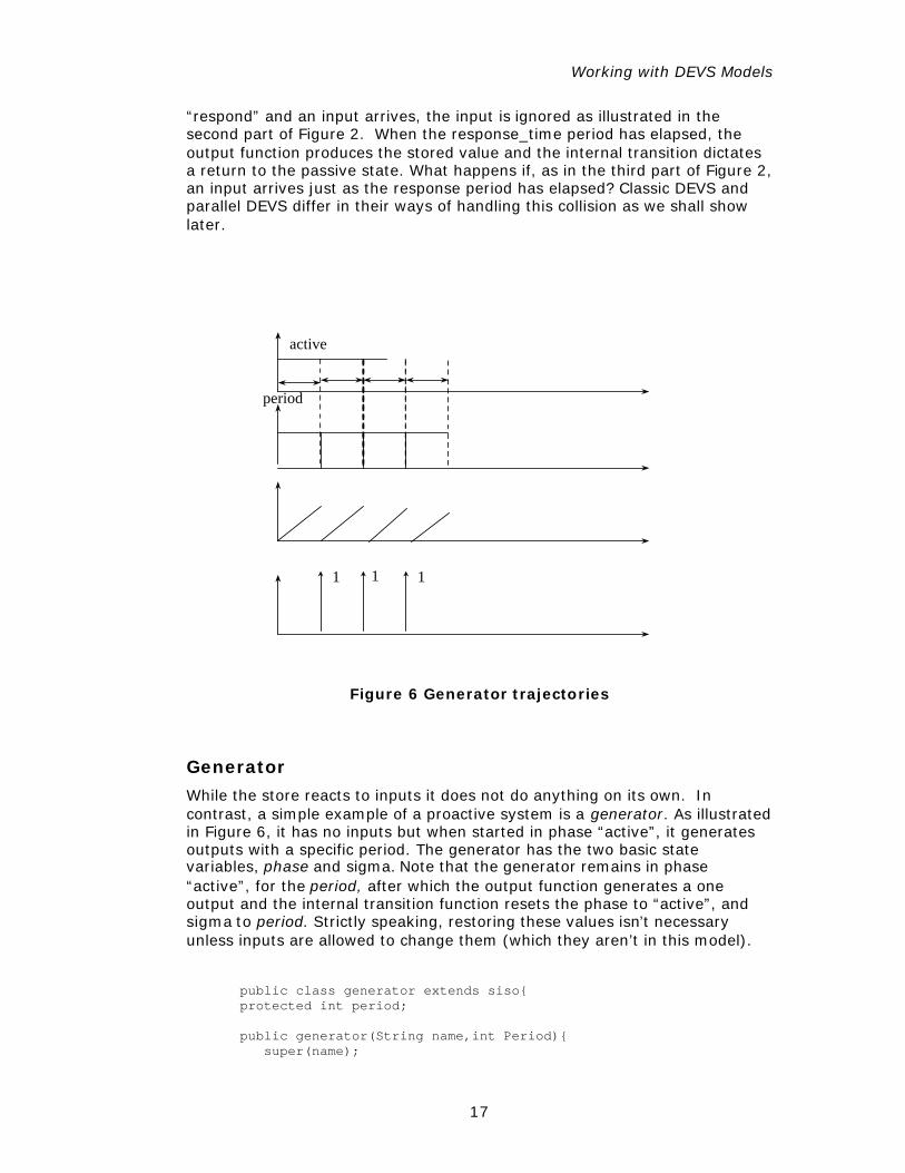
Figure 6 Generator trajectories
Generator
While the store reacts to inputs it does not do anything on its own. In contrast, a simple example of a proactive system is a generator. As illustrated in Figure 6, it has no inputs but when started in phase “active”, it generates outputs with a specific period. The generator has the two basic state variables, phase and sigma. Note that the generator remains in phase “active”, for the period, after which the output function generates a one output and the internal transition function resets the phase to “active”, and sigma to period. Strictly speaking, restoring these values isn’t necessary unless inputs are allowed to change them (which they aren’t in this model).
public class generator extends siso{ protected int period; public generator(String name,int Period){ super(name);
Chapter 2
18
period = Period; } public void initialize(){ phase = "active"; sigma = period; super.initialize(); } public void deltint( ){ holdIn("active",period); } public double Out( ){ return 1; } }
Binary Counter
In this example, the DEVS outputs a “one” for every two “one”s that it receives. To do this it maintains a count (modulo 2) of the “one”s it has received to date. When it receives a “one” that makes its count even, it goes into a transitory phase, “active”, to generate the output. This is the same as putting response_time: = 0 in the Storage DEVS.
public class binaryCounterSiso extends siso{ int count; public binaryCounterSiso(String name){ super(name); } public void initialize(){ count = 0; super.initialize(); } public void Deltext(double e,double input){ Continue(e); count = count + (int)input; if (count >= 2){ count = 0; holdIn("active",10); } } public void deltint( ){ passivate(); } public double Out( ){ if (phaseIs("active")) return 1; else return 0; } }
Working with DEVS Models
19
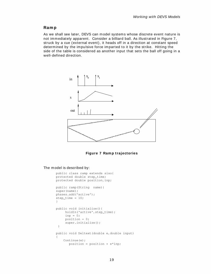
Ramp
As we shall see later, DEVS can model systems whose discrete event nature is not immediately apparent. Consider a billiard ball. As illustrated in Figure 7, struck by a cue (external event), it heads off in a direction at constant speed determined by the impulsive force imparted to it by the strike. Hitting the side of the table is considered as another input that sets the ball off going in a well-defined direction.
x0 x1in
s
out
Figure 7 Ramp trajectories
The model is described by: public class ramp extends siso{ protected double step_time; protected double position,inp; public ramp(String name){ super(name); phases.add("active"); step_time = 10; } public void initialize(){ holdIn("active",step_time); inp = 0; position = 0; super.initialize(); } public void Deltext(double e,double input) { Continue(e); position = position + e*inp;
Chapter 2
20
inp = input; } public void deltint( ) { position = position + sigma*inp; sigma = step_time; } public double Out( ) { double nextposition = position + sigma*inp; return nextposition; } }
The model stores its input and uses it as the value of the slope to compute the position of the ball (in a one-dimensional simplification). It outputs the current position every step_time. If it receives a new slope in the middle of a period, it updates the position to a value determined by the slope and elapsed time. Note that it outputs the position prevailing at the time of the output. This must be computed in the output function since it always called before the next internal event actually occurs. Note that we do not allow the output function to make this update permanent (using the temporary variable nextposition – which could also be absorbed directly into the return statement). The reason is that the output function is not allowed to change the state in the DEVS formalism.
Warning. A model in the output function changes the state of a model may produce unexpected and hard-to-locate errors because DEVS simulators do not guarantee correctness for models that do not conform to the given specification.
Summary
Working with a restricted version of DEVS allowed us to present some of the basic ideas underlying the construction of DEVS basic models. Although we used DEVSJAVA code to implement the model examples, we did so without describing the basic class structure that underlies this code. The next chapter will present this structure and show how the class siso is derived from it.
Exercises
Exercise 1: An nCounter generalizes the binary counter by generating a “one” for every n “one”s it receives. Specify an nCounter as a siso model in DEVS.
Exercise 2: Define a DEVS counter that counts the number of non-zero input events received since initialization and outputs this number when queried by a zero valued input.
Exercise 3:
Part a) Express in pseudo-code the one-dimensional ramp discussed in this chapter.
Working with DEVS Models
21
Part a) Implement the ramp model in DEVSJAVA, simulate it, and verify that its behavior is correct.
Exercise 4: For the billiard example, consider the more realistic situation where the position of the billiard ball is represented in a two dimensional space. For this revised system,
Part a) Develop its pseudo-code.
Part b) Write its DEVS specification.
Part c) Identify its appropriate input streams that allow the essential modes of behavior to be observed.
Part d) Implement the billiard ball model in DEVSJAVA.
Part e) Exercise the simulation model developed in (d) using the input streams identified in (c).
Solutions
Exercise 3:
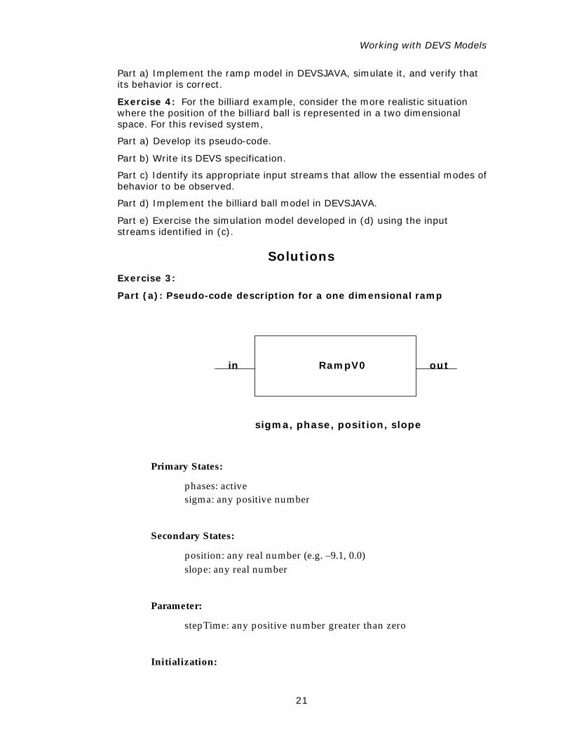
Part (a): Pseudo-code description for a one dimensional ramp
in RampV0 out
sigma, phase, position, slope
Primary States:
phases: active sigma: any positive number
Secondary States:
position: any real number (e.g. –9.1, 0.0) slope: any real number
Parameter:
stepTime: any positive number greater than zero
Initialization:
Chapter 2
22
phase = active sigma = any finite real number
External Transition Function:
When receive a new slope on input port “in” position = position + (e * slope) //update position according to e using the old slope slope = newSlope // update the slope sigma = sigma - e else //invalid input port names error
Internal Transition Function:
position = position + (sigma * slope) //update position according to sigma set sigma to stepTime //equivalent to hold-in(“active”, stepTime)
Output Function:
send position + (sigma * slope) to output port “out” // output the most up-to-date position
Exercise 4:
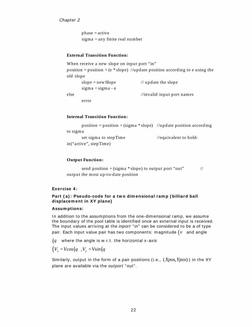
Part (a): Pseudo-code for a two dimensional ramp (billiard ball displacement in XY plane)
Assumptions:
In addition to the assumptions from the one-dimensional ramp, we assume the boundary of the pool table is identified once an external input is received. The input values arriving at the inport “in” can be considered to be a of type pair. Each input value pair has two components: magnitude ( )v and angle
( )θ where the angle is w.r.t. the horizontal x-axis
( ) ( )( ),x yV Vcos V Vsinθ θ= =
Similarly, output in the form of a pair positions (i.e., ( , )Xpos Ypos ) in the XY plane are available via the outport “out”.
Working with DEVS Models
23
Two Dimensional Ramp in out
sigma, phase,Xpos, Ypos, Vx, Vy
Part (b): pseudo-code for a two dimensional ramp (billiard ball)
Primary States:
phases: active sigma: any positive number
Secondary States:
Xpos: any real number Ypos: any real number Vx: any real number Vy: any real number
Parameter:
stepTime: any positive number greater than zero
Initialization:
Xpos = any finite real number Ypos = any finite real number Vx = any finite real number Vy = any finite real number
External Transition Function:
when receive entity v on input port “in” Xpos = Xpos + (e*Vx) //update position according to e using the old slope Ypos = Ypos + (e*Vy) Vx = v.V * cos(v.θ ) // update the slope Vy = v.V * sin(v.θ) phase = active
Chapter 2
24
sigma = sigma – e else //invalid input port names error
Internal Transition Function:
Xpos = Xpos + (sigma*Vx) Ypos = Ypos + (sigma*Vy) hold-in active for stepTime
Output Function:
send Xpos = Xpos + (sigma*Vx) and Ypos = Ypos + (sigma*Vy) as a value pair v = (Xpos, Ypos) to output port “out”
b) DEVS Specification
, , , , , ,int extDEVS X S Y taδ δ λ= ⟨ ⟩ where
// Dot notation is employed to obtain velocity ( )v and angle ( )θ for any
given input v (i.e., .vV and .vθ )
{" "}InPorts in ,=
{( , ) | , }X p v p InPorts v pair= ∈ ∈ is the set of input port and value pairs,
and {( , ) | , 0 360 }v V Vθ ℜ θ= ∈ ≤ ≤o o
{" "}OutPorts out ,=
{( , ) | , }pY p v p OutPorts v Y= ∈ ∈ is the set of output port and value
pairs,
and {( , ) | , };v Xpos Ypos Xpos Yposℜ ℜ= ∈ ∈
0{" "," "}S passive active × ℜ × ℜ × ℜ × ℜ × ℜ+=
( )( ), , , , , , , ,ext phase Vx Vy Xpos Ypos e p vδ σ =
( ) ( )( )" ", , . * . , . * . , * , * ;active e vV cos v vV sin v Xpos e Vx Ypos e Vyσ θ θ− + +
Working with DEVS Models
25
( , , , , , )ext phase Vx Vy Xpos Yposδ σ =
(" ", , , , * , * );active stepTime Vx Vy Xpos Vx Ypos Vyσ σ+ +
( , , , , , )phase Vx Vy Xpos Yposλ σ =
( )" ",out v where, . *v Xpos Xpos Vxσ= + and . * ;vYpos Ypos Vyσ= +
( ), , , , .ta phase Vx Vy Xpos Yposσ σ< =
Part (c): Input streams
Input events arriving with some non-zero inter-arrival time between them. The values of input events are:
Velocity (i.e., any real number) with 0 360θ≤ ≤o o with the following special cases:
Velocity (i.e., non-zero) in the X direction (i.e., 0θ = o or 180o)
Velocity (i.e., non-zero) in the Y direction (i.e., 90θ = o or 270o )
Chapter 3
DEVSJAVA CLASSES AND METHODS
Before going further, we will briefly discuss the implementation of DEVS in Java. A more complete description of the implementation is in the DEVSJAVA reference guide available from the web site www.acims.arizona.edu under Software. You will need to know the basic class hierarchy and methods to be able to write DEVS models in DEVSJAVA. We’ll close this chapter with a discussion of the implementation of the siso class, which will give you a little more insight into how both the generic devs classes and the siso class work.
Container Classes
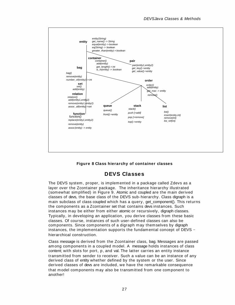
DEVSJAVA employs two packages to implement the DEVS concepts. Container classes, used to hold instances of objects, are implemented in the Package Zcontainer. The inheritance hierarchy of container classes is shown in Figure 1. The classes are roughly characterized as follows:
q entity - the base class for all classes of objects to be put into containers
q pair - holds a pair of entities called key and value
q container - the base class for container classes, provides basic services for the derived classes
q bag - counts numbers of object occurrences
q set - only one occurrence of any object is allowed in.
q relation - is a set of key-value pairs, used in dictionary fashion
q function - is a relation in which only one occurrence of any key allowed
q order - maintains items in given order
q queue - maintains items in first-in/first-out (FIFO) order
q stack - maintains items in last-in/first-out (LIFO) order
q list - maintains items in order determined by an insertion index
DEVSJava Classes & Methods
27
bag
function
set
relation
add(entity)
remove(entity1,entity2)
assoc(entity) -> entity
assoc_all(entity)->set
replace(entity1,entity2)
entity
add(entity1,entity2)
is_in(entity) -> boolean
container
add(entity)get_length()-> int
listqueue stack
insert(entity,int)
list_ref(int)remove(int)
front()->entity
order
top()->entity
pop [=remove]
push [=add]
greater_than(entity)-> boolean
get_max -> entity
pair
get_key()->entityget_value()->entity
container()
remove(entity)number_of(entity) -> int
bag()
set()
relation()
function()
remove(entity)
get_name() -> Stringequal(entity) -> boolean
entity(String)
eq(String) -> boolean
pair(entity1,entity2)
add(entity)order()
remove()
queue() stack()list()
Figure 8 Class hierarchy of container classes
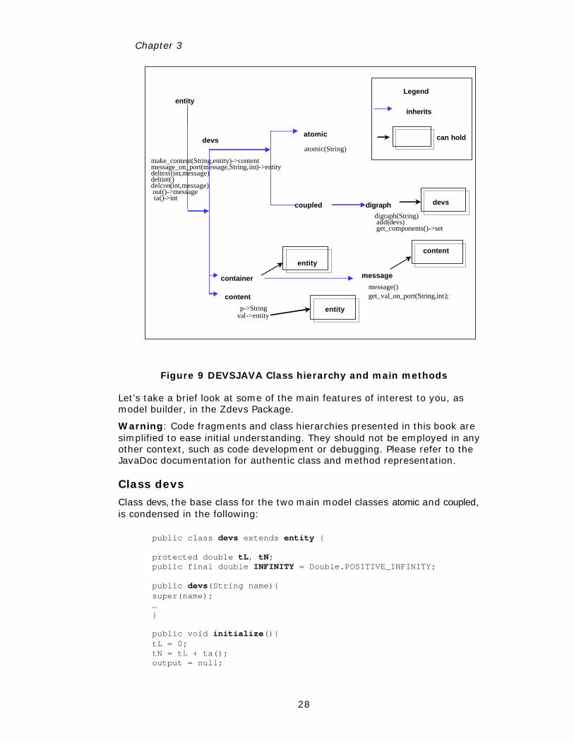
DEVS Classes
The DEVS system, proper, is implemented in a package called Zdevs as a layer over the Zcontainer package. The inheritance hierarchy illustrated (somewhat simplified) in Figure 9. Atomic and coupled are the main derived classes of devs, the base class of the DEVS sub-hierarchy. Class digraph is a main subclass of class coupled which has a query, get_component(). This returns the components as a Zcontainer set that contains devs instances. Such instances may be either from either atomic or recursively, digraph classes. Typically, in developing an application, you derive classes from these basic classes. Of course, instances of such user-defined classes can also be components. Since components of a digraph may themselves by digraph instances, the implementation supports the fundamental concept of DEVS − hierarchical construction.
Class message is derived from the Zcontainer class, bag. Messages are passed among components in a coupled model. A message holds instances of class content; with slots for port, p, and val. The latter carries an entity instance transmitted from sender to receiver. Such a value can be an instance of any derived class of entity whether defined by the system or the user. Since derived classes of devs are included , we have the remarkable consequence that model components may also be transmitted from one component to another!
Chapter 3
28
devs
entity
atomic
Legend
inherits
can hold
container message
content
content
atomic(String)
message()
p->Stringval->entity
make_content(String,entity)->contentmessage_on_port(message,String,int)->entitydeltext(int,message)deltint()delcon(int,message) out()->messageta()->int
digraph devs
get_components()->set add(devs)digraph(String)
entity
entity
coupled
get_val_on_port(String,int);
Figure 9 DEVSJAVA Class hierarchy and main methods
Let’s take a brief look at some of the main features of interest to you, as model builder, in the Zdevs Package.
Warning: Code fragments and class hierarchies presented in this book are simplified to ease initial understanding. They should not be employed in any other context, such as code development or debugging. Please refer to the JavaDoc documentation for authentic class and method representation.
Class devs
Class devs, the base class for the two main model classes atomic and coupled, is condensed in the following:
public class devs extends entity { protected double tL, tN; public final double INFINITY = Double.POSITIVE_INFINITY; public devs(String name){ super(name); … } public void initialize(){ tL = 0; tN = tL + ta(); output = null;
DEVSJava Classes & Methods
29
} public void inject(String p, entity val, double e){ message in = new message(); content co = makeContent(p, val); in.add(co); } public content makeContent(String p, entity value){ return new content(p,value); } public boolean messageOnPort(message x, String p, int i){ if (!inports.is_in_name(p)) System.out.println( "Warning: model :" + name + " inport: " + p + " has not been declared" ); return x.on_port(p, i); } }
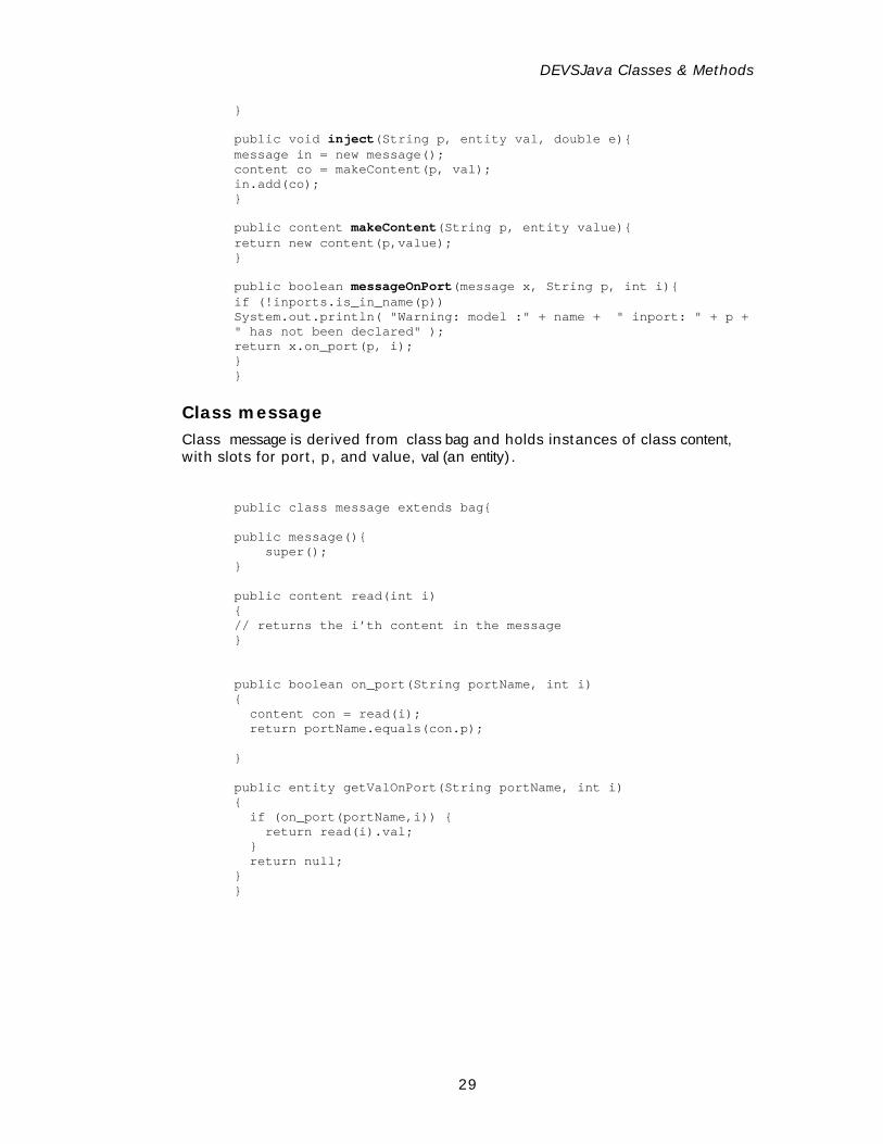
Class message Class message is derived from class bag and holds instances of class content, with slots for port, p, and value, val (an entity).
public class message extends bag{ public message(){ super(); } public content read(int i) { // returns the i’th content in the message } public boolean on_port(String portName, int i) { content con = read(i); return portName.equals(con.p); } public entity getValOnPort(String portName, int i) { if (on_port(portName,i)) { return read(i).val; } return null; } }
Chapter 3
30
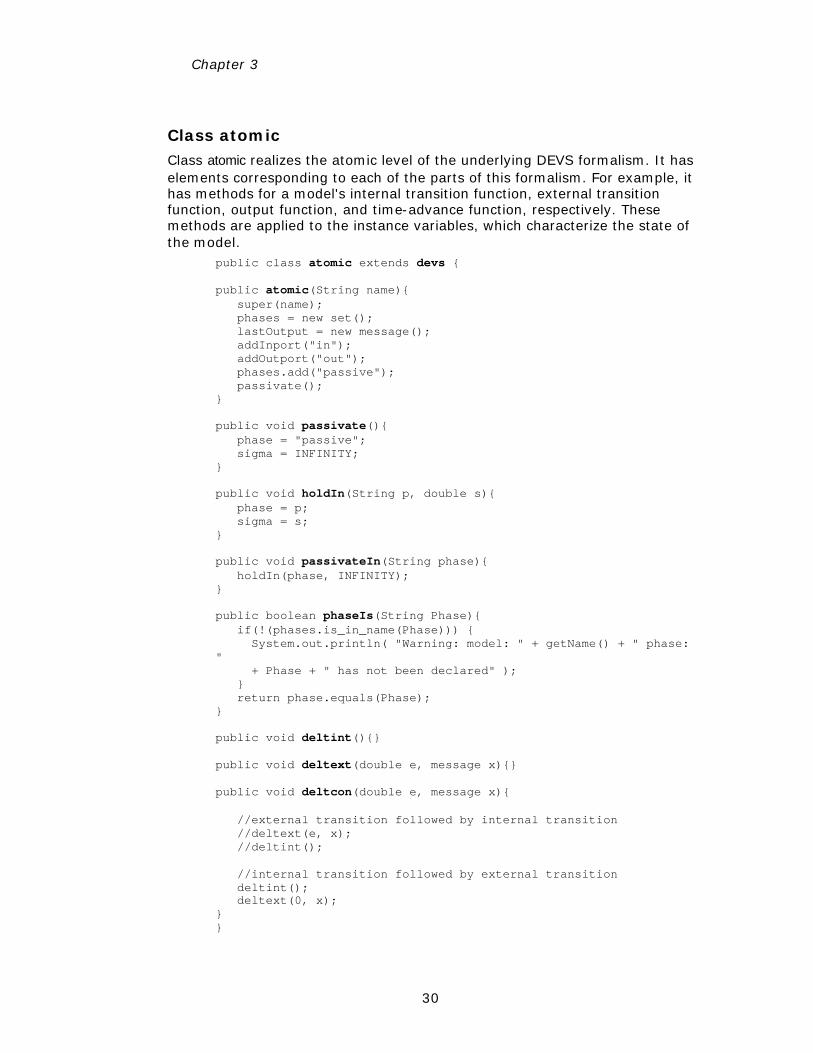
Class atomic Class atomic realizes the atomic level of the underlying DEVS formalism. It has elements corresponding to each of the parts of this formalism. For example, it has methods for a model's internal transition function, external transition function, output function, and time-advance function, respectively. These methods are applied to the instance variables, which characterize the state of the model.
public class atomic extends devs { public atomic(String name){ super(name); phases = new set(); lastOutput = new message(); addInport("in"); addOutport("out"); phases.add("passive"); passivate(); } public void passivate(){ phase = "passive"; sigma = INFINITY; } public void holdIn(String p, double s){ phase = p; sigma = s; } public void passivateIn(String phase){ holdIn(phase, INFINITY); } public boolean phaseIs(String Phase){ if(!(phases.is_in_name(Phase))) { System.out.println( "Warning: model: " + getName() + " phase: " + Phase + " has not been declared" ); } return phase.equals(Phase); } public void deltint(){} public void deltext(double e, message x){} public void deltcon(double e, message x){ //external transition followed by internal transition //deltext(e, x); //deltint(); //internal transition followed by external transition deltint(); deltext(0, x); } }
DEVSJava Classes & Methods
31
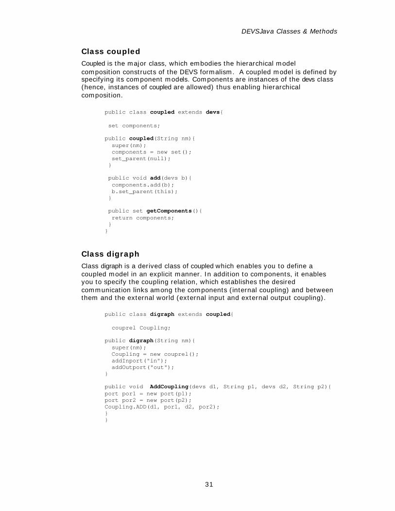
Class coupled Coupled is the major class, which embodies the hierarchical model composition constructs of the DEVS formalism. A coupled model is defined by specifying its component models. Components are instances of the devs class (hence, instances of coupled are allowed) thus enabling hierarchical composition.
public class coupled extends devs{ set components; public coupled(String nm){ super(nm); components = new set(); set_parent(null); } public void add(devs b){ components.add(b); b.set_parent(this); } public set getComponents(){ return components; } }
Class digraph Class digraph is a derived class of coupled which enables you to define a coupled model in an explicit manner. In addition to components, it enables you to specify the coupling relation, which establishes the desired communication links among the components (internal coupling) and between them and the external world (external input and external output coupling).
public class digraph extends coupled{ couprel Coupling; public digraph(String nm){ super(nm); Coupling = new couprel(); addInport("in"); addOutport("out"); } public void AddCoupling(devs d1, String p1, devs d2, String p2){ port por1 = new port(p1); port por2 = new port(p2); Coupling.ADD(d1, por1, d2, por2); } }
Chapter 3
32
Implementing the Single Input/Single Output DEVS
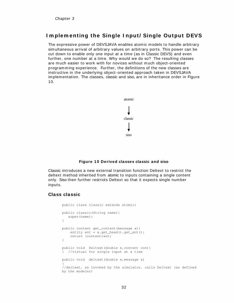
The expressive power of DEVSJAVA enables atomic models to handle arbitrary simultaneous arrival of arbitrary values on arbitrary ports. This power can be cut down to enable only one input at a time (as in Classic DEVS) and even further, one number at a time. Why would we do so? The resulting classes are much easier to work with for novices without much object-oriented programming experience. Further, the definitions of the new classes are instructive in the underlying object-oriented approach taken in DEVSJAVA implementation. The classes, classic and siso, are in inheritance order in Figure 10.
atomic
classic
siso
Figure 10 Derived classes classic and siso
Classic introduces a new external transition function Deltext to restrict the deltext method inherited from atomic to inputs containing a single content only. Siso then further restricts Deltext so that it expects single number inputs.
Class classic
public class classic extends atomic{ public classic(String name){ super(name); } public content get_content(message x){ entity ent = x.get_head().get_ent(); return (content)ent; } public void Deltext(double e,content con){ } //virtual for single input at a time public void deltext(double e,message x) { //deltext, as invoked by the simulator, calls Deltext (as defined by the modeler)
DEVSJava Classes & Methods
33
Deltext(e,get_content(x)); } }
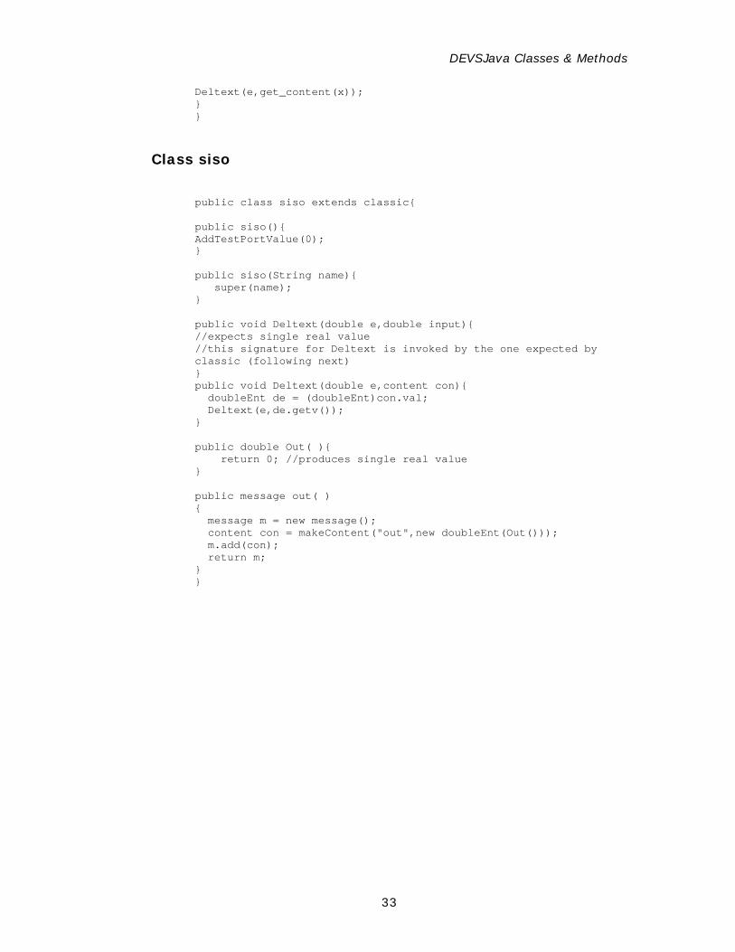
Class siso
public class siso extends classic{ public siso(){ AddTestPortValue(0); } public siso(String name){ super(name); } public void Deltext(double e,double input){ //expects single real value //this signature for Deltext is invoked by the one expected by classic (following next) } public void Deltext(double e,content con){ doubleEnt de = (doubleEnt)con.val; Deltext(e,de.getv()); } public double Out( ){ return 0; //produces single real value } public message out( ) { message m = new message(); content con = makeContent("out",new doubleEnt(Out())); m.add(con); return m; } }
Chapter 4
PARALLEL DEVS MODELS IN DEVSJAVA
Having discussed the basic classic hierarchy of DEVSJAVA we now are ready to start writing full-fledged models in its underlying formalism. Parallel DEVS differs from Classical DEVS in allowing all imminent components to be activated and to send their output to other components. The receiver is responsible for examining this input and properly interpreting it. Messages, basically lists of port - value pairs, are the basic exchange medium. This chapter discusses Parallel DEVS, and gives a variety of examples to contrast it with Classical DEVS.
Parallel DEVS Basic Models
A basic Parallel DEVS is a structure
( ), , , , , ,M M ext int conDEVS X Y S taδ ,δ δ λ=
where
{( , ) | , }MX p v p IPorts v Xp= ∈ ∈ is the set of input ports and values;
{( , ) | , }MY p v p OPorts v Yp= ∈ ∈ is the set of output ports and values;
S is the set of sequential states;
: bcon MQ X Sδ × → is the external state transition function;
int : S Sδ → is the internal state transition function;
: bcon MQ X Sδ × → is the confluent transition function;
: bS Yλ → is the output function;
0:ta S R+→ ∪ ∞ is the time advance function;
With : {( , ) | ,0 ( )}Q s e s S e ta s= ∈ ≤ ≤ the set of total states.
Parallel DEVS Coupled Models
35
We point out the important capabilities of Parallel DEVS beyond the classical DEVS formalism we presented earlier:
q Ports are represented explicitly – there can be any of input and output ports on which values can be received and sent
q Instead of receiving a single input or sending a single output, basic parallel DEVS models can handle bags of inputs and outputs. Recall that a bag can contain many elements with possibly multiple occurrences of its elements.
q We’ve added a transition function, called confluent. It decides the next state in cases of collision between external and internal events. We have seen examples of such collisions earlier in examining classical DEVS.
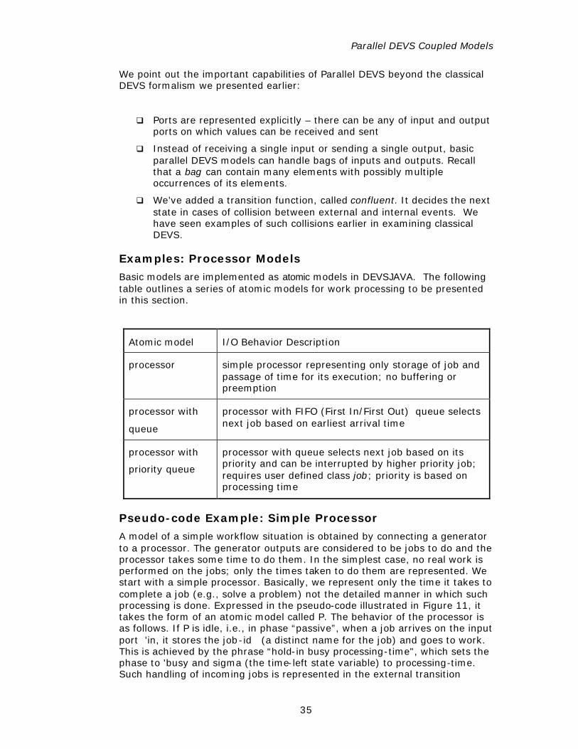
Examples: Processor Models
Basic models are implemented as atomic models in DEVSJAVA. The following table outlines a series of atomic models for work processing to be presented in this section.
Atomic model I/O Behavior Description
processor simple processor representing only storage of job and passage of time for its execution; no buffering or preemption
processor with
queue
processor with FIFO (First In/First Out) queue selects next job based on earliest arrival time
processor with
priority queue
processor with queue selects next job based on its priority and can be interrupted by higher priority job; requires user defined class job; priority is based on processing time
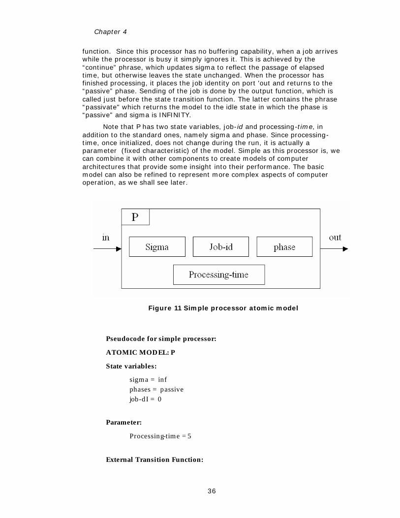
Pseudo-code Example: Simple Processor
A model of a simple workflow situation is obtained by connecting a generator to a processor. The generator outputs are considered to be jobs to do and the processor takes some time to do them. In the simplest case, no real work is performed on the jobs; only the times taken to do them are represented. We start with a simple processor. Basically, we represent only the time it takes to complete a job (e.g., solve a problem) not the detailed manner in which such processing is done. Expressed in the pseudo-code illustrated in Figure 11, it takes the form of an atomic model called P. The behavior of the processor is as follows. If P is idle, i.e., in phase “passive”, when a job arrives on the input port 'in, it stores the job-id (a distinct name for the job) and goes to work. This is achieved by the phrase “hold-in busy processing-time", which sets the phase to 'busy and sigma (the time-left state variable) to processing-time. Such handling of incoming jobs is represented in the external transition
Chapter 4
36
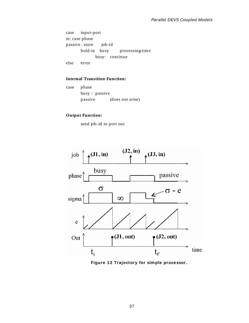
function. Since this processor has no buffering capability, when a job arrives while the processor is busy it simply ignores it. This is achieved by the “continue” phrase, which updates sigma to reflect the passage of elapsed time, but otherwise leaves the state unchanged. When the processor has finished processing, it places the job identity on port 'out and returns to the “passive” phase. Sending of the job is done by the output function, which is called just before the state transition function. The latter contains the phrase “passivate" which returns the model to the idle state in which the phase is “passive” and sigma is INFINITY.
Note that P has two state variables, job-id and processing-time, in addition to the standard ones, namely sigma and phase. Since processing-time, once initialized, does not change during the run, it is actually a parameter (fixed characteristic) of the model. Simple as this processor is, we can combine it with other components to create models of computer architectures that provide some insight into their performance. The basic model can also be refined to represent more complex aspects of computer operation, as we shall see later.
Figure 11 Simple processor atomic model
Pseudocode for simple processor:
ATOMIC MODEL: P
State variables:
sigma = inf phases = passive job-dI = 0
Parameter:
Processing-time = 5
External Transition Function:
Parallel DEVS Coupled Models
37
case input-port in: case phase passive : store job-id hold-in busy processing-time busy: continue else error
Internal Transition Function:
case phase busy : passive passive (does not arise)
Output Function:
send job-id to port out
Figure 12 Trajectory for simple processor.
Chapter 4
38
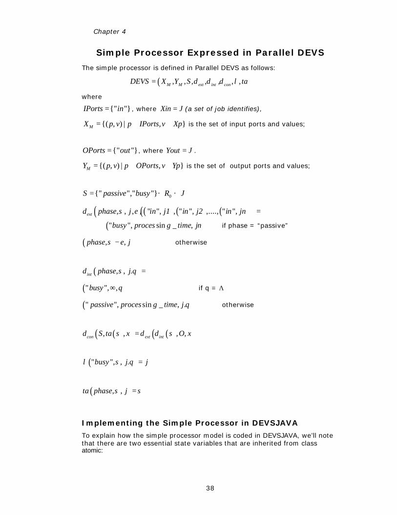
Simple Processor Expressed in Parallel DEVS
The simple processor is defined in Parallel DEVS as follows:
( ), , , , , , ,M M ext int conDEVS X Y S taδ δ δ λ=
where
{" "}IPorts in= , where Xin J= (a set of job identifies),
{( , ) | , }MX p v p IPorts v Xp= ∈ ∈ is the set of input ports and values;
{" "}OPorts out= , where Yout J= .
{( , ) | , }MY p v p OPorts v Yp= ∈ ∈ is the set of output ports and values;
0{" "," "}S passive busy R J× ×+=
( ) ( ) ( )( )( ), , , , " ", , " ", ,...., " ",ext phase j e in j1 in j2 in jnδ σ =
( )" ", sin _ ,busy proces g time jn if phase = “passive”
( ), ,phase e jσ − otherwise
( ), , .int phase j qδ σ =
( )" ", ,busy q∞ if q = Λ
( )" ", sin _ , .passive proces g time j q otherwise
( )( ) ( )( ), , , ,con ext intS ta s x s O xδ δ δ=
( )" ", , .busy j q jλ σ =
( ), ,ta phase jσ σ=
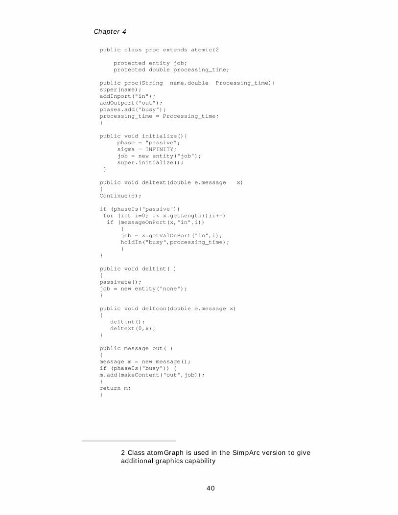
Implementing the Simple Processor in DEVSJAVA
To explain how the simple processor model is coded in DEVSJAVA, we’ll note that there are two essential state variables that are inherited from class atomic:

Parallel DEVS Coupled Models
39
q Phase is a control state that is almost always used in models to help keep track of where the full state is;
q Sigma holds the time remaining to the next internal event. This is precisely the time-advance value to be produced by the time-advance function.
The simple process class proc is defined as follows:
Chapter 4
40
2 Class atomGraph is used in the SimpArc version to give additional graphics capability
public class proc extends atomic{2 protected entity job; protected double processing_time; public proc(String name,double Processing_time){ super(name); addInport("in"); addOutport("out"); phases.add("busy"); processing_time = Processing_time; } public void initialize(){ phase = "passive"; sigma = INFINITY; job = new entity("job"); super.initialize(); } public void deltext(double e,message x) { Continue(e); if (phaseIs("passive")) for (int i=0; i< x.getLength();i++) if (messageOnPort(x,"in",i)) { job = x.getValOnPort("in",i); holdIn("busy",processing_time); } } public void deltint( ) { passivate(); job = new entity("none"); } public void deltcon(double e,message x) { deltint(); deltext(0,x); } public message out( ) { message m = new message(); if (phaseIs("busy")) { m.add(makeContent("out",job)); } return m; }
Parallel DEVS Coupled Models
41
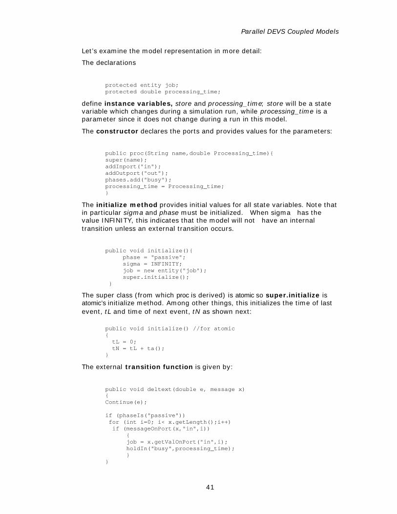
Let’s examine the model representation in more detail:
The declarations
protected entity job; protected double processing_time;
define instance variables, store and processing_time; store will be a state variable which changes during a simulation run, while processing_time is a parameter since it does not change during a run in this model.
The constructor declares the ports and provides values for the parameters:
public proc(String name,double Processing_time){ super(name); addInport("in"); addOutport("out"); phases.add("busy"); processing_time = Processing_time; }
The initialize method provides initial values for all state variables. Note that in particular sigma and phase must be initialized. When sigma has the value INFINITY, this indicates that the model will not have an internal transition unless an external transition occurs.
public void initialize(){ phase = "passive"; sigma = INFINITY; job = new entity("job"); super.initialize(); }
The super class (from which proc is derived) is atomic so super.initialize is atomic’s initialize method. Among other things, this initializes the time of last event, tL and time of next event, tN as shown next:
public void initialize() //for atomic { tL = 0; tN = tL + ta(); }
The external transition function is given by:
public void deltext(double e, message x) { Continue(e); if (phaseIs("passive")) for (int i=0; i< x.getLength();i++) if (messageOnPort(x,"in",i)) { job = x.getValOnPort("in",i); holdIn("busy",processing_time); } }
Chapter 4
42
The internal transition function is given by:
public void deltint( ){ passivate(); }
This states that the model will passivate (set sigma to INFINITY) after spending the time required in “busy. ”
The confluent transition function is given by:
public void deltcon(double e,message x){ deltint(); deltext(0,x); }
This is the default definition provided by the atomic class so could have been inherited without redefinition. We repeat it here to prepare the way for the discussion of collisions in the next chapter.
The output function is given by:
public message out( ) { message m = new message(); if (phaseIs("busy")) { m.add(makeContent("out",job)); } return m; }
This function first check if the phase equals “busy”; if so, an output on port “out” will be generated, otherwise a null message will be generated.
Another Example: Adding a Buffer to the Simple Processor
A processor that has a buffer is defined in Parallel DEVS as follows:
( ), , , , , , ,processing_time M M ext int conDEVS X Y S taδ δ δ λ=
where
{" "}InPorts in= , where Xin V= (an arbitrary set),
{( , ) | , }MX p v p IPorts v Xp= ∈ ∈ is the set of input ports and values;
{" "}OPorts out= , where Yout V= (an arbitrary set),
{( , ) | , }MY p v p OPorts v Yp= ∈ ∈ is the set of output ports and values;
Parallel DEVS Coupled Models
43
0{" "," "}S passive busy R V× ×+ +=
( ) ( ) ( )( )( ), , , , " ", , " ", ,...., " ",ext phase q e in x1 in x2 in xnδ σ =
( )" ", , , 2,....,busy processing_time x1 x xn if phase = “passive”
( ), , . , 2,....,phase e q x1 x xnσ − otherwise
( ), , .int phase v qδ σ =
( )" ", ,busy q∞ if q = Λ
( )" ", , .passive processing_time v q else
( )( ) ( )( ), , , ,con ext intS ta s x s O xδ δ δ=
( )" ", , .busy v q vλ σ =
( ), ,ta phase qσ σ=
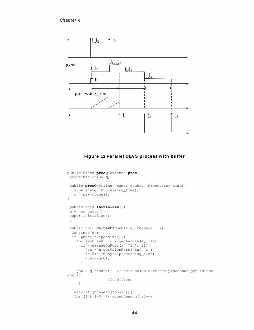
Using its buffer the processor can store jobs that arrive while it is busy. The buffer, also called a queue, is represented by a sequence of jobs, x1…xn in
V+ (the set of finite sequences of elements of V where Λ denotes the empty sequence). Jobs are processed in the order of arrival − i.e., first in first out (FIFO) order. In parallel DEVS, the processor can also handle jobs that arrive simultaneously on in its input port. These are placed in its queue and it starts working on the one it has selected to be first. Note that bags, like sets, are not ordered so there is no ordering of the jobs in the input bag. For convenience we have shown the job, which is first in the written order in δext as the one selected as the one to be processed. Figure 13 ustrates the concurrent arrival of two jobs and the subsequent arrival of a third just as the first job is about to be finished. Note that the confluent function, δcon specifies that the internal transition function is to be applied first. Thus, the job in process completes and exists. Then the external function adds the third job to the end of the queue and starts working on the second job. Classic DEVS has a hard time doing all this as easily!
Chapter 4
44
j1,j2queue
j1
processing_time
j3j1,j2
j1,j2,j3j2,j3
j2 j3
j3j1
Figure 13 Parallel DEVS process with buffer
public class procQ extends proc{ protected queue q; public procQ(String name, double Processing_time){ super(name, Processing_time); q = new queue(); } public void initialize(){ q = new queue(); super.initialize(); } public void deltext(double e, message x){ Continue(e); if (phaseIs("passive")){ for (int i=0; i< x.getLength(); i++) if (messageOnPort(x, "in", i)){ job = x.getValOnPort("in", i); holdIn("busy", processing_time); q.add(job); } job = q.front(); // this makes sure the processed job is the one at //the front } else if (phaseIs("busy")){ for (int i=0; i< x.getLength();i++)
Parallel DEVS Coupled Models
45
if (messageOnPort(x, "in", i)) { entity jb = x.getValOnPort("in", i); q.add(jb); } } } public void deltint( ){ q.remove(); if(!q.empty()){ job = q.front(); holdIn("busy", processing_time); } else passivate(); } // public message output( ){inherited from proc} }
Discrete-event simulation is often associated with simulation of queuing models and one might imagine that queuing is an inevitable factor in any such model. However, as new approaches to manufacturing such as just-in-time production have shown, queues are evidence of inadequate process co-ordination and impose a costly overhead that often can be avoided. In the models to be discussed in this book, we intentional ly do not incorporate queues, in favor of more sophisticated co-ordination schemes. The reader may wish to compare performance of the models in the ensuing chapters with, and without, queues. Modularity, and model base concepts, facilitates exploration of such alternatives.
Processor with Random Processing Times
The processor models discussed so far can be made more realistic in a variety of ways. Often the processing time in such a model is not constant but is sampled from a probability distribution probability distribution. This is easy to arrange in DEVSJAVA by modifying the external transition function. Distributions such as the exponential or normal may be used as explained in many books on discrete-event simulation.
holdIn("busy", exponential(100, 2);
(See section “Generator of Time Consuming Jobs” for details on the use of random number generators and probability distributions in DEVSJAVA.)
Chapter 4
46
Processor Priority Queue
public class job extends entity{ public double processing_time; public job(String name, double Processing_time){ super(name); processing_time = Processing_time; } public boolean greater_than( entity m){ job jm = (job)m; return processing_time < jm.processing_time; //choose on basis of smaller time left } public void update(double e){ processing_time = processing_time - e; } }
Parallel DEVS Coupled Models
47
public class priorityQ extends proc{ protected job jb; protected order q; public void initialize(){ q = new order(); jb = new job("nullJob"); super.initialize(); } public void deltext(int e,message x) { Continue(e); if (phaseIs("passive")) { for (int i=0; i< x.getLength();i++) if (messageOnPort(x,"in",i)) { entity ent = x.getValOnPort("in",i); q.add(ent); } entity ent = q.get_max(); jb = (job)ent; holdIn("busy",jb.processing_time); } else if (phaseIs("busy")) { jb.update(e); //update current job for (int i=0; i< x.getLength();i++) if (messageOnPort(x,"in",i)) { entity ent = x.getValOnPort("in",i); q.add(ent); } entity ent = q.get_max(); job max = (job)ent; if (jb != max){ jb = max; holdIn("busy",jb.processing_time); } } } public void deltint( ) { q.remove(); if(!q.empty()){ jb = (job)q.get_max(); holdIn("busy",jb.processing_time); } else passivate(); } public message out( ) { message m = new message(); if (phaseIs("busy")){ content con = makeContent("out",jb); m.add(con); } return m; } }
Chapter 4
48
Models with Multiple Input and Output Ports
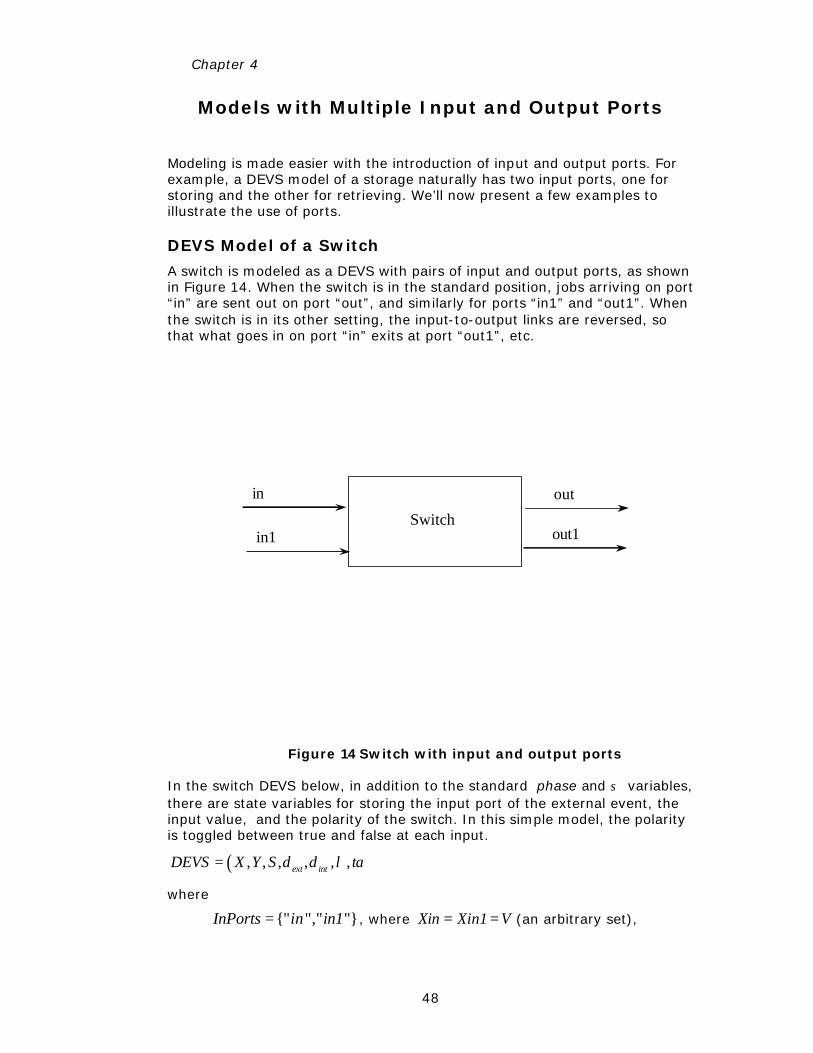
Modeling is made easier with the introduction of input and output ports. For example, a DEVS model of a storage naturally has two input ports, one for storing and the other for retrieving. We’ll now present a few examples to illustrate the use of ports.
DEVS Model of a Switch
A switch is modeled as a DEVS with pairs of input and output ports, as shown in Figure 14. When the switch is in the standard position, jobs arriving on port “in” are sent out on port “out”, and similarly for ports “in1” and “out1”. When the switch is in its other setting, the input-to-output links are reversed, so that what goes in on port “in” exits at port “out1”, etc.
in out
Switchin1 out1
Figure 14 Switch with input and output ports
In the switch DEVS below, in addition to the standard phase and σ variables, there are state variables for storing the input port of the external event, the input value, and the polarity of the switch. In this simple model, the polarity is toggled between true and false at each input.
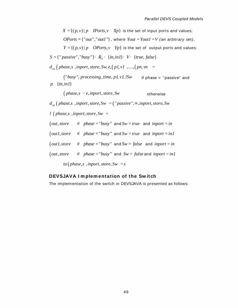
( ), , , , , ,ext intDEVS X Y S taδ δ λ=
where
{" "," "}InPorts in in1= , where Xin Xin1 V= = (an arbitrary set),
Parallel DEVS Coupled Models
49
{( , ) | , }X p v p IPorts v Xp= ∈ ∈ is the set of input ports and values;
{" "," "}OPorts out out1= , where Yout Yout1 V= = (an arbitrary set),
{( , ) | , }Y p v p OPorts v Yp= ∈ ∈ is the set of output ports and values;
0{" "," "} { , } { , }S passive busy R in in1 V true false× × × ×+=
( ) ( )( ), , , , , , , ,...., ,ext phase inport store Sw e p1 v1 pn vnδ σ =
( )" ", , , ,busy processing_time p1 v1 !Sw if phase = “passive” and
{ , }p in in1∈
( ), , , ,phase e inport store Swσ − otherwise
( ) ( ), , , , " ", , , ,int phase inport store Sw passive inport store Swδ σ = ∞
( ), , , ,phase inport store Swλ σ =
( ),out store if " "phase busy= andSw true= and inport in=
( ),out1 store if " "phase busy= andSw true= and inport in1=
( ),out1 store if " "phase busy= andSw false= and inport in=
( ),out store if " "phase busy= and Sw false= and inport in1=
( ), , , ,ta phase inport store Swσ σ=
DEVSJAVA Implementation of the Switch
The implementation of the switch in DEVSJAVA is presented as follows:
Chapter 4
50
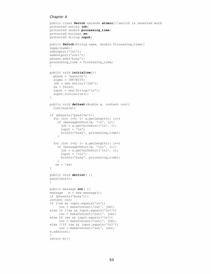
public class Switch extends atomic{//switch is reserved word protected entity job; protected double processing_time; protected boolean sw; protected String input; public Switch(String name, double Processing_time){ super(name); addInport("in1"); addOutport("out1"); phases.add("busy"); processing_time = Processing_time; } public void initialize(){ phase = "passive"; sigma = INFINITY; job = new entity("job"); sw = false; input = new String("in"); super.initialize(); } public void deltext(double e, content con){ Continue(e); if (phaseIs("passive")){ for (int i=0; i< x.getLength(); i++) if (messageOnPort(x, "in", i)){ job = x.getValOnPort("in", i); input = "in"; holdIn("busy", processing_time); } for (int i=0; i< x.getLength(); i++) if (messageOnPort(x, "in1", i)){ job = x.getValOnPort("in1", i); input = "in1"; holdIn("busy", processing_time); } sw = !sw; } public void deltint( ){ passivate(); } public message out( ){ message m = new message(); if (phaseIs("busy")){ content con; if (!sw && input.equals("in")) con = makeContent("out", job); else if (!sw && input.equals("in1")) con = makeContent("out1", job); else if (sw && input.equals("in")) con = makeContent("out1", job); else //if (sw && input.equals("in1")) con = makeContent("out", job); m.add(con); } return m;}}
Parallel DEVS Coupled Models
51
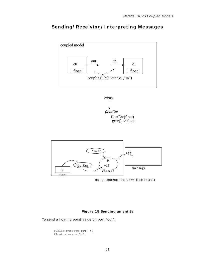
Sending/Receiving/Interpreting Messages
inoutc1c0
coupled model
coupling: (c0,”out”,c1,”in”)
float float
entity
floatEntfloatEnt(float)getv() -> float
f loat
f loa tEnt va l
p
con ten tm e s s a g e
“ou t”
make_conten t (“ou t” ,new f loa tEnt (v ) )
v
a d d
Figure 15 Sending an entity
To send a floating point value on port “out”:
public message out( ){ float store = 5.5;
Chapter 4
52
message m = new message(); content con = makeContent("out", new floatEnt(store)); m.add(con); return m; }
floatEnt
val
p
content
message
if (message_on_port(x,"in",i))
floatv
x.get_val_on_port("in",i);
“in”
x cast
getv
Figure 16 Receiving an entity
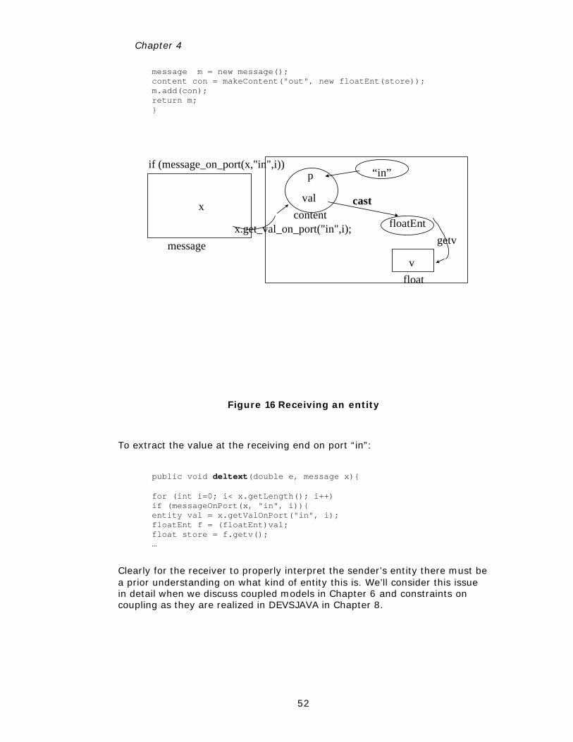
To extract the value at the receiving end on port “in”:
public void deltext(double e, message x){ for (int i=0; i< x.getLength(); i++) if (messageOnPort(x, "in", i)){ entity val = x.getValOnPort("in", i); floatEnt f = (floatEnt)val; float store = f.getv(); …
Clearly for the receiver to properly interpret the sender’s entity there must be a prior understanding on what kind of entity this is. We’ll consider this issue in detail when we discuss coupled models in Chapter 6 and constraints on coupling as they are realized in DEVSJAVA in Chapter 8.
Parallel DEVS Coupled Models
53
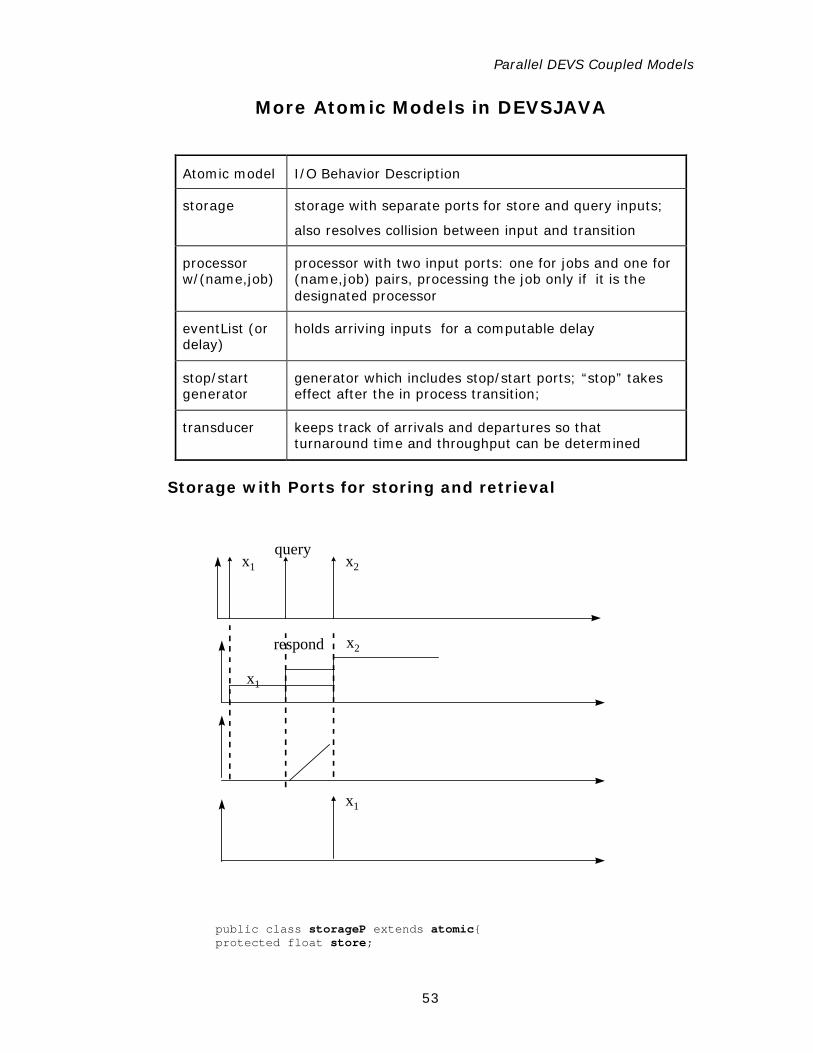
More Atomic Models in DEVSJAVA
Atomic model I/O Behavior Description
storage storage with separate ports for store and query inputs;
also resolves collision between input and transition
processor w/(name,job)
processor with two input ports: one for jobs and one for (name,job) pairs, processing the job only if it is the designated processor
eventList (or delay)
holds arriving inputs for a computable delay
stop/start generator
generator which includes stop/start ports; “stop” takes effect after the in process transition;
transducer keeps track of arrivals and departures so that turnaround time and throughput can be determined
Storage with Ports for storing and retrieval
x1
respond
x1
queryx2x1
x2
public class storageP extends atomic{ protected float store;
Chapter 4
54
protected double response_time; public storageP(String name, double Response_time){ super(name); addInport("query"); phases.add("respond”); response_time = Response_time; } public void initialize(){ phase = “passive”"; sigma = INFINITY; store = 0; response_time = 500; super.initialize(); } public void deltext(double e, message x){ Continue(e); if (phaseIs(“passive”")){ for (int i=0; i< x.getLength(); i++) if (messageOnPort(x,"in",i)){ entity val = x.getValOnPort("in", i); floatEnt f = (floatEnt)val; store = f.getv(); } for (int i=0; i< x.getLength(); i++) if (messageOnPort(x, "query", i)) holdIn("respond", response_time); } } public void deltint( ){ passivate(); } public void deltcon(double e, message x){ //inherit from atomic deltint(); deltext(0,x); } public message out( ){ message m = new message(); if (phaseIs("respond")){ content con = makeContent("out", new floatEnt(store)); m.add(con); return m; }}
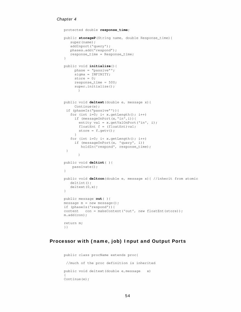
Processor with (name, job) Input and Output Ports
public class procName extends proc{ //much of the proc definition is inherited public void deltext(double e,message x) { Continue(e);
Parallel DEVS Coupled Models
55
for (int i=0; i< x.getLength();i++) if (messageOnPort(x,"inName",i)) { entity ent = x.getValOnPort("inName",i); pair pr = (pair )ent; entity en = pr.getKey(); if (this.eq(en)) // eq checks equality of names { job = pr.getValue(); holdIn("busy",processing_time); } } } public message out( ) { message m = new message(); if (phaseIs("busy")) { con = makeContent("outName",new pair(name,job)); m.add(con); } return m; } }
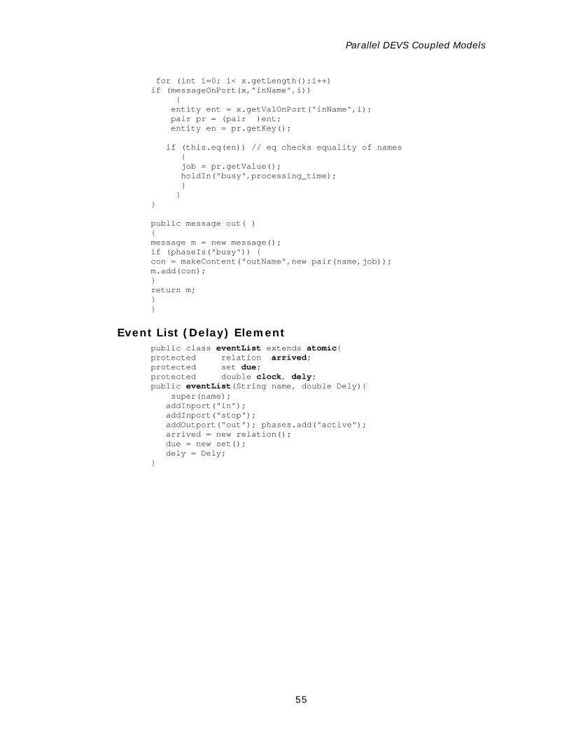
Event List (Delay) Element public class eventList extends atomic{ protected relation arrived; protected set due; protected double clock, dely; public eventList(String name, double Dely){ super(name); addInport("in"); addInport("stop"); addOutport("out"); phases.add("active"); arrived = new relation(); due = new set(); dely = Dely; }
Chapter 4
56
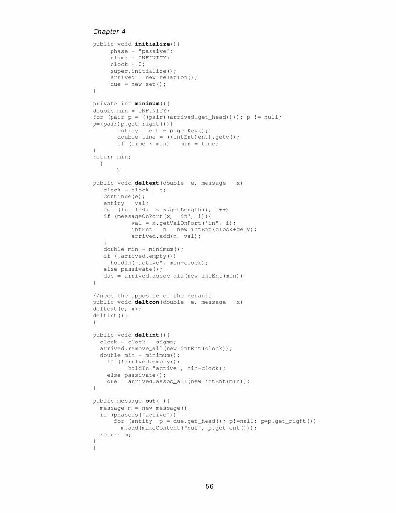
public void initialize(){ phase = "passive"; sigma = INFINITY; clock = 0; super.initialize(); arrived = new relation(); due = new set(); } private int minimum(){ double min = INFINITY; for (pair p = ((pair)(arrived.get_head())); p != null; p=(pair)p.get_right()){ entity ent = p.getKey(); double time = ((intEnt)ent).getv(); if (time < min) min = time; } return min; } } public void deltext(double e, message x){ clock = clock + e; Continue(e); entity val; for (int i=0; i< x.getLength(); i++) if (messageOnPort(x, "in", i)){ val = x.getValOnPort("in", i); intEnt n = new intEnt(clock+dely); arrived.add(n, val); } double min = minimum(); if (!arrived.empty()) holdIn("active", min-clock); else passivate(); due = arrived.assoc_all(new intEnt(min)); } //need the opposite of the default public void deltcon(double e, message x){ deltext(e, x); deltint(); } public void deltint(){ clock = clock + sigma; arrived.remove_all(new intEnt(clock)); double min = minimum(); if (!arrived.empty()) holdIn("active", min-clock); else passivate(); due = arrived.assoc_all(new intEnt(min)); } public message out( ){ message m = new message(); if (phaseIs("active")) for (entity p = due.get_head(); p!=null; p=p.get_right()) m.add(makeContent("out", p.get_ent())); return m; } }
Parallel DEVS Coupled Models
57
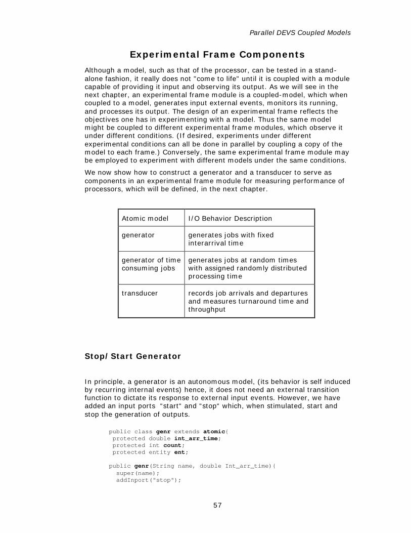
Experimental Frame Components
Although a model, such as that of the processor, can be tested in a stand-alone fashion, it really does not "come to life" until it is coupled with a module capable of providing it input and observing its output. As we will see in the next chapter, an experimental frame module is a coupled-model, which when coupled to a model, generates input external events, monitors its running, and processes its output. The design of an experimental frame reflects the objectives one has in experimenting with a model. Thus the same model might be coupled to different experimental frame modules, which observe it under different conditions. (If desired, experiments under different experimental conditions can all be done in parallel by coupling a copy of the model to each frame.) Conversely, the same experimental frame module may be employed to experiment with different models under the same conditions.
We now show how to construct a generator and a transducer to serve as components in an experimental frame module for measuring performance of processors, which will be defined, in the next chapter.
Atomic model I/O Behavior Description
generator generates jobs with fixed interarrival time
generator of time consuming jobs
generates jobs at random times with assigned randomly distributed processing time
transducer records job arrivals and departures and measures turnaround time and throughput
Stop/Start Generator
In principle, a generator is an autonomous model, (its behavior is self induced by recurring internal events) hence, it does not need an external transition function to dictate its response to external input events. However, we have added an input ports “start“ and “stop“ which, when stimulated, start and stop the generation of outputs.
public class genr extends atomic{ protected double int_arr_time; protected int count; protected entity ent; public genr(String name, double Int_arr_time){ super(name); addInport("stop");
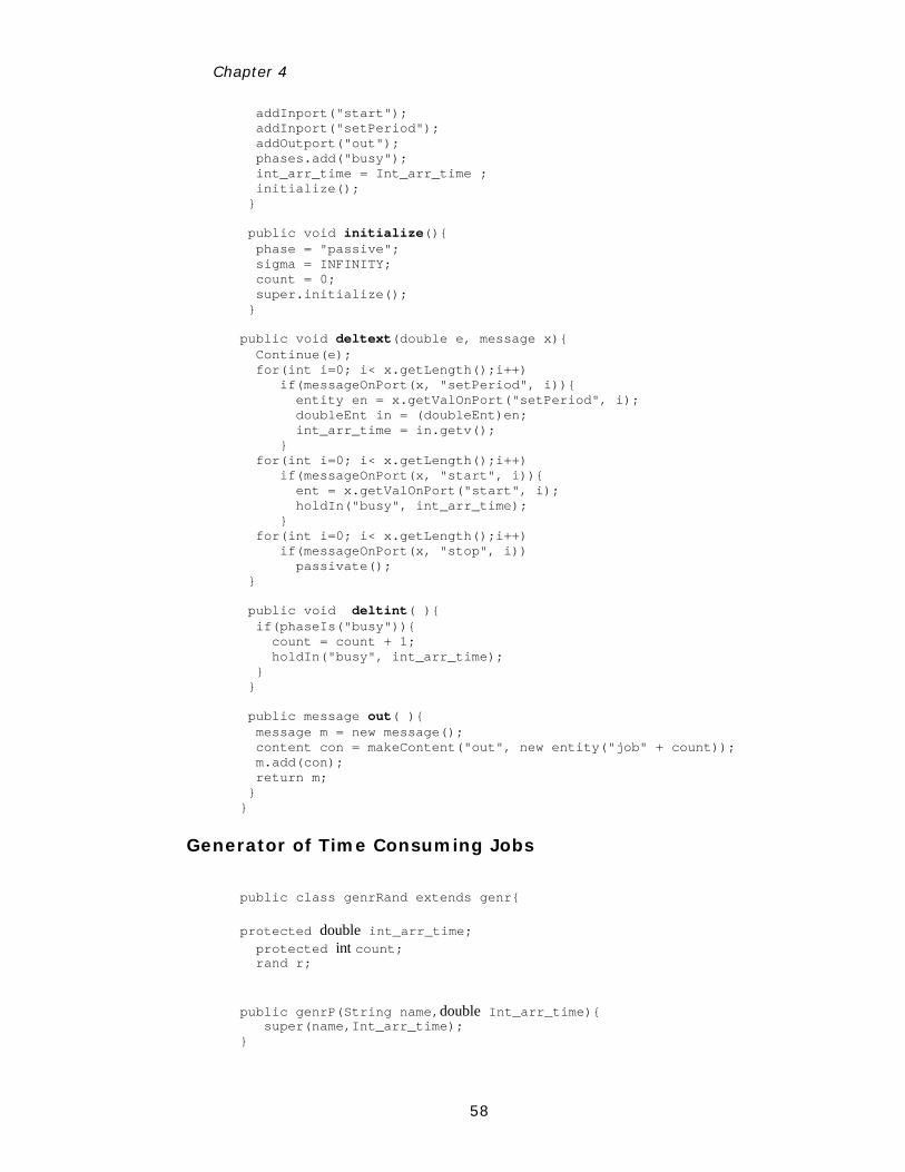
Chapter 4
58
addInport("start"); addInport("setPeriod"); addOutport("out"); phases.add("busy"); int_arr_time = Int_arr_time ; initialize(); } public void initialize(){ phase = "passive"; sigma = INFINITY; count = 0; super.initialize(); } public void deltext(double e, message x){ Continue(e); for(int i=0; i< x.getLength();i++) if(messageOnPort(x, "setPeriod", i)){ entity en = x.getValOnPort("setPeriod", i); doubleEnt in = (doubleEnt)en; int_arr_time = in.getv(); } for(int i=0; i< x.getLength();i++) if(messageOnPort(x, "start", i)){ ent = x.getValOnPort("start", i); holdIn("busy", int_arr_time); } for(int i=0; i< x.getLength();i++) if(messageOnPort(x, "stop", i)) passivate(); } public void deltint( ){ if(phaseIs("busy")){ count = count + 1; holdIn("busy", int_arr_time); } } public message out( ){ message m = new message(); content con = makeContent("out", new entity("job" + count)); m.add(con); return m; } }
Generator of Time Consuming Jobs
public class genrRand extends genr{ protected double int_arr_time; protected int count; rand r; public genrP(String name,double Int_arr_time){ super(name,Int_arr_time); }
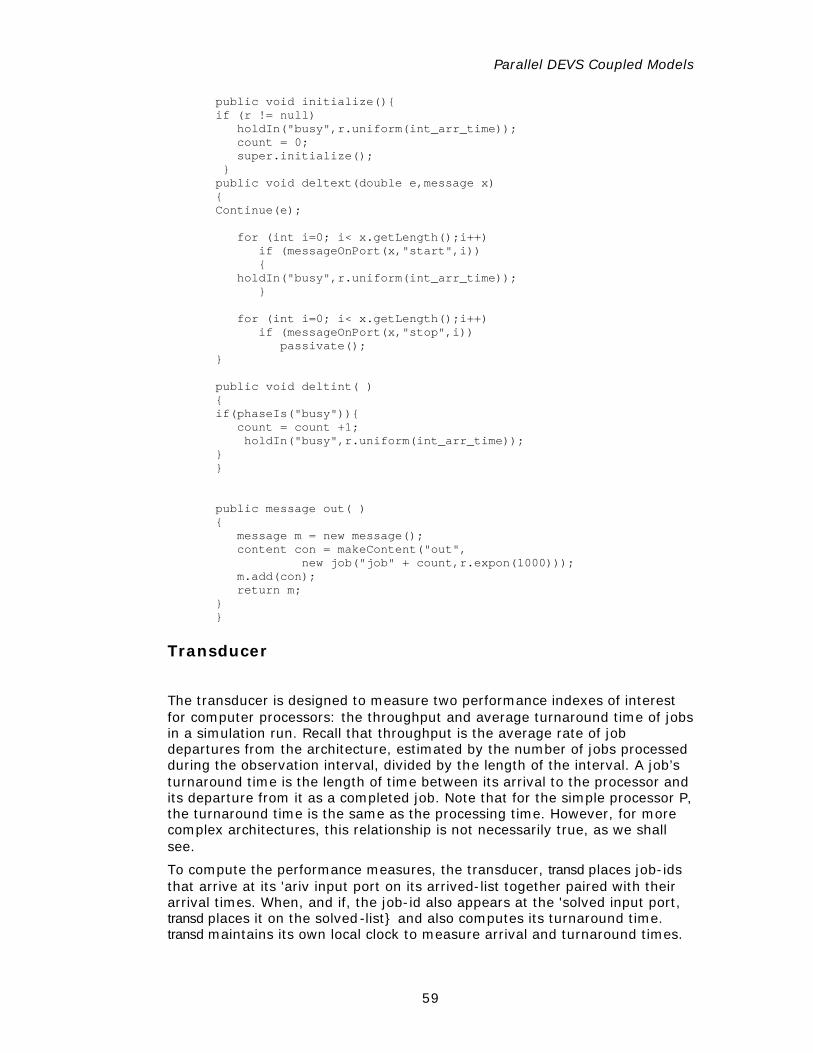
Parallel DEVS Coupled Models
59
public void initialize(){ if (r != null) holdIn("busy",r.uniform(int_arr_time)); count = 0; super.initialize(); } public void deltext(double e,message x) { Continue(e); for (int i=0; i< x.getLength();i++) if (messageOnPort(x,"start",i)) { holdIn("busy",r.uniform(int_arr_time)); } for (int i=0; i< x.getLength();i++) if (messageOnPort(x,"stop",i)) passivate(); } public void deltint( ) { if(phaseIs("busy")){ count = count +1; holdIn("busy",r.uniform(int_arr_time)); } } public message out( ) { message m = new message(); content con = makeContent("out", new job("job" + count,r.expon(1000))); m.add(con); return m; } }
Transducer
The transducer is designed to measure two performance indexes of interest for computer processors: the throughput and average turnaround time of jobs in a simulation run. Recall that throughput is the average rate of job departures from the architecture, estimated by the number of jobs processed during the observation interval, divided by the length of the interval. A job’s turnaround time is the length of time between its arrival to the processor and its departure from it as a completed job. Note that for the simple processor P, the turnaround time is the same as the processing time. However, for more complex architectures, this relationship is not necessarily true, as we shall see.
To compute the performance measures, the transducer, transd places job-ids that arrive at its 'ariv input port on its arrived-list together paired with their arrival times. When, and if, the job-id also appears at the 'solved input port, transd places it on the solved-list} and also computes its turnaround time. transd maintains its own local clock to measure arrival and turnaround times.
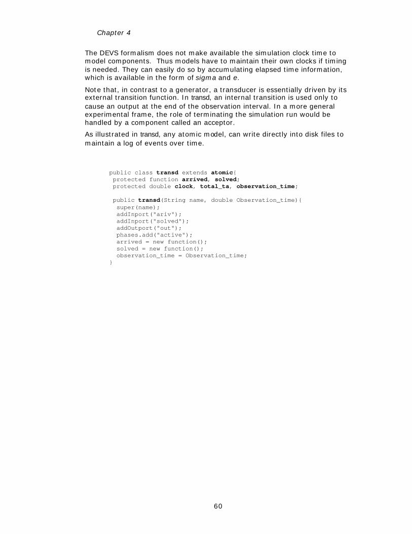
Chapter 4
60
The DEVS formalism does not make available the simulation clock time to model components. Thus models have to maintain their own clocks if timing is needed. They can easily do so by accumulating elapsed time information, which is available in the form of sigma and e.
Note that, in contrast to a generator, a transducer is essentially driven by its external transition function. In transd, an internal transition is used only to cause an output at the end of the observation interval. In a more general experimental frame, the role of terminating the simulation run would be handled by a component called an acceptor.
As illustrated in transd, any atomic model, can write directly into disk files to maintain a log of events over time.
public class transd extends atomic{ protected function arrived, solved; protected double clock, total_ta, observation_time; public transd(String name, double Observation_time){ super(name); addInport("ariv"); addInport("solved"); addOutport("out"); phases.add("active"); arrived = new function(); solved = new function(); observation_time = Observation_time; }
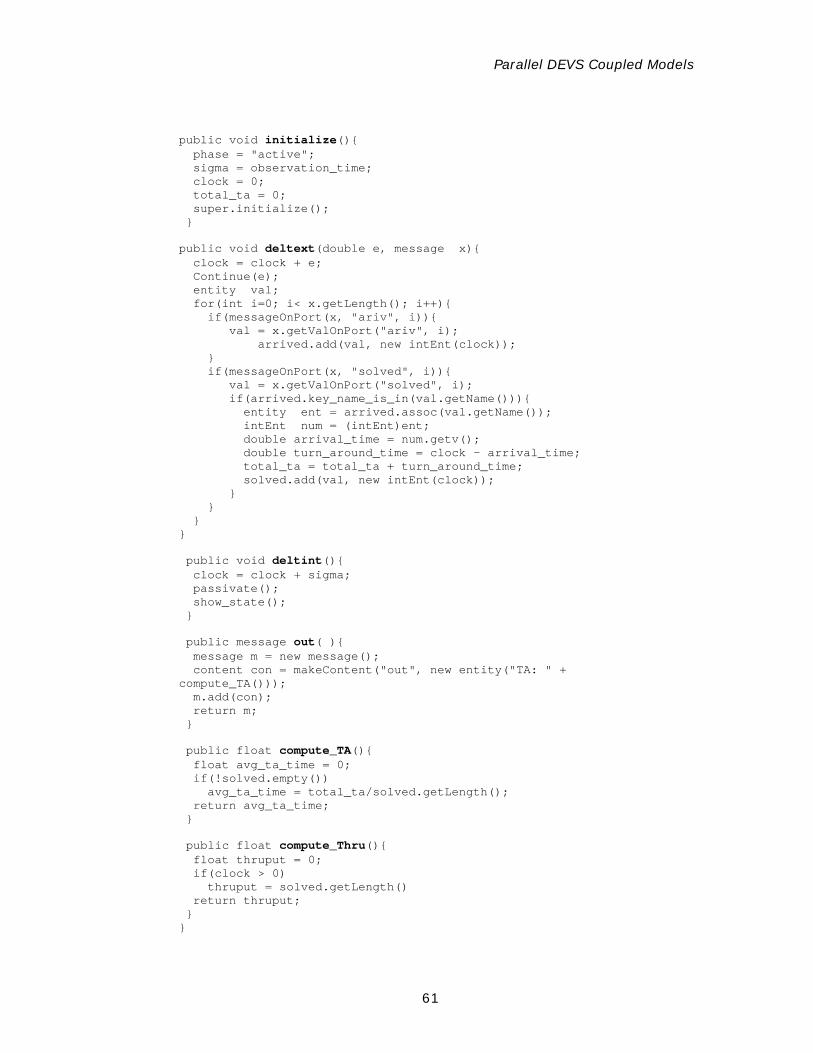
Parallel DEVS Coupled Models
61
public void initialize(){ phase = "active"; sigma = observation_time; clock = 0; total_ta = 0; super.initialize(); } public void deltext(double e, message x){ clock = clock + e; Continue(e); entity val; for(int i=0; i< x.getLength(); i++){ if(messageOnPort(x, "ariv", i)){ val = x.getValOnPort("ariv", i); arrived.add(val, new intEnt(clock)); } if(messageOnPort(x, "solved", i)){ val = x.getValOnPort("solved", i); if(arrived.key_name_is_in(val.getName())){ entity ent = arrived.assoc(val.getName()); intEnt num = (intEnt)ent; double arrival_time = num.getv(); double turn_around_time = clock - arrival_time; total_ta = total_ta + turn_around_time; solved.add(val, new intEnt(clock)); } } } } public void deltint(){ clock = clock + sigma; passivate(); show_state(); } public message out( ){ message m = new message(); content con = makeContent("out", new entity("TA: " + compute_TA())); m.add(con); return m; } public float compute_TA(){ float avg_ta_time = 0; if(!solved.empty()) avg_ta_time = total_ta/solved.getLength(); return avg_ta_time; } public float compute_Thru(){ float thruput = 0; if(clock > 0) thruput = solved.getLength() return thruput; } }
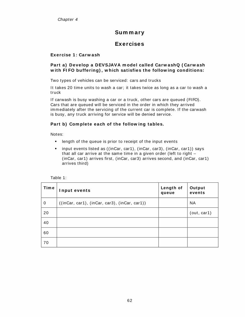
Chapter 4
62
Summary
Exercises
Exercise 1: Carwash
Part a) Develop a DEVSJAVA model called CarwashQ (Carwash with FIFO buffering), which satisfies the following conditions:
Two types of vehicles can be serviced: cars and trucks
It takes 20 time units to wash a car; it takes twice as long as a car to wash a truck
If carwash is busy washing a car or a truck, other cars are queued (FIFO). Cars that are queued will be serviced in the order in which they arrived immediately after the servicing of the current car is complete. If the carwash is busy, any truck arriving for service will be denied service.
Part b) Complete each of the following tables.
Notes:
§ length of the queue is prior to receipt of the input events
§ input events listed as ((inCar, car1), (inCar, car3), (inCar, car1)) says that all car arrive at the same time in a given order (left to right – (inCar, car1) arrives first, (inCar, car3) arrives second, and (inCar, car1) arrives third)
Table 1:
Time Input events
Length of queue
Output events
0 ((inCar, car1), (inCar, car3), (inCar, car1)) NA
20 (out, car1)
40
60
70
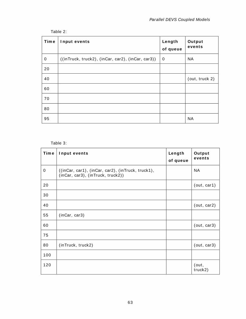
Parallel DEVS Coupled Models
63
Table 2:
Time Input events Length
of queue
Output events
0 ((inTruck, truck2), (inCar, car2), (inCar, car3)) 0 NA
20
40 (out, truck 2)
60
70
80
95 NA
Table 3:
Time Input events Length
of queue
Output events
0 ((inCar, car1), (inCar, car2), (inTruck, truck1), (inCar, car3), (inTruck, truck2))
NA
20 (out, car1)
30
40 (out, car2)
55 (inCar, car3)
60 (out, car3)
75
80 (inTruck, truck2) (out, car3)
100
120 (out, truck2)
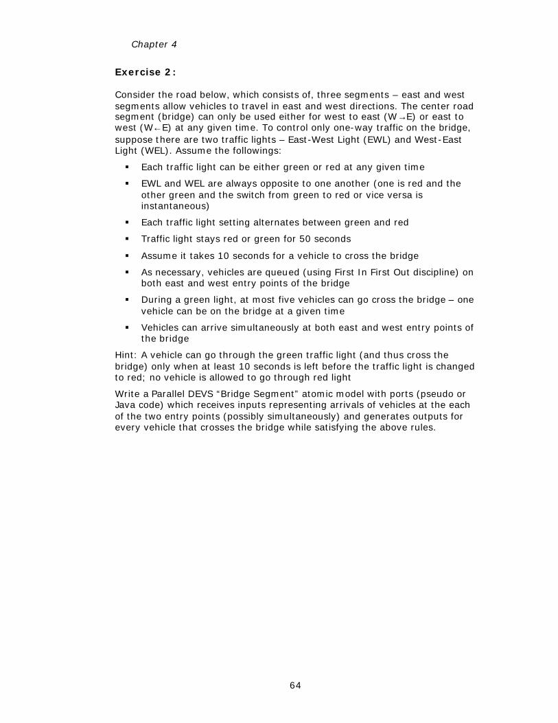
Chapter 4
64
Exercise 2:
Consider the road below, which consists of, three segments – east and west segments allow vehicles to travel in east and west directions. The center road segment (bridge) can only be used either for west to east (W→E) or east to west (W←E) at any given time. To control only one-way traffic on the bridge, suppose there are two traffic lights – East-West Light (EWL) and West-East Light (WEL). Assume the followings:
§ Each traffic light can be either green or red at any given time
§ EWL and WEL are always opposite to one another (one is red and the other green and the switch from green to red or vice versa is instantaneous)
§ Each traffic light setting alternates between green and red
§ Traffic light stays red or green for 50 seconds
§ Assume it takes 10 seconds for a vehicle to cross the bridge
§ As necessary, vehicles are queued (using First In First Out discipline) on both east and west entry points of the bridge
§ During a green light, at most five vehicles can go cross the bridge – one vehicle can be on the bridge at a given time
§ Vehicles can arrive simultaneously at both east and west entry points of the bridge
Hint: A vehicle can go through the green traffic light (and thus cross the bridge) only when at least 10 seconds is left before the traffic light is changed to red; no vehicle is allowed to go through red light
Write a Parallel DEVS “Bridge Segment” atomic model with ports (pseudo or Java code) which receives inputs representing arrivals of vehicles at the each of the two entry points (possibly simultaneously) and generates outputs for every vehicle that crosses the bridge while satisfying the above rules.
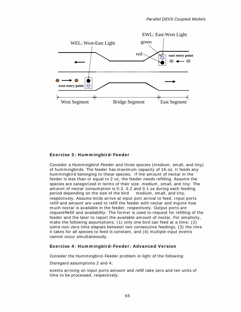
Parallel DEVS Coupled Models
65
EWL: East-West Light
east entry point
west entry point
WEL: West-East Light green
red
West Segment East SegmentBridge Segment
Exercise 3: Hummingbird-Feeder
Consider a Hummingbird-Feeder and three species (medium, small, and tiny) of hummingbirds. The feeder has maximum capacity of 16 oz. It feeds any hummingbird belonging to these species. If the amount of nectar in the feeder is less than or equal to 2 oz, the feeder needs refilling. Assume the species are categorized in terms of their size: medium, small, and tiny. The amount of nectar consumption is 0.3, 0.2 and 0.1 oz during each feeding period depending on the size of the bird medium, small, and tiny, respectively. Assume birds arrive at input port arrival to feed. Input ports refill and amount are used to refill the feeder with nectar and inquire how much nectar is available in the feeder, respectively. Output ports are requestRefill and availability. The former is used to request for refilling of the feeder and the later to report the available amount of nectar. For simplicity, make the following assumptions: (1) only one bird can feed at a time; (2) some non-zero time elapses between two consecutive feedings, (3) the time it takes for all species to feed is constant, and (4) multiple input events cannot occur simultaneously.
Exercise 4: Hummingbird-Feeder: Advanced Version
Consider the Hummingbird-Feeder problem in light of the following:
Disregard assumptions 2 and 4;
events arriving on input ports amount and refill take zero and ten units of time to be processed, respectively;
Chapter 4
66
constant consumption rate for each type of bird − each uninterrupted round of feeding takes 15 units of time;
while a bird is feeding, it can be interrupted by another bird. Assume the bird that gets interrupted will not return to complete it’s feeding, but can always begin a new round of feeding!
Recall from problem statement below that it takes the same amount of time for each type of bird (i.e., tiny, small, medium) to fully consume its maximum allowed nectar consumption (i.e., 0.1, 0.2, and 0.3 oz respectively) in each feeding session. Implement the revised hummingbird-feeder in DEVSJAVA. Devise representative input sequences in order to ensure correctness of the model and its implementation.
Solution
Exercise 4: Hummingbird-Feeder: Advanced Version
Additional assumptions:
Hummingbird-feeder ignores external events if it is not in phase “passive”
Duration period assignments for Feed, refill, and query are all finite and at least equal to one unit of time
When available nectar is to become less than 2.0 oz, refill order is issued. However, note that more than 2 oz of nectar must be available before a bird can feed.
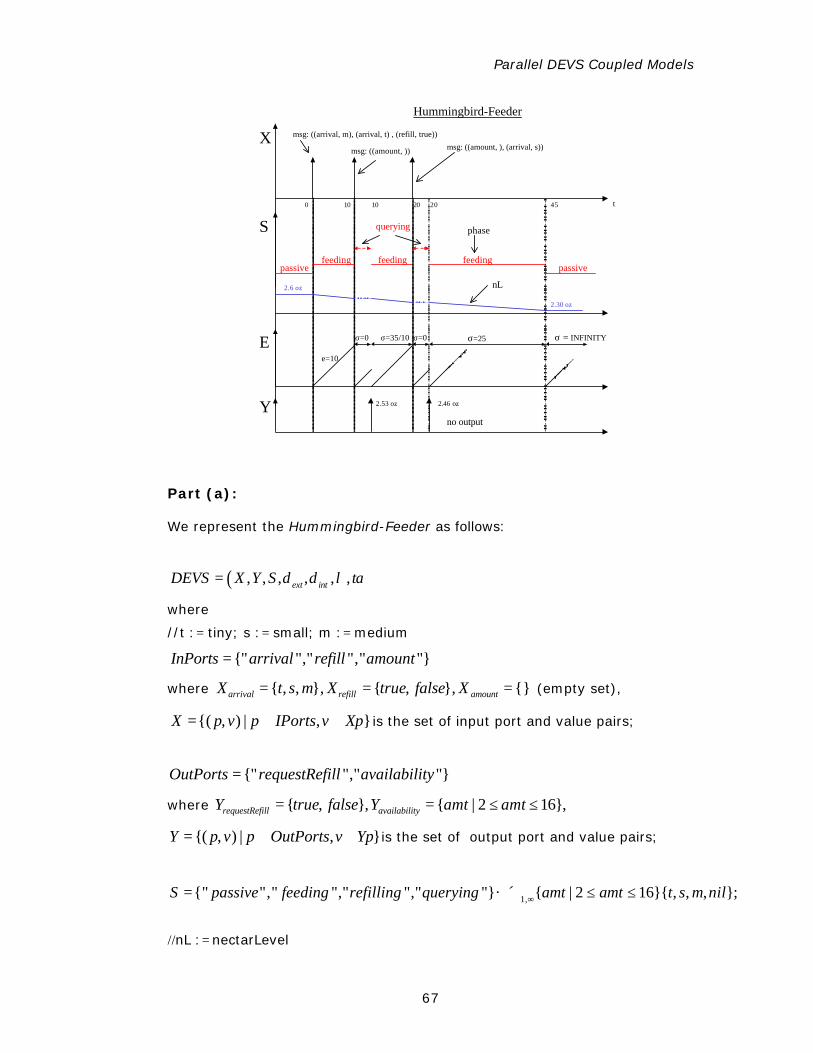
Parallel DEVS Coupled Models
67
X
0
S
t
E
Y
Hummingbird-Feeder
10
e=10
σ=25
msg: ((arrival, m), (arrival, t) , (refill, true))
passive
σ=35/10
feeding
msg: ((amount, ))
20
feeding
no output
10
querying
msg: ((amount, ), (arrival, s))
45
feedingpassive
2.30 oz
2.53 oz 2.46 oz
2.6 oz nL
20
σ = INFINITY
phase
σ=0 σ=0
Part (a):
We represent the Hummingbird-Feeder as follows:
( ), , , , , ,ext intDEVS X Y S taδ δ λ=
where
//t := tiny; s := small; m := medium
{" "," "," "}InPorts arrival refill amount=
where { , , }, { , }, {}arrival refill amountX t s m X true false X= = = (empty set),
{( , ) | , }X p v p IPorts v Xp= ∈ ∈ is the set of input port and value pairs;
{" "," "}OutPorts requestRefill availability=
where { , }, { | 2 16},requestRefill availabilityY true false Y amt amt= = ≤ ≤
{( , ) | , }Y p v p OutPorts v Yp= ∈ ∈ is the set of output port and value pairs;
1,{" "," "," "," "} { | 2 16}{ , , , };S passive feeding refilling querying amt amt t s m nil× ℜ +∞= ≤ ≤
//nL := nectarLevel
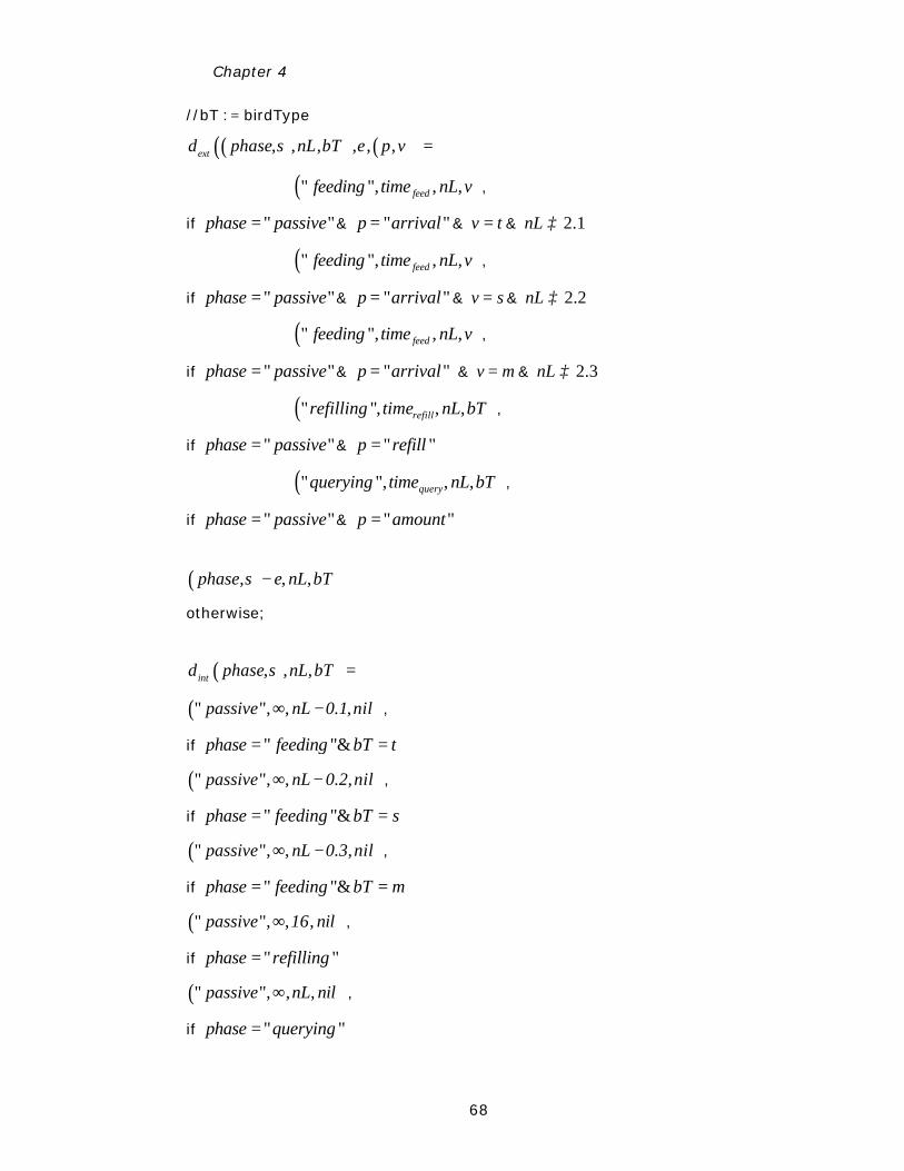
Chapter 4
68
//bT := birdType
( ) ( )( ), , , , , ,ext phase nL bT e p vδ σ =
( )" ", , ,feedfeeding time nL v ,
if " "phase passive= & " "p arrival= & v t= & 2.1nL ≥
( )" ", , ,feedfeeding time nL v ,
if " "phase passive= & " "p arrival= & v s= & 2.2nL ≥
( )" ", , ,feedfeeding time nL v ,
if " "phase passive= & " "p arrival= & v m= & 2.3nL ≥
( )" ", , ,refillrefilling time nL bT ,
if " "phase passive= & " "p refill=
( )" ", , ,queryquerying time nL bT ,
if " "phase passive= & " "p amount=
( ), , ,phase e nL bTσ −
otherwise;
( ), , ,int phase nL bTδ σ =
( )" ", , ,passive nL 0.1 nil∞ − ,
if " "&phase feeding bT t= =
( )" ", , ,passive nL 0.2 nil∞ − ,
if " "&phase feeding bT s= =
( )" ", , ,passive nL 0.3 nil∞ − ,
if " "&phase feeding bT m= =
( )" ", , ,passive 16 nil∞ ,
if " "phase refilling=
( )" ", , ,passive nL nil∞ ,
if " "phase querying=
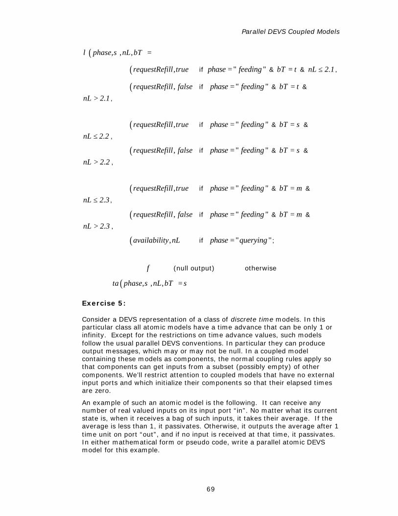
Parallel DEVS Coupled Models
69
( ), , ,phase nL bTλ σ =
( ),requestRefill true if " "phase feeding= & bT t= & nL 2.1≤ ,
( ),requestRefill false if " "phase feeding= & bT t= &
nL 2.1> ,
( ),requestRefill true if " "phase feeding= & bT s= &
nL 2.2≤ ,
( ),requestRefill false if " "phase feeding= & bT s= &
nL 2.2> ,
( ),requestRefill true if " "phase feeding= & bT m= &
nL 2.3≤ ,
( ),requestRefill false if " "phase feeding= & bT m= &
nL 2.3> ,
( ),availability nL if " "phase querying= ;
φ (null output) otherwise
( ), , ,ta phase nL bTσ σ=
Exercise 5:
Consider a DEVS representation of a class of discrete time models. In this particular class all atomic models have a time advance that can be only 1 or infinity. Except for the restrictions on time advance values, such models follow the usual parallel DEVS conventions. In particular they can produce output messages, which may or may not be null. In a coupled model containing these models as components, the normal coupling rules apply so that components can get inputs from a subset (possibly empty) of other components. We’ll restrict attention to coupled models that have no external input ports and which initialize their components so that their elapsed times are zero.
An example of such an atomic model is the following. It can receive any number of real valued inputs on its input port “in”. No matter what its current state is, when it receives a bag of such inputs, it takes their average. If the average is less than 1, it passivates. Otherwise, it outputs the average after 1 time unit on port “out”, and if no input is received at that time, it passivates. In either mathematical form or pseudo code, write a parallel atomic DEVS model for this example.
Chapter 4
70
Using the standard Parallel DEVS simulation protocol, describe the exact conditions under which the internal, external and confluent transition functions of the components are applied in a simulations of coupled models with components described in a).
Consider coupled models of components of the discrete time class described above (of which those in a) are special cases). Assume the number of components is very large and the maximum number of influences of any component (the possible receivers of its output) is very much smaller. Develop an optimization of the standard Parallel DEVS simulation protocol that allows the coordinator to use its knowledge of the restricted time advances and the model coupling information to reduce the number of messages it exchanges with the simulators of the components. Your algorithms for coordinator and simulator can be given in any convenient form. Explain where your version provides the savings in messages in comparison to the standard protocol.
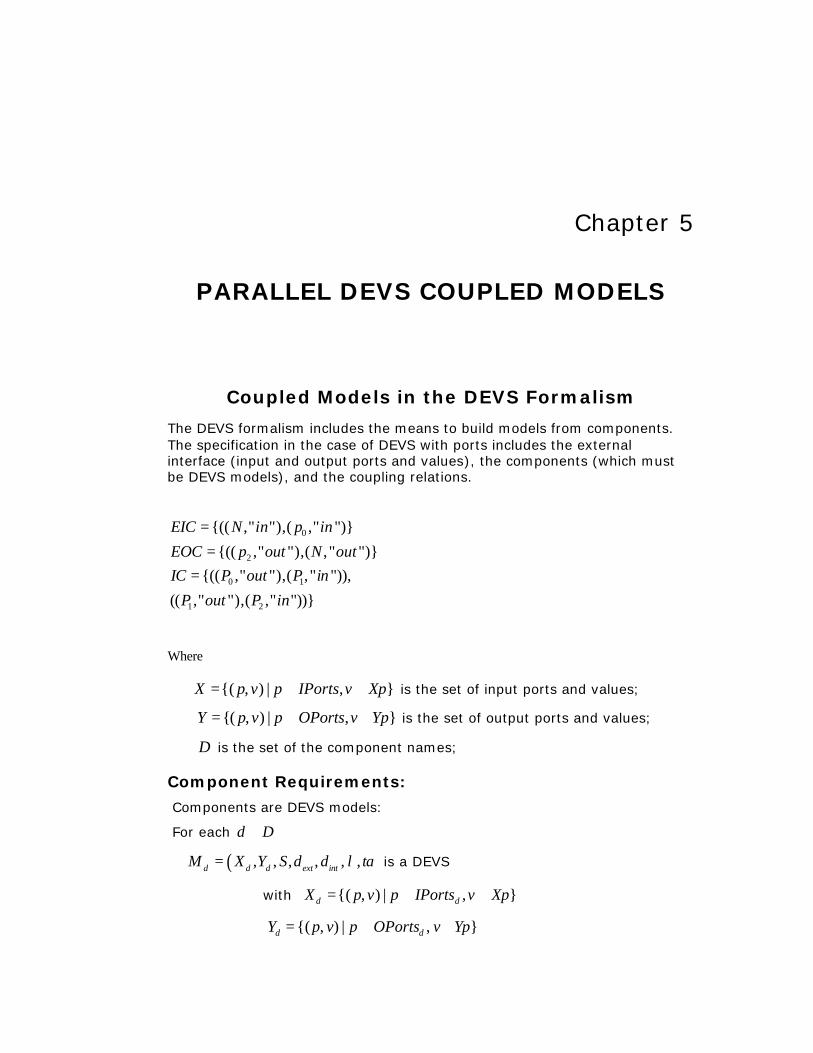
Chapter 5
PARALLEL DEVS COUPLED MODELS
Coupled Models in the DEVS Formalism
The DEVS formalism includes the means to build models from components. The specification in the case of DEVS with ports includes the external interface (input and output ports and values), the components (which must be DEVS models), and the coupling relations.
0
2
0 1
1 2
{(( ," "),( ," ")}
{(( ," "),( ," ")}{(( ," "),( ," ")),
(( ," "),( ," "))}
EIC N in p in
EOC p out N outIC P out P in
P out P in
=
==
Where
{( , ) | , }X p v p IPorts v Xp= ∈ ∈ is the set of input ports and values;
{( , ) | , }Y p v p OPorts v Yp= ∈ ∈ is the set of output ports and values;
D is the set of the component names;
Component Requirements:
Components are DEVS models:
For each d D∈
( ), , , , , ,d d d ext intM X Y S taδ δ λ= is a DEVS
with {( , ) | , }d dX p v p IPorts v Xp= ∈ ∈
{( , ) | , }d dY p v p OPorts v Yp= ∈ ∈
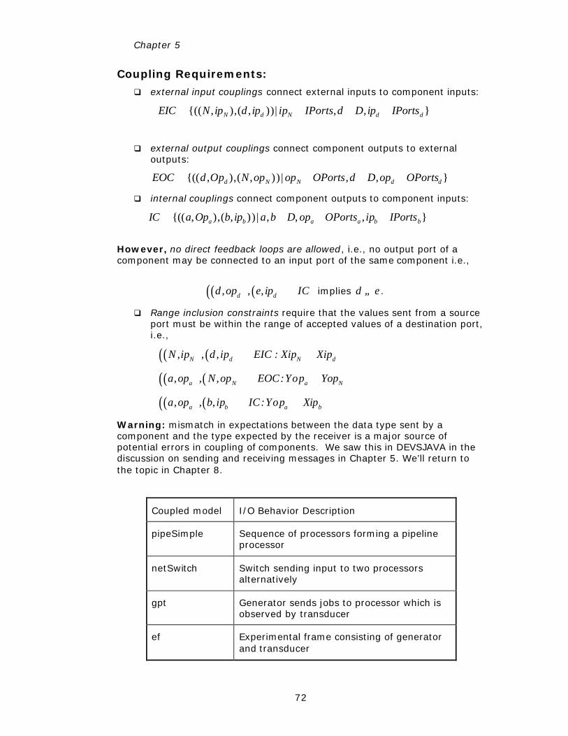
Chapter 5
72
Coupling Requirements:
q external input couplings connect external inputs to component inputs:
{(( , ),( , ))| , , }N d N d dEIC N ip d ip ip IPorts d D ip IPorts⊆ ∈ ∈ ∈
q external output couplings connect component outputs to external outputs:
{(( , ),( , )) | , , }d N N d dEOC d Op N op op OPorts d D op OPorts⊆ ∈ ∈ ∈
q internal couplings connect component outputs to component inputs:
{(( , ),( , )) | , , , }a b a a b bIC a Op b ip a b D op OPorts ip IPorts⊆ ∈ ∈ ∈
However, no direct feedback loops are allowed, i.e., no output port of a component may be connected to an input port of the same component i.e.,
( ) ( )( ), , ,d dd op e ip IC∈ implies d e≠ .
q Range inclusion constraints require that the values sent from a source port must be within the range of accepted values of a destination port, i.e.,
( ) ( )( ), , ,N d N dN ip d ip EIC : Xip Xip∀ ∈ ⊆
( ) ( )( ), , ,a N a Na op N op EOC:Yop Yop∀ ∈ ⊆
( ) ( )( ), , ,a b a ba op b ip IC:Yop Xip∀ ∈ ⊆
Warning: mismatch in expectations between the data type sent by a component and the type expected by the receiver is a major source of potential errors in coupling of components. We saw this in DEVSJAVA in the discussion on sending and receiving messages in Chapter 5. We’ll return to the topic in Chapter 8.
Coupled model I/O Behavior Description
pipeSimple Sequence of processors forming a pipeline processor
netSwitch Switch sending input to two processors alternatively
gpt Generator sends jobs to processor which is observed by transducer
ef Experimental frame consisting of generator and transducer
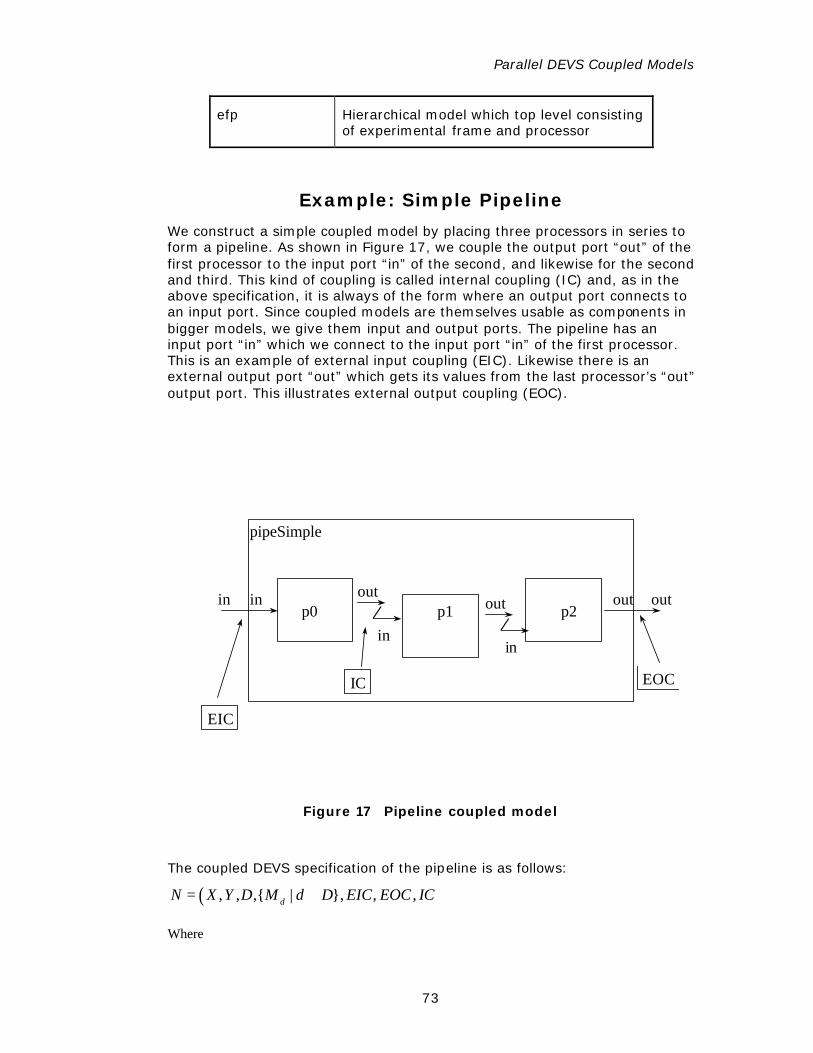
Parallel DEVS Coupled Models
73
efp Hierarchical model which top level consisting of experimental frame and processor
Example: Simple Pipeline
We construct a simple coupled model by placing three processors in series to form a pipeline. As shown in Figure 17, we couple the output port “out” of the first processor to the input port “in” of the second, and likewise for the second and third. This kind of coupling is called internal coupling (IC) and, as in the above specification, it is always of the form where an output port connects to an input port. Since coupled models are themselves usable as components in bigger models, we give them input and output ports. The pipeline has an input port “in” which we connect to the input port “in” of the first processor. This is an example of external input coupling (EIC). Likewise there is an external output port “out” which gets its values from the last processor’s “out” output port. This illustrates external output coupling (EOC).
in outoutp2p1p0
pipeSimple
in
in
out
in
out
EIC
IC EOC
Figure 17 Pipeline coupled model
The coupled DEVS specification of the pipeline is as follows:
( ), , ,{ | }, , ,dN X Y D M d D EIC EOC IC= ∈
Where
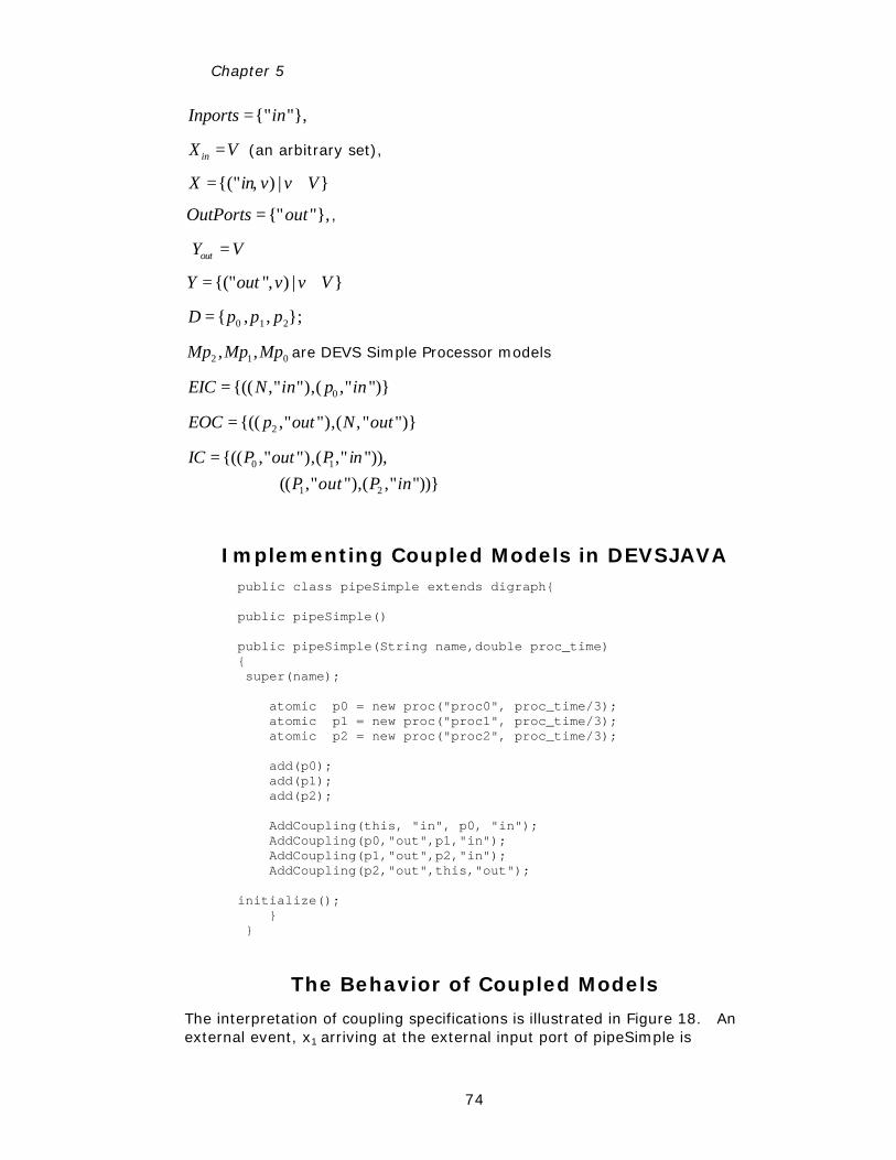
Chapter 5
74
{" "},Inports in=
inX V= (an arbitrary set),
{(" , ) | }X in v v V= ∈
{" "},OutPorts out= ,
outY V=
{(" ", ) | }Y out v v V= ∈
0 1 2{ , , };D p p p=
2 1 0, ,Mp Mp Mp are DEVS Simple Processor models
0{(( ," "),( ," ")}EIC N in p in=
2{(( ," "),( ," ")}EOC p out N out=
0 1{(( ," "),( ," ")),IC P out P in=
1 2(( ," "),( ," "))}P out P in
Implementing Coupled Models in DEVSJAVA public class pipeSimple extends digraph{ public pipeSimple() public pipeSimple(String name,double proc_time) { super(name); atomic p0 = new proc("proc0", proc_time/3); atomic p1 = new proc("proc1", proc_time/3); atomic p2 = new proc("proc2", proc_time/3); add(p0); add(p1); add(p2); AddCoupling(this, "in", p0, "in"); AddCoupling(p0,"out",p1,"in"); AddCoupling(p1,"out",p2,"in"); AddCoupling(p2,"out",this,"out"); initialize(); } }
The Behavior of Coupled Models
The interpretation of coupling specifications is illustrated in Figure 18. An external event, x1 arriving at the external input port of pipeSimple is
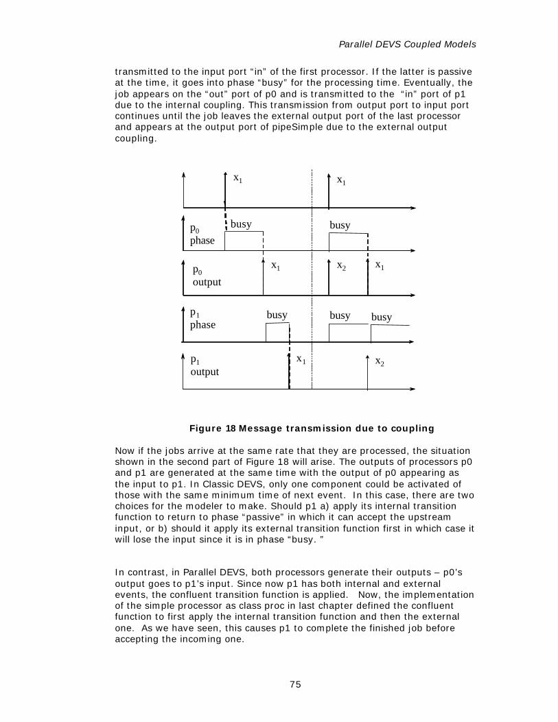
Parallel DEVS Coupled Models
75
transmitted to the input port “in” of the first processor. If the latter is passive at the time, it goes into phase “busy” for the processing time. Eventually, the job appears on the “out” port of p0 and is transmitted to the “in” port of p1 due to the internal coupling. This transmission from output port to input port continues until the job leaves the external output port of the last processor and appears at the output port of pipeSimple due to the external output coupling.
x1
busy
busy
x1
p0phase
p0output
p1phase
p1output
busy
busybusy
x2
x1
x1
x1
x2
Figure 18 Message transmission due to coupling
Now if the jobs arrive at the same rate that they are processed, the situation shown in the second part of Figure 18 will arise. The outputs of processors p0 and p1 are generated at the same time with the output of p0 appearing as the input to p1. In Classic DEVS, only one component could be activated of those with the same minimum time of next event. In this case, there are two choices for the modeler to make. Should p1 a) apply its internal transition function to return to phase “passive” in which it can accept the upstream input, or b) should it apply its external transition function first in which case it will lose the input since it is in phase “busy. ”
In contrast, in Parallel DEVS, both processors generate their outputs – p0’s output goes to p1’s input. Since now p1 has both internal and external events, the confluent transition function is applied. Now, the implementation of the simple processor as class proc in last chapter defined the confluent function to first apply the internal transition function and then the external one. As we have seen, this causes p1 to complete the finished job before accepting the incoming one.
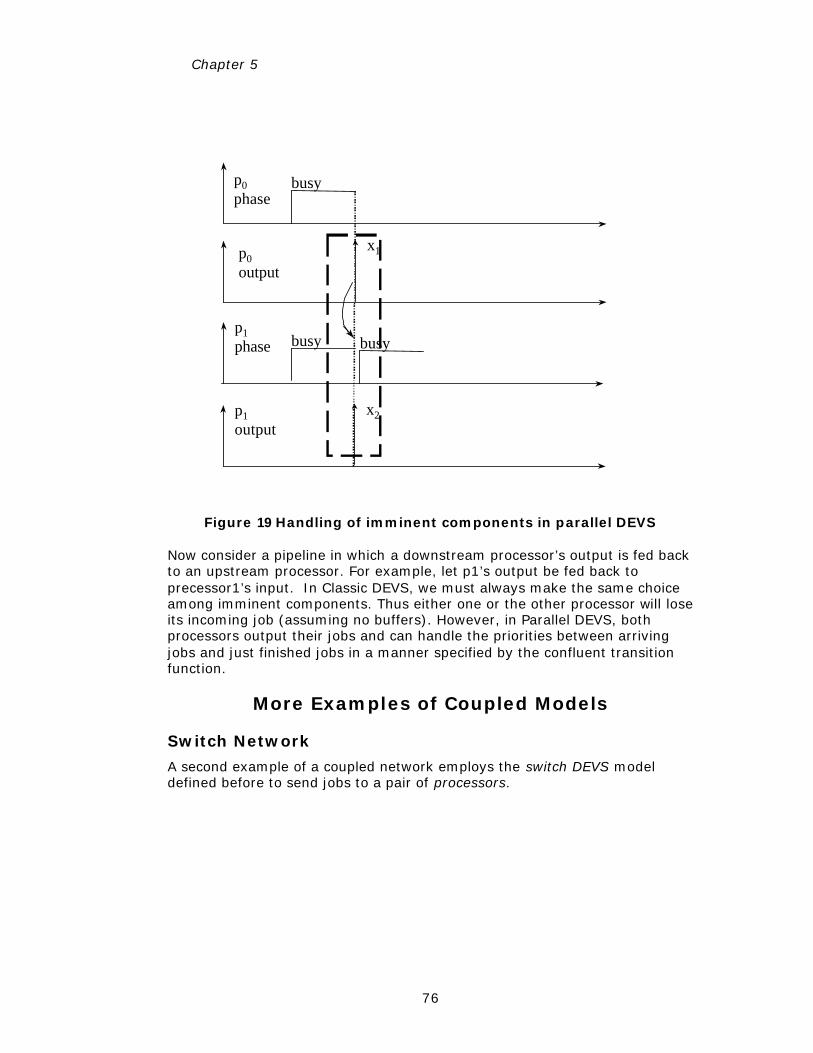
Chapter 5
76
busy
x1
busybusy
x2
p0phase
p0output
p1phase
p1output
Figure 19 Handling of imminent components in parallel DEVS
Now consider a pipeline in which a downstream processor’s output is fed back to an upstream processor. For example, let p1’s output be fed back to precessor1’s input. In Classic DEVS, we must always make the same choice among imminent components. Thus either one or the other processor will lose its incoming job (assuming no buffers). However, in Parallel DEVS, both processors output their jobs and can handle the priorities between arriving jobs and just finished jobs in a manner specified by the confluent transition function.
More Examples of Coupled Models
Switch Network
A second example of a coupled network employs the switch DEVS model defined before to send jobs to a pair of processors.
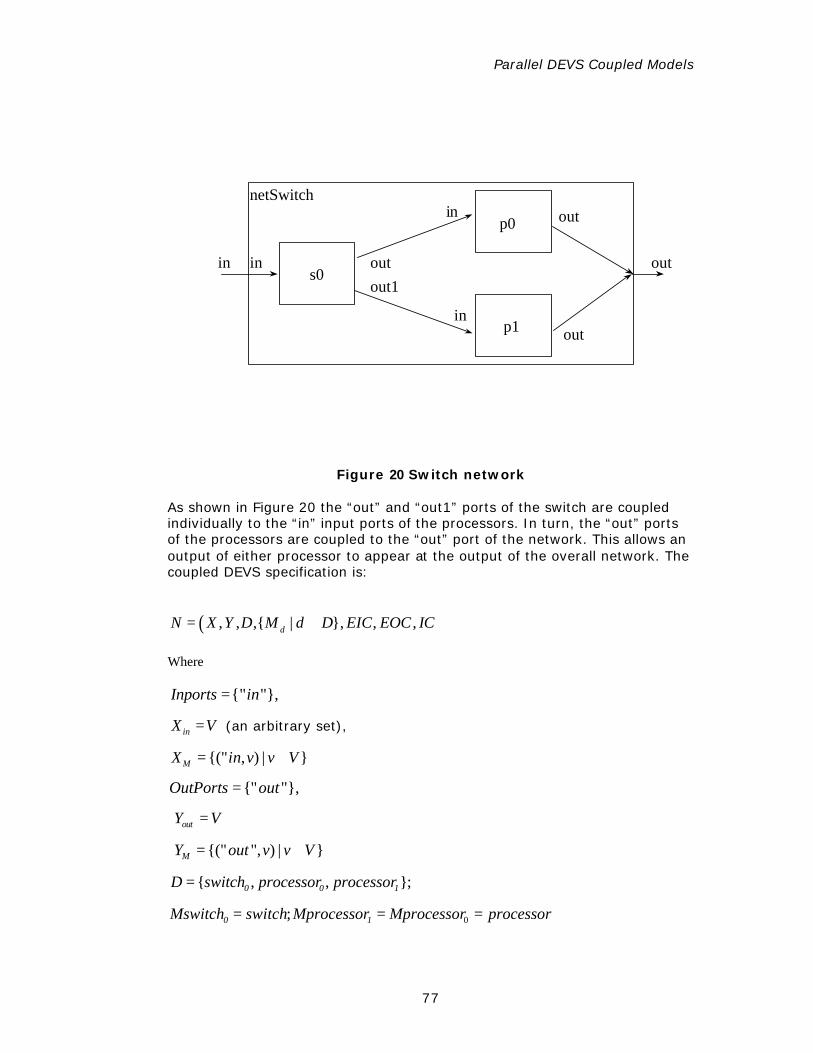
Parallel DEVS Coupled Models
77
in outs0
netSwitch
in
out
p1
p0
out
outout1
in
in
Figure 20 Switch network
As shown in Figure 20 the “out” and “out1” ports of the switch are coupled individually to the “in” input ports of the processors. In turn, the “out” ports of the processors are coupled to the “out” port of the network. This allows an output of either processor to appear at the output of the overall network. The coupled DEVS specification is:
( ), , ,{ | }, , ,dN X Y D M d D EIC EOC IC= ∈
Where
{" "},Inports in=
inX V= (an arbitrary set),
{(" , ) | }MX in v v V= ∈
{" "},OutPorts out=
outY V=
{(" ", ) | }MY out v v V= ∈
{ , , };0 0 1D switch processor processor=
0;0 1Mswitch switch Mprocessor Mprocessor processor= = =
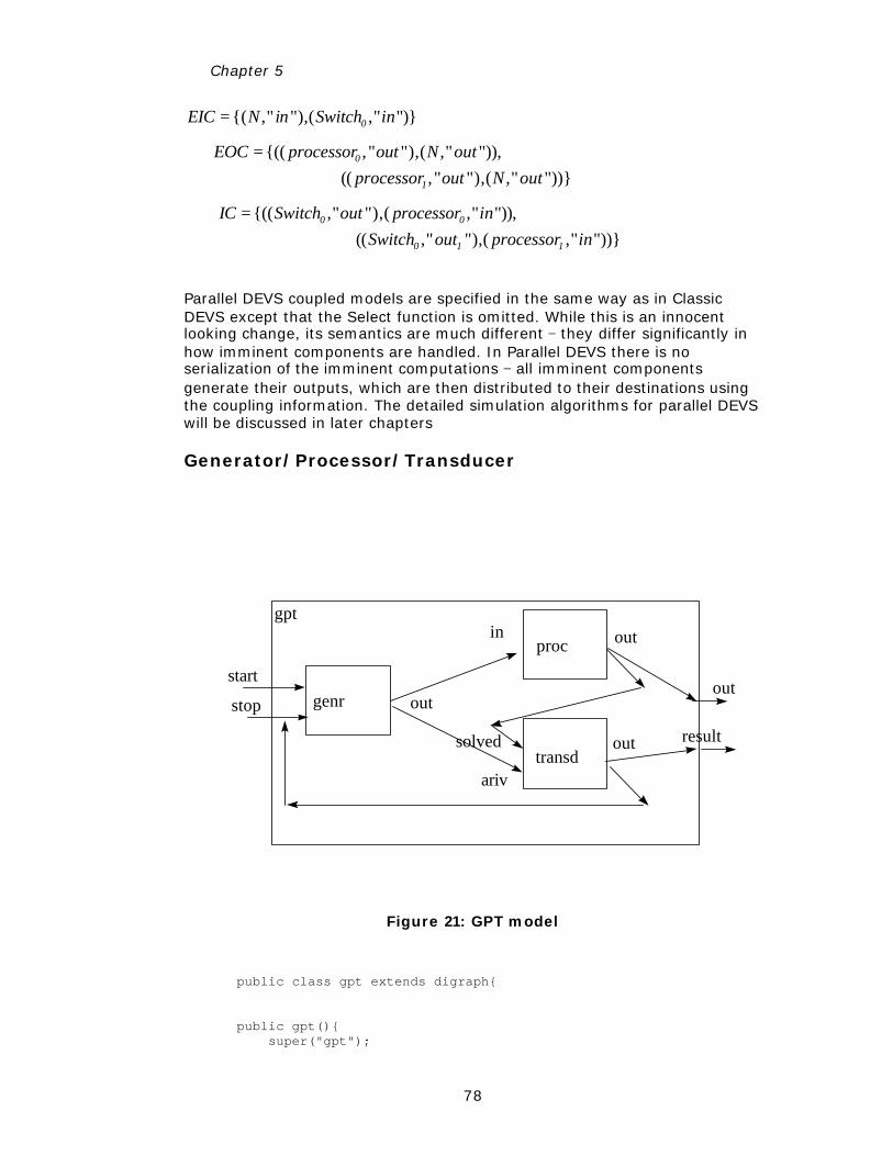
Chapter 5
78
{( ," "),( ," ")}0EIC N in Switch in=
{(( ," "),( ," ")),0EOC processor out N out=
(( ," "),( ," "))}1processor out N out
{(( ," "),( ," ")),0 0IC Switch out processor in=
(( ," "),( ," "))}0 1 1Switch out processor in
Parallel DEVS coupled models are specified in the same way as in Classic DEVS except that the Select function is omitted. While this is an innocent looking change, its semantics are much different − they differ significantly in how imminent components are handled. In Parallel DEVS there is no serialization of the imminent computations − all imminent components generate their outputs, which are then distributed to their destinations using the coupling information. The detailed simulation algorithms for parallel DEVS will be discussed in later chapters
Generator/Processor/Transducer
genr
gpt
start
transd
proc
out
out
out
out
in
ariv
solved result
stop
Figure 21: GPT model
public class gpt extends digraph{ public gpt(){ super("gpt");
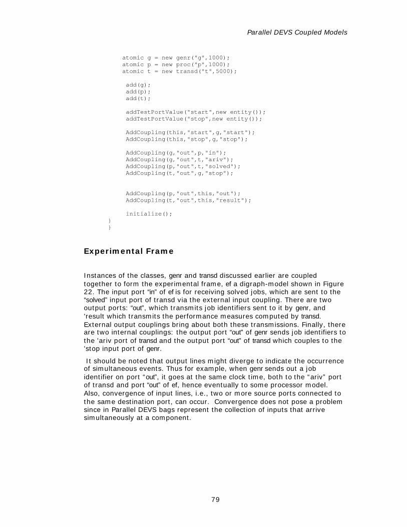
Parallel DEVS Coupled Models
79
atomic g = new genr("g",1000); atomic p = new proc("p",1000); atomic t = new transd("t",5000); add(g); add(p); add(t); addTestPortValue("start",new entity()); addTestPortValue("stop",new entity()); AddCoupling(this,"start",g,"start"); AddCoupling(this,"stop",g,"stop"); AddCoupling(g,"out",p,"in"); AddCoupling(g,"out",t,"ariv"); AddCoupling(p,"out",t,"solved"); AddCoupling(t,"out",g,"stop"); AddCoupling(p,"out",this,"out"); AddCoupling(t,"out",this,"result"); initialize(); } }
Experimental Frame
Instances of the classes, genr and transd discussed earlier are coupled together to form the experimental frame, ef a digraph-model shown in Figure 22. The input port “in” of ef is for receiving solved jobs, which are sent to the “solved” input port of transd via the external input coupling. There are two output ports: “out”, which transmits job identifiers sent to it by genr, and 'result which transmits the performance measures computed by transd. External output couplings bring about both these transmissions. Finally, there are two internal couplings: the output port “out” of genr sends job identifiers to the 'ariv port of transd and the output port “out” of transd which couples to the 'stop input port of genr.
It should be noted that output lines might diverge to indicate the occurrence of simultaneous events. Thus for example, when genr sends out a job identifier on port “out”, it goes at the same clock time, both to the “ariv” port of transd and port “out” of ef, hence eventually to some processor model. Also, convergence of input lines, i.e., two or more source ports connected to the same destination port, can occur. Convergence does not pose a problem since in Parallel DEVS bags represent the collection of inputs that arrive simultaneously at a component.
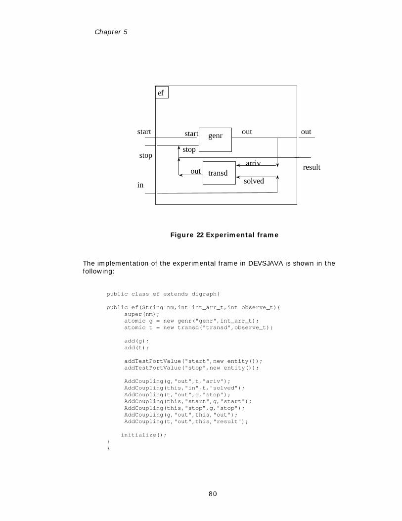
Chapter 5
80
start start outout
solved
arriv
genr
transd
stopstop
in
resultout
ef
Figure 22 Experimental frame
The implementation of the experimental frame in DEVSJAVA is shown in the following:
public class ef extends digraph{ public ef(String nm,int int_arr_t,int observe_t){ super(nm); atomic g = new genr("genr",int_arr_t); atomic t = new transd("transd",observe_t); add(g); add(t); addTestPortValue("start",new entity()); addTestPortValue("stop",new entity()); AddCoupling(g,"out",t,"ariv"); AddCoupling(this,"in",t,"solved"); AddCoupling(t,"out",g,"stop"); AddCoupling(this,"start",g,"start"); AddCoupling(this,"stop”,g,"stop"); AddCoupling(g,"out",this,"out"); AddCoupling(t,"out",this,"result"); initialize(); } }
Parallel DEVS Coupled Models
81
Hierarchical Models
Hierarchical models are coupled models with components that may be atomic or coupled models. Recall Figure 23 in which experimental frame, ef encapsulates a generator and a transducer into a coupled model. Figure 23 shows that an experimental frame can then be coupled to a processor to provide it with a stream of inputs (from the generator) and observe the statistics of the processor’s operation (the transducer). The processor can be an atomic model, as is the processor with buffer, for example, or can itself be a coupled model, for example, the pipeline coupled model in Figure 17. The “closure under coupling” property of DEVS, mentioned in Chapter 1, guarantees that coupled models can indeed be treated as basic models in larger coupled models. The simulation protocol was implemented in DEVSJAVA in such a way that closure under coupling and therefore, hierarchical model construction, will be supported.
out
in
processor
ef
in
outstart/stop
ef-p
Figure 23 Hierarchical model construction
Implementing Hierarchical Models in DEVSJAVA
Implementing a hierarchical model in DEVSJAVA is a “no-brainer” – you simply treat a coupled model as you would an atomic model as a component in a coupled model you are building. For example, in the following code, we assume that the digraph class, ef has already been defined. In constructing the enclosing hierarchical model, efp we make an instance of ef and couple it up with the processor component in the same was an atomic model would be treated. Likewise, if we want to replace the simple atomic processor by a pipeline-coupled model we would replace the definition of the variable p in the code by the line currently commented out.
Chapter 5
82
public class efp extends digraph { public efp (){ super("efp"); atomic p = new proc("proc",25); // digraph p = new pipeSimple(“pipe”, 20); digraph expf = new ef("ExpFrame",10,100); add(expf); add(p); AddCoupling(this,"start",expf,"start"); AddCoupling(this,"stop",expf,"stop"); AddCoupling(expf,"out",p,"in"); AddCoupling(p,"out",expf,"in"); initialize(); } }
Summary
Exercises
Exercise 1:
Define the coupled model for a cyclic pipeline and draw a state trajectory similar to that in Figure 19.
Exercise 2:
Consider a system consisting of a Heat Source and a Heat Sink. The heat source produces “heat impulses” at some constant time interval. Assume the Heat Source can be represented as an atomic model. The Heat Sink is a homogenous tube capable of absorbing heat impulses at one of its two ends (see figure below). Assume the tube is to be modeled as a flat two-dimensional homogeneous surface. Now consider a system (called Heat Transport) composed of the Heat Source and the Heat Sink where the former is placed at one of the ends of the latter (see figure below). The tube’s entire surface temperature is initially set to zero.
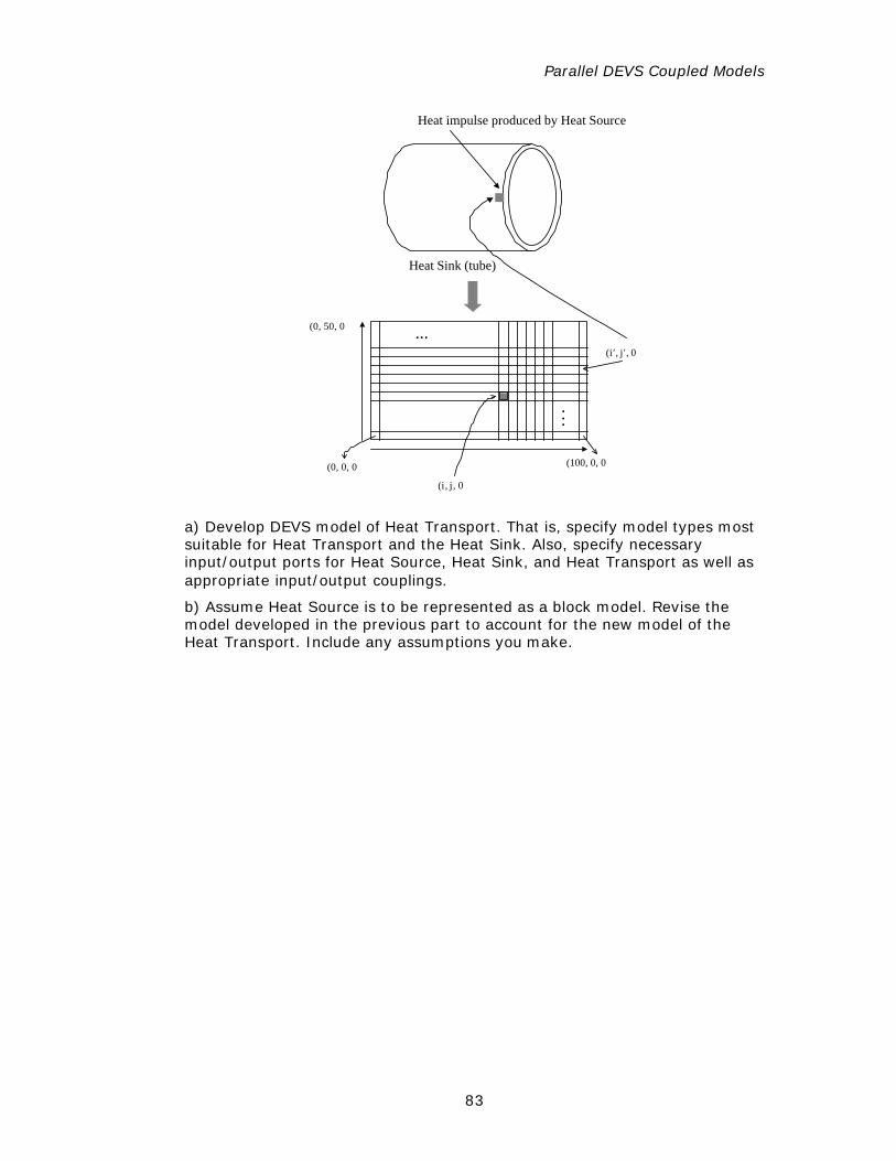
Parallel DEVS Coupled Models
83
(0, 0, 0) (100, 0, 0)
(i, j, 0)
(0, 50, 0)
(i′, j′, 0)
Heat impulse produced by Heat Source
Heat Sink (tube)
...
...
a) Develop DEVS model of Heat Transport. That is, specify model types most suitable for Heat Transport and the Heat Sink. Also, specify necessary input/output ports for Heat Source, Heat Sink, and Heat Transport as well as appropriate input/output couplings.
b) Assume Heat Source is to be represented as a block model. Revise the model developed in the previous part to account for the new model of the Heat Transport. Include any assumptions you make.
Chapter 6
EXERCISING MODELS: PARALLEL DEVS SIMULATION PROTOCOL
There are three approaches to parallel and distributed simulation of discrete event models: conservative, optimistic schemes, and the Parallel DEVS simulation protocol. In the conservative and optimistic schemes simulation is viewed as moved forward by the processing of time-stamped messages. In the third, DEVS-based approach, simulators are designed based directly on the DEVS formalism. The Parallel DEVS protocol can be viewed as an extreme form of risk-free optimism (not even local rollback occurs) and does not incur the overheads of conservative and optimistic schemes. Instead of trying to overlap processing of input events with different time-stamps, it seeks to exploit parallelism in the simultaneous occurrence of internal and external events (hence with the same, or closely spaced, time stamps) among many components.
Conservative and Optimistic Schemes
In the conservative and optimistic schemes simulation is viewed as moved forward by the processing of time-stamped messages. As depicted in Figure 24, such logical processors have input events queued in order of earliest time-stamp. Two laws govern processing:
q As a result of processing an input event, logical processors are assumed to produce output messages whose time-stamps are not earlier than the input time-stamp (processing can’t proceed backwards in time).
q Messages must be processed in order of time-stamps in the queues − schemes differ in how they treat this constraint.
In conservative schemes the time-stamped order constraint is never violated. Optimistic schemes allow temporary violation that must be repaired before the final simulation output is presented. The conservative approach is illustrated in Figure 24, where there are two logical processors LP1 and LP2 with queues of time stamped messages. We start in the upper left hand
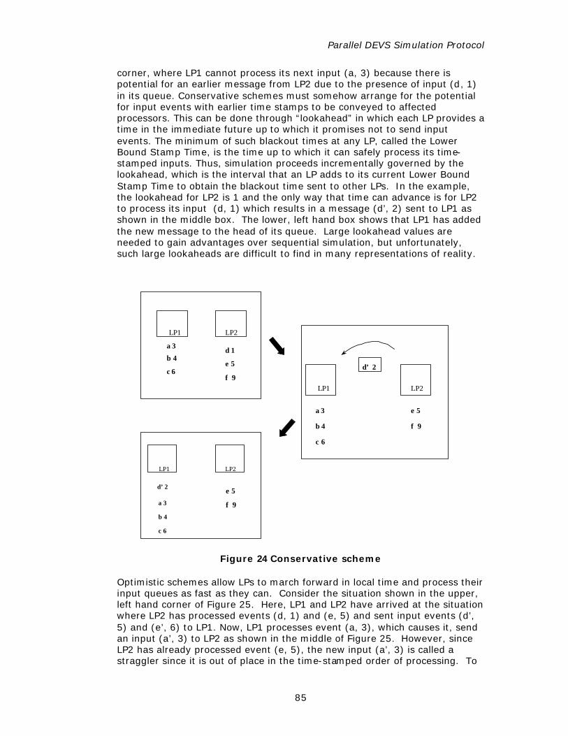
Parallel DEVS Simulation Protocol
85
corner, where LP1 cannot process its next input (a, 3) because there is potential for an earlier message from LP2 due to the presence of input (d, 1) in its queue. Conservative schemes must somehow arrange for the potential for input events with earlier time stamps to be conveyed to affected processors. This can be done through “lookahead” in which each LP provides a time in the immediate future up to which it promises not to send input events. The minimum of such blackout times at any LP, called the Lower Bound Stamp Time, is the time up to which it can safely process its time-stamped inputs. Thus, simulation proceeds incrementally governed by the lookahead, which is the interval that an LP adds to its current Lower Bound Stamp Time to obtain the blackout time sent to other LPs. In the example, the lookahead for LP2 is 1 and the only way that time can advance is for LP2 to process its input (d, 1) which results in a message (d’, 2) sent to LP1 as shown in the middle box. The lower, left hand box shows that LP1 has added the new message to the head of its queue. Large lookahead values are needed to gain advantages over sequential simulation, but unfortunately, such large lookaheads are difficult to find in many representations of reality.
a 3
b 4
c 6e 5
f 9
d 1
LP1 LP2
a 3
b 4
c 6
e 5
f 9
d’ 2
LP1 LP2
a 3
b 4
c 6
e 5
f 9
d’ 2
LP1 LP2
Figure 24 Conservative scheme
Optimistic schemes allow LPs to march forward in local time and process their input queues as fast as they can. Consider the situation shown in the upper, left hand corner of Figure 25. Here, LP1 and LP2 have arrived at the situation where LP2 has processed events (d, 1) and (e, 5) and sent input events (d’, 5) and (e’, 6) to LP1. Now, LP1 processes event (a, 3), which causes it, send an input (a’, 3) to LP2 as shown in the middle of Figure 25. However, since LP2 has already processed event (e, 5), the new input (a’, 3) is called a straggler since it is out of place in the time-stamped order of processing. To
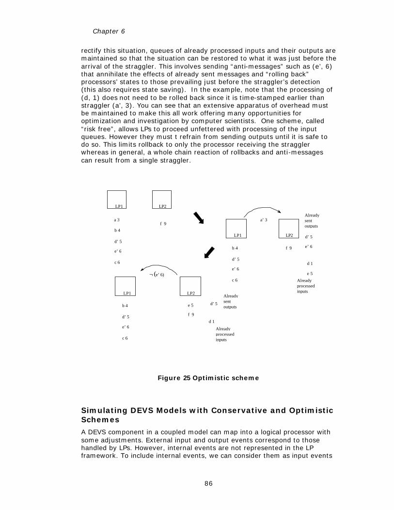
Chapter 6
86
rectify this situation, queues of already processed inputs and their outputs are maintained so that the situation can be restored to what it was just before the arrival of the straggler. This involves sending “anti-messages” such as (e’, 6) that annihilate the effects of already sent messages and “rolling back” processors’ states to those prevailing just before the straggler’s detection (this also requires state saving). In the example, note that the processing of (d, 1) does not need to be rolled back since it is time-stamped earlier than straggler (a’, 3). You can see that an extensive apparatus of overhead must be maintained to make this all work offering many opportunities for optimization and investigation by computer scientists. One scheme, called “risk free”, allows LPs to proceed unfettered with processing of the input queues. However they must t refrain from sending outputs until it is safe to do so. This limits rollback to only the processor receiving the straggler whereas in general, a whole chain reaction of rollbacks and anti-messages can result from a single straggler.
a’ 3
LP1 LP2
f 9 e’ 6
d’ 5
b 4
c 6
e’ 6
d’ 5
e 5
d 1
a 3f 9
LP1 LP2
b 4
c 6
e’ 6
d’ 5
LP1 LP2
¬(e’ 6)
b 4
c 6
e’ 6
d’ 5d 1
e 5
f 9
Alreadysentoutputs
Alreadyprocessedinputs
Alreadyprocessedinputs
Alreadysentoutputs
d’ 5
Figure 25 Optimistic scheme
Simulating DEVS Models with Conservative and Optimistic Schemes
A DEVS component in a coupled model can map into a logical processor with some adjustments. External input and output events correspond to those handled by LPs. However, internal events are not represented in the LP framework. To include internal events, we can consider them as input events
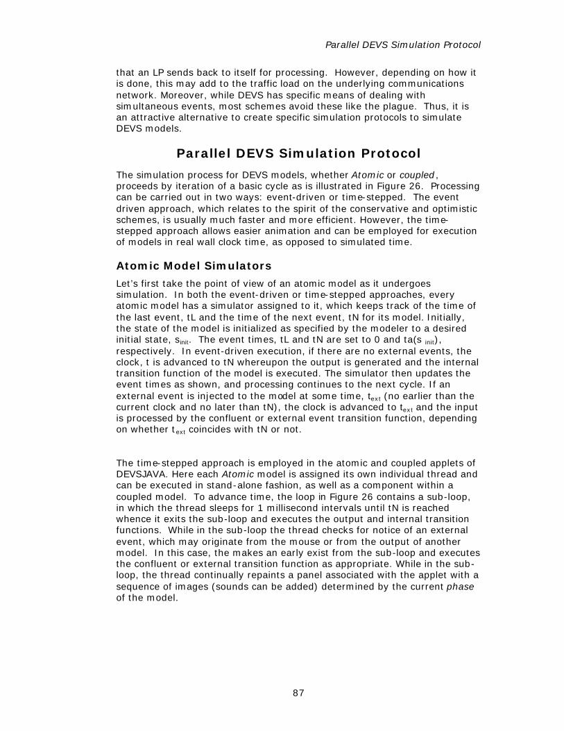
Parallel DEVS Simulation Protocol
87
that an LP sends back to itself for processing. However, depending on how it is done, this may add to the traffic load on the underlying communications network. Moreover, while DEVS has specific means of dealing with simultaneous events, most schemes avoid these like the plague. Thus, it is an attractive alternative to create specific simulation protocols to simulate DEVS models.
Parallel DEVS Simulation Protocol
The simulation process for DEVS models, whether Atomic or coupled, proceeds by iteration of a basic cycle as is illustrated in Figure 26. Processing can be carried out in two ways: event-driven or time-stepped. The event driven approach, which relates to the spirit of the conservative and optimistic schemes, is usually much faster and more efficient. However, the time-stepped approach allows easier animation and can be employed for execution of models in real wall clock time, as opposed to simulated time.
Atomic Model Simulators
Let’s first take the point of view of an atomic model as it undergoes simulation. In both the event-driven or time-stepped approaches, every atomic model has a simulator assigned to it, which keeps track of the time of the last event, tL and the time of the next event, tN for its model. Initially, the state of the model is initialized as specified by the modeler to a desired initial state, sinit. The event times, tL and tN are set to 0 and ta(s init), respectively. In event-driven execution, if there are no external events, the clock, t is advanced to tN whereupon the output is generated and the internal transition function of the model is executed. The simulator then updates the event times as shown, and processing continues to the next cycle. If an external event is injected to the model at some time, text (no earlier than the current clock and no later than tN), the clock is advanced to text and the input is processed by the confluent or external event transition function, depending on whether text coincides with tN or not.
The time-stepped approach is employed in the atomic and coupled applets of DEVSJAVA. Here each Atomic model is assigned its own individual thread and can be executed in stand-alone fashion, as well as a component within a coupled model. To advance time, the loop in Figure 26 contains a sub-loop, in which the thread sleeps for 1 millisecond intervals until tN is reached whence it exits the sub-loop and executes the output and internal transition functions. While in the sub-loop the thread checks for notice of an external event, which may originate from the mouse or from the output of another model. In this case, the makes an early exist from the sub-loop and executes the confluent or external transition function as appropriate. While in the sub-loop, the thread continually repaints a panel associated with the applet with a sequence of images (sounds can be added) determined by the current phase of the model.
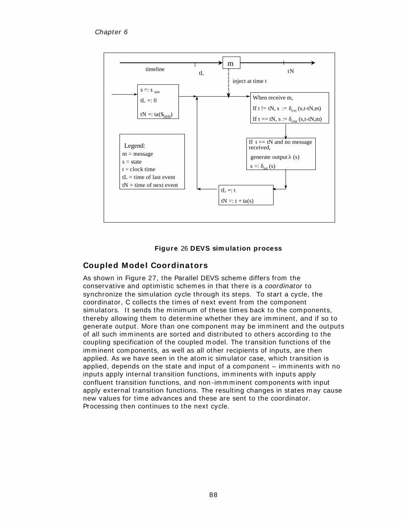
Chapter 6
88
tL =: t
tN =: t + ta(s)
When receive m,
If t != tN, s := δext (s,t-tN,m)
If t == tN, s := δcon (s,t-tN,m)
s =: s init
tL =: 0
tN =: ta(sinit)
mtimeline
inject at time t
tNtL
Legend:m = messages = statet = clock timetL = time of last eventtN = time of next event
If t == tN and no messagereceived,
generate output λ (s)
s =: δint (s)
Figure 26 DEVS simulation process
Coupled Model Coordinators
As shown in Figure 27, the Parallel DEVS scheme differs from the conservative and optimistic schemes in that there is a coordinator to synchronize the simulation cycle through its steps. To start a cycle, the coordinator, C collects the times of next event from the component simulators. It sends the minimum of these times back to the components, thereby allowing them to determine whether they are imminent, and if so to generate output. More than one component may be imminent and the outputs of all such imminents are sorted and distributed to others according to the coupling specification of the coupled model. The transition functions of the imminent components, as well as all other recipients of inputs, are then applied. As we have seen in the atomic simulator case, which transition is applied, depends on the state and input of a component – imminents with no inputs apply internal transition functions, imminents with inputs apply confluent transition functions, and non-immminent components with input apply external transition functions. The resulting changes in states may cause new values for time advances and these are sent to the coordinator. Processing then continues to the next cycle.
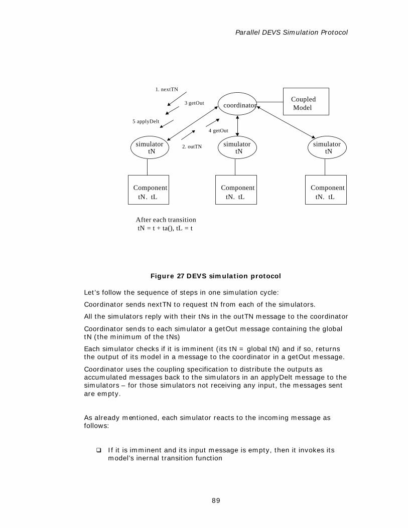
Parallel DEVS Simulation Protocol
89
coordinator
simulator
Component
tN
tN. tL
After each transition tN = t + ta(), tL = t
simulator
Component
tN
tN. tL
simulator
Component
tN
tN. tL
Coupled Model
1. nextTN
2. outTN
3 getOut
4 getOut
5 applyDelt
Figure 27 DEVS simulation protocol
Let’s follow the sequence of steps in one simulation cycle:
Coordinator sends nextTN to request tN from each of the simulators.
All the simulators reply with their tNs in the outTN message to the coordinator
Coordinator sends to each simulator a getOut message containing the global tN (the minimum of the tNs)
Each simulator checks if it is imminent (its tN = global tN) and if so, returns the output of its model in a message to the coordinator in a getOut message.
Coordinator uses the coupling specification to distribute the outputs as accumulated messages back to the simulators in an applyDelt message to the simulators – for those simulators not receiving any input, the messages sent are empty.
As already mentioned, each simulator reacts to the incoming message as follows:
q If it is imminent and its input message is empty, then it invokes its model’s inernal transition function
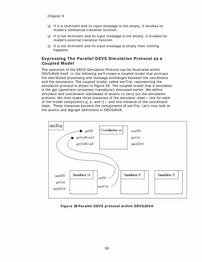
Chapter 6
90
q If it is imminent and its input message is not empty, it invokes its model’s confluence transition function
q If is not imminent and its input message is not empty, it invokes its model’s external transition function
q If is not imminent and its input message is empty then nothing happens.
Expressing The Parallel DEVS Simulation Protocol as a Coupled Model
The operation of the DEVS Simulation Protocol can be illustrated within DEVSJAVA itself. In the following we’ll create a coupled model that portrays the distributed processing and message exchanges between the coordinator and the simulators. The coupled model, called simTrip, representing the simulation protocol is shown in Figure 28. The coupled model that it simulates is the gpt (generator-processor-transducer) discussed earlier. We define simulator and coordinator subclasses of atomic to carry out the simulation protocol. We then make three instances of the simulator class – one for each of the model components g, p, and t) – and one instance of the coordinator class. These instances become the components of simTrip. Let’s now look at the atomic and digraph definitions in DEVSJAVA.
Figure 28 Parallel DEVS protocol within DEVSJAVA
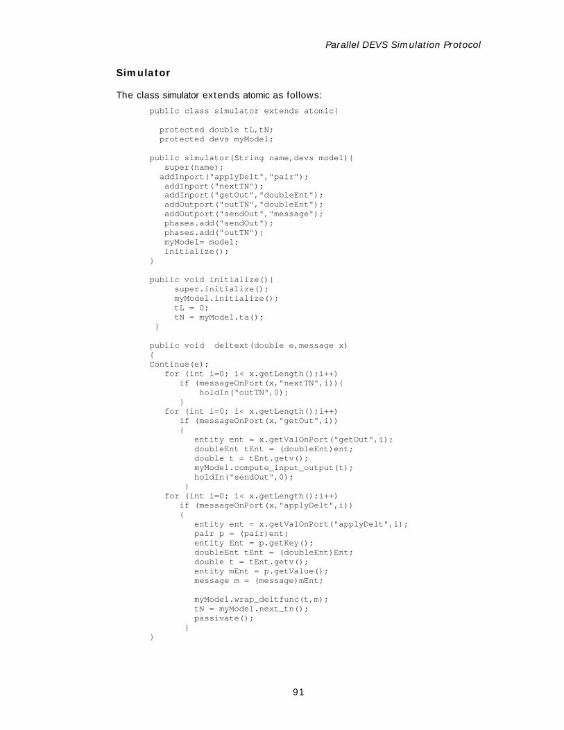
Parallel DEVS Simulation Protocol
91
Simulator
The class simulator extends atomic as follows:
public class simulator extends atomic{ protected double tL,tN; protected devs myModel; public simulator(String name,devs model){ super(name); addInport("applyDelt","pair"); addInport("nextTN"); addInport("getOut","doubleEnt"); addOutport("outTN","doubleEnt"); addOutport("sendOut","message"); phases.add("sendOut"); phases.add("outTN"); myModel= model; initialize(); } public void initialize(){ super.initialize(); myModel.initialize(); tL = 0; tN = myModel.ta(); } public void deltext(double e,message x) { Continue(e); for (int i=0; i< x.getLength();i++) if (messageOnPort(x,"nextTN",i)){ holdIn("outTN",0); } for (int i=0; i< x.getLength();i++) if (messageOnPort(x,"getOut",i)) { entity ent = x.getValOnPort("getOut",i); doubleEnt tEnt = (doubleEnt)ent; double t = tEnt.getv(); myModel.compute_input_output(t); holdIn("sendOut",0); } for (int i=0; i< x.getLength();i++) if (messageOnPort(x,"applyDelt",i)) { entity ent = x.getValOnPort("applyDelt",i); pair p = (pair)ent; entity Ent = p.getKey(); doubleEnt tEnt = (doubleEnt)Ent; double t = tEnt.getv(); entity mEnt = p.getValue(); message m = (message)mEnt; myModel.wrap_deltfunc(t,m); tN = myModel.next_tn(); passivate(); } }
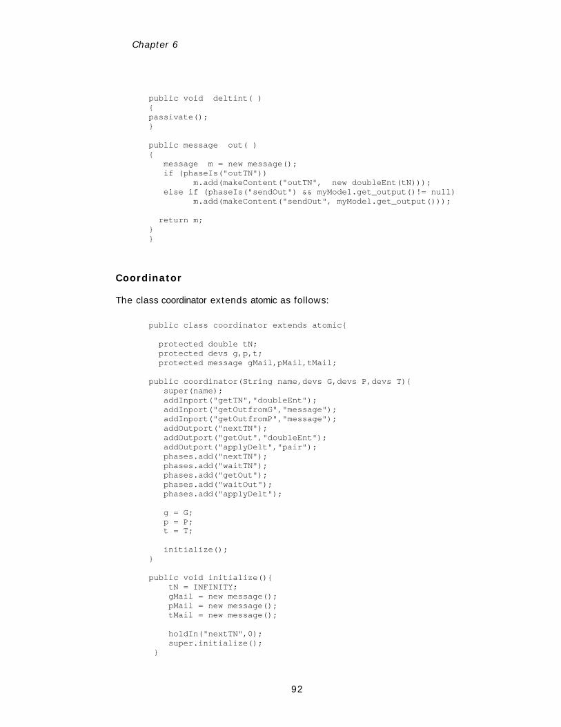
Chapter 6
92
public void deltint( ) { passivate(); } public message out( ) { message m = new message(); if (phaseIs("outTN")) m.add(makeContent("outTN", new doubleEnt(tN))); else if (phaseIs("sendOut") && myModel.get_output()!= null) m.add(makeContent("sendOut", myModel.get_output())); return m; } }
Coordinator
The class coordinator extends atomic as follows:
public class coordinator extends atomic{ protected double tN; protected devs g,p,t; protected message gMail,pMail,tMail; public coordinator(String name,devs G,devs P,devs T){ super(name); addInport("getTN","doubleEnt"); addInport("getOutfromG","message"); addInport("getOutfromP","message"); addOutport("nextTN"); addOutport("getOut","doubleEnt"); addOutport("applyDelt","pair"); phases.add("nextTN"); phases.add("waitTN"); phases.add("getOut"); phases.add("waitOut"); phases.add("applyDelt"); g = G; p = P; t = T; initialize(); } public void initialize(){ tN = INFINITY; gMail = new message(); pMail = new message(); tMail = new message(); holdIn("nextTN",0); super.initialize(); }
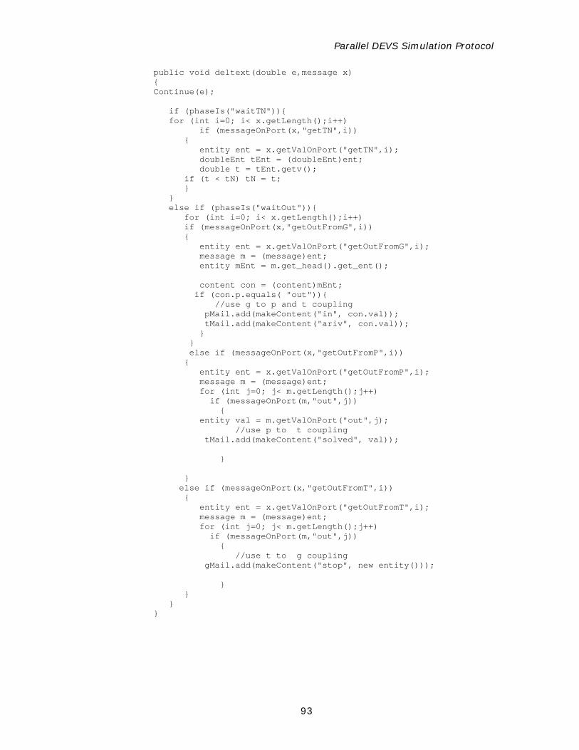
Parallel DEVS Simulation Protocol
93
public void deltext(double e,message x) { Continue(e); if (phaseIs("waitTN")){ for (int i=0; i< x.getLength();i++) if (messageOnPort(x,"getTN",i)) { entity ent = x.getValOnPort("getTN",i); doubleEnt tEnt = (doubleEnt)ent; double t = tEnt.getv(); if (t < tN) tN = t; } } else if (phaseIs("waitOut")){ for (int i=0; i< x.getLength();i++) if (messageOnPort(x,"getOutFromG",i)) { entity ent = x.getValOnPort("getOutFromG",i); message m = (message)ent; entity mEnt = m.get_head().get_ent(); content con = (content)mEnt; if (con.p.equals( "out")){ //use g to p and t coupling pMail.add(makeContent("in", con.val)); tMail.add(makeContent("ariv", con.val)); } } else if (messageOnPort(x,"getOutFromP",i)) { entity ent = x.getValOnPort("getOutFromP",i); message m = (message)ent; for (int j=0; j< m.getLength();j++) if (messageOnPort(m,"out",j)) { entity val = m.getValOnPort("out",j); //use p to t coupling tMail.add(makeContent("solved", val)); } } else if (messageOnPort(x,"getOutFromT",i)) { entity ent = x.getValOnPort("getOutFromT",i); message m = (message)ent; for (int j=0; j< m.getLength();j++) if (messageOnPort(m,"out",j)) { //use t to g coupling gMail.add(makeContent("stop", new entity())); } } } }
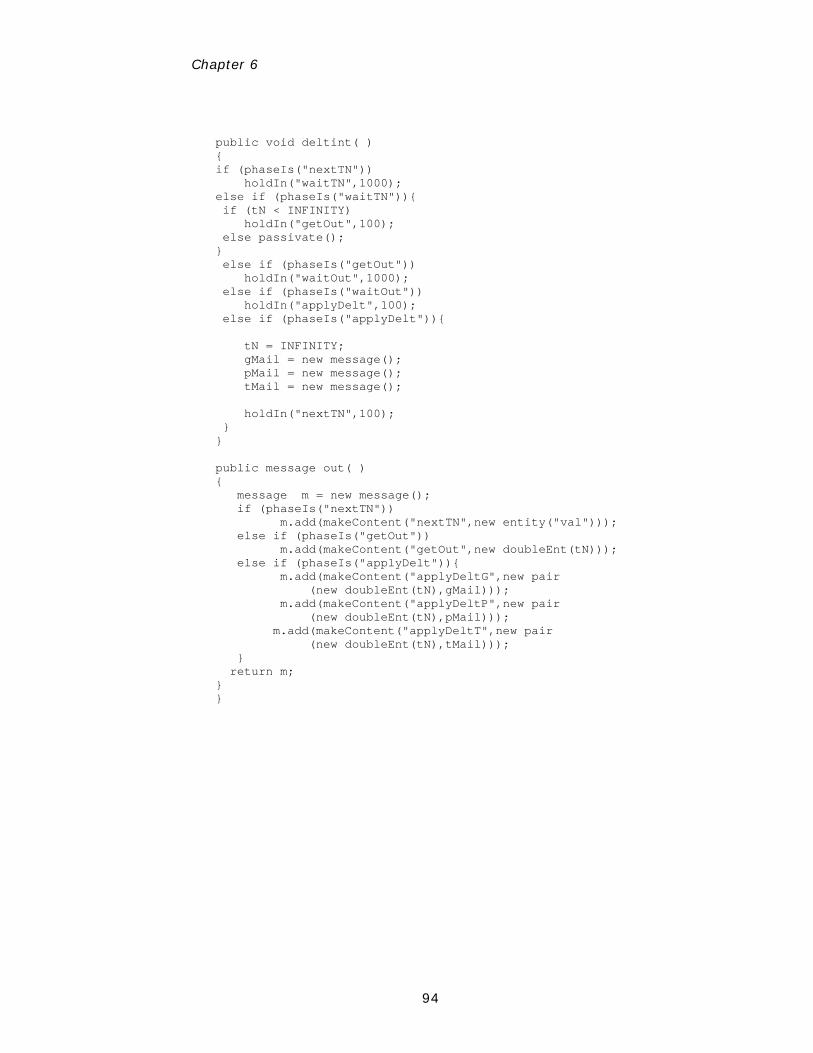
Chapter 6
94
public void deltint( ) { if (phaseIs("nextTN")) holdIn("waitTN",1000); else if (phaseIs("waitTN")){ if (tN < INFINITY) holdIn("getOut",100); else passivate(); } else if (phaseIs("getOut")) holdIn("waitOut",1000); else if (phaseIs("waitOut")) holdIn("applyDelt",100); else if (phaseIs("applyDelt")){ tN = INFINITY; gMail = new message(); pMail = new message(); tMail = new message(); holdIn("nextTN",100); } } public message out( ) { message m = new message(); if (phaseIs("nextTN")) m.add(makeContent("nextTN",new entity("val"))); else if (phaseIs("getOut")) m.add(makeContent("getOut",new doubleEnt(tN))); else if (phaseIs("applyDelt")){ m.add(makeContent("applyDeltG",new pair (new doubleEnt(tN),gMail))); m.add(makeContent("applyDeltP",new pair (new doubleEnt(tN),pMail))); m.add(makeContent("applyDeltT",new pair (new doubleEnt(tN),tMail))); } return m; } }
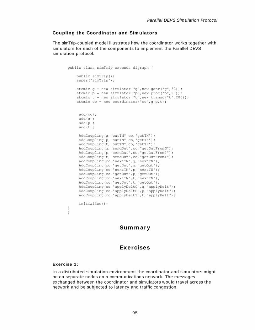
Parallel DEVS Simulation Protocol
95
Coupling the Coordinator and Simulators
The simTrip-coupled model illustrates how the coordinator works together with simulators for each of the components to implement the Parallel DEVS simulation protocol.
public class simTrip extends digraph { public simTrip(){ super("simTrip"); atomic g = new simulator("g",new genr("g",30)); atomic p = new simulator("p",new proc("p",20)); atomic t = new simulator("t",new transd("t",200)); atomic co = new coordinator("co",g,p,t); add(co); add(g); add(p); add(t); AddCoupling(g,"outTN",co,"getTN"); AddCoupling(p,"outTN",co,"getTN"); AddCoupling(t,"outTN",co,"getTN"); AddCoupling(g,"sendOut",co,"getOutFromG"); AddCoupling(p,"sendOut",co,"getOutFromP"); AddCoupling(t,"sendOut",co,"getOutFromT"); AddCoupling(co,"nextTN",g,"nextTN"); AddCoupling(co,"getOut",g,"getOut"); AddCoupling(co,"nextTN",p,"nextTN"); AddCoupling(co,"getOut",p,"getOut"); AddCoupling(co,"nextTN",t,"nextTN"); AddCoupling(co,"getOut",t,"getOut"); AddCoupling(co,"applyDeltG",g,"applyDelt"); AddCoupling(co,"applyDeltP",p,"applyDelt"); AddCoupling(co,"applyDeltT",t,"applyDelt"); initialize(); } }
Summary
Exercises
Exercise 1:
In a distributed simulation environment the coordinator and simulators might be on separate nodes on a communications network. The messages exchanged between the coordinator and simulators would travel across the network and be subjected to latency and traffic congestion.
Chapter 6
96
a) Add a message transducer as a component to the example as shown in Figure 28. The message transducer merely counts the number of messages that would flow across the network in a real distributed simulation.
Several modification of the implementation can be studied to reduce the message traffic while retaining the correctness of the simulation protocol.
b) Simulators need not reply with their next tNs if there is no change from the previous ones. This requires the coordinator to retain the previous tNs of the simulators. Modify the simulator and coordinator classes to implement this concept.
c) Instead of waiting for the coordinator’s getTN message, simulators provide their next tNs after completing their response to the coordinator’s applyDelt message. Further modify the simulator and coordinator classes of b) to implement this idea.
d) Run the digraph models of a), b) and c) with the same parameters given in the original DEVSJAVA code and record the number of messages exchanged as measured by the message transducer at the end.
e) Verify that the number of messages has been reduced as suggested and give a formula for the number of messages exchanged in one simulation cycle as a function of the number of simulators, n, (in the general case where there are n components) for protocols a), b) and c).
f) Suggest and implement some additional ways of reducing message traffic while retaining correctness.
Chapter 7
MULTIPROCESSOR ARCHITECTURES
Prototypical Processing Architectures
At this point, you have learned how to express atomic and coupled models in DEVSJAVA and you should have a working knowledge of how the underlying DEVS Parallel simulation protocol works. More particularly, in Chapter 6 we constructed a hierarchical model coupling up a simple processor model with an experimental frame. This chapter will show how design some prototypical multiprocessor architectures to replace the simple processor in such a pair and compare their performance under the same conditions. The model domain to be discussed is that of simple workflow architectures such as in distributed computing, office systems, assembly lines and communication systems. We are interested in comparing the performance of single processor systems with multiprocessors including the multiserver, the pipeline, and the divide and conquer configurations. Performance evaluation will be based on two fundamental measures, turnaround time, the average time taken by the system to solve a problem and throughput, the rate at which completed jobs emerge from the system.
The multiprocessor configurations to be modeled each have a coordinator that sends jobs (jobs) to some subordinate processors and receives solutions from them. In the multiserver architecture, the coordinator routes incoming jobs to whichever processor is free at the time. In the pipeline architecture, jobs pass through the processors in a, sequence, each processor performing a part of the solution. Our model can be called a “soft” pipeline. In contrast to typical hardware pipelines, the problems are routed by the coordinator from one processor to the next under a programmable schedule. In the divide and conquer architecture, jobs are decomposed into subtasks that are worked on concurrently and independently by the processors before being be put together to form the final solution.
The multiprocessor architectures are prototypical in the sense that forms of coordination they represent can be found in many diverse applications. Their implementation in DEVSJAVA illustrates how sophisticated coordination schemes can be modeled and simulated.
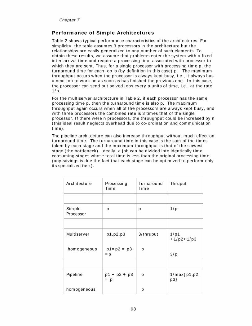
Chapter 7
98
Performance of Simple Architectures
Table 2 shows typical performance characteristics of the architectures. For simplicity, the table assumes 3 processors in the architecture but the relationships are easily generalized to any number of such elements. To obtain these results, we assume that problems enter the system with a fixed inter-arrival time and require a processing time associated with processor to which they are sent. Thus, for a single processor with processing time p, the turnaround time for each job is (by definition in this case) p. The maximum throughput occurs when the processor is always kept busy, i.e., it always has a next job to work on as soon as has finished the previous one. In this case, the processor can send out solved jobs every p units of time, i.e., at the rate 1/p.
For the multiserver architecture in Table 2, if each processor has the same processing time p, then the turnaround time is also p. The maximum throughput again occurs when all of the processors are always kept busy, and with three processors the combined rate is 3 times that of the single processor. If there were n processors, the throughput could be increased by n (this ideal result neglects overhead due to co-ordination and communication time).
The pipeline architecture can also increase throughput without much effect on turnaround time. The turnaround time in this case is the sum of the times taken by each stage and the maximum throughput is that of the slowest stage (the bottleneck). Ideally, a job can be divided into identically time consuming stages whose total time is less than the original processing time (any savings is due the fact that each stage can be optimized to perform only its specialized task).
Architecture Processing Time
Turnaround Time
Thruput
Simple Processor
p p 1/p
Multiserver
homogeneous
p1,p2,p3
p1=p2 = p3 =p
3/thruput
p
1/p1 +1/p2+1/p3
3/p
Pipeline
homogeneous
p1 + p2 + p3 = p
p
p
1/max{p1,p2,p3}
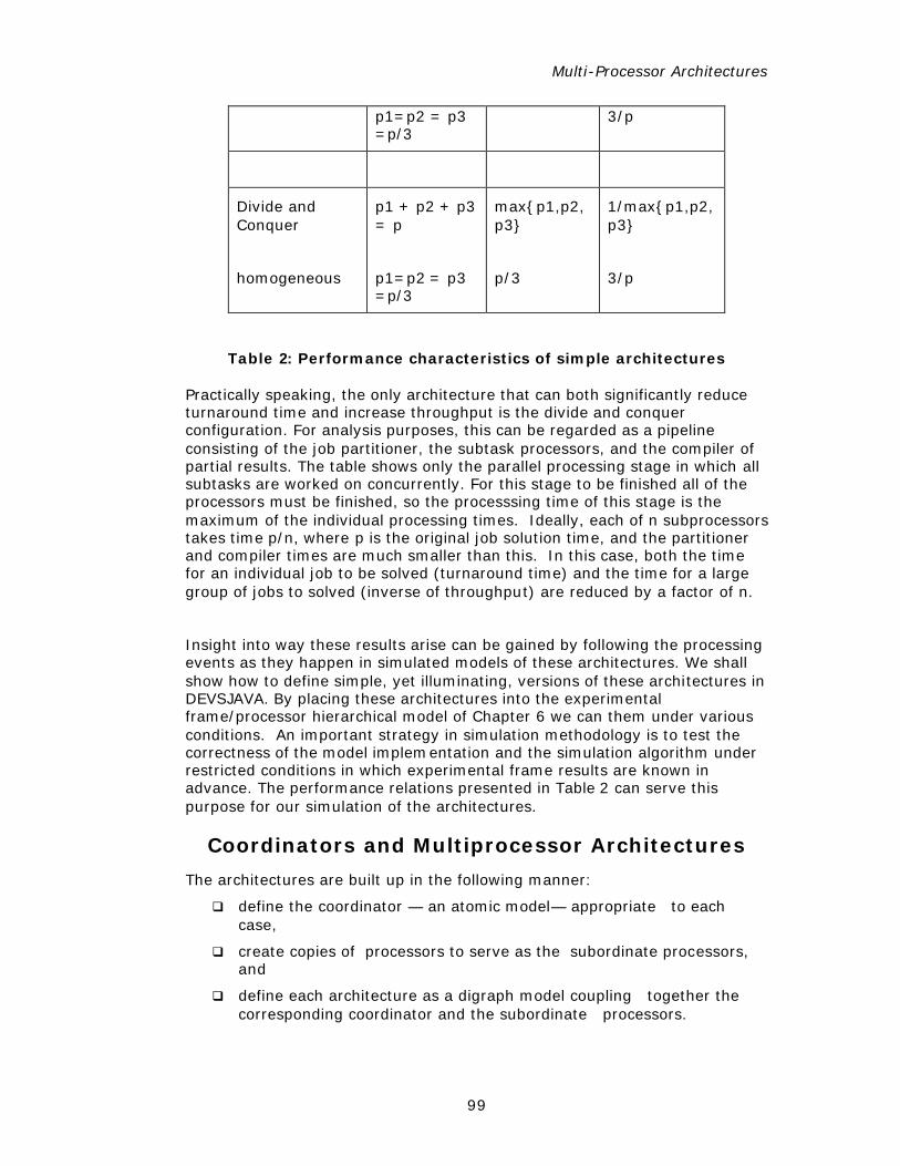
Multi-Processor Architectures
99
p1=p2 = p3 =p/3
3/p
Divide and Conquer
homogeneous
p1 + p2 + p3 = p
p1=p2 = p3 =p/3
max{p1,p2,p3}
p/3
1/max{p1,p2,p3}
3/p
Table 2: Performance characteristics of simple architectures
Practically speaking, the only architecture that can both significantly reduce turnaround time and increase throughput is the divide and conquer configuration. For analysis purposes, this can be regarded as a pipeline consisting of the job partitioner, the subtask processors, and the compiler of partial results. The table shows only the parallel processing stage in which all subtasks are worked on concurrently. For this stage to be finished all of the processors must be finished, so the processsing time of this stage is the maximum of the individual processing times. Ideally, each of n subprocessors takes time p/n, where p is the original job solution time, and the partitioner and compiler times are much smaller than this. In this case, both the time for an individual job to be solved (turnaround time) and the time for a large group of jobs to solved (inverse of throughput) are reduced by a factor of n.
Insight into way these results arise can be gained by following the processing events as they happen in simulated models of these architectures. We shall show how to define simple, yet illuminating, versions of these architectures in DEVSJAVA. By placing these architectures into the experimental frame/processor hierarchical model of Chapter 6 we can them under various conditions. An important strategy in simulation methodology is to test the correctness of the model implementation and the simulation algorithm under restricted conditions in which experimental frame results are known in advance. The performance relations presented in Table 2 can serve this purpose for our simulation of the architectures.
Coordinators and Multiprocessor Architectures
The architectures are built up in the following manner:
q define the coordinator — an atomic model— appropriate to each case,
q create copies of processors to serve as the subordinate processors, and
q define each architecture as a digraph model coupling together the corresponding coordinator and the subordinate processors.
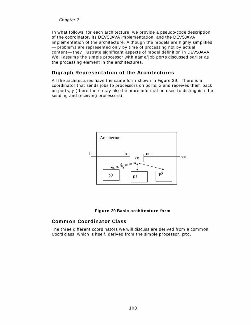
Chapter 7
100
In what follows, for each architecture, we provide a pseudo-code description of the coordinator, its DEVSJAVA implementation, and the DEVSJAVA implementation of the architecture. Although the models are highly simplified — problems are represented only by time of processing not by actual content— they illustrate significant aspects of model definition in DEVSJAVA. We’ll assume the simple processor with name/job ports discussed earlier as the processing element in the architectures.
Digraph Representation of the Architectures
All the architectures have the same form shown in Figure 29. There is a coordinator that sends jobs to processors on ports, x and receives them back on ports, y (there there may also be more information used to distinguish the sending and receiving processors).
in inout
out
xy
co
p0 p1 p2
Architecture
Figure 29 Basic architecture form
Common Coordinator Class
The three different coordinators we will discuss are derived from a common Coord class, which is itself, derived from the simple processor, proc.
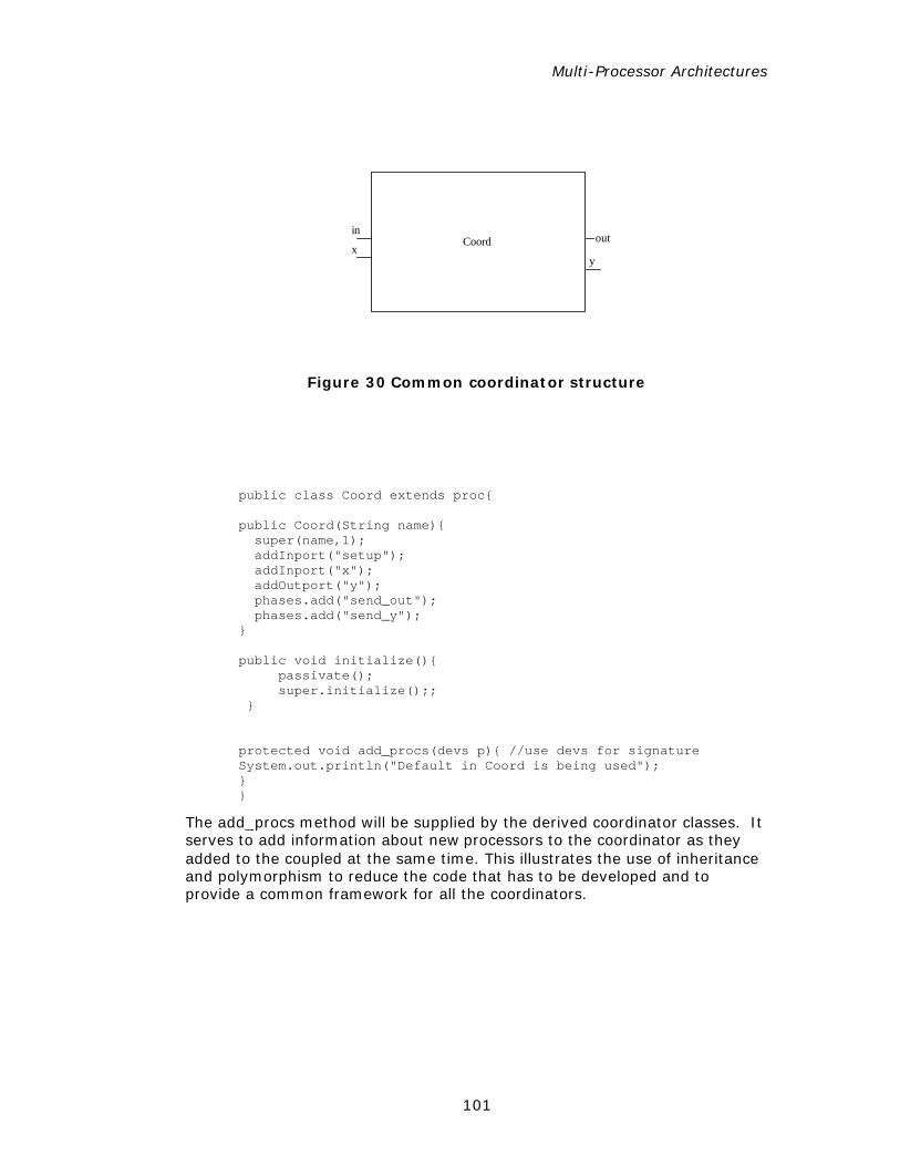
Multi-Processor Architectures
101
inoutCoord
xy
Figure 30 Common coordinator structure
public class Coord extends proc{ public Coord(String name){ super(name,1); addInport("setup"); addInport("x"); addOutport("y"); phases.add("send_out"); phases.add("send_y"); } public void initialize(){ passivate(); super.initialize();; } protected void add_procs(devs p){ //use devs for signature System.out.println("Default in Coord is being used"); } }
The add_procs method will be supplied by the derived coordinator classes. It serves to add information about new processors to the coordinator as they added to the coupled at the same time. This illustrates the use of inheritance and polymorphism to reduce the code that has to be developed and to provide a common framework for all the coordinators.
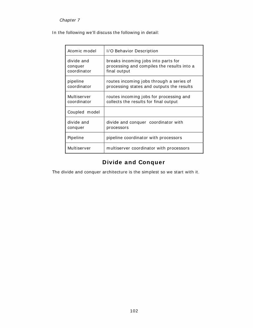
Chapter 7
102
In the following we’ll discuss the following in detail:
Atomic model I/O Behavior Description
divide and conquer coordinator
breaks incoming jobs into parts for processing and compiles the results into a final output
pipeline coordinator
routes incoming jobs through a series of processing states and outputs the results
Multiserver coordinator
routes incoming jobs for processing and collects the results for final output
Coupled model
divide and conquer
divide and conquer coordinator with processors
Pipeline pipeline coordinator with processors
Multiserver multiserver coordinator with processors
Divide and Conquer
The divide and conquer architecture is the simplest so we start with it.
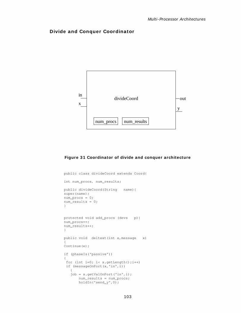
Multi-Processor Architectures
103
Divide and Conquer Coordinator
inoutdivideCoord
xy
num_procs num_results
Figure 31 Coordinator of divide and conquer architecture
public class divideCoord extends Coord{ int num_procs, num_results; public divideCoord(String name){ super(name); num_procs = 0; num_results = 0; } protected void add_procs (devs p){ num_procs++; num_results++; } public void deltext(int e,message x) { Continue(e); if (phaseIs("passive")) { for (int i=0; i< x.getLength();i++) if (messageOnPort(x,"in",i)) { job = x.getValOnPort("in",i); num_results = num_procs; holdIn("send_y",0);
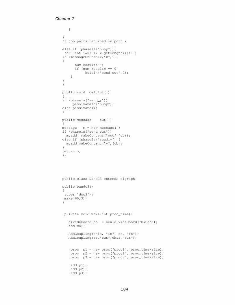
Chapter 7
104
} } // job pairs returned on port x else if (phaseIs("busy")){ for (int i=0; i< x.getLength();i++) if (messageOnPort(x,"x",i)) { num_results--; if (num_results == 0) holdIn("send_out",0); } } } public void deltint( ) { if (phaseIs("send_y")) passivateIn("busy"); else passivate(); } public message out( ) { message m = new message(); if (phaseIs("send_out")) m.add( makeContent("out",job)); else if (phaseIs("send_y")){ m.add(makeContent("y",job); } return m; })
public class DandC3 extends digraph{ public DandC3() { super("d&c3"); make(60,3); } private void make(int proc_time){ divideCoord co = new divideCoord("D&Cco"); add(co); AddCoupling(this, "in", co, "in"); AddCoupling(co,"out",this,"out"); proc p1 = new proc("proc1", proc_time/size); proc p2 = new proc("proc2", proc_time/size); proc p3 = new proc("proc3", proc_time/size); add(p1); add(p2); add(p3);

Multi-Processor Architectures
105
co.add_procs(p1); co.add_procs(p2); co.add_procs(p3); AddCoupling(co, "y", p1,"in"); AddCoupling(p1,"out",co,"x"); AddCoupling(co, "y", p2,"in"); AddCoupling(p2,"out",co,"x"); AddCoupling(co, "y", p3,"in"); AddCoupling(p3,"out",co,"x"); initialize(); } }
Divide and Conquer Architecture
Behavior of Divide and Conquer Architecture
Let us trace a typical state trajectory to illustrate the operation of the divide and conquer architecture. We start in an initial state in which the coordinator and all subordinate processors are idle. In the experimental frame discussed earlier, problems will arrive on port “in” of divideCoord from the generator. Solved problems will leave on port “out” for the transducer. A typical state trajectory for the divide and conquer architecture is shown in Figure 32. You will see that the three processors act in effect, as one stage in the sequence from input to output. This is so since to accept a new job divideCoord requires that all processors have finished the subtasks of the current job. Since they are processed concurrently, the time to solve all subtasks is the time taken to finish the longest one.
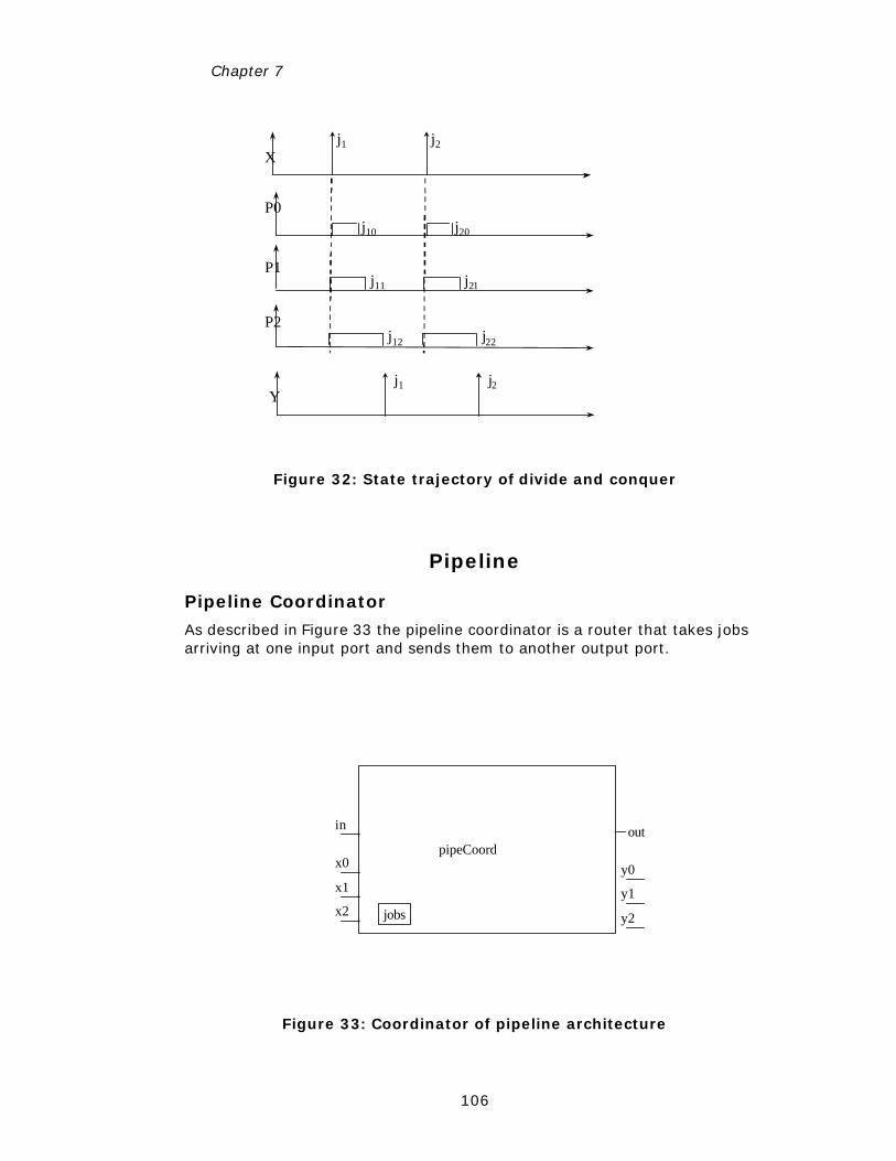
Chapter 7
106
P0
j1
j10
P1
P2
j11
j12
X
j1Y
j2
j20
j21
j22
j2
Figure 32: State trajectory of divide and conquer
Pipeline
Pipeline Coordinator
As described in Figure 33 the pipeline coordinator is a router that takes jobs arriving at one input port and sends them to another output port.
in outpipeCoord
x0
jobs
x1
x2
y0
y1
y2
Figure 33: Coordinator of pipeline architecture
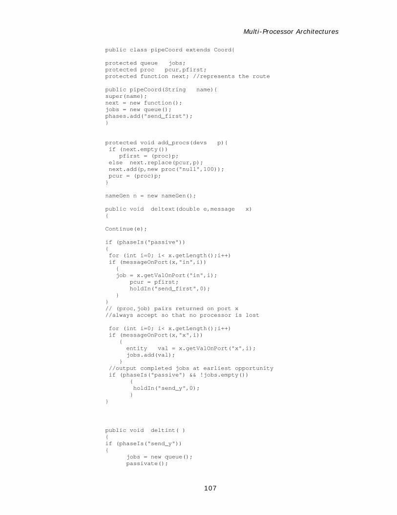
Multi-Processor Architectures
107
public class pipeCoord extends Coord{ protected queue jobs; protected proc pcur,pfirst; protected function next; //represents the route public pipeCoord(String name){ super(name); next = new function(); jobs = new queue(); phases.add("send_first"); } protected void add_procs(devs p){ if (next.empty()) pfirst = (proc)p; else next.replace(pcur,p); next.add(p,new proc("null",100)); pcur = (proc)p; } nameGen n = new nameGen(); public void deltext(double e,message x) { Continue(e); if (phaseIs("passive")) { for (int i=0; i< x.getLength();i++) if (messageOnPort(x,"in",i)) { job = x.getValOnPort("in",i); pcur = pfirst; holdIn("send_first",0); } } // (proc,job) pairs returned on port x //always accept so that no processor is lost for (int i=0; i< x.getLength();i++) if (messageOnPort(x,"x",i)) { entity val = x.getValOnPort("x",i); jobs.add(val); } //output completed jobs at earliest opportunity if (phaseIs("passive") && !jobs.empty()) { holdIn("send_y",0); } }
public void deltint( ) { if (phaseIs("send_y")) { jobs = new queue(); passivate();
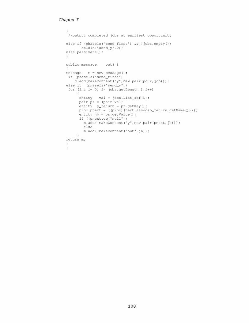
Chapter 7
108
} //output completed jobs at earliest opportunity else if (phaseIs("send_first") && !jobs.empty()) holdIn("send_y",0); else passivate(); } public message out( ) { message m = new message(); if (phaseIs("send_first")) m.add(makeContent("y",new pair(pcur,job))); else if (phaseIs("send_y")) for (int i= 0; i< jobs.getLength();i++) { entity val = jobs.list_ref(i); pair pr = (pair)val; entity p_return = pr.getKey(); proc pnext = ((proc)(next.assoc(p_return.getName()))); entity jb = pr.getValue(); if (!pnext.eq("null")) m.add( makeContent("y",new pair(pnext,jb))); else m.add( makeContent("out",jb)); } return m; } }
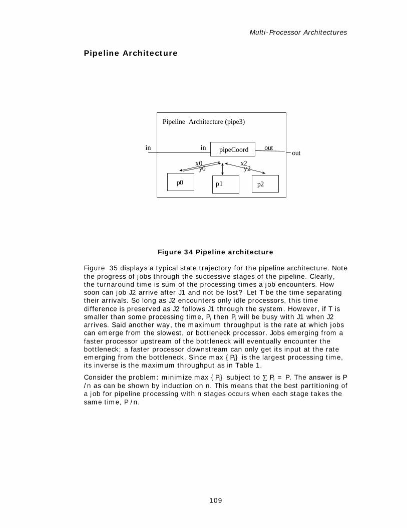
Multi-Processor Architectures
109
Pipeline Architecture
in inout
out
x0y0
pipeCoord
p0 p1 p2
Pipeline Architecture (pipe3)
x2y2
Figure 34 Pipeline architecture
Figure 35 displays a typical state trajectory for the pipeline architecture. Note the progress of jobs through the successive stages of the pipeline. Clearly, the turnaround time is sum of the processing times a job encounters. How soon can job J2 arrive after J1 and not be lost? Let T be the time separating their arrivals. So long as J2 encounters only idle processors, this time difference is preserved as J2 follows J1 through the system. However, if T is smaller than some processing time, Pi then Pi will be busy with J1 when J2 arrives. Said another way, the maximum throughput is the rate at which jobs can emerge from the slowest, or bottleneck processor. Jobs emerging from a faster processor upstream of the bottleneck will eventually encounter the bottleneck; a faster processor downstream can only get its input at the rate emerging from the bottleneck. Since max {Pi} is the largest processing time, its inverse is the maximum throughput as in Table 1.
Consider the problem: minimize max {Pi} subject to ∑ PI = P. The answer is P /n as can be shown by induction on n. This means that the best partitioning of a job for pipeline processing with n stages occurs when each stage takes the same time, P /n.
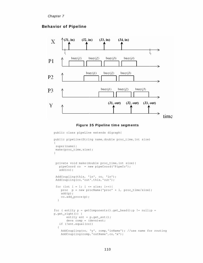
Chapter 7
110
Behavior of Pipeline
Figure 35 Pipeline time segments
public class pipeLine extends digraph{ public pipeLine(String name,double proc_time,int size) { super(name); make(proc_time,size); } private void make(double proc_time,int size){ pipeCoord co = new pipeCoord("PipeCo"); add(co); AddCoupling(this, "in", co, "in"); AddCoupling(co,"out",this,"out"); for (int i = 1; i <= size; i++){ proc p = new procName("proc" + i, proc_time/size); add(p); co.add_procs(p); } for ( entity p = getComponents().get_head();p != null;p = p.get_right()) { entity ent = p.get_ent(); devs comp = (devs)ent; if (!ent.equal(co)) { AddCoupling(co, "y", comp,"inName"); //use name for routing AddCoupling(comp,"outName",co,"x");
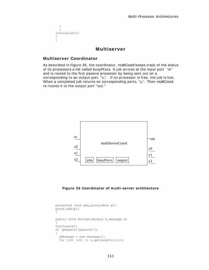
Multi-Processor Architectures
111
} } initialize(); } }
Multiserver
Multiserver Coordinator
As described in Figure 36, the coordinator, multiCoord keeps track of the status of its processors a list called busyProcs. A job arrives at the input port “in” and is routed to the first passive processor by being sent out on a corresponding to an output port, “xi“. If no processor is free, the job is lost. When a completed job returns on corresponding ports, “yi“. Then multiCoord re-routes it to the output port “out.”
in outmultiServerCoord
x0
jobs
x1
x2
y0
y1
y2busyProcs outport
Figure 36 Coordinator of multi-server architecture
protected void add_procs(devs p){ procs.add(p); } public void deltext(double e,message x) { Continue(e); if (phaseIs("passive")) { yMessage = new message(); for (int i=0; i< x.getLength();i++)
Chapter 7
112
if (messageOnPort(x,"in",i)) { job = x.getValOnPort("in",i); if ( !procs.empty()) { entity pcur = procs.front(); procs.remove(); yMessage.add(makeContent("y",new pair(pcur,job))); holdIn("send_y",0); } } } // (proc,job) pairs returned on port x //always accept so that no processor is lost for (int i=0; i< x.getLength();i++) if (messageOnPort(x,"x",i)) { entity val = x.getValOnPort("x",i); pair pr = (pair)val; procs.add(pr.getKey()); entity jb = pr.getValue(); jobs.add(jb); } //output completed jobs at earliest opportunity if (phaseIs("passive") && !jobs.empty()) holdIn("send_out",0); } public void deltint( ) { if (phaseIs("send_out")) { jobs = new queue(); passivate(); } //output completed jobs at earliest opportunity else if (phaseIs("send_y") && !jobs.empty()) holdIn("send_out",0); else passivate(); } public message out( ) { message m = new message(); if (phaseIs("send_out")) for (int i= 0; i< jobs.getLength();i++) { entity job = jobs.list_ref(i); m.add( makeContent("out",job)); } else if (phaseIs("send_y")) m = yMessage; return m; } }
Multi-Processor Architectures
113
Multiserver Architecture
The coupling of the multiserver architecture follows exactly the form of the pipeline architecture with replacement the corresponding coordinator of the processors. Specifying the digraph model is therefore a straightforward revision.
public class multiServer extends digraph{ public multiServer(String name,double proc_time,int size) { super(name); make(proc_time,size); } private void make(double proc_time,int size){ multiServerCoord co = new multiServerCoord("MultiSco"); add(co); for (int i = 1; i <= size; i++){ proc p = new procName("proc" + i, proc_time); add(p); co.add_procs(p); } for (entity p = getComponents().get_head();p != null;p = p.get_right()) { entity ent = p.get_ent(); devs comp = (devs)ent; if (!ent.equal(co)) { AddCoupling(co, "y", comp,"inName"); //use name for routing AddCoupling(comp,"outName",co,"x"); } } AddCoupling(this,"in",co,"in"); AddCoupling(co,"out",this,"out"); initialize(); } }
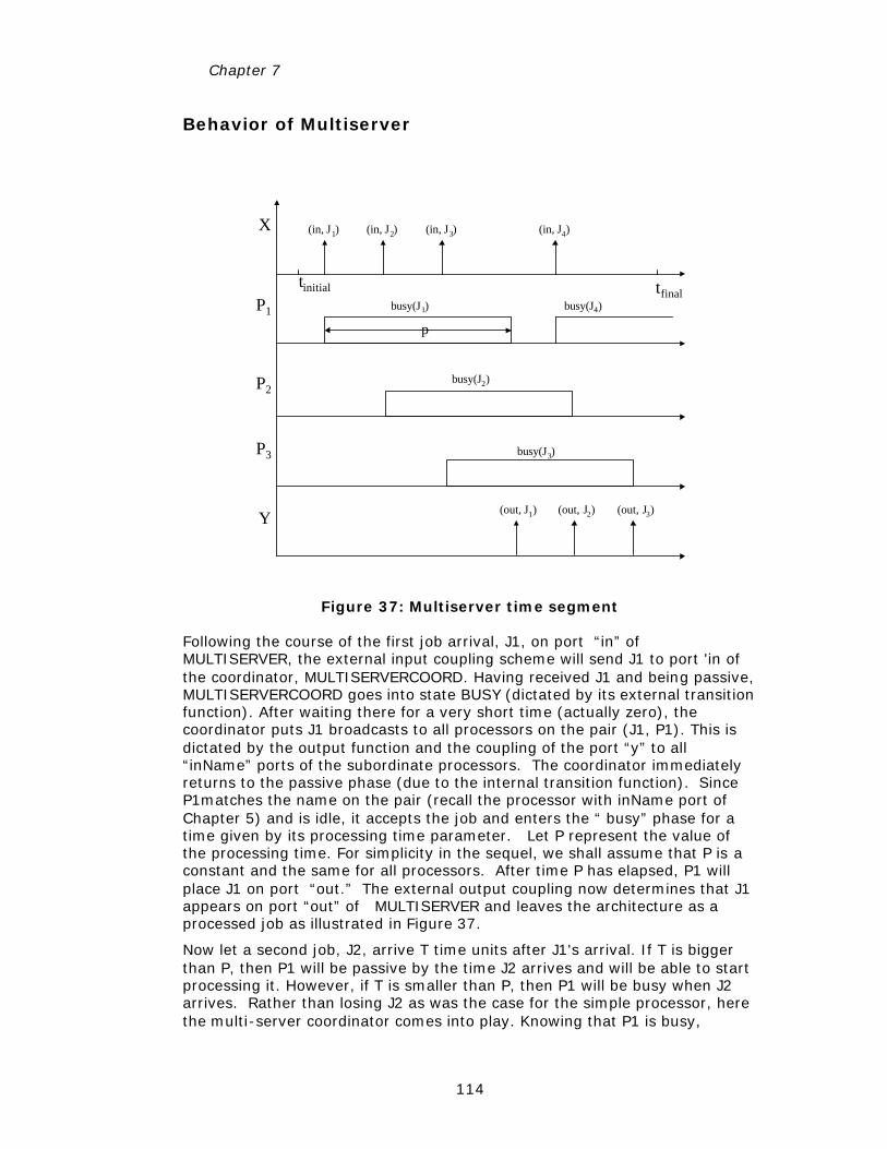
Chapter 7
114
Behavior of Multiserver
(in, J1)X
P1
P2
P3
Y
(in, J2) (in, J3) (in, J4)
p
busy(J1)
busy(J3)
busy(J2)
busy(J4)
(out, J1) (out, J3)(out, J2)
tinitial tfinal
Figure 37: Multiserver time segment
Following the course of the first job arrival, J1, on port “in” of MULTISERVER, the external input coupling scheme will send J1 to port 'in of the coordinator, MULTISERVERCOORD. Having received J1 and being passive, MULTISERVERCOORD goes into state BUSY (dictated by its external transition function). After waiting there for a very short time (actually zero), the coordinator puts J1 broadcasts to all processors on the pair (J1, P1). This is dictated by the output function and the coupling of the port “y” to all “inName” ports of the subordinate processors. The coordinator immediately returns to the passive phase (due to the internal transition function). Since P1matches the name on the pair (recall the processor with inName port of Chapter 5) and is idle, it accepts the job and enters the “ busy” phase for a time given by its processing time parameter. Let P represent the value of the processing time. For simplicity in the sequel, we shall assume that P is a constant and the same for all processors. After time P has elapsed, P1 will place J1 on port “out.” The external output coupling now determines that J1 appears on port “out” of MULTISERVER and leaves the architecture as a processed job as illustrated in Figure 37.
Now let a second job, J2, arrive T time units after J1's arrival. If T is bigger than P, then P1 will be passive by the time J2 arrives and will be able to start processing it. However, if T is smaller than P, then P1 will be busy when J2 arrives. Rather than losing J2 as was the case for the simple processor, here the multi-server coordinator comes into play. Knowing that P1 is busy,
Multi-Processor Architectures
115
MULTISERVERCOORD sends J2 to the next free processor, P2 using the name-directed broadcasting just discussed.
For simplicity, assume that there are 3 processors. Then a third job, J3, arriving while both P1 and P2 are busy, will be sent to P3. However, a fourth job that arrives while all processors are busy will be lost. As illustrated in Figure 37, if the job inter-arrival-time, T, is a constant, equal to P /3, then the fourth and subsequent jobs arrive just after a (exactly one) processor has finished its work. The figure makes clear that this is an arrival pattern in which processors are always kept busy. The emerging jobs are separated in time by P /3 so that the throughput is 3/P. Since the processors are always kept busy, there is no way to produce a higher rate of job completions. Thus we can justify the entry for the multi-server architecture with constant processing time in Table 2. Clearly, each job still takes time P units to be processed, so that the average turnaround time is P.
In the case of heterogeneous processing times, {Pi}, the fastest that each processor, Pi can emit jobs is at rate 1/min {Pi}. The maximum throughput is the sum of these rates. The average turnaround time associated with this departure rate can be obtained by considering the mix of jobs at any time. The number of jobs processed in a long period is proportional to 1/throughput. Of these, there are 1/Pi jobs in the ith processor and these take time Pi to complete, yielding the average contribution of the ith processor of Pi * 1/(Pi*throughput) which equals 1/throughput. For n processors, the average turnaround time is therefore n/throughput. This accounts for the corresponding entry in Table 2.
The same result can be derived from Little's relation (Sauer and Chandy 80): The average turnaround time = the average number of jobs in the system / the job departure rate
Note that Little's formula relates the three performance indexes, work in process (jobs in the system), throughput and turnaround time. It claims that usually the latter are inverses of each other, just as intuition would have us imagine. However, it holds only for certain kinds of systems in which jobs are distributed uniformly around the processors at all times.
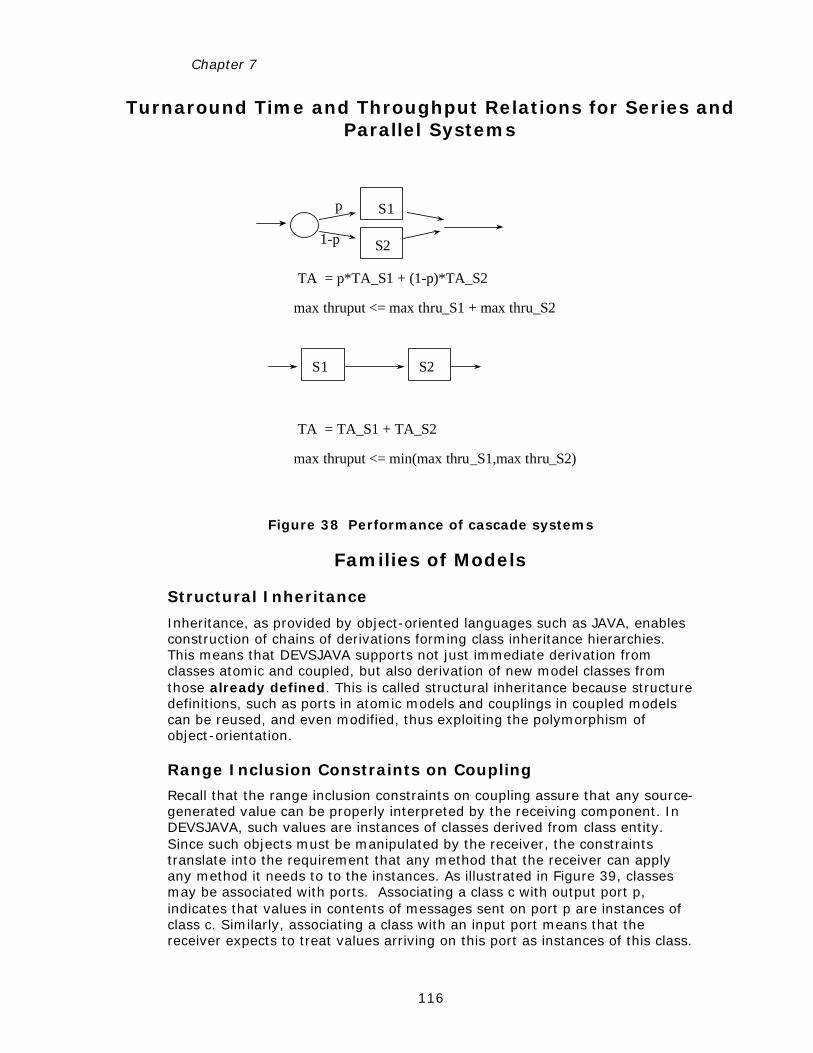
Chapter 7
116
Turnaround Time and Throughput Relations for Series and Parallel Systems
max thruput <= min(max thru_S1,max thru_S2)
S1 S2
TA = TA_S1 + TA_S2
max thruput <= max thru_S1 + max thru_S2
S1
S2
TA = p*TA_S1 + (1-p)*TA_S2
p
1-p
Figure 38 Performance of cascade systems
Families of Models
Structural Inheritance
Inheritance, as provided by object-oriented languages such as JAVA, enables construction of chains of derivations forming class inheritance hierarchies. This means that DEVSJAVA supports not just immediate derivation from classes atomic and coupled, but also derivation of new model classes from those already defined. This is called structural inheritance because structure definitions, such as ports in atomic models and couplings in coupled models can be reused, and even modified, thus exploiting the polymorphism of object-orientation.
Range Inclusion Constraints on Coupling
Recall that the range inclusion constraints on coupling assure that any source-generated value can be properly interpreted by the receiving component. In DEVSJAVA, such values are instances of classes derived from class entity. Since such objects must be manipulated by the receiver, the constraints translate into the requirement that any method that the receiver can apply any method it needs to to the instances. As illustrated in Figure 39, classes may be associated with ports. Associating a class c with output port p, indicates that values in contents of messages sent on port p are instances of class c. Similarly, associating a class with an input port means that the receiver expects to treat values arriving on this port as instances of this class.
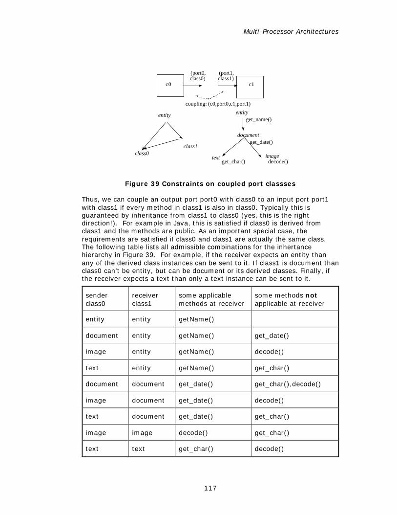
Multi-Processor Architectures
117
(port0,
c1c0
coupling: (c0,port0,c1,port1)
class0)
entity
text
(port1,class1)
entity
class0class1
document
image
get_name()
get_date()
get_char() decode()
Figure 39 Constraints on coupled port classses
Thus, we can couple an output port port0 with class0 to an input port port1 with class1 if every method in class1 is also in class0. Typically this is guaranteed by inheritance from class1 to class0 (yes, this is the right direction!). For example in Java, this is satisfied if class0 is derived from class1 and the methods are public. As an important special case, the requirements are satisfied if class0 and class1 are actually the same class. The following table lists all admissible combinations for the inhertance hierarchy in Figure 39. For example, if the receiver expects an entity than any of the derived class instances can be sent to it. If class1 is document than class0 can’t be entity, but can be document or its derived classes. Finally, if the receiver expects a text than only a text instance can be sent to it.
sender class0
receiver class1
some applicable methods at receiver
some methods not applicable at receiver
entity entity getName()
document entity getName() get_date()
image entity getName() decode()
text entity getName() get_char()
document document get_date() get_char(),decode()
image document get_date() decode()
text document get_date() get_char()
image image decode() get_char()
text text get_char() decode()
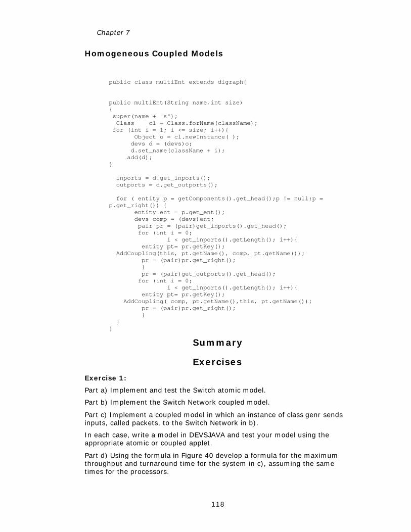
Chapter 7
118
Homogeneous Coupled Models
Summary
Exercises
Exercise 1:
Part a) Implement and test the Switch atomic model.
Part b) Implement the Switch Network coupled model.
Part c) Implement a coupled model in which an instance of class genr sends inputs, called packets, to the Switch Network in b).
In each case, write a model in DEVSJAVA and test your model using the appropriate atomic or coupled applet.
Part d) Using the formula in Figure 40 develop a formula for the maximum throughput and turnaround time for the system in c), assuming the same times for the processors.
public class multiEnt extends digraph{ public multiEnt(String name,int size) { super(name + "s"); Class cl = Class.forName(className); for (int i = 1; i <= size; i++){ Object o = cl.newInstance( ); devs d = (devs)o; d.set_name(className + i); add(d); } inports = d.get_inports(); outports = d.get_outports(); for ( entity p = getComponents().get_head();p != null;p = p.get_right()) { entity ent = p.get_ent(); devs comp = (devs)ent; pair pr = (pair)get_inports().get_head(); for (int i = 0; i < get_inports().getLength(); i++){ entity pt= pr.getKey(); AddCoupling(this, pt.getName(), comp, pt.getName()); pr = (pair)pr.get_right(); } pr = (pair)get_outports().get_head(); for (int i = 0; i < get_inports().getLength(); i++){ entity pt= pr.getKey(); AddCoupling( comp, pt.getName(),this, pt.getName()); pr = (pair)pr.get_right(); } } }
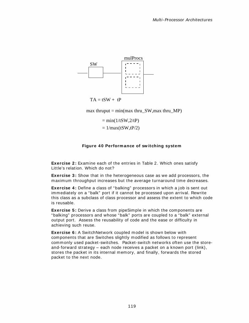
Multi-Processor Architectures
119
max thruput = min(max thru_SW,max thru_MP)
SWmulProcs
= min(1/tSW,2/tP) = 1/max(tSW,tP/2)
TA = tSW + tP
Figure 40 Performance of switching system
Exercise 2: Examine each of the entries in Table 2. Which ones satisfy Little’s relation. Which do not?
Exercise 3: Show that in the heterogeneous case as we add processors, the maximum throughput increases but the average turnaround time decreases.
Exercise 4: Define a class of “balking” processors in which a job is sent out immediately on a “balk” port if it cannot be processed upon arrival. Rewrite this class as a subclass of class processor and assess the extent to which code is reusable.
Exercise 5: Derive a class from pipeSimple in which the components are “balking” processors and whose “balk” ports are coupled to a “balk” external output port. Assess the reusability of code and the ease or difficulty in achieving such reuse.
Exercise 6: A SwitchNetwork coupled model is shown below with components that are Switches slightly modified as follows to represent commonly used packet-switches. Packet-switch networks often use the store-and-forward strategy – each node receives a packet on a known port (link), stores the packet in its internal memory, and finally, forwards the stored packet to the next node.
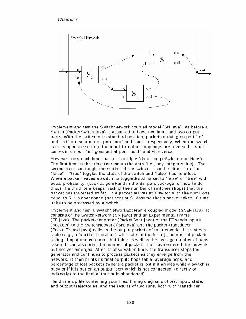
Chapter 7
120
Implement and test the SwitchNetwork coupled model (SN.java). As before a Switch (PacketSwitch.java) is assumed to have two input and two output ports. With the switch in its standard position, packets arriving on port “in” and “in1” are sent out on port “out” and “out1” respectively. When the switch is in its opposite setting, the input-to-output mappings are reversed – what comes in on port “in” goes out at port “out1” and vice versa.
However, now each input packet is a triple (data, toggleSwitch, numHops). The first item in the triple represents the data (i.e., any integer value). The second item can toggle the setting of the switch: it can be either “true” or “false” – “true” toggles the state of the switch and “false” has no effect. When a packet leaves a switch its toggleSwitch is set to “false” or “true” with equal probability. (Look at genrRand in the Simparc package for how to do this.) The third item keeps track of the number of switches (hops) that the packet has traversed so far. If a packet arrives at a switch with the numHops equal to 5 it is abandoned (not sent out). Assume that a packet takes 10 time units to be processed by a switch.
Implement and test a SwitchNetworkExpFrame coupled model (SNEF.java). It consists of the SwitchNetwork (SN.java) and an Experimental Frame (EF.java). The packet-generator (PacketGenr.java) of the EF sends inputs (packets) to the SwitchNetwork (SN.java) and the packet-transducer (PacketTransd.java) collects the output packets of the network. It creates a table (e.g., a function container) with pairs of the form (i, number of packets taking i hops) and can print that table as well as the average number of hops taken. It can also print the number of packets that have entered the network but not yet emerged. After its observation time, the transducer stops the generator and continues to process packets as they emerge from the network. It then prints its final output: hops table, average hops, and percentage of lost packets (where a packet is lost if it arrives while a switch is busy or if it is put on an output port which is not connected (directly or indirectly) to the final output or is abandoned).
Hand in a zip file containing your files, timing diagrams of test input, state, and output trajectories, and the results of two runs, both with transducer
Multi-Processor Architectures
121
observation time equal to 1000. In the first, the generator outputs packets each 10 units; in the second each 5 units. The toggleSwitch item in the triple message output by the generator is set to “false” or “true” with equal probability and is used to set the toggleSwitch setting of the S0 switch.
Solution
Additional Assumptions:
q Generator is assumed to produce new packets with its switch setting equal to false and initial number of hops set to zero.
q PacketSwitch determines whether an incoming packet is to be sent to any other PacketSwitch or not depending on a selected probability setting.
q PacketSwitch can only receive only one input packet and transmitting it to another depending on the input port. Note that Generator produces one packet at a time and PacketSwitch outputs at most one packet at a time.
q All probabilities used are 50% with uniform distribution.
q A packet can take at most 60 units of time (maximum number of hops is 5) before it exists the SwitchNetwork; otherwise it is lost. This upper limit is included to ensure that the last packet entering the SwitchNetwork can be accounted for if indeed it is allowed to exist.
Models:
EF.java
packet.java
PacketGenr.java
PacketTransd.java
PacketSwitch.java
SN.java
SNEF.java
Simulation Results:
Simulation Run #1-1:
Generator:
Produces jobs every 10 units of time
Transducer:
Observation Period: 1060 units of time
packets arrived: 101
packets transmitted: 10
Avg. num. of hops: 3.3
Percentage of packets lost: 90.0%
Chapter 7
122
P3,7
P4,3
P5,0
P2,0
P1,0
Simulation Run #1-2:
Generator:
Produces jobs every 10 units of time
Transducer:
packets arrived: 101
packets transmitted: 7
Avg. num. of hops: 3.7142857142857144
Percentage of packets lost: 93.0%
P4,5
P3,2
P5,0
P2,0
P1,0
Simulation Run #2-1:
Generator:
Produces jobs every 5 units of time
Transducer:
Observation Period: 1060 units of time
packets arrived: 201
packets transmitted: 15
Avg. num. of hops: 3.6666666666666665
Percentage of packets lost: 92.0%
P5,2
P3,7
P4,6
P2,0
P1,0
Simulation Run #2-2:
Generator:
Produces jobs every 5 units of time
Multi-Processor Architectures
123
Transducer:
Observation Period: 1060 units of time
packets arrived: 201
packets transmitted: 12
Avg. num. of hops: 3.25
Percentage of packets lost: 94.0%
P3,10
P4,1
P5,1
P2,0
P1,0
Exercise 7: Consider a real world system in which there are vehicles and their owners and a repair shop employing a single mechanic. The mechanic receives a vehicle for repair from its owner. He gives the customer estimates for repair cost and delivery date. However, halfway through the course of repair, the mechanic may find out that the cost of repair will be greater than he had estimated (e.g., twice the original estimate). In this case, the mechanic will have to notify the client about the additional cost and estimated time to complete the repair. He stops working on the repair. Once the client agrees to pay the higher amount, the repair will continue with a new delivery date. The new delivery date can be sooner or later than the original date. In the following, be sure to give any assumptions you make.
q Suppose the mechanic can only repair one car at a time. That is the mechanic will not start repair of another car until the current repair is completed. Cars that arrive while the mechanic is busy try to come back later or go to another repair shop. Develop an atomic DEVS model (pseudo form or Java code) for this repair shop with timing diagrams depicting key input, output, and state transitions.
q Consider the case where the repair shop employs several mechanics. Consider three repair shop architectures, based on multi-server, pipeline, and divide-and-conquer, by which the shop manager can distribute incoming repair requests (in this case, you can assume the shop manager always gets the estimated time and cost correct the first time). There can be mechanics, which are generalists or specialists. For example, a mechanic’s specialty might be in engine repair or electrical system repair. Also assume that the shop manager first analyzes the car’s problems and writes a repair order that can consist of a number of tasks (e.g., replace fuel control and replace electrical wiring).
For each of the three cases, draw a diagram of the coupled model and provide a paragraph description of how the architecture works (no code or pseudo code is required)
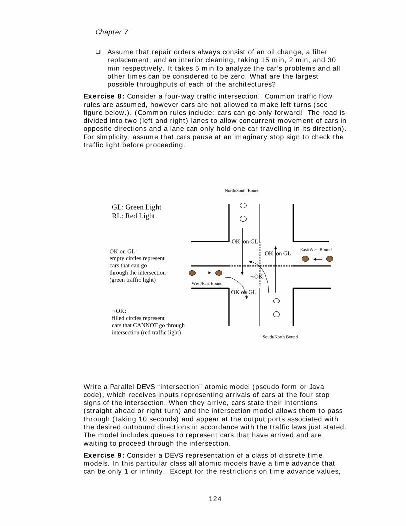
Chapter 7
124
q Assume that repair orders always consist of an oil change, a filter replacement, and an interior cleaning, taking 15 min, 2 min, and 30 min respectively. It takes 5 min to analyze the car’s problems and all other times can be considered to be zero. What are the largest possible throughputs of each of the architectures?
Exercise 8: Consider a four-way traffic intersection. Common traffic flow rules are assumed, however cars are not allowed to make left turns (see figure below.). (Common rules include: cars can go only forward! The road is divided into two (left and right) lanes to allow concurrent movement of cars in opposite directions and a lane can only hold one car travelling in its direction). For simplicity, assume that cars pause at an imaginary stop sign to check the traffic light before proceeding.
OK on GL
¬OK
OK on GL
GL: Green LightRL: Red Light
OK on GLOK on GL: empty circles representcars that can gothrough the intersection (green traffic light)
¬OK:filled circles representcars that CANNOT go through intersection (red traffic light)
East/West Bound
West/East Bound
North/South Bound
South/North Bound
Write a Parallel DEVS “intersection” atomic model (pseudo form or Java code), which receives inputs representing arrivals of cars at the four stop signs of the intersection. When they arrive, cars state their intentions (straight ahead or right turn) and the intersection model allows them to pass through (taking 10 seconds) and appear at the output ports associated with the desired outbound directions in accordance with the traffic laws just stated. The model includes queues to represent cars that have arrived and are waiting to proceed through the intersection.
Exercise 9: Consider a DEVS representation of a class of discrete time models. In this particular class all atomic models have a time advance that can be only 1 or infinity. Except for the restrictions on time advance values,
Multi-Processor Architectures
125
such models follow the usual parallel DEVS conventions. In particular they can produce output messages, which may or may not be null. In a coupled model containing these models as components, the normal coupling rules apply so that components can get inputs from a subset (possibly empty) of other components. We’ll restrict attention to coupled models that have no external input ports and which initialize their components so that their elapsed times are zero.
q An example of such an atomic model is the following. It can receive any number of real valued inputs on its input port “in”. No matter what its current state is, when it receives a bag of such inputs, it takes their average. If the average is less than 1, it passivates. Otherwise, it outputs the average after 1 time unit on port “out”, and if no input is received at that time, it passivates. In either mathematical form or pseudo code, write a parallel atomic DEVS model for this example.
q Using the standard Parallel DEVS simulation protocol, describe the exact conditions under which the internal, external and confluent transition functions of the components are applied in a simulations of coupled models with components described in a).
q Consider coupled models of components of the discrete time class described above (of which those in a) are special cases). Assume the number of components is very large and the maximum number of influencees of any component (the possible receivers of its output) is very much smaller. Develop an optimization of the standard Parallel DEVS simulation protocol that allows the coordinator to use its knowledge of the restricted time advances and the model coupling information to reduce the number of messages it exchanges with the simulators of the components. Your algorithms for coordinator and simulator can be given in any convenient form. Explain where your version provides the savings in messages in comparison to the standard protocol.
Solution
5b) Conditions under which the transition functions are applied.
The “status” of any discrete time model in state s can be defined as follows:
“active” if ta(s) = 1 “passive” if ta(s) = infinity.
Note that “status” can always be defined independently of what the phase is.
Now if the “status” is “passive” and input is not null then apply external transition fn
if the “status” is “active” and input is null then apply internal transition fn
if the “status” is “active” and input is not null then apply confluent transition fn
Chapter 7
126
5c) Parallel DEVS Protocol for discrete time models
Coordinator sends nextTN to request tN from each of the simulators.
All the simulators reply with their tNs in the outTN message to the coordinator
Coordinator sets activeList = {simulators for which tN = 1} (these are the imminents)
Coordinator sends to each simulator in activeList a getOut message and waits for all outputs to return
Coordinator extends activeList by including all influencees of members already in activeList (obtained from coupling)
Coordinator uses the coupling specification to distribute the outputs as inputs in an applyDelt message to the simulators in the activeList
Coordinator waits for all simulators in activeList to return with their next outputs
Coordinator sets activeList = {simulators for which output is not null}(these are the imminents)
If activeList is not empty, Coordinator passivates, else goes to step 5.
Comments:
q The only time the coordinator needs to get tNs from the simulators is initially (to determine the initial imminents). Here we save on nextTN and outTN messages each cycle
q The only time the coordinator needs to send a getOut message is initially to get the outputs from the imminents. Here we save on getOut messages each cycle.
q Once it knows the outputs of the imminents, the coordinator can determine their influencees and what they should receive as input (using the coupling). This adds to the activeList in step 5.
q We still need an applyDelt message containing input each cycle but this needs to be sent only to the activeList – by what’s given in the problem statement, the activeList should always be quite small relative to the full set of components
q We modify the simulator’s response to an applyDelt so that it returns its model’s next output – after its applyDelt, a simulator will either be passive (have tN = infinity) or active (tN = tN +1); if it is active it can go ahead and compute the models next output.
The messages required after the initial setup cycle are:
Coordinator sends applyDelt to the activeList
Simulators in activeList send output in response to applyDelt
To reduce such messaging, the coordinator needs to maintain the activeList – which it does not need to do in the standard protocol.
Multi-Processor Architectures
127
Exercise 10: Consider Divide&Conquer architecture discussed in lecture and described in the text. Suppose three processors P1, P2, P3 are available to process three pieces (job1,p1, job1,p2, and job1,p3) of an incoming job (job1).
(a) Extend the Divide&Conquer model (call it D&Cext) so that it breaks an incoming job (jobj, unsolved) into parts (jobj,p1, jobj,p2, and jobj,p3) and assembles them upon their completion (jobj, solved). Assume some none-zero processing time (td) is required to break a job into parts and similarly some none-zero processing time is needed (ta) to assemble the individually solved pieces together. Specify D&Cext model (i.e., determine all components (parent and children) and couplings). You can draw the D&Cext digraph model – that is draw components, ports, and couplings and specify their names. Alternatively, you may use mathematical or pseudo notation.
(b) Determine theoretical turn around time and throughput for D&Cext architecture assuming incoming jobs can be equally divided into three pieces and the three P1, P2, and P3 can process their jobs using exactly the same time period.
(c) Determine whether it is possible for D&Cext model to have worse turn around time and/or worse throughput compared with a single processor. Explain and quantify your answer.
Exercise 11: Consider a real world system in which there are vehicles and their owners and a repair shop employing a single mechanic. The mechanic receives a vehicle for repair from its owner. He gives the customer estimates for repair cost and delivery date. However, halfway through the course of repair, the mechanic may find out that the cost of repair will be greater than he had estimated (e.g., twice the original estimate). In this case, the mechanic will have to notify the client about the additional cost and estimated time to complete the repair. He stops working on the repair. Once the client agrees to pay the higher amount, the repair will continue with a new delivery date. The new delivery date can be sooner or later than the original date. In the following, be sure to give any assumptions you make.
Suppose the mechanic can only repair one car at a time. That is the mechanic will not start repair of another car until the current repair is completed. Cars that arrive while the mechanic is busy try to come back later or go to another repair shop. Develop an atomic DEVS model (pseudo form or Java code) for this repair shop with timing diagrams depicting key input, output, and state transitions.
Consider the case where the repair shop employs several mechanics. Consider three repair shop architectures, based on multi-server, pipeline, and divide-and-conquer, by which the shop manager can distribute incoming repair requests (in this case, you can assume the shop manager always gets the estimated time and cost correct the first time). There can be mechanics which are generalists or specialists. For example, a mechanic’s specialty might be in engine repair or electrical system repair. Also assume that the shop manager first analyzes the car’s problems and writes a repair order that can consist of a number of tasks (e.g., replace fuel control and replace electrical wiring).
For each of the three cases, draw a diagram of the coupled model and provide a paragraph description of how the architecture works (no code or pseudo code is required)

Chapter 7
128
Assume that repair orders always consist of an oil change, a filter replacement, and an interior cleaning, taking 15 min, 2 min, and 30 min respectively. It takes 5 min to analyze the car’s problems and all other times can be considered to be zero. What are the largest possible throughputs of each of the architectures?
Chapter 8
SYSTEM ENTITY STRUCTURE
Simulation-based systems design employs a plan-generate-evaluate process. The plan phase organizes all the models of design alternatives within the chosen system boundary and design objectives. The generate phase synthesizes a candidate design model intended to meet the set of design objectives. Finally, the evaluate phase evaluates behavior and/or performance of the generated model through simulation using an appropriate experimental frame derived from the design objectives. The overall design cycle repeats the generation and evaluation phases until an acceptable design is found.
How can we organize a family of candidate models from which a candidate model can be selected, generated and evaluated? This chapter presents the systems entity structure/model base (SES/MB) framework for such an organization. The idea is as follows. Let us first extract the hierarchical composition structures of hierarchical, modular models from their implementations. Then we save the structures and the implementations separately in organized libraries. 0 shows the basic idea in which libraries for model structures and model implementations are called system entity structure base and model base, respectively. Our goal is to be able to synthesize a simulation model by traversing a model hierarchical structure, retrieving component implementations and coupling them together. As will be seen later in this chapter, a system entity structure represents not a single model structure, but a family of model structures, from which a candidate structure called a pruned entity structure can be selected. Thus, the system-entity-structure/model-base framework supports the plan-generate-evaluate process in systems design.
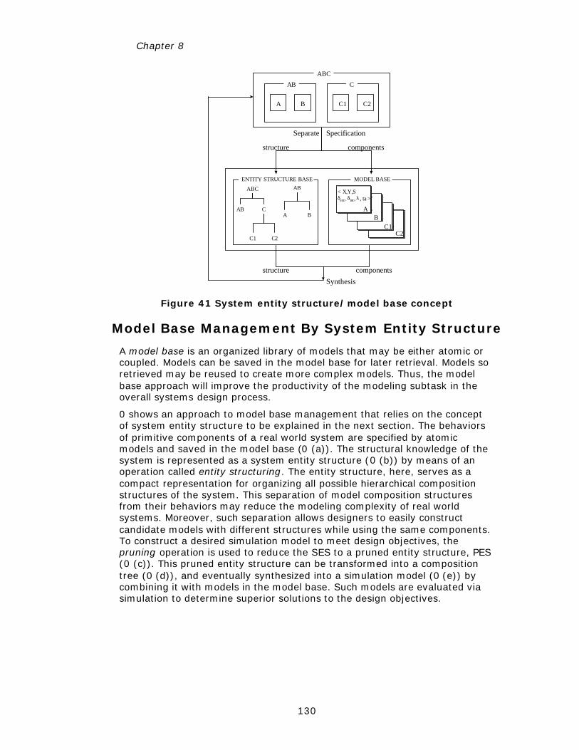
Chapter 8
130
ENTITY STRUCTURE BASE MODEL BASE
ABC
AB C
C2C1
AB
A B
A B C1 C2
ABC
CAB
Specification
Synthesis
components structure
…………
C2C1
…………
BA
< X,Y,Sδext, δint, λ, ta >
structure components
Separate
Figure 41 System entity structure/model base concept
Model Base Management By System Entity Structure
A model base is an organized library of models that may be either atomic or coupled. Models can be saved in the model base for later retrieval. Models so retrieved may be reused to create more complex models. Thus, the model base approach will improve the productivity of the modeling subtask in the overall systems design process.
0 shows an approach to model base management that relies on the concept of system entity structure to be explained in the next section. The behaviors of primitive components of a real world system are specified by atomic models and saved in the model base (0 (a)). The structural knowledge of the system is represented as a system entity structure (0 (b)) by means of an operation called entity structuring. The entity structure, here, serves as a compact representation for organizing all possible hierarchical composition structures of the system. This separation of model composition structures from their behaviors may reduce the modeling complexity of real world systems. Moreover, such separation allows designers to easily construct candidate models with different structures while using the same components. To construct a desired simulation model to meet design objectives, the pruning operation is used to reduce the SES to a pruned entity structure, PES (0 (c)). This pruned entity structure can be transformed into a composition tree (0 (d)), and eventually synthesized into a simulation model (0 (e)) by combining it with models in the model base. Such models are evaluated via simulation to determine superior solutions to the design objectives.
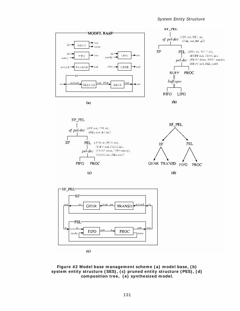
System Entity Structure
131
Figure 42 Model base management scheme (a) model base, (b) system entity structure (SES), (c) pruned entity structure (PES), (d)
composition tree, (e) synthesized model.
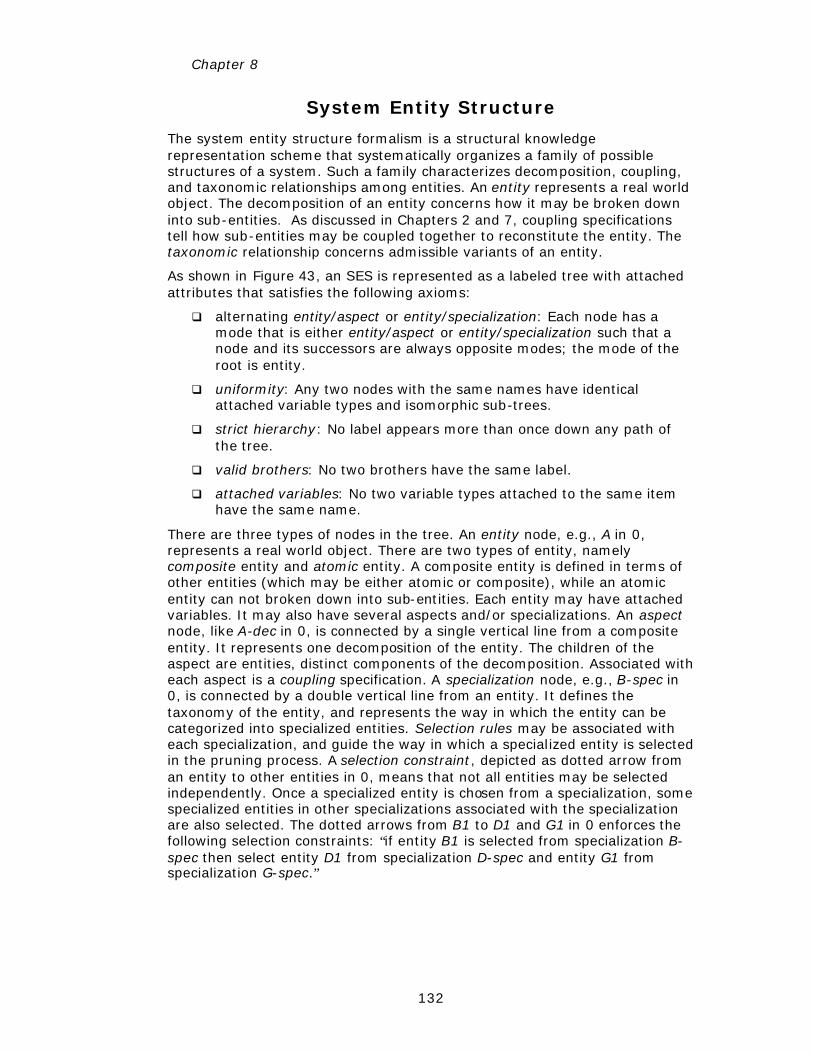
Chapter 8
132
System Entity Structure
The system entity structure formalism is a structural knowledge representation scheme that systematically organizes a family of possible structures of a system. Such a family characterizes decomposition, coupling, and taxonomic relationships among entities. An entity represents a real world object. The decomposition of an entity concerns how it may be broken down into sub-entities. As discussed in Chapters 2 and 7, coupling specifications tell how sub-entities may be coupled together to reconstitute the entity. The taxonomic relationship concerns admissible variants of an entity.
As shown in Figure 43, an SES is represented as a labeled tree with attached attributes that satisfies the following axioms:
q alternating entity/aspect or entity/specialization: Each node has a mode that is either entity/aspect or entity/specialization such that a node and its successors are always opposite modes; the mode of the root is entity.
q uniformity: Any two nodes with the same names have identical attached variable types and isomorphic sub-trees.
q strict hierarchy: No label appears more than once down any path of the tree.
q valid brothers: No two brothers have the same label.
q attached variables: No two variable types attached to the same item have the same name.
There are three types of nodes in the tree. An entity node, e.g., A in 0, represents a real world object. There are two types of entity, namely composite entity and atomic entity. A composite entity is defined in terms of other entities (which may be either atomic or composite), while an atomic entity can not broken down into sub-entities. Each entity may have attached variables. It may also have several aspects and/or specializations. An aspect node, like A-dec in 0, is connected by a single vertical line from a composite entity. It represents one decomposition of the entity. The children of the aspect are entities, distinct components of the decomposition. Associated with each aspect is a coupling specification. A specialization node, e.g., B-spec in 0, is connected by a double vertical line from an entity. It defines the taxonomy of the entity, and represents the way in which the entity can be categorized into specialized entities. Selection rules may be associated with each specialization, and guide the way in which a specialized entity is selected in the pruning process. A selection constraint, depicted as dotted arrow from an entity to other entities in 0, means that not all entities may be selected independently. Once a specialized entity is chosen from a specialization, some specialized entities in other specializations associated with the specialization are also selected. The dotted arrows from B1 to D1 and G1 in 0 enforces the following selection constraints: “if entity B1 is selected from specialization B-spec then select entity D1 from specialization D-spec and entity G1 from specialization G-spec.”
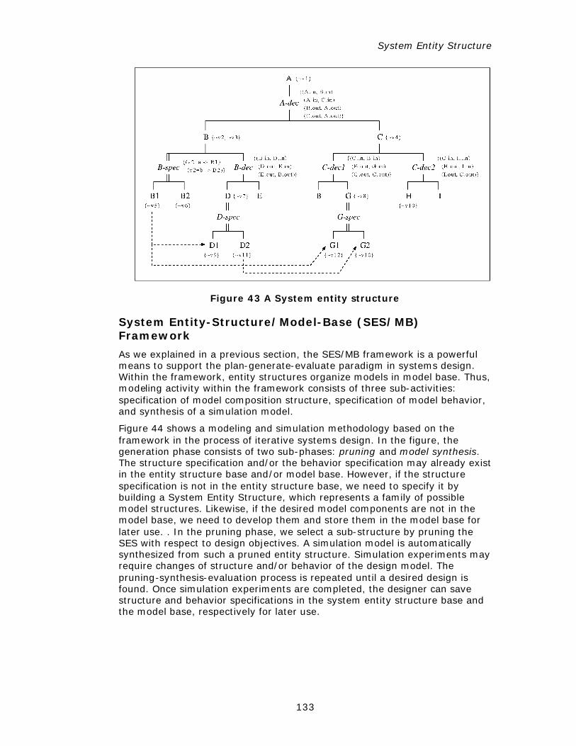
System Entity Structure
133
Figure 43 A System entity structure
System Entity-Structure/Model-Base (SES/MB) Framework
As we explained in a previous section, the SES/MB framework is a powerful means to support the plan-generate-evaluate paradigm in systems design. Within the framework, entity structures organize models in model base. Thus, modeling activity within the framework consists of three sub-activities: specification of model composition structure, specification of model behavior, and synthesis of a simulation model.
Figure 44 shows a modeling and simulation methodology based on the framework in the process of iterative systems design. In the figure, the generation phase consists of two sub-phases: pruning and model synthesis. The structure specification and/or the behavior specification may already exist in the entity structure base and/or model base. However, if the structure specification is not in the entity structure base, we need to specify it by building a System Entity Structure, which represents a family of possible model structures. Likewise, if the desired model components are not in the model base, we need to develop them and store them in the model base for later use. . In the pruning phase, we select a sub-structure by pruning the SES with respect to design objectives. A simulation model is automatically synthesized from such a pruned entity structure. Simulation experiments may require changes of structure and/or behavior of the design model. The pruning-synthesis-evaluation process is repeated until a desired design is found. Once simulation experiments are completed, the designer can save structure and behavior specifications in the system entity structure base and the model base, respectively for later use.
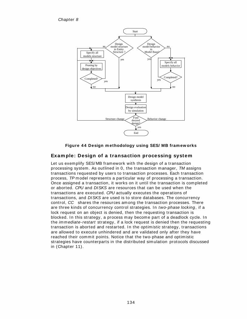
Chapter 8
134
Start
Design model structure
in Entity Structure ?
Designmodel behavior
in Model Base?Specify all
models structure
Pruning bydesign objectives
Completed?
Specify allmodels behavior
Completed?
Design evaluationby simulation
Design modelsynthesis
no
yes
no
no
no
yes yes
yes
Finddesireddesign?
Structure change Behavior change
yes
End
Figure 44 Design methodology using SES/MB frameworks
Example: Design of a transaction processing system
Let us exemplify SES/MB framework with the design of a transaction processing system. As outlined in 0, the transaction manager, TM assigns transactions requested by users to transaction processes. Each transaction process, TP model represents a particular way of processing a transaction. Once assigned a transaction, it works on it until the transaction is completed or aborted. CPU and DISKS are resources that can be used when the transactions are executed. CPU actually executes the operations of transactions, and DISKS are used is to store databases. The concurrency control, CC shares the resources among the transaction processes. There are three kinds of concurrency control strategies. In two-phase locking, if a lock request on an object is denied, then the requesting transaction is blocked. In this strategy, a process may become part of a deadlock cycle. In the immediate-restart strategy, if a lock request is denied then the requesting transaction is aborted and restarted. In the optimistic strategy, transactions are allowed to execute unhindered and are validated only after they have reached their commit points. Notice that the two-phase and optimistic strategies have counterparts in the distributed simulation protocols discussed in (Chapter 11).
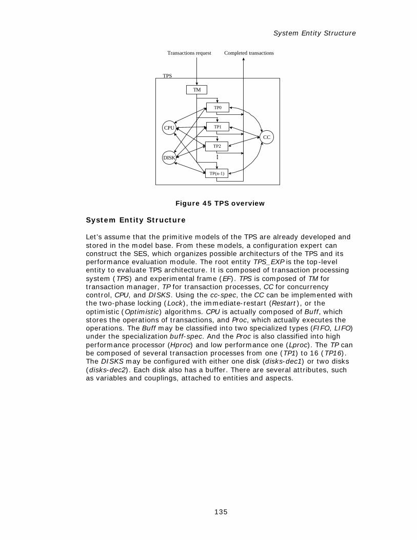
System Entity Structure
135
Transactions request
CPU
DISK
CC
TM
TP0
TP1
TP2
TP(n-1)
TPS
...
Completed transactions
Figure 45 TPS overview
System Entity Structure
Let’s assume that the primitive models of the TPS are already developed and stored in the model base. From these models, a configuration expert can construct the SES, which organizes possible architecturs of the TPS and its performance evaluation module. The root entity TPS_EXP is the top-level entity to evaluate TPS architecture. It is composed of transaction processing system (TPS) and experimental frame (EF). TPS is composed of TM for transaction manager, TP for transaction processes, CC for concurrency control, CPU, and DISKS. Using the cc-spec, the CC can be implemented with the two-phase locking (Lock), the immediate-restart (Restart), or the optimistic (Optimistic) algorithms. CPU is actually composed of Buff, which stores the operations of transactions, and Proc, which actually executes the operations. The Buff may be classified into two specialized types (FIFO, LIFO) under the specialization buff-spec. And the Proc is also classified into high performance processor (Hproc) and low performance one (Lproc). The TP can be composed of several transaction processes from one (TP1) to 16 (TP16). The DISKS may be configured with either one disk (disks-dec1) or two disks (disks-dec2). Each disk also has a buffer. There are several attributes, such as variables and couplings, attached to entities and aspects.
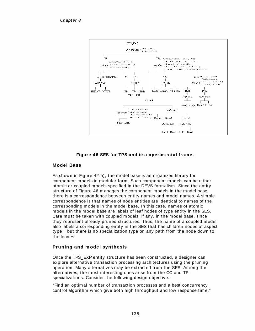
Chapter 8
136
Figure 46 SES for TPS and its experimental frame.
Model Base
As shown in Figure 42 a), the model base is an organized library for component models in modular form. Such component models can be either atomic or coupled models specified in the DEVS formalism. Since the entity structure of Figure 46 manages the component models in the model base, there is a correspondence between entity names and model names. A simple correspondence is that names of node entities are identical to names of the corresponding models in the model base. In this case, names of atomic models in the model base are labels of leaf nodes of type entity in the SES. Care must be taken with coupled models, if any, in the model base, since they represent already pruned structures. Thus, the name of a coupled model also labels a corresponding entity in the SES that has children nodes of aspect type − but there is no specialization type on any path from the node down to the leaves.
Pruning and model synthesis
Once the TPS_EXP entity structure has been constructed, a designer can explore alternative transaction processing architectures using the pruning operation. Many alternatives may be extracted from the SES. Among the alternatives, the most interesting ones arise from the CC and TP specializations. Consider the following design objective:
“Find an optimal number of transaction processes and a best concurrency control algorithm which give both high throughput and low response time.”
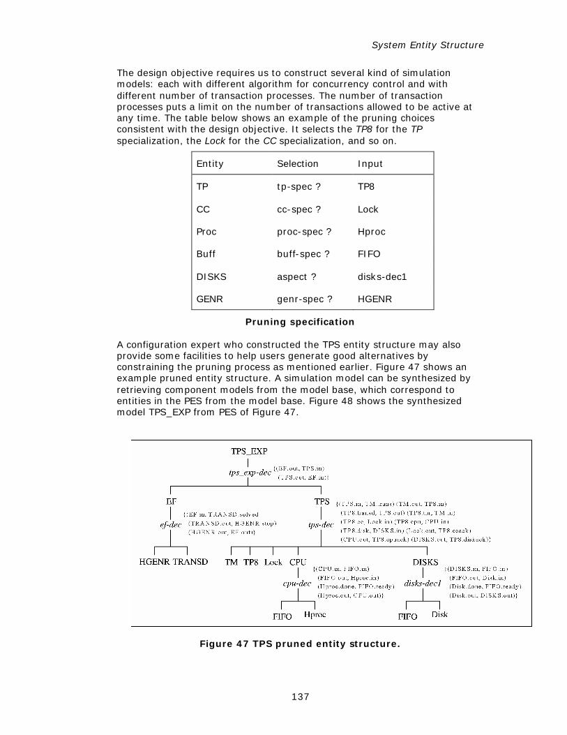
System Entity Structure
137
The design objective requires us to construct several kind of simulation models: each with different algorithm for concurrency control and with different number of transaction processes. The number of transaction processes puts a limit on the number of transactions allowed to be active at any time. The table below shows an example of the pruning choices consistent with the design objective. It selects the TP8 for the TP specialization, the Lock for the CC specialization, and so on.
Entity Selection Input
TP tp-spec ? TP8
CC cc-spec ? Lock
Proc proc-spec ? Hproc
Buff buff-spec ? FIFO
DISKS aspect ? disks-dec1
GENR genr-spec ? HGENR
Pruning specification
A configuration expert who constructed the TPS entity structure may also provide some facilities to help users generate good alternatives by constraining the pruning process as mentioned earlier. Figure 47 shows an example pruned entity structure. A simulation model can be synthesized by retrieving component models from the model base, which correspond to entities in the PES from the model base. Figure 48 shows the synthesized model TPS_EXP from PES of Figure 47.
Figure 47 TPS pruned entity structure.
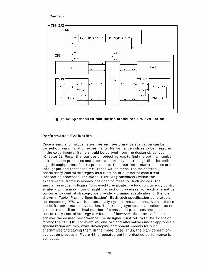
Chapter 8
138
Figure 48 Synthesized simulation model for TPS evaluation.
Performance Evaluation
Once a simulation model is synthesized, performance evaluation can be carried out via simulation experiments. Performance indices to be measured in the experimental frame should be derived from the design objectives (Chapter 2). Recall that our design objective was to find the optimal number of transaction processes and a best concurrency control algorithm for both high throughput and fast response time. Thus, our performance indices are throughput and response time. These will be measured for different concurrency control strategies as a function of number of concurrent transaction processes. The model TRANSD (transducer) within the experimental frame is already designed to measure such indices. The simulation model in Figure 48 is used to evaluate the lock concurrency control strategy with a maximum of eight transaction processes. For each alternative concurrency control strategy, we provide a pruning specification of the form shown in Table “Pruning Specification”. Each such specification generates a corresponding PES, which automatically synthesizes an alternative simulation model for performance evaluation. The pruning-synthesis-evaluation process is repeated until an optimal number of transaction processes and a best concurrency control strategy are found. If however, the process fails to achieve the desired performance, the designer must return to the extent or modify the SES/MB. For example, one can add alternatives under appropriate specialization entities, while developing component models for such alternatives and saving them in the model base. Thus, the plan-generation-evaluation process in Figure 48 is repeated until the desired performance is achieved.
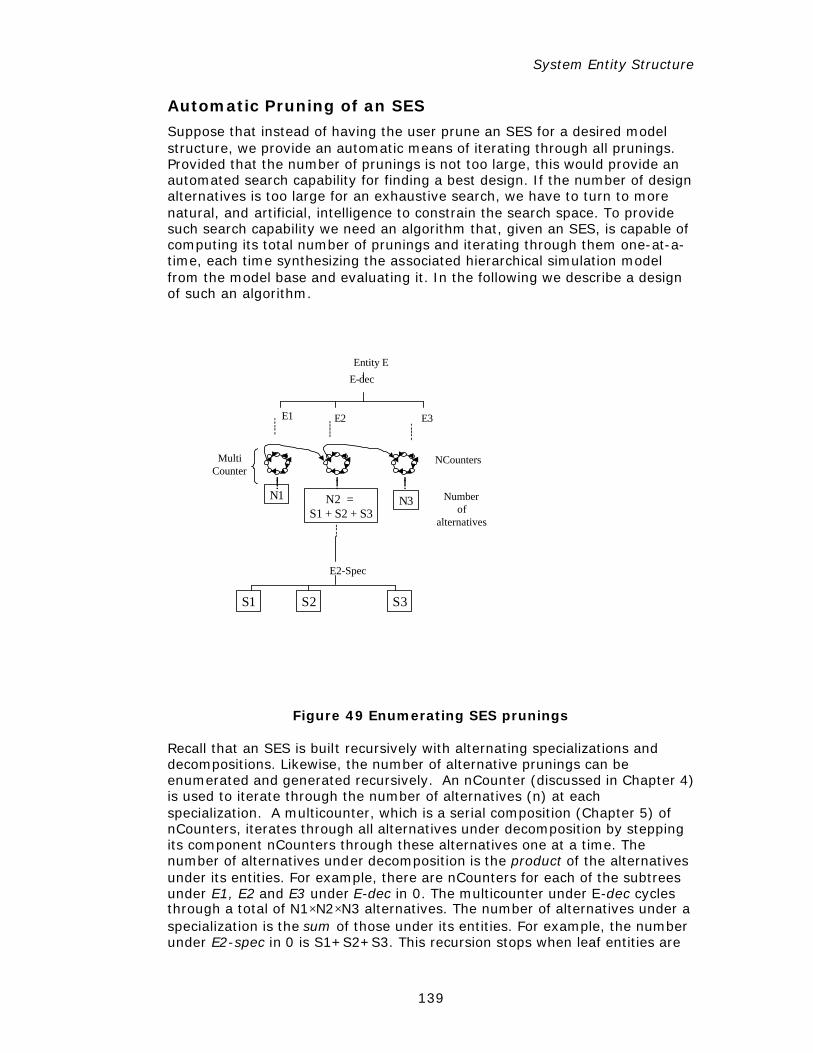
System Entity Structure
139
Automatic Pruning of an SES
Suppose that instead of having the user prune an SES for a desired model structure, we provide an automatic means of iterating through all prunings. Provided that the number of prunings is not too large, this would provide an automated search capability for finding a best design. If the number of design alternatives is too large for an exhaustive search, we have to turn to more natural, and artificial, intelligence to constrain the search space. To provide such search capability we need an algorithm that, given an SES, is capable of computing its total number of prunings and iterating through them one-at-a-time, each time synthesizing the associated hierarchical simulation model from the model base and evaluating it. In the following we describe a design of such an algorithm.
N1 Numberof
alternatives
NCountersMultiCounter
N2 = S1 + S2 + S3
N3
E-dec
S1 S2 S3
Entity E
E1 E2 E3
E2-Spec
Figure 49 Enumerating SES prunings
Recall that an SES is built recursively with alternating specializations and decompositions. Likewise, the number of alternative prunings can be enumerated and generated recursively. An nCounter (discussed in Chapter 4) is used to iterate through the number of alternatives (n) at each specialization. A multicounter, which is a serial composition (Chapter 5) of nCounters, iterates through all alternatives under decomposition by stepping its component nCounters through these alternatives one at a time. The number of alternatives under decomposition is the product of the alternatives under its entities. For example, there are nCounters for each of the subtrees under E1, E2 and E3 under E-dec in 0. The multicounter under E-dec cycles through a total of N1×N2×N3 alternatives. The number of alternatives under a specialization is the sum of those under its entities. For example, the number under E2-spec in 0 is S1+S2+S3. This recursion stops when leaf entities are
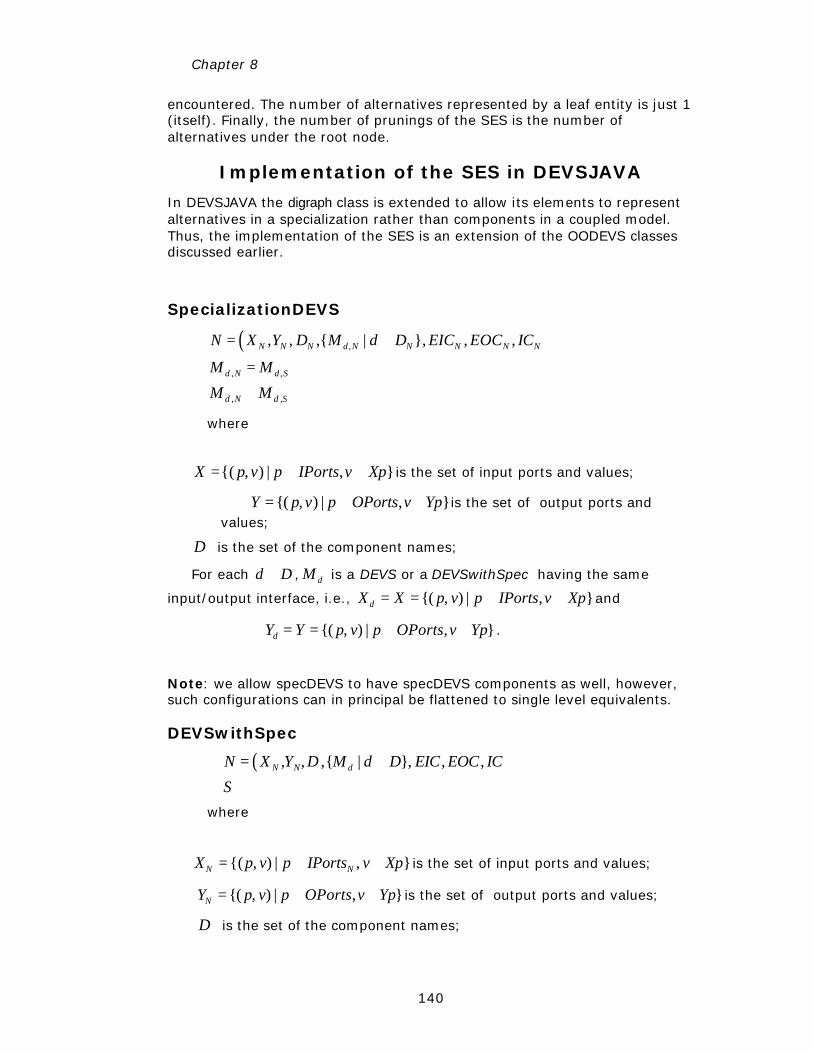
Chapter 8
140
encountered. The number of alternatives represented by a leaf entity is just 1 (itself). Finally, the number of prunings of the SES is the number of alternatives under the root node.
Implementation of the SES in DEVSJAVA
In DEVSJAVA the digraph class is extended to allow its elements to represent alternatives in a specialization rather than components in a coupled model. Thus, the implementation of the SES is an extension of the OODEVS classes discussed earlier.
SpecializationDEVS
( ),
, ,
, ,
, , ,{ | }, , ,N N N d N N N N N
d N d S
d N d S
N X Y D M d D EIC EOC IC
M M
M M
= ∈
=
∈
where
{( , ) | , }X p v p IPorts v Xp= ∈ ∈ is the set of input ports and values;
{( , ) | , }Y p v p OPorts v Yp= ∈ ∈ is the set of output ports and values;
D is the set of the component names;
For each d D∈ , dM is a DEVS or a DEVSwithSpec having the same
input/output interface, i.e., {( , ) | , }dX X p v p IPorts v Xp= = ∈ ∈ and
{( , ) | , }dY Y p v p OPorts v Yp= = ∈ ∈ .
Note: we allow specDEVS to have specDEVS components as well, however, such configurations can in principal be flattened to single level equivalents.
DEVSwithSpec
( ), , ,{ | }, , ,N N dN X Y D M d D EIC EOC IC
S
= ∈
where
{( , ) | , }N NX p v p IPorts v Xp= ∈ ∈ is the set of input ports and values;
{( , ) | , }NY p v p OPorts v Yp= ∈ ∈ is the set of output ports and values;
D is the set of the component names;
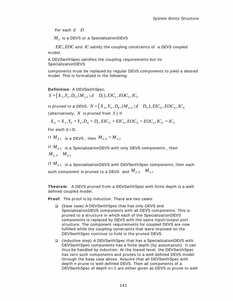
System Entity Structure
141
For each d D∈
dM is a DEVS or a SpecializationDEVS
,EIC EOC and IC satisfy the coupling constraints of a DEVS coupled model.
A DEVSwithSpec satisfies the coupling requirements but its SpecializationDEVS
components must be replaced by regular DEVS components to yield a desired model. This is formalized in the following:
Definition: A DEVSwithSpec,
( ),, , ,{ | }, , ,S S S d S S S S SS X Y D M d D EIC EOC IC= ∈
is pruned to a DEVS, ( ),, , ,{ | }, , ,N N N d N N N N NN X Y D M d D EIC EOC IC= ∈
(alternatively, N is pruned from S ) if
, , , , ,N S N S N S N S N S N SX X Y Y D D EIC EIC EOC EOC IC IC= = = = = =
For each d ε D,
If ,d SM is a DEVS , then , ,d N d SM M=
If ,d SM is a SpecializationDEVS with only DEVS components , then
, ,d N d SM M∈
If ,d SM is a SpecializationDEVS with DEVSwithSpec components, then each
such component is pruned to a DEVS and , ,d N d SM M∈
Theorem: A DEVS pruned from a DEVSwithSpec with finite depth is a well-defined coupled model.
Proof: The proof is by induction. There are two cases:
q (base case) A DEVSwithSpec that has only DEVS and SpecializationDEVS components with all DEVS components. This is pruned to a structure in which each of the SpecializationDEVS components is replaced by DEVS with the same input/output port structure. The component requirements for coupled DEVS are now fulfilled while the coupling constraints that were imposed on the DEVSwithSpec continue to hold in the pruned DEVS.
q (inductive step) A DEVSwithSpec that has a SpecializationDEVS with DEVSwithSpec components has a finite depth (by assumption). It can thus be handled by induction. At the lowest level, the DEVSwithSpec has zero such components and prunes to a well-defined DEVS model through the base case above. Assume that all DEVSwithSpec with depth n prune to well-defined DEVS. Then all components of a DEVSwithSpec of depth n+1 are either given as DEVS or prune to well-
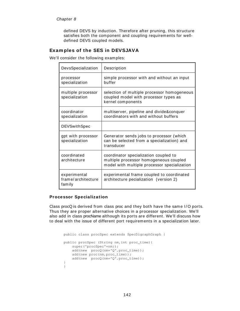
Chapter 8
142
defined DEVS by induction. Therefore after pruning, this structure satisfies both the component and coupling requirements for well-defined DEVS coupled models.
Examples of the SES in DEVSJAVA
We’ll consider the following examples:
DevsSpecialization Description
processor specialization
simple processor with and without an input buffer
multiple processor specialization
selection of multiple processor homogeneous coupled model with processor types as kernel components
coordinator specialization
multiserver, pipeline and divide&conquer coordinators with and without buffers
DEVSwithSpec
gpt with processor specialization
Generator sends jobs to processor (which can be selected from a specialization) and transducer
coordinated architecture
coordinator specialization coupled to multiple processor homogeneous coupled model with multiple processor specialization
experimental frame/architecture family
experimental frame coupled to coordinated architecture pecialization (version 2)
Processor Specialization
Class procQ is derived from class proc and they both have the same I/O ports. Thus they are proper alternative choices in a processor specialization. We’ll also add in class procName although its ports are different. We’ll discuss how to deal with the issue of different port requirements in a specialization later.
public class procSpec extends SpecDigraphGraph { public procSpec (String nm,int proc_time){ super("procSpec"+nm;); add(new procQ(nm+"Q",proc_time)); add(new proc(nm,proc_time)); add(new procQ(nm+"Q",proc_time)); } }
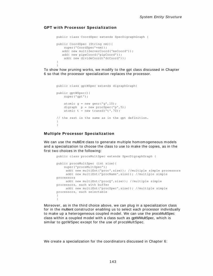
System Entity Structure
143
GPT with Processor Specialization
To show how pruning works, we modify to the gpt class discussed in Chapter 6 so that the processor specialization replaces the processor.
public class gptWSpec extends digraphGraph{ public gptWSpec(){ super("gpt"); atomic g = new genr("g",10); digraph p = new procSpec("p",5); atomic t = new transd("t",70); // the rest is the same as in the gpt definition. } }
Multiple Processor Specialization
We can use the multiEnt class to generate multiple homomogeneous models and a specialization to choose the class to use to make the copies, as in the first two choices in the following:
public class procsMultSpec extends SpecDigraphGraph { public procsMultSpec (int size){ super("procsMultSpec"); add( new multiEnt("proc",size)); //multiple simple processors add( new multiEnt("procName",size)); //multiple simple processors add( new multiEnt("procQ",size)); //multiple simple processors, each with buffer add( new multiEnt("procSpec",size)); //multiple simple processors, each selectable } }
Moreover, as in the third choice above, we can plug in a specialization class for in the multient constructor enabling us to select each processor individually to make up a heterogeneous coupled model. We can use the procsMultSpec class within a coupled model with a class such as gptWMultSpec, which is similar to gptWSpec except for the use of procsMultSpec.
We create a specialization for the coordinators discussed in Chapter 6:
public class CoordSpec extends SpecDigraphGraph { public CoordSpec (String nm)){ super("CoordSpec"+nm)); add( new multiServerCoord("msCoord")); add( new pipeCoord("pipCoord")); add( new divideCoord("dcCoord")); } }
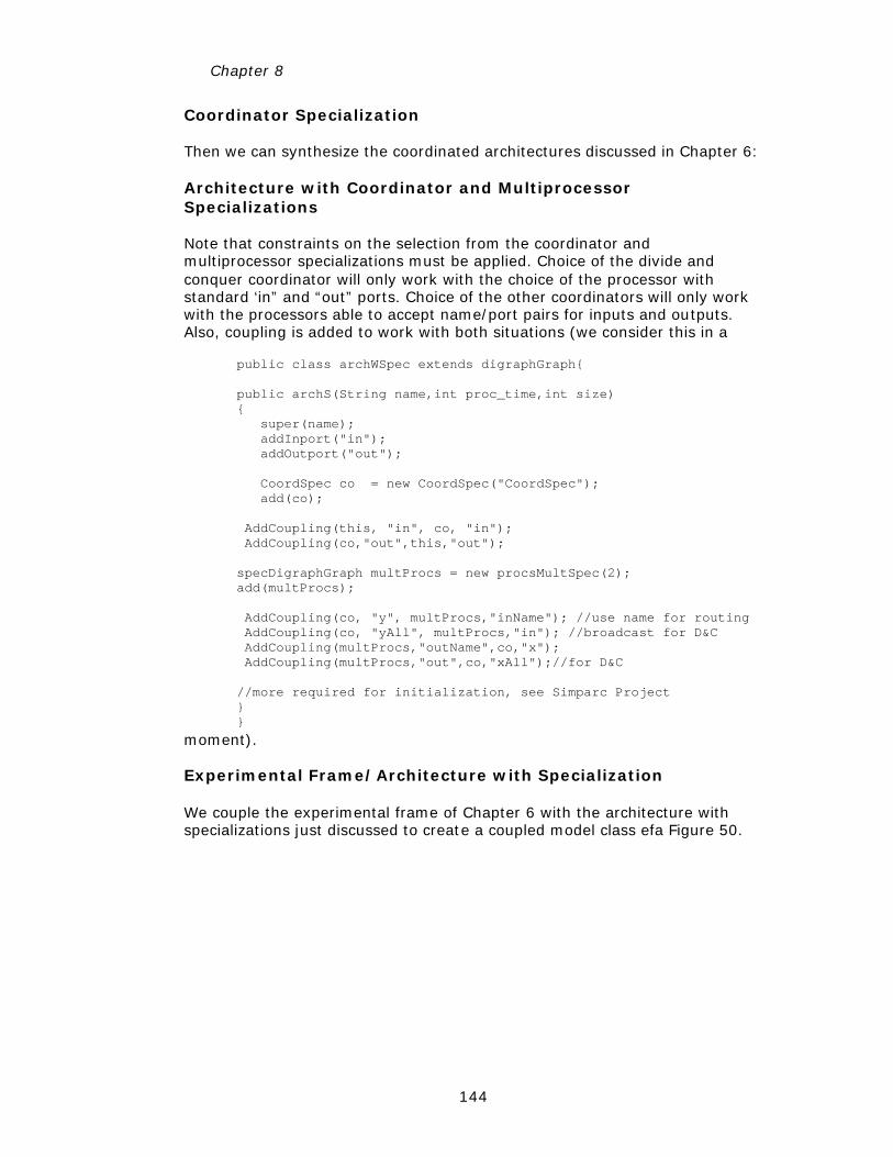
Chapter 8
144
Coordinator Specialization
Then we can synthesize the coordinated architectures discussed in Chapter 6:
Architecture with Coordinator and Multiprocessor Specializations
Note that constraints on the selection from the coordinator and multiprocessor specializations must be applied. Choice of the divide and conquer coordinator will only work with the choice of the processor with standard ‘in” and “out” ports. Choice of the other coordinators will only work with the processors able to accept name/port pairs for inputs and outputs. Also, coupling is added to work with both situations (we consider this in a
moment).
Experimental Frame/Architecture with Specialization
We couple the experimental frame of Chapter 6 with the architecture with specializations just discussed to create a coupled model class efa Figure 50.
public class archWSpec extends digraphGraph{ public archS(String name,int proc_time,int size) { super(name); addInport("in"); addOutport("out"); CoordSpec co = new CoordSpec("CoordSpec"); add(co); AddCoupling(this, "in", co, "in"); AddCoupling(co,"out",this,"out"); specDigraphGraph multProcs = new procsMultSpec(2); add(multProcs); AddCoupling(co, "y", multProcs,"inName"); //use name for routing AddCoupling(co, "yAll", multProcs,"in"); //broadcast for D&C AddCoupling(multProcs,"outName",co,"x"); AddCoupling(multProcs,"out",co,"xAll");//for D&C //more required for initialization, see Simparc Project } }
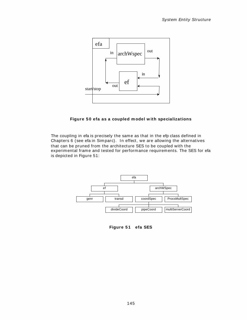
System Entity Structure
145
out
in
archWspec
ef
in
outstart/stop
efa
Figure 50 efa as a coupled model with specializations
The coupling in efa is precisely the same as that in the efp class defined in Chapters 6 (see efa in Simparc). In effect, we are allowing the alternatives that can be pruned from the architecture SES to be coupled with the experimental frame and tested for performance requirements. The SES for efa is depicted in Figure 51:
genr transd
ef
divideCoord pipeCoord multiServerCoord
coordSpec ProcsMultSpec
archWSpec
efa
Figure 51 efa SES
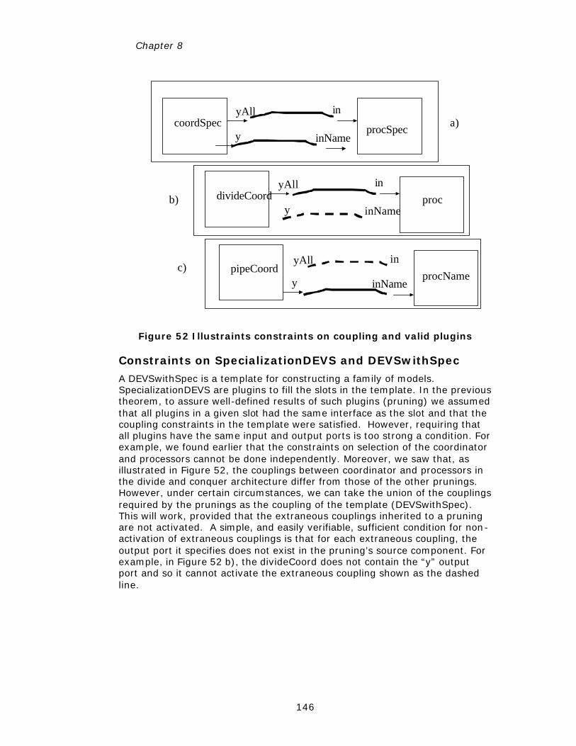
Chapter 8
146
yAll in
y inNamecoordSpec procSpec
yAll individeCoord proc
y inNamepipeCoord
procName
a)
b)
c)
y inName
yAll in
Figure 52 Illustraints constraints on coupling and valid plugins
Constraints on SpecializationDEVS and DEVSwithSpec
A DEVSwithSpec is a template for constructing a family of models. SpecializationDEVS are plugins to fill the slots in the template. In the previous theorem, to assure well-defined results of such plugins (pruning) we assumed that all plugins in a given slot had the same interface as the slot and that the coupling constraints in the template were satisfied. However, requiring that all plugins have the same input and output ports is too strong a condition. For example, we found earlier that the constraints on selection of the coordinator and processors cannot be done independently. Moreover, we saw that, as illustrated in Figure 52, the couplings between coordinator and processors in the divide and conquer architecture differ from those of the other prunings. However, under certain circumstances, we can take the union of the couplings required by the prunings as the coupling of the template (DEVSwithSpec). This will work, provided that the extraneous couplings inherited to a pruning are not activated. A simple, and easily verifiable, sufficient condition for non-activation of extraneous couplings is that for each extraneous coupling, the output port it specifies does not exist in the pruning’s source component. For example, in Figure 52 b), the divideCoord does not contain the “y” output port and so it cannot activate the extraneous coupling shown as the dashed line.
System Entity Structure
147
Summary
Exercise:
Recall the design the nCounter as a parameterized atomic model in Chapter 5. Design the multicounter as parameterized coupled model with nCounter components. Write the formal algorithm that assigns nCounters and multicounters to nodes in the SES. Design an iteration control that steps the root nCounter through its cycle thereby stepping each of the counters in the SES through their cycles.