Introduction to Conjugate Plateau Constructionsby H. Karcher, Bonn. Version December 2001

Abstract. We explain how geometric transformations of the solutions ofcarefully designed Plateau problems lead to complete, often embedded,minimal or constant mean curvature surfaces in space forms.

Introduction.The purpose of this paper is, to explain to a reader who is already familiar with the the-ory of minimal surfaces another successful method to construct examples. This methodis independent of the Weierstraß representation which is the construction method moreimmediately related to the theory. This second method is called “conjugate Plateau con-struction” and we summarize it as follows: solve a Plateau problem with polygonal contour,then take its conjugate minimal surface which turns out to be bounded by planar linesof reflectional symmetry (details in section 2), finally use the symmetries to extend theconjugate piece to a complete (and if possible: embedded) minimal surface. For triplyperiodic minimal surfaces in R3 this has been by far the simplest and richest method ofconstruction. [KP] is an attempt to explain the method to a broader audience, beyondmathematicians. Large families of doubly and singly periodic minimal surfaces in R3 havealso been obtained. By contrast, for finite total curvature minimal surfaces the Weierstraßrepresentation has been much more successful.Since conjugate minimal surfaces can also be defined in spheres and hyperbolic spaces (sec-tion 2) the method has also been used there. However in these applications the contourof the Plateau problem is not determined already by the symmetry group with which onewants to work. Even in the simplest cases the correct contour has to be determined by adegree argument from a 2-parameter family of (solved) Plateau problems. For sphericalexamples see [KPS], for hyperbolic examples see [Po].There is an even wider range of applications. In [La] two constant mean curvature onesurfaces in R3 were constructed from minimal surfaces in S3. In [Ka2] it was observedthat for large numbers of cases the required spherical Plateau contours, surprisingly, canbe determined without reference to the Plateau solutions by using Hopf vector fields in S3.Then [Gb] added strings of bubbles to these examples by solving Plateau problems not inS3 but in mean convex domains such as the universal cover of the solid Clifford torus. Healso obtained nonperiodic limits.More generally one can start with minimal surfaces in a spaceform M3(k) (having constantcurvature k). From these it is possible to obtain in a similar way constant mean curva-ture c surfaces in the space M3(k− c2). However, one has the same problem explained forconjugate minimal surfaces: the required Plateau contours have to be chosen from at least2-parameter families and the choice depends on properties of the solutions. In those cases

1

where conjugate minimal pieces have been obtained by solving degree arguments, for ex-ample in [KPS], [Po], a trivial perturbation argument shows that constant mean curvaturedeformations of the constructed minimal surfaces also exist.Constant mean curvature one surfaces in H3, also called Bryant surfaces, have to be men-tioned separately. They are obtained from minimal surfaces in R3. Again, the contoursin R3 are not determined by the symmetries with which one wants the Bryant surface tobe compatible. Nevertheless the situation still is a bit simpler than e.g. the spherical orhyperbolic conjugate minimal surfaces, because one of the parameters of the R3-contoursis just scaling. E.g. to prove existence of Bryant surfaces having the symmetries of aPlatonic tessellation of H3, the scaling parameter allowed to succeed with a once iteratedintermediate value argument instead of a general winding number argument [Ka3].Frequently we will argue: “take the Plateau solution and...”. This may suggest difficultieswhich are not encountered. For our applications it is neccessary to know more about thePlateau solution than just their existence. In particular, all our Plateau contours will bepolygons in R3 or piecewise geodesic in S3 or H3. In many cases these solutions can beobtained as graphs over convex polygons with piecewise linear Dirichlet boundary data.It will be convenient to include also projections for which certain edges are projected topoints. A reference for such cases is [Ni], where Dirichlet problems for graphs over convexdomains are solved even if the boundary values have jump discontinuities. For exampleover two opposite edges of a square one can prescribe the value −n and over the otherpair the value +n. The Nitsche graph has then vertical segments over the vertices of thesquare as boundary, i.e., it is the Plateau solution of the polygon which has two horizontaledges at height −n, two horizontal edges at height +n and four vertical edges of length2n. The fact that such Dirichlet problems have graph solutions implies that the tangentplanes along the vertical edges have to rotate in a monotone way (otherwise the surfacecould not be a graph over the interior). This implies that the corresponding boundary arcsof the conjugate piece are convex arcs, a very helpful qualitative control of the conjugatepiece. – In [JS] this work is extended, now giving sufficient conditions for including infiniteDirichlet boundary values. For example on a convex 2n-gon with equal edge lengths (i.e.,allowing angles ≤ π) one can alternatingly prescribe the boundary values +∞,−∞. Theconjugate pieces of these Jenkins- Serrin graphs generate a rich family of generalizationsof Scherk’s singly periodic saddle towers, section 2 and [Ka1], pp.90-93.

This paper has three sections. In the first we do not yet use the conjugate minimalsurfaces. We discuss the construction of complete embedded minimal surfaces by extendingpolygonally bounded minimal surface pieces, not necessarily of disk type. I concentrateon a new family of hyperbolic minimal surfaces in an attempt to show how quantitativefacts about hyperbolic geometry are essential for existence and embeddedness. The secondsection repeats, for the convenience of the reader, those parts of minimal surface theorywhich are relevant for the conjugation constructions in space forms. Also, I try to indicate,how varied the applications to minimal surfaces in R3 are. In the third section I concentrate

2

on constant mean curvature one surfaces in R3 since I feel one has to understand thesebefore one can work on the less explicit problems mentioned in section 2.

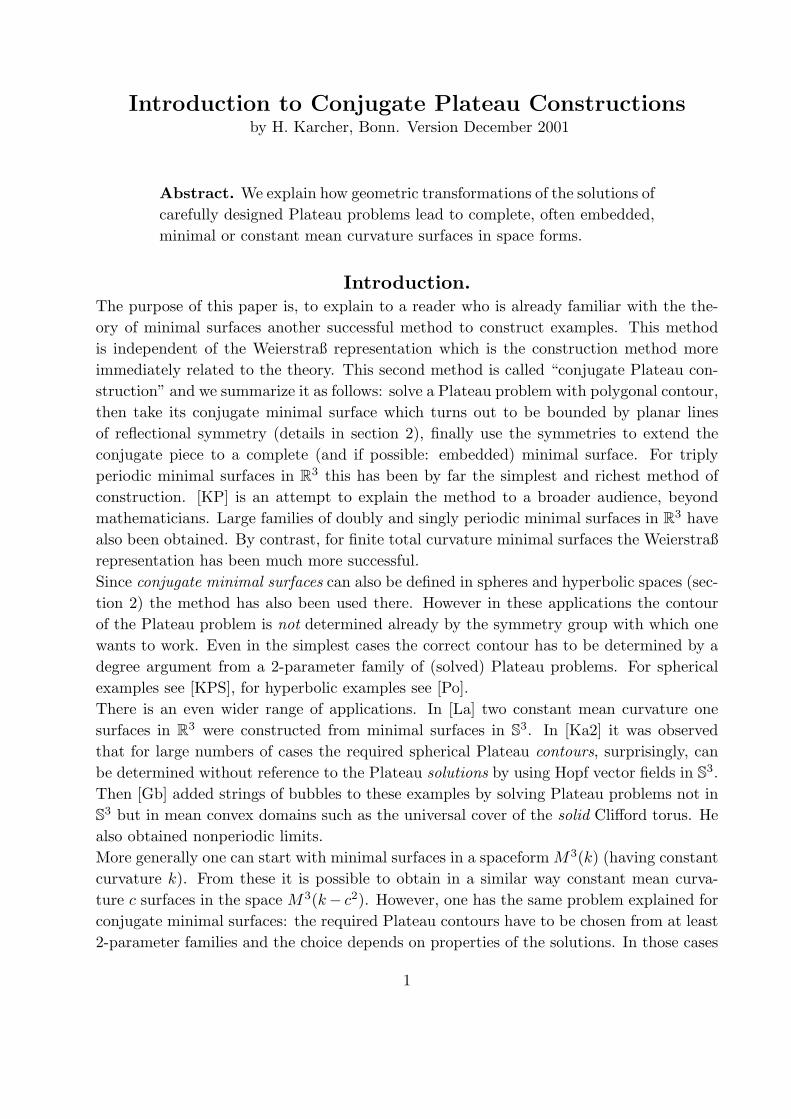
1. Extension of minimal surfaces across boundary segments.Minimal surfaces in R3. More than 50 years before the general Plateau problemwas solved, solutions for certain polygonal contours where found by B. Riemann and byH.A. Schwarz. Their solutions were given as integrals of multivalued functions. In today’sterminology they used the Weierstraß representation on nontrivial Riemann surfaces. Thefollowing particularly simple examples are due to H.A. Schwarz. Consider the followinghexagonal polygons made of edges of a brick with edge lengths a, b, c.P1 : (0, 0, 0)→ (a, 0, 0)→ (a, b, 0)→ (a, b, c)→ (0, b, c)→ (0, 0, c)→ (0, 0, 0),P2 : (0, 0, 0)→ (a, 0, 0)→ (a, b, 0)→ (a, b, c)→ (a, 0, c)→ (0, 0, c)→ (0, 0, 0).

Left: the polygonal contours P1, P2 on the boundary of a cube (a special brick).Right: the contour P2 with its Plateau solution and an extension by 180◦ rota-tions around boundary edges. It is named Schwarz’ CLP-surface.

In both cases the contour has a 1-1 convex projection (in fact many). The Plateau problemhas therefore a unique solution, which is a graph over the interior of the chosen convexprojection. Moreover, by the maximum principle, every compact minimal surface lies inthe convex hull of its boundary. In particular our Plateau solutions are inside the brickwith edge lengths a, b, c. Imagine a black and white (“checkerboard”) tessellation of R3

by these bricks, and imagine our Plateau solution to be in a black brick. The Schwarzreflection theorem says that 180◦ rotation around any of the boundary edges of the Plateau

3

piece gives an analytic continuation of the initial minimal surface piece. Because of the90◦ angles of the polygons we can repeatedly extend across the edges which leave from onepolygon vertex and thus obtain a smooth extension containing that vertex as an interiorpoint. Notice that all the extensions are inside black bricks, and if the extensions leadus back into the first brick then the whole brick comes back in its original position. Thisshows that the extensions lead to embedded triply periodic minimal surfaces. The firstone was named by A. Schoen Schwarz D-surface and the second Schwarz CLP-surface, see[DHKW] vol I, plate V, (a)-(c). The names given by A. Schoen are well known in thecristallographic literature.The cristallographers Fischer and Koch [??] have listed the cristallographic groups whichcontain enough 180◦ rotations so that from segments of the rotation axes polygons can beformed with the property that the Plateau solutions of these polygons extend to embeddedtriply periodic minimal surfaces. Their work includes examples of fairly complicated suchpolygons.

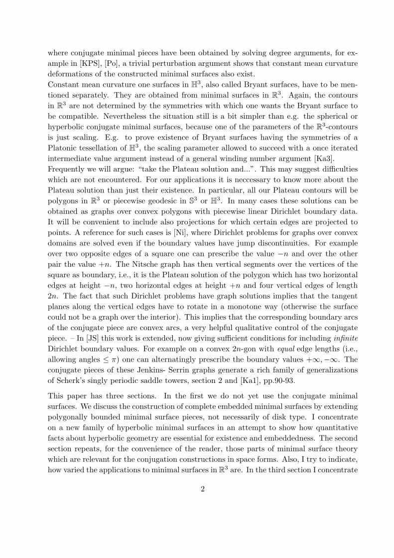
Minimal surfaces in spheres and hyperbolic spaces. Since the Schwarz reflectiontheorem extends to minimal surfaces in spheres and hyperbolic spaces one can extend theabove idea to space forms. Lawson’s minimal surfaces in spheres [La] are constructed inthis way from disk type Plateau solutions bounded by great circle quadrilaterals. I willnow construct new embedded minimal surfaces in hyperbolic space which have compactannular fundamental domains. The purpose of these examples is to illustrate the use ofbarriers and of basic hyperbolic geometry. - Euclidean analogues of such annuli, wherethe annulus is bounded by a pair of equilateral triangles in parallel planes, or a pairof squares in parallel planes, were already constructed by H.A. Schwarz, see [DHKW]vol. I fig. 22 (a),(b),(d) and fig. 23 (a),(b). For more complicated minimal annulisee [Ka2], p.342,343. All these extend to embedded triply periodic minimal surfaces.

Three polygonally bounded minimal annuli in R3, one with noninjective bound-ary. The middle one is called Schwarz’ H-surface.

The existence construction. We have to deal with the following problem: if two cir-cles in parallel planes are too far apart, then there is no catenoid annulus which joinsthem. The problem is dealt with by barriers. In R3 for example, assume that two con-vex polygons in parallel planes are so close together that a catenoid exists which meets

4

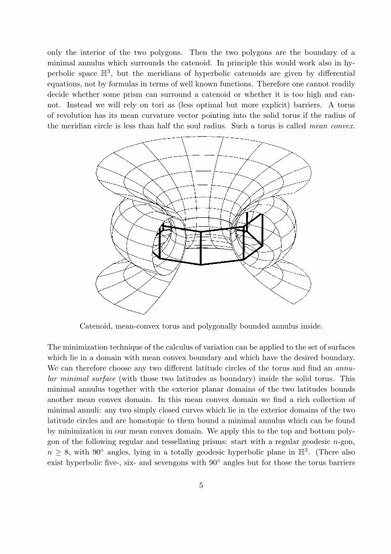
only the interior of the two polygons. Then the two polygons are the boundary of aminimal annulus which surrounds the catenoid. In principle this would work also in hy-perbolic space H3, but the meridians of hyperbolic catenoids are given by differentialequations, not by formulas in terms of well known functions. Therefore one cannot readilydecide whether some prism can surround a catenoid or whether it is too high and can-not. Instead we will rely on tori as (less optimal but more explicit) barriers. A torusof revolution has its mean curvature vector pointing into the solid torus if the radius ofthe meridian circle is less than half the soul radius. Such a torus is called mean convex.

Catenoid, mean-convex torus and polygonally bounded annulus inside.

The minimization technique of the calculus of variation can be applied to the set of surfaceswhich lie in a domain with mean convex boundary and which have the desired boundary.We can therefore choose any two different latitude circles of the torus and find an annu-lar minimal surface (with those two latitudes as boundary) inside the solid torus. Thisminimal annulus together with the exterior planar domains of the two latitudes boundsanother mean convex domain. In this mean convex domain we find a rich collection ofminimal annuli: any two simply closed curves which lie in the exterior domains of the twolatitude circles and are homotopic to them bound a minimal annulus which can be foundby minimization in our mean convex domain. We apply this to the top and bottom poly-gon of the following regular and tessellating prisms: start with a regular geodesic n-gon,n ≥ 8, with 90◦ angles, lying in a totally geodesic hyperbolic plane in H3. (There alsoexist hyperbolic five-, six- and sevengons with 90◦ angles but for those the torus barriers

5

do not work.) Consider next the infinite prism orthogonal to the n-gon in H3. Cut thisinfinite prism above and below its symmetry plane so that the dihedral angles along thetop and bottom rim are 60◦. The following hyperbolic computation shows that the tworims of this prism lie in a mean convex torus (see the figure above) and can therefore bejoined by a minimal annulus (of course inside the convex prism). And analytic extensionof this annulus by repeated 180◦ rotations around boundary edges produces a completeminimal surface which turns out to be embedded.My reference for hyperbolic trigonometry is [Bu, pp.31-42]. It is helpful to know that gen-eral trigonometric formulae simplify more than one expects from the general expressions ifone specializes to simple figures. To emphasize this I only quote and use two such specialcases. First, for right angled triangles with edge lengths a, b, c and angles α, β, γ = π/2 wehave

cosh c = cosh a cosh b = cotα cotβ

sinh a = sinα sinh c = cotβ tanh b

cosα = cosh a sinβ = tanh b coth c.

The formulas cosα = cosh a sinβ, cosh c = cotα cotβ imply that a regular n-gon with 90◦

angles has inradius a = ri and outer radius c = ro given by

cosh ri =cos(π/4)sin(π/n)

, cosh ro = cot(π/4) cot(π/n).

Our second such simple figure is the trirectangle, a quadrilateral with three angles π/2,with edge lengths a, b, α, β and with the fourth angle φ between edges α, β. Here thegeneral formulas simplify to

cosφ = sinh a sinh b = tanhα tanhβ

cosh a = coshα sinφ = tanhβ coth b

sinhα = sinh a coshβ = coth b cotφ.

Next consider the prism over the above 90◦-n-gon, which has at its top rim a dihedral angleof φ = π/3. We determine its inner height hi, i.e., the distance between the top and bottomplane, and its outer height ho, i.e., the distance between the bottom n-gon and the top n-gon (i.e. the distance between the midpoints of the top and bottom edge of a vertical face).Note that a plane through the (vertical) symmetry axis and the midpoint of a (horizontal)edge intersects the prism in a trirectangle with a = hi, b = ri, α = ho, φ = π/3. Withthe formulas cosφ = sinh a sinh b, sinhα = coth b cotφ we get

sinhhi =cos(π/3)sinh ri

, sinhho =cot(π/3)tanh ri

.

Finally we have to check that the two 60◦ rims of the double prism lie in a mean convexdomain as above. For this we choose the midpoint M of the meridian circle of the torus

6

on the extension of the edge ri of the trirectangle and at a distance rs = 1.1 · ri (thesoul radius) from the symmetry axis. The meridian radius rm is determined by cosh rm =coshho cosh(0.1ri) The condition for mean convexity of the torus was rs ≥ 2rm and this issatisfied for n ≥ 8. Therefore we have the existence of a minimal annulus which is boundedby the top and bottom rim of our convex and tessellating hyperbolic prism. For fivegonsto sevengons either this barrier computation is not good enough or the top and bottomrims are indeed too far apart for the minimal annulus to exist. Note another quantitativeaspect of this computation: we do not have other families of such prisms, because the sumof the three dihedral angles at a top vertex of the prism has to be > π; if the sum of thedihedral angles is = π then the vertices of the prism are on the sphere at infinity and if thesum of the dihedral angles is < π then then the vertical edges do not meet the top face.

Analytic extension of the annular piece by 180◦ rotations. By repeated 180◦

rotation around boundary edges the annular fundamental piece is analytically extended toa complete minimal surface. The embeddedness proof has two parts: (i) the constructedannulus is embedded and (ii) the continuation does not create selfintersections. We omitthe first part because the arguments are disjoint from the topic of this paper. For part (ii)we have to understand the tessellation of hyperbolic space by our prisms; such geometricdiscussions are always part of a construction of a complete surface from Plateau pieces.The idea is to color the prisms of the tessellation in red, green and blue so that the colorchanges across a face and 180◦ rotation around an edge of a prism maps that pisma to oneof the same color. If that can be achieved then we have the complete surface containedonly in the prisms of one color. Since along each edge only two prisms of the same colormeet we have avoided selfintersections. We start by making the first prism red, the 2neighbours above and below we make green and the n neighbours across vertical faces wemake blue. Next we describe how the 24 prisms meet which have one vertex in common.Consider how a small sphere around that vertex meets the adjacent prisms: each prismintersects the sphere in a geodesic triangle whose angles are the dihedral angles at thethree edges of the prism at that vertex, i.e., the angles are π/2, π/3, π/3. Four suchtriangles around the π/2-corner fit together to a spherical square with angles 2π/3. Sixsuch squares tessellate the sphere; it is the same tessellation obtained by central projectionof a cube to its circumsphere. The colors of the prisms which meet at one vertex are bydefinition the same as the colors of the 24 triangles of the spherical tessellation and viceversa. Initially we colored four prisms at each vertex of the first prism. Now consider thespherical triangulation which describes the neigbourhood of one vertex of the prism; onecan view it on a cube after subdividing each face by its diagonals into four triangles. Ourcoloring prescription says that opposite triangles on one face have the same colour, sincethey correspond to two prisms whose position differs by a 180◦ rotation about a 90◦ edge.Also, each triangle has neighbours of both other colors. These two observations imply thatthe different colours of two neighbouring triangles determine the colours of all the othertriangles on the cube uniquely. Therefore we can extend the coloration to all the prisms

7

which meet a vertex of the first prism. We continue the coloration and because of theunique extension of a partial coloration to the full sphere we can assign a unique color toeach prism and thus complete the proof.

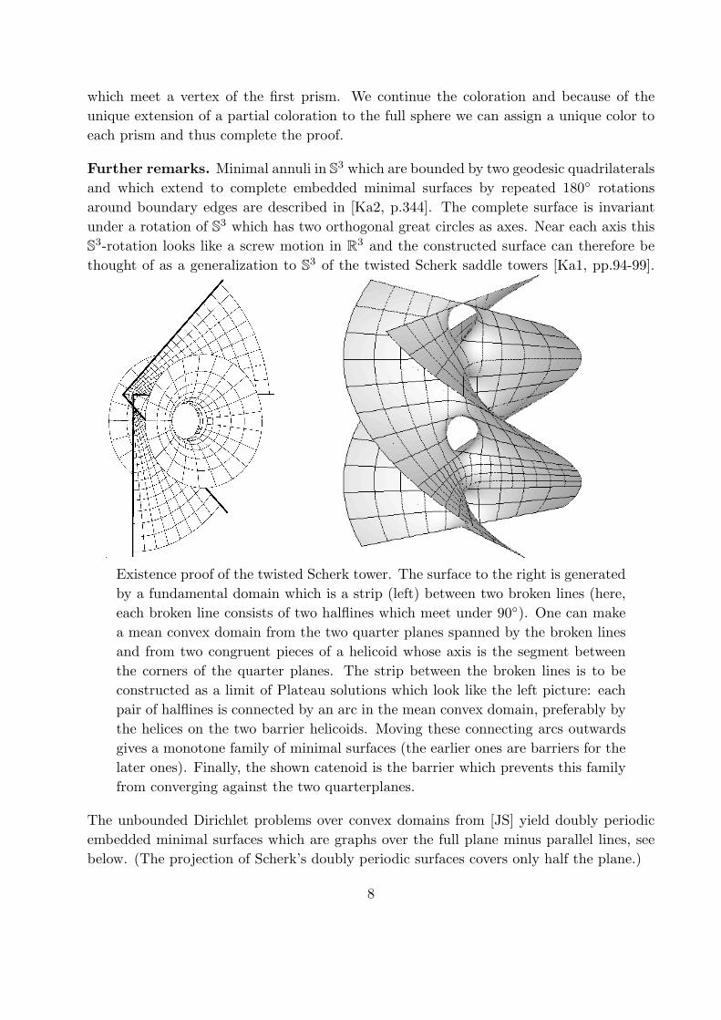
Further remarks. Minimal annuli in S3 which are bounded by two geodesic quadrilateralsand which extend to complete embedded minimal surfaces by repeated 180◦ rotationsaround boundary edges are described in [Ka2, p.344]. The complete surface is invariantunder a rotation of S3 which has two orthogonal great circles as axes. Near each axis thisS3-rotation looks like a screw motion in R3 and the constructed surface can therefore bethought of as a generalization to S3 of the twisted Scherk saddle towers [Ka1, pp.94-99].

Existence proof of the twisted Scherk tower. The surface to the right is generatedby a fundamental domain which is a strip (left) between two broken lines (here,each broken line consists of two halflines which meet under 90◦). One can makea mean convex domain from the two quarter planes spanned by the broken linesand from two congruent pieces of a helicoid whose axis is the segment betweenthe corners of the quarter planes. The strip between the broken lines is to beconstructed as a limit of Plateau solutions which look like the left picture: eachpair of halflines is connected by an arc in the mean convex domain, preferably bythe helices on the two barrier helicoids. Moving these connecting arcs outwardsgives a monotone family of minimal surfaces (the earlier ones are barriers for thelater ones). Finally, the shown catenoid is the barrier which prevents this familyfrom converging against the two quarterplanes.

The unbounded Dirichlet problems over convex domains from [JS] yield doubly periodicembedded minimal surfaces which are graphs over the full plane minus parallel lines, seebelow. (The projection of Scherk’s doubly periodic surfaces covers only half the plane.)

8

A list of the known disk type Plateau solutions for polygonal boundaries, which extend toembedded minimal surfaces, is rather short. However, we see in the next section that theproperties of conjugate minimal surfaces offer very flexible possibilities for the constructionof embedded minimal surfaces. We emphasize that the conjugate surface method of thenext section requires disk type minimal surfaces; the construction of embedded minimalsurfaces from annular (or still higher genus) fundamental domains, which we have seen inthis first section, is not compatible with the definition of the conjugate surface.

2. Conjugate minimal surfaces.Some basic theory. When the theory of minimal surfaces developed in the 19th centuryit was realized early that the three coordinate functions of a conformal parametrizationof a minimal surface are the real parts of holomorphic functions! Since the existence ofconformal parametrizations of surfaces in R3 is a hard theorem which is rarely completelyexplained in differential geometry courses we observe that the above discovery can also bestated without a conformal parametrization. If one imagines an atlas of conformal coor-dinates for the surface, then it makes sense to multiply a tangent vector by the complexnumber i. But this multiplication by i is, on each tangent space, the positive 90◦ rotation,and this is a geometric description of the multiplication by i which does not use a conformalparametrization. The endomorphism field of tangent space wise 90◦ rotations is thereforealso called the complex structure and is denoted by J . A differentiable map from the sur-face to the complex numbers, f : M2 → C is then holomorphic if its differential Tf satisfiesTf(J ·X) = i ·Tf(X) for each tangent vector X. We write f in terms of its real and imagi-nary part, f = u+i·v. Holomorphicity of f then can be expressed as Tu(J ·X) = −Tv(X),or Tv(J ·X) = Tu(X). These Cauchy-Riemann equations say that the differential of theimaginary part can be computed from the differential of the real part and J , namelyTv = −Tu ◦ J . Moreover, just as in C, a differentiable function u is (locally) the real partof a holomorphic function iff the differential form ω := −Tu◦J is closed. Therefore we cannow formulate, without reference to a conformal parametrization, the mentioned discoveryof the 19th century, namely that the coordinate functions of minimal surfaces are, locally,real parts of holomorphic functions. To see why this fact is true requires the use of thesurface equations. Let F : M2 → R3 be a local immersion, N : M2 → S2 the normalGauß map, S the shape operator, g(X,Y ) = 〈TF (X), TF (Y )〉R3 the Riemannian metric,Γ the Christoffel map (or symbol), i.e., T 2F (X,Y )tang = TF ◦ Γ(X,Y ), ∇ the covariantderivative of the metric g and K its curvature, then we have the

Surface equations for TF,N with data {g, S}

TN = TF ◦ S,Weingarten equation

T 2F (X,Y ) = TF ◦ Γ(X,Y ) − g(S ·X,Y )N,Gauß equation

∇2F (X,Y ) := T 2F (X,Y )− TF ◦ Γ(X,Y ) = −g(S ·X,Y )N.Covariant version

9

Integrability conditions:

g(S ·X,Y ) = g(S · Y,X),Symmetry

∇XS · Y = ∇Y S ·X,Codazzi equation

det(S) = K.Gauß equation

trace(S) = 0.Minimality condition:

The close connection between minimal surfaces and holomorphic maps. Theminimal and selfadjoint shape operator S has with respect to an orthonormal basis a trace

free and symmetric matrix(a bb −a

). This implies −K = −det(S) = a2 + b2, hence

S2 = −K · id. This proves the conformality of the normal Gauß map since scalar productschange only by the scaling factor −K:

〈TN(X), TN(Y )〉 = 〈TF (S ·X), TF (S · Y )〉 = g(S ·X,S · Y ) = −K · g(X,Y ).

In particular, we obtain the meromorphic Gauß map G if we compose the normal Gaußmap N (which is orientation reversing but angle preserving) with an orientation reversing(and angle preserving) stereographic projection St : S2 → C as follows G := St ◦N .

The complex structure J has with respect to any orthonormal basis the matrix(

0 −11 0

).

This and the above matrix of S (which was implied by minimality and symmetry) give

J ◦ S =(−b aa b

)= −S ◦ J . This implies first that S∗ := J ◦ S is again symmetric and

has trace(S∗) = 0. Secondly, det(J) = 1 implies that the Gauß equations for S and S∗ areequivalent. And finally ∇J = 0, i.e. ∇S∗ = J ·∇S, implies that the Codazzi equations forS and S∗ are also equivalent. Therefore g, S∗ satisfy the integrability conditions and defineanother minimal immersion F ∗ (of simply connected pieces or coverings). These two pairsof surface data, {g, S} and {g, S∗}, belong to minimal immersions F, F ∗ which fit togetheras real and imaginary part of a holomorphic map F + i · F ∗ for the following reason. Werewrote the second surface equation in its covariant form. This shows immediately thatthe covariant derivative of the (R3-valued) 1-form TF , which is equal to −g(S ·X,Y )N ,has trace 0 so that the three coordinate functions F j are Riemannian harmonic. Togetherwith ∇J = 0 the covariant surface equation shows further that the derivative of the (R3-valued) 1-form TF · J , which is equal to −g(S · J · X,Y )N , is again symmetric (equalto −g(X,S · J · Y )N), i.e. the exterior derivative of TF ◦ J is 0. Therefore TF ◦ Jis (on simply connected domains again) the derivative of some other map. If we defineF ∗ by TF ∗ := −TF ◦ J then we have proved that the surface equations for {TF,N}with data {g, S} imply immediately that {TF ∗, N∗ := N} are solutions for the surfaceequations with data {g, S∗}. F ∗ is called the conjugate minimal immersion. Moreover,

10

F + iF ∗ : M2 → C3 is not only differentiable but even holomorphic because the Cauchy-Riemann equations T (F+iF ∗)·J = i·T (F+iF ∗) are satisfied. For numerical computationsit has been extremely convenient that F ∗ can be obtained by one integration from firstderivative data, namely from TF ∗ := −TF ◦ J . (The second order surface data {g, J ◦S},which are numerically more difficult to obtain, determine the surface via an ODE.)

Extension of “conjugate minimal surfaces” to S3 and H3. Some of these obser-vations carry over to minimal surfaces in spheres S3(c2) or hyperbolic spaces H3(−c2) ofcurvature c2 resp. −c2. One cannot speak of harmonic coordinate functions of minimalsurfaces in these spaces. But the surface equations and the integrability conditions arealmost the same. One only has to interprete N as a unit normal field along the immersionF , then the surface equations hold. The first two integrability conditions stay the sameand the Gauß equation needs only a small adjustment:

k + det(S) = K.Gauß equation in M3(k):

Therefore: if {g, S} are minimal surface data in a space M3(k) of constant curvature k,then {g, (id cosα + J sinα) · S} is a 1-parameter family of isometric (and in general non-congruent) minimal surface data in M3(k), the socalled associate family.

Extension to constant mean curvature surfaces. In fact, minimal surface data {g, S}in one space form M(k) provide constant mean curvature ±c surface data {g, S± c · id} inanother space form M(k − c2). I learnt this from [La], I am told Lawson heard this fromCalabi and in any case, it is immediate from the surface equations and their integrabilityconditions since det(S ± c · id) = det(S) + c2. We will use this in section 3.

Symmetry lines of minimal surfaces. Before we can exploit this geometric trans-formation of a simply connected minimal surface to its conjugate minimal surface weneed one more piece of geometric information. The usual Frenet theory of curves in 3-dimensional space forms fails at points where the curve has curvature = 0; in particularit cannot handle geodesics. This problem goes away for curves on surfaces. Given a unitspeed curve γ in the domain of a parametrized surface F : D2 → M3 with normal fieldN : D2 → TM3, N(p) ⊥ image(TFp). We then choose as frame along the image curvec := F ◦ γ the tangent field e1 := TF (γ), the conormal field e2 := TF (J · γ), and the sur-face normal field e3 := N ◦ γ. We then have with geodesic curvature κg, normal curvaturekn = 〈e3, e1〉 = g(Sγ, γ) and normal torsion τn = 〈e3, e2〉 = g(Sγ, J · γ) the following

Frenet equations for curves on surfaces:

e1 = κg · e2 − kn · e3, e2 = −κg · e1 − τn · e3, e3 = kn · e1 + τn · e2.

κ∗g = κg, k∗n = −τn, τ∗n = kn.Data on the conjugate surface:

We discuss these equations for geodesics, i.e. κg = 0. Curves are principal curvature linesiff τn = 0 and asymptote lines (vanishing normal curvature) iff kn = 0. Observe that a

11

principal curvature line on a minimal immersion is an asymptote line on the conjugateimmersion and vice versa. But a geodesic asymptote line has vanishing tangential andnormal curvature, hence is even a geodesic in the space form M(k). Consider next ageodesic curvature line; the Frenet equations show (i) that the surface normal N ◦ γ is theprincipal curvature normal of the curve and (ii) that its torsion in M(k) is 0, i.e., such acurve is planar (or lies in a 2-dimensional totally geodesic subspace). Finally, for minimalsurfaces in any space form we have the

Reflection principle for minimal surfaces in M3(k):a) 180◦ rotation around a geodesic asymptote line (in fact a geodesic in M3(k)) is acongruence of the minimal surface.b) Reflection in the plane of a geodesic principle curvature line is a congruence of theminimal surface.c) Plateau solutions in polygonal contours are sufficiently regular at the boundary so that thesymmetry from a) can be used to analytically extend the Plateau piece across each boundarysegment. If the conjugate surface is considered then this extension is transformed into thesymmetry b).

Embeddedness criterion. The integration of the surface equations usually does not saywhether the obtained immersion is in fact an embedding. The following result is an easilyapplied criterion which covers many interesting cases.R. Krust’s conjugate graph theorem in R3:If a minimal surface is a graph over a convex domain then all surfaces of the associatefamily are graphs (usually not over convex domains) and hence embedded, [DHKW], 118-119.

Some singly periodic examples in R3. (I give more details for the triply periodiccase.) The conjugates of Jenkins-Serrin graphs over equilateral convex 2n-gons were alreadyquoted in the introduction. Being equilateral is a trivial sufficient condition under whichthe results of [JS] can be applied. And the fact that the strips between the vertical linesof the graph all have the same width implies that, on the conjugate graph, all the pairs ofhorizontal symmetry lines have the same vertical distance. These conjugate patches arefundamental domains for a rich family of deformations of the singly periodic Scherk saddletowers. Embeddedness follows from Krust’s theorem. — Each pair of adjacent saddles ofthe most symmetric of these saddle towers were connected by a “catenoid like” handle in[Ka1], p. 107-110, giving toroidal saddle towers.The Jenkins-Serrin criterion allows certain angles of the convex polygon to be equal to π.Corresponding neighboring wings of the saddle tower are then parallel. This suggests to“cut one pair of such parallel wings off, modify the cuts to be planar symmetry lines andreflect to get other toroidal saddle towers”. Technically this is done by replacing the bound-ary values ±∞ of the pair of edges with angle π between them by finite boundary values±n. The boundary symmetry lines corresponding to the two horizontal edges at height ±n

12

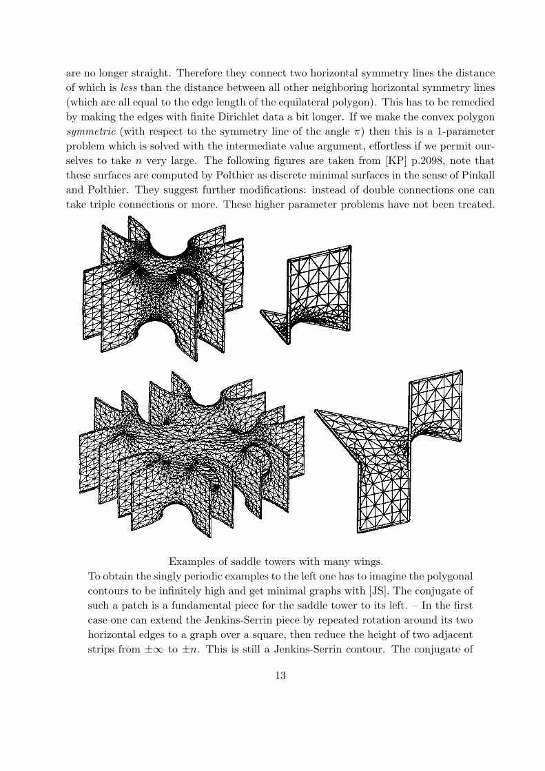
are no longer straight. Therefore they connect two horizontal symmetry lines the distanceof which is less than the distance between all other neighboring horizontal symmetry lines(which are all equal to the edge length of the equilateral polygon). This has to be remediedby making the edges with finite Dirichlet data a bit longer. If we make the convex polygonsymmetric (with respect to the symmetry line of the angle π) then this is a 1-parameterproblem which is solved with the intermediate value argument, effortless if we permit our-selves to take n very large. The following figures are taken from [KP] p.2098, note thatthese surfaces are computed by Polthier as discrete minimal surfaces in the sense of Pinkalland Polthier. They suggest further modifications: instead of double connections one cantake triple connections or more. These higher parameter problems have not been treated.

Examples of saddle towers with many wings.To obtain the singly periodic examples to the left one has to imagine the polygonalcontours to be infinitely high and get minimal graphs with [JS]. The conjugate ofsuch a patch is a fundamental piece for the saddle tower to its left. – In the firstcase one can extend the Jenkins-Serrin piece by repeated rotation around its twohorizontal edges to a graph over a square, then reduce the height of two adjacentstrips from ±∞ to ±n. This is still a Jenkins-Serrin contour. The conjugate of

13

its minimal graph generates a saddle tower where one pair of wings has finitelength. Two such surfaces fit together along the pair of symmetry lines betweenthem after one adjusts one parameter, see text above.

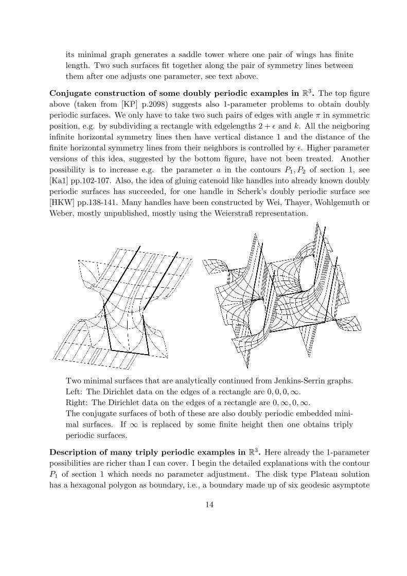
Conjugate construction of some doubly periodic examples in R3. The top figureabove (taken from [KP] p.2098) suggests also 1-parameter problems to obtain doublyperiodic surfaces. We only have to take two such pairs of edges with angle π in symmetricposition, e.g. by subdividing a rectangle with edgelengths 2 + ε and k. All the neigboringinfinite horizontal symmetry lines then have vertical distance 1 and the distance of thefinite horizontal symmetry lines from their neighbors is controlled by ε. Higher parameterversions of this idea, suggested by the bottom figure, have not been treated. Anotherpossibility is to increase e.g. the parameter a in the contours P1, P2 of section 1, see[Ka1] pp.102-107. Also, the idea of gluing catenoid like handles into already known doublyperiodic surfaces has succeeded, for one handle in Scherk’s doubly periodic surface see[HKW] pp.138-141. Many handles have been constructed by Wei, Thayer, Wohlgemuth orWeber, mostly unpublished, mostly using the Weierstraß representation.

Two minimal surfaces that are analytically continued from Jenkins-Serrin graphs.Left: The Dirichlet data on the edges of a rectangle are 0, 0, 0,∞.Right: The Dirichlet data on the edges of a rectangle are 0,∞, 0,∞.The conjugate surfaces of both of these are also doubly periodic embedded mini-mal surfaces. If ∞ is replaced by some finite height then one obtains triplyperiodic surfaces.

Description of many triply periodic examples in R3. Here already the 1-parameterpossibilities are richer than I can cover. I begin the detailed explanations with the contourP1 of section 1 which needs no parameter adjustment. The disk type Plateau solutionhas a hexagonal polygon as boundary, i.e., a boundary made up of six geodesic asymptote

14

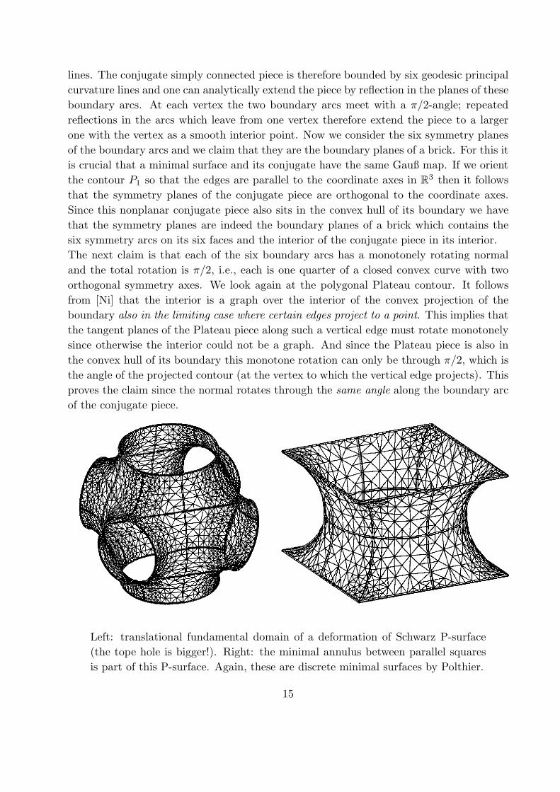
lines. The conjugate simply connected piece is therefore bounded by six geodesic principalcurvature lines and one can analytically extend the piece by reflection in the planes of theseboundary arcs. At each vertex the two boundary arcs meet with a π/2-angle; repeatedreflections in the arcs which leave from one vertex therefore extend the piece to a largerone with the vertex as a smooth interior point. Now we consider the six symmetry planesof the boundary arcs and we claim that they are the boundary planes of a brick. For this itis crucial that a minimal surface and its conjugate have the same Gauß map. If we orientthe contour P1 so that the edges are parallel to the coordinate axes in R3 then it followsthat the symmetry planes of the conjugate piece are orthogonal to the coordinate axes.Since this nonplanar conjugate piece also sits in the convex hull of its boundary we havethat the symmetry planes are indeed the boundary planes of a brick which contains thesix symmetry arcs on its six faces and the interior of the conjugate piece in its interior.The next claim is that each of the six boundary arcs has a monotonely rotating normaland the total rotation is π/2, i.e., each is one quarter of a closed convex curve with twoorthogonal symmetry axes. We look again at the polygonal Plateau contour. It followsfrom [Ni] that the interior is a graph over the interior of the convex projection of theboundary also in the limiting case where certain edges project to a point. This implies thatthe tangent planes of the Plateau piece along such a vertical edge must rotate monotonelysince otherwise the interior could not be a graph. And since the Plateau piece is also inthe convex hull of its boundary this monotone rotation can only be through π/2, which isthe angle of the projected contour (at the vertex to which the vertical edge projects). Thisproves the claim since the normal rotates through the same angle along the boundary arcof the conjugate piece.

Left: translational fundamental domain of a deformation of Schwarz P-surface(the tope hole is bigger!). Right: the minimal annulus between parallel squaresis part of this P-surface. Again, these are discrete minimal surfaces by Polthier.

15

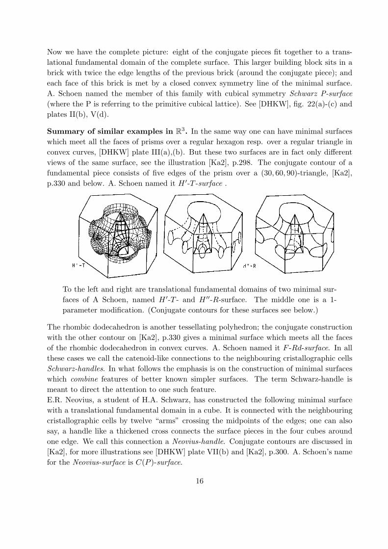
Now we have the complete picture: eight of the conjugate pieces fit together to a trans-lational fundamental domain of the complete surface. This larger building block sits in abrick with twice the edge lengths of the previous brick (around the conjugate piece); andeach face of this brick is met by a closed convex symmetry line of the minimal surface.A. Schoen named the member of this family with cubical symmetry Schwarz P-surface(where the P is referring to the primitive cubical lattice). See [DHKW], fig. 22(a)-(c) andplates II(b), V(d).

Summary of similar examples in R3. In the same way one can have minimal surfaceswhich meet all the faces of prisms over a regular hexagon resp. over a regular triangle inconvex curves, [DHKW] plate III(a),(b). But these two surfaces are in fact only differentviews of the same surface, see the illustration [Ka2], p.298. The conjugate contour of afundamental piece consists of five edges of the prism over a (30, 60, 90)-triangle, [Ka2],p.330 and below. A. Schoen named it H ′-T -surface .

To the left and right are translational fundamental domains of two minimal sur-faces of A Schoen, named H ′-T - and H ′′-R-surface. The middle one is a 1-parameter modification. (Conjugate contours for these surfaces see below.)

The rhombic dodecahedron is another tessellating polyhedron; the conjugate constructionwith the other contour on [Ka2], p.330 gives a minimal surface which meets all the facesof the rhombic dodecahedron in convex curves. A. Schoen named it F -Rd-surface. In allthese cases we call the catenoid-like connections to the neighbouring cristallographic cellsSchwarz-handles. In what follows the emphasis is on the construction of minimal surfaceswhich combine features of better known simpler surfaces. The term Schwarz-handle ismeant to direct the attention to one such feature.E.R. Neovius, a student of H.A. Schwarz, has constructed the following minimal surfacewith a translational fundamental domain in a cube. It is connected with the neighbouringcristallographic cells by twelve “arms” crossing the midpoints of the edges; one can alsosay, a handle like a thickened cross connects the surface pieces in the four cubes aroundone edge. We call this connection a Neovius-handle. Conjugate contours are discussed in[Ka2], for more illustrations see [DHKW] plate VII(b) and [Ka2], p.300. A. Schoen’s namefor the Neovius-surface is C(P )-surface.

16

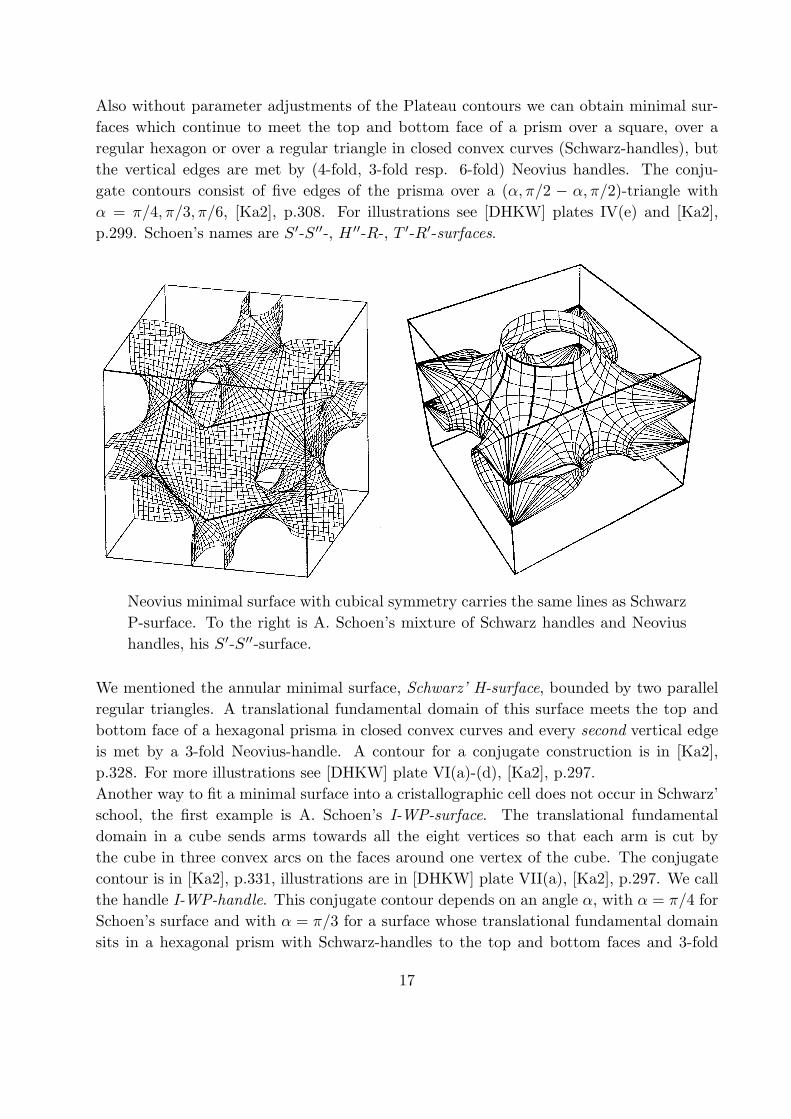
Also without parameter adjustments of the Plateau contours we can obtain minimal sur-faces which continue to meet the top and bottom face of a prism over a square, over aregular hexagon or over a regular triangle in closed convex curves (Schwarz-handles), butthe vertical edges are met by (4-fold, 3-fold resp. 6-fold) Neovius handles. The conju-gate contours consist of five edges of the prisma over a (α, π/2 − α, π/2)-triangle withα = π/4, π/3, π/6, [Ka2], p.308. For illustrations see [DHKW] plates IV(e) and [Ka2],p.299. Schoen’s names are S′-S′′-, H ′′-R-, T ′-R′-surfaces.

Neovius minimal surface with cubical symmetry carries the same lines as SchwarzP-surface. To the right is A. Schoen’s mixture of Schwarz handles and Neoviushandles, his S′-S′′-surface.

We mentioned the annular minimal surface, Schwarz’ H-surface, bounded by two parallelregular triangles. A translational fundamental domain of this surface meets the top andbottom face of a hexagonal prisma in closed convex curves and every second vertical edgeis met by a 3-fold Neovius-handle. A contour for a conjugate construction is in [Ka2],p.328. For more illustrations see [DHKW] plate VI(a)-(d), [Ka2], p.297.Another way to fit a minimal surface into a cristallographic cell does not occur in Schwarz’school, the first example is A. Schoen’s I-WP-surface. The translational fundamentaldomain in a cube sends arms towards all the eight vertices so that each arm is cut bythe cube in three convex arcs on the faces around one vertex of the cube. The conjugatecontour is in [Ka2], p.331, illustrations are in [DHKW] plate VII(a), [Ka2], p.297. We callthe handle I-WP-handle. This conjugate contour depends on an angle α, with α = π/4 forSchoen’s surface and with α = π/3 for a surface whose translational fundamental domainsits in a hexagonal prism with Schwarz-handles to the top and bottom faces and 3-fold

17

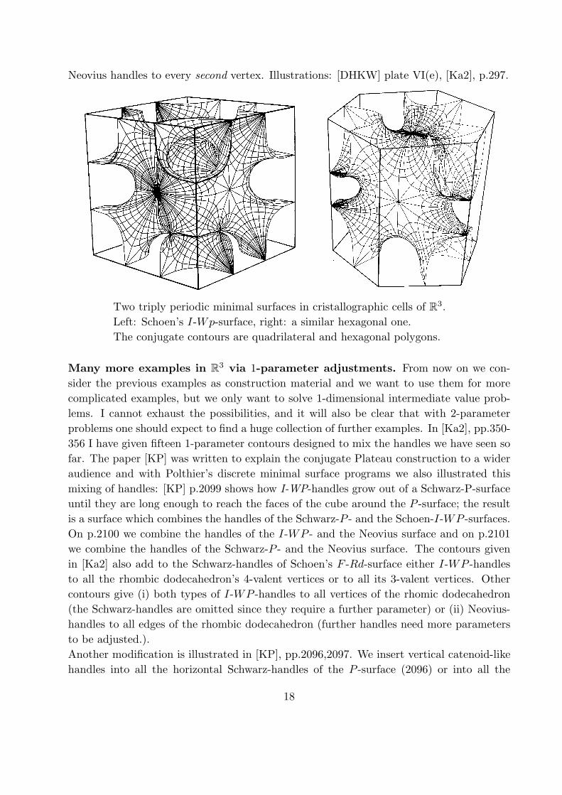
Neovius handles to every second vertex. Illustrations: [DHKW] plate VI(e), [Ka2], p.297.

Two triply periodic minimal surfaces in cristallographic cells of R3.Left: Schoen’s I-Wp-surface, right: a similar hexagonal one.The conjugate contours are quadrilateral and hexagonal polygons.

Many more examples in R3 via 1-parameter adjustments. From now on we con-sider the previous examples as construction material and we want to use them for morecomplicated examples, but we only want to solve 1-dimensional intermediate value prob-lems. I cannot exhaust the possibilities, and it will also be clear that with 2-parameterproblems one should expect to find a huge collection of further examples. In [Ka2], pp.350-356 I have given fifteen 1-parameter contours designed to mix the handles we have seen sofar. The paper [KP] was written to explain the conjugate Plateau construction to a wideraudience and with Polthier’s discrete minimal surface programs we also illustrated thismixing of handles: [KP] p.2099 shows how I-WP-handles grow out of a Schwarz-P-surfaceuntil they are long enough to reach the faces of the cube around the P -surface; the resultis a surface which combines the handles of the Schwarz-P - and the Schoen-I-WP -surfaces.On p.2100 we combine the handles of the I-WP - and the Neovius surface and on p.2101we combine the handles of the Schwarz-P - and the Neovius surface. The contours givenin [Ka2] also add to the Schwarz-handles of Schoen’s F -Rd-surface either I-WP -handlesto all the rhombic dodecahedron’s 4-valent vertices or to all its 3-valent vertices. Othercontours give (i) both types of I-WP -handles to all vertices of the rhomic dodecahedron(the Schwarz-handles are omitted since they require a further parameter) or (ii) Neovius-handles to all edges of the rhombic dodecahedron (further handles need more parametersto be adjusted.).Another modification is illustrated in [KP], pp.2096,2097. We insert vertical catenoid-likehandles into all the horizontal Schwarz-handles of the P -surface (2096) or into all the

18

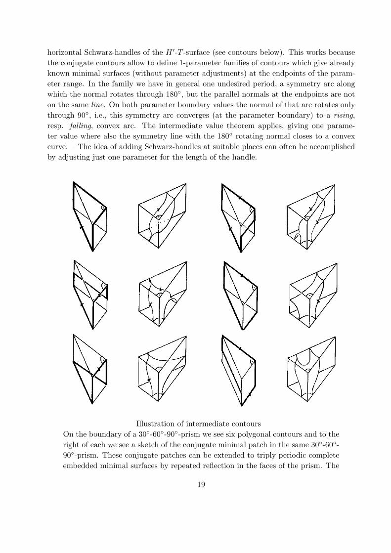
horizontal Schwarz-handles of the H ′-T -surface (see contours below). This works becausethe conjugate contours allow to define 1-parameter families of contours which give alreadyknown minimal surfaces (without parameter adjustments) at the endpoints of the param-eter range. In the family we have in general one undesired period, a symmetry arc alongwhich the normal rotates through 180◦, but the parallel normals at the endpoints are noton the same line. On both parameter boundary values the normal of that arc rotates onlythrough 90◦, i.e., this symmetry arc converges (at the parameter boundary) to a rising,resp. falling, convex arc. The intermediate value theorem applies, giving one parame-ter value where also the symmetry line with the 180◦ rotating normal closes to a convexcurve. – The idea of adding Schwarz-handles at suitable places can often be accomplishedby adjusting just one parameter for the length of the handle.

Illustration of intermediate contoursOn the boundary of a 30◦-60◦-90◦-prism we see six polygonal contours and to theright of each we see a sketch of the conjugate minimal patch in the same 30◦-60◦-90◦-prism. These conjugate patches can be extended to triply periodic completeembedded minimal surfaces by repeated reflection in the faces of the prism. The

19

three pentagonal contours lead to surfaces of A.Schoen without period killing.The three hexagons have one horizontal edge on a face of the prism and one hasto use the intermediate value theorem to find the correct height of this edge. Thecontour to the right in the first row gives the surface between Schoen’s H ′-T - andH ′′-R-surfaces above. The other two intermediate contours add vertical handlestowards the horizontal faces of the hexagonal prism.

One can also insert a 4-fold Neovius-handle into the vertical necks of the Schwarz-P -surface.This splits each vertical catenoid like neck into four thinner parallel ones, [KP], p.2104.Analogous modifications apply to other surfaces of the “construction material”.In all the highly symmetric cristallographic prisms we have seen surfaces with verticalSchwarz handles but with different types of horizontal handles (Schwarz- and Neovius-handles). In the quadratic prism we have Schwarz’ P -surface and Schoen’s S-S′-surface;in the hexagonal prism we have Schoen’s H ′-T - and H ′′-R- and Schwarz’ H-surfaces andsimilar examples exist in the prisms over equilateral triangles.

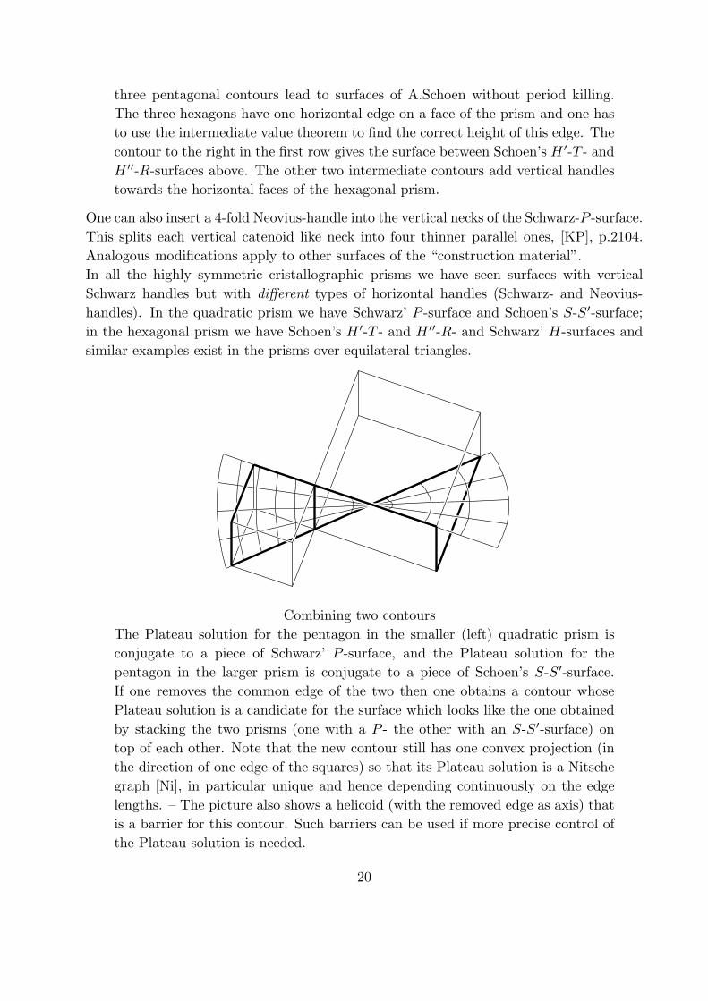
Combining two contoursThe Plateau solution for the pentagon in the smaller (left) quadratic prism isconjugate to a piece of Schwarz’ P -surface, and the Plateau solution for thepentagon in the larger prism is conjugate to a piece of Schoen’s S-S′-surface.If one removes the common edge of the two then one obtains a contour whosePlateau solution is a candidate for the surface which looks like the one obtainedby stacking the two prisms (one with a P - the other with an S-S′-surface) ontop of each other. Note that the new contour still has one convex projection (inthe direction of one edge of the squares) so that its Plateau solution is a Nitschegraph [Ni], in particular unique and hence depending continuously on the edgelengths. – The picture also shows a helicoid (with the removed edge as axis) thatis a barrier for this contour. Such barriers can be used if more precise control ofthe Plateau solution is needed.

20

One observes that the convex symmetry lines on the top and bottom faces of the prismsare almost circles, see also [KP], pp.2096,2097. This suggests to glue one of these ontop of the other, minimally of course. The above figure explains why this is an easytask for the conjugate contour: just put the two contours together along the edge whichcorresponds to the horizontal symmetry line; then omit that edge. One problem remainsto be solved by an 1-parameter adjustment: the two types of horizontal handles must havethe same length, i.e., their vertical symmetry planes (which are by constrcution parallel)must coincide. If the common height of the two prisms converges to zero then the Plateausolutions converge to the union of two squares, and so do their conjugate patches. Thissays that those handles, which come from the part of the contour over the smaller square,are the shorter ones, at least for very small heights of the prims. Continuity and theintermediate value theorem finish the proof.I hope this is enough to convince the reader that the conjugate Plateau method for minimalsurfaces in R3 is so flexible that already with contours, where only one parameter has tobe adjusted, we can obtain a very large collection of triply periodic minimal surfaces. Inmost cases embeddedness comes for free because the Plateau contour is a graph, by Krust’stheorem the conjugate piece is embedded and the different congruent pieces sit in differentfundamental cells for the symmetry group in question. – One would also expect that thepossibilities for 2-parameter adjustments are more than one would like to describe.

3. Conjugate constant mean curvature surfaces.Recall from section 2: if we are given minimal surface data {g, S} (Riemannian metric gand Weingarten map S) in a space of constant curvature k, M3(k), then {g, S ± c · id} aresurface data for a constant mean curvature ±c surface in M3(k − c2). Such surface datacan be integrated on simply connected domains. The constant mean curvature surfacehas been called the cousin of the minimal surface. In the examples of section 2 we haveseen that the transition from a polygonally bounded Plateau piece to the conjugate surfacebounded by planar lines of reflectional symmetry is the main reason for the flexibility ofthis method. This is true even more for the transition to constant mean curvature surfacesbecause only the geodesic principle curvature lines allow to use a symmetry of the spaceM3, namely a reflection, to analytically extend the original piece. Then one speaks of aconstant mean curvature conjugate cousin surface if the data {g, S} of the minimal surfaceare changed to {g, J · S ± c · id} (with J the complex structure, the positive 90◦ rotation).Quite remarkably it turns out that the derivative TF ∗ of the cmc1 conjugate cousin in R3

can be obtained explicitly from the derivative TF of the corresponding minimal surfacein S3 and from the complex structure J ; one does not have to relate these through thesecond order surface data. In conjugate cousin constructions one allways assumes that theminimal piece has a geodesic polygon as boundary so that the conjugate cousin is boundedby planar symmetry lines. Of course, the angles between the geodesic edges are the sameas the angles between the planar symmetry arcs at corresponding vertices, and these angleshave to be of the form 2π/k, k ∈ N so that the extended surface (by repeated reflections)

21

has the vertices as smooth interior points.

We first need to understand why the general case is so much more difficult than the caseof conjugate minimal surfaces in R3 in section 2. Then we can appreciate the extra helpwhich we get from the group structure of S3 when we use the conjugate cousin method toconstruct constant mean curvature one surfaces in R3. We have the simplest case possibleif we start with a disk type minimal Plateau solution in a nonplanar geodesic quadrilateralwith angles of the form 2π/k. The conjugate minimal piece and all the conjugate cousinsare then bounded by four planar symmetry arcs. Extension by reflections in the two arcsthat meet at one vertex then gives a larger surface with that vertex as smooth interiorpoint. Moreover, if the quadrilateral was chosen with some care then the four symmetryplanes of the boundary arcs are boundary planes of a simplex in M3 that contains theconjugate cousin piece. This is the situation in [Sm], [KPS], parts of [Po] and also in [Ka3].For the construction of complete embedded minimal or cousin surfaces the difficulty beginsnow:

We need to guarantee that the above simplex (made from the boundary symmetryplanes of the cousin piece) tessellates M3(k − c2).

Note that the cousin piece meets the faces of the simplex orthogonally. This means thatthe dihedral angle between any pair of symmetry planes that meet at one vertex is alsothe angle between the corresonding symmetry lines on the surface and therefore is one ofthe angles of the quadrilateral Plateau contour. In other words, four of the six dihedralangles of the simplex are known as the angles of the quadrilateral. The problem is tocontrol the other two dihedral angles of the simplex. This is much simpler in R3 (wherethe scalar product of the normals of the planes gives the desired dihedral angle) than in acurved space. In the applications of [KPS], [Po] and [Ka3] the simplex is a fundamentaldomain for the symmetry group of a platonic polyhedron. This means that it has threedihedral angles equal to π/2; these and a fourth one are the angles given by the angles ofthe conjugate Plateau quadrilateral, as we said before. The simplification caused by theπ/2-angles is that the remaining two dihedral angles of the simplex are also face angles ofthis simplex. But each such face angle is the angle between the normals at the endpointsof a boundary arc because these normals are edges of the simplex.In R3 such an angle is the same as the total curvature of the symmetry arc and thereforealso the same as the total rotation of the tangent plane of the Plateau piece along the edgeunder consideration.

This means in particular: In R3 this angle is determined by the Plateau contouralone, without reference to the Plateau solution.

In spheres and hyperbolic spaces the Gauß-Bonnet theorem says that the total curvatureand the desired angle between the end point normals differ by the area of the curvedtriangle that is bounded by the symmetry arc and its two endpoint normals. Therefore theremaining dihedral angles are not computable from the Plateau contour alone, but theycan be estimated if one has good bounds for the Plateau solution.

22

A quadrilateral with prescribed angles has two free parameters in spheres, Euclidean andhyperbolic spaces and we have to choose those so that the two remaining dihedral anglesof the simplex around the conjugate cousin have the correct values. One therefore hasto find a closed curve in the 2-dimensional parameter space so that the image curve ofthe pairs of dihedral angles has winding number =/ 0 with respect to the correct pair ofdihedral angles. This argument gets simpler for Bryant surfaces since one of the domainparameters can be specified as a function of the other such that along the correspondingcurve one of the two dihedral angles is always correct while the other is too small at oneend and too large at the other. The completion of these arguments requires so much workthat only the mentioned simplest cases are treated in [KPS], [Po] and [Ka3]. One is farfrom the flexibility which we saw in the applications in section 2 to triply periodic minimalsurfaces in R3.

Conjugate cousins in R3. The preceding discussion directs some extra attention to thecase of constant mean curvature one surfaces in R3, considered as conjugate cousins ofminimal surfaces in S3. In these cases the remaining dihedral angles are now known to becomputable from the spherical Plateau contour without reference to the Plateau solution.But how explicitly can this be done? The answer is very nice. Consider S3 as a group, e.g.as the unit quaternions. The parallel translations of R3 are replaced by the left translationsLq : S3 → S3, Lq(p) := q · p. With these isometries we can extend every tangent vectorX ∈ TidS3 to a left invariant vectorfield X∗ by X∗(q) := TLq|id(X) = q · X. Such aleft invariant vector field has constant length, the angle between two such vector fields isconstant and the integral curves of these vector fields are great circles, e.g. if |X| = 1 thent 7→ cos(t) · q+ sin(t) ·X∗(q) is the integral curve through q. And clearly, each great circleis integral curve of exactly one unit length left invariant vector field. All this is in completeanalogy to parallel vector fields on R3. With these notions the answer is:

Measure the total rotation of the tangent plane of the Plateau piece along a greatcircle edge against left invariant vector fields then this total rotation is the sameas the angle between the normals at the endpoints of the symmetry arc (whichcorresponds to the edge under consideration) of the conjugate cousin surface.

This says in particular that we can explicitly determine the great circle Plateau contours ifwe have decided which angles between symmetry planes we want to achieve. For exampleall the conjugate contours for triply periodic minimal surfaces in R3 which did not requireany parameter adjustment can now be translated into great circle polygons such that theconjugate cousins of their Plateau solutions give immersed constant mean curvature onesurfaces in R3 with the same symmetry groups as the minimal surfaces. A slightly differentpicture is: Scale the conjugate cousins made from very small spherical polygons up to havethe same periods as the minimal surfaces, then we get small constant mean curvaturedeformations of the minimal surfaces. Such small deformations continue to be embedded.Moreover, there are deformations which are not interesting for the minimal surface: If welet the edgelength a of the contour P1 in section 1 shrink to 0 then we get a planar contour

23

and a planar minimal piece. However the corresponding spherical quadrilateral does notlie in a great sphere, therefore we get a nontrivial Plateau piece and the correspondingdoubly periodic constant mean curvature one cousin looks like one horizontal layer of theminimal surface, but with the vertical Schwarz handles between layers having shrunk tozero size.Since we get in this way without effort many triply periodic cmc1 surfaces together withdoubly periodic degenerations, it is clear that with a little effort one can get many morefamilies of cmc1 surfaces. Among the surfaces one obtains that way are triply periodic oneswhich almost look like sphere packings; the large handles of the related minimal surfacehave shrunk to very small catenoid like connections between the spheres. In the work ofN. Kapouleas portions of his surfaces are very close to very long strings of spheres. It istherefore a natural question how close to such examples one can come with the conjugatecousin method. Here a successful idea was to solve “spherical” Plateau problems not reallyin the sphere but for example in the universal cover of the solid Clifford torus [Gb]. Thismodification indeed allows to replace the catenoid like connectors between spheres by longstrings of spheres with tiny necks between them.

Proof of the explicit relation between the differentials of minimal surfaces in S3 and thedifferentials of their cmc1 conjugate cousins in R3. We need three steps. The first treats

Cross product and complex structure. For a 2-dimensional surface M2 with normalfield N in a 3-dimensional space M3 we have a simple relation between the complexstructure J of M2 and the normal N via the cross product in the tangent spaces of M3.Usually the orientations are chosen so that for each tangent vector X of M2 holds

X × JX = N or JX = N ×X.

An immediate application is the fact that J is a covariantly parallel endomorphism field.Recall that a tangent vectorfield t 7→ X(t) to M2 along a curve t 7→ c(t) is called covariantlyparallel along c, iff the covariant derivative ∇dtX(t) in M3 is orthogonal to M2. As in Rn

extend this definition and call an endomorphism field covariantly parallel iff it maps parallelvector fields to parallel vector fields. The endomorphism field J has this property becauseof

∇dt

(JX) =∇dt

(N ×X) =∇dtN ×X +N × ∇

dtX ∼ N + 0 ⊥M2.

This parallelity is important because it says that for the covariant differentiation Ddt of

M2 (which equals the M2-tangential component of ∇dt ) the composition with J behaves asmultiplication of complex functions by the constant i behaves:

D

dt(JX) = J

D

dtX, or

D

dt(JSX) = J(

D

dtS)X + JS

D

dtX.

Quaternions and left translation on S3. We consider S3 as the group of unit quater-nions. The tangent space at 1 ∈ S3 is T1S3 = ImH ⊥ 1. Left invariant vector fields are

24

given, for each X ∈ T1S3, by using quaternion multiplication • as follows:

X∗(q) := q •X.

The fact that the imaginary part of the quaternionic product of two imaginary quaternionsis their cross product in ImH is easily checked on the basis {i, j, k} with i • j = k = i× j,Im(i • i) = 0, etc. The covariant derivative ∇dt (in S3) of a left invariant vectorfield along acurve t 7→ q(t), by definition the tangential part of the ordinary derivative in H = R4, cantherefore be expressed by the cross product with the tangent vector q′(t) of the curve asfollows: ∇

dtX∗(q(t)) = ((q(t) •X)′)tan = (q′(t) •X)tan =

and because the normal part of (q′(t) •X) is proportional to q and q−1 • q ∈ R we have

= q • Im(q′

q•X) = q • (

q′

q×X).

Notice that this formula says that left invariant vector fields “rotate towards the right” ofcovariantly constant vector fields in the following sense: If we look in the direction q′ ofthe curve then we see the vector X∗(q) and the covariant derivative of the vector field X∗,namely the vector q • ( q

′

q ×X), points 90◦ to the right of X∗(q).

The conjugate cousin relation. Now assume that F : M2 → S3 is a minimal immersionwith unit normal field N : M2 → TS3, N(p) ⊥ image(TFp). Then {TF,N} satisfy the(minimal) surface equations:

∇N(X) = TF (S ·X) ∇2F (X,Y ) = −g(SX, Y ) ·N, trace S = 0.

We left translate the vector field N and the vector valued 1-form TF to 1 ∈ S3 and, alsousing the complex structure J , we define:

n(p) := −F−1(p) •N(p) ωp( ) := F−1(p) • TFp(J ) with F−1 • F = 1 ∈ S3.

We claim that the R3-valued 1-form ω has a symmetric derivative and is therefore inte-grable. The integral surfaces clearly have n as normal field and their Riemannian metricg(., .) is the same as that of the minimal surface in S3 since left translation is an isometry.And we also claim that the shape operator of the integral surfaces is (JS−id), i.e., they aresurfaces of constant mean curvature −1. The following computations prove these claimsby showing that {n, ω} satisfy the surface equations in R3 for the given Riemannian metricg and Weingarten map JS − id. First we use the product rule to get the derivative of thequaternionic inverse F−1:

∇dt

(F−1(p(t)) • F (p(t))

)= 0 ⇒ TF−1

p (p′) = −F−1(p) • TFp(p′) • F−1(p).

25

Next we differentiate n using the covariant product rule. Since n(p) is in the fixed tangentspace TidS3 =ImH the ordinary derivative in that Euclidean space agrees with the covariantderivative of S3 (which in turn is the tangential part of the ordinary derivative in H).Abreviate X := p′ ∈ TpS3.

∇np(X) = Im(F−1(p) • TFp(X) • F−1(p) •Np

)− F−1(p) • ∇Np(X)

Use the connection with the cross product from above and the surface equation for ∇N :

= (F−1(p) • TFp(X))× (F−1(p) •Np) − F−1(p) • TFp(SX)

Use X ×N = −JX and J · J = −id :

= −F−1(p) • TFp(JX) + F−1(p) • TFp(J · JSX)

Finally insert the definition of ωp :

= ωp((JS − id)X).

Which gives the first surface equation for {n, ω}, with shape operator JS − id :

∇np = ωp ◦ (JS − id).

Similarly we use the covariant product rule to differentiate ω:

∇Xω(Y ) = −Im(F−1(p) • TFp(X) • F−1(p) • TFp(JY )

)+ F−1 • ∇2F (X, JY )

Observe X × JY = det(X, JY ) ·N and insert the surface equation for ∇2F :

= −(F−1(p) • (det(X, JY ) ·N(p)) − F−1(p) • (g(X,SJY ) ·N)

Use det(X, JY ) = g(X,Y ), the symmetry of S and the skew symetry of J :

= −g(X,Y ) · ((F−1(p) •N(p)) + F−1(p) • (g(JSX, Y ) ·N)

Finally insert the definition of n(p) :

= −g((JS − id)X,Y ) · n(p),

which is the second surface equation for {n, ω}, with shape operator JS − id :

∇Xω(Y ) = −g((JS − id)X,Y ) · n.

Other signs come from other conventions, e.g. between J and N or between S and ∇N .

Acknowledgement. Karsten Große-Brauckmann read the previous version of this paperand supplied a detailed list of where he found it unnecessarily difficult to follow. I haveimproved all criticized portions and I thank Karsten very much for his help.

Bibliography[Bu] Buser, P.: Geometry and spectra of compact Riemann surfaces. Birkhauser Boston

1992.[Gb] Große-Brauckmann, K.: New surfaces of constant mean curvature. Math. Z. 214

(1992), 527-565.

26

[DHKW] Dierkes, U., Hildebrandt, S., Kuster, A., Wohlrab, O.: Minimal surfaces I, II. SpringerGrundlehren 295. Berlin Heidelberg 1992.

[HKW] Hoffman, D., Karcher, H., Fusheng, W.: The genus one helicoid and the minimal sur-faces that led to its discovery. pp.119-170 in Global Analysis in Modern Mathematics,K. Uhlenbeck (ed.), Publish or Perish, Inc. 1993.

[JS] Jenkins, H., Serrin, J.: Variational problems of minimal surface type II. Arch. Rat.Mech. Analysis 21(1966), 321-342.

[Ka1] Karcher, H.: Embedded minimal surfaces derived from Scherk’s examples. Manu-scripta Math. 62(1988), 83-114.

[Ka2] Karcher, H.: The triply periodic minimal surfaces of Alan Schoen and their constantmean curvature companions. Manuscripta Math. 64(1989), 291-357.

[Ka3] Karcher, H.: Hyperbololic constant mean curvature one surfaces with compact fun-damental domains. Preprint.

[KP] Karcher, H., Polthier, K.: Construction of triply periodic minimal surfaces. Phil.Trans. R. Soc. Lon. A 354(1996), 2077-2104.

[KPS] Karcher, H., Pinkall, U., Sterling, I.: New minimal surfaces in S3, J. Diff. Geom.28(1988) 169-185.

[La] Lawson, B.H.: Complete minimal surfaces in S3. Annals of Math.92(1970), 335-374.[Ni] Nitsche, J.,J.: Uber ein verallgemeinertes Dirichletsches Problem fur die Minimalfla-

chengleichung und hebbare Unstetigkeiten ihrer Losungen. Math. Ann. 158(1965),203-214.

[Po] Polthier, K.: Geometric a priori estimates for hyperbolic minimal surfaces. BonnerMath. Schriften 263(1994).

[Sm] Smyth, B.: Stationary minimal surfaces with boundary on a simplex. Invent.Math.76(1984), 411-420.

Hermann Karcher unm416@uni-bonn.deMathematisches Institut d. Univ.Beringstr. 1D-53115 Bonn, Germany

27