Introduction to Computer Vision CSE 152 Lecture 11-a · CSE152, Spr 07 Intro Computer Vision Incomplete list of topics covered… • Human visual system – Physiology – from eye

CSE152, Spr 07 Intro Computer Vision

Generalized Hough Transform,line fitting

Introduction to Computer VisionCSE 152

Lecture 11-a


Announcements

• Assignment 2: Due today

• Midterm: Thursday, May 10 in class


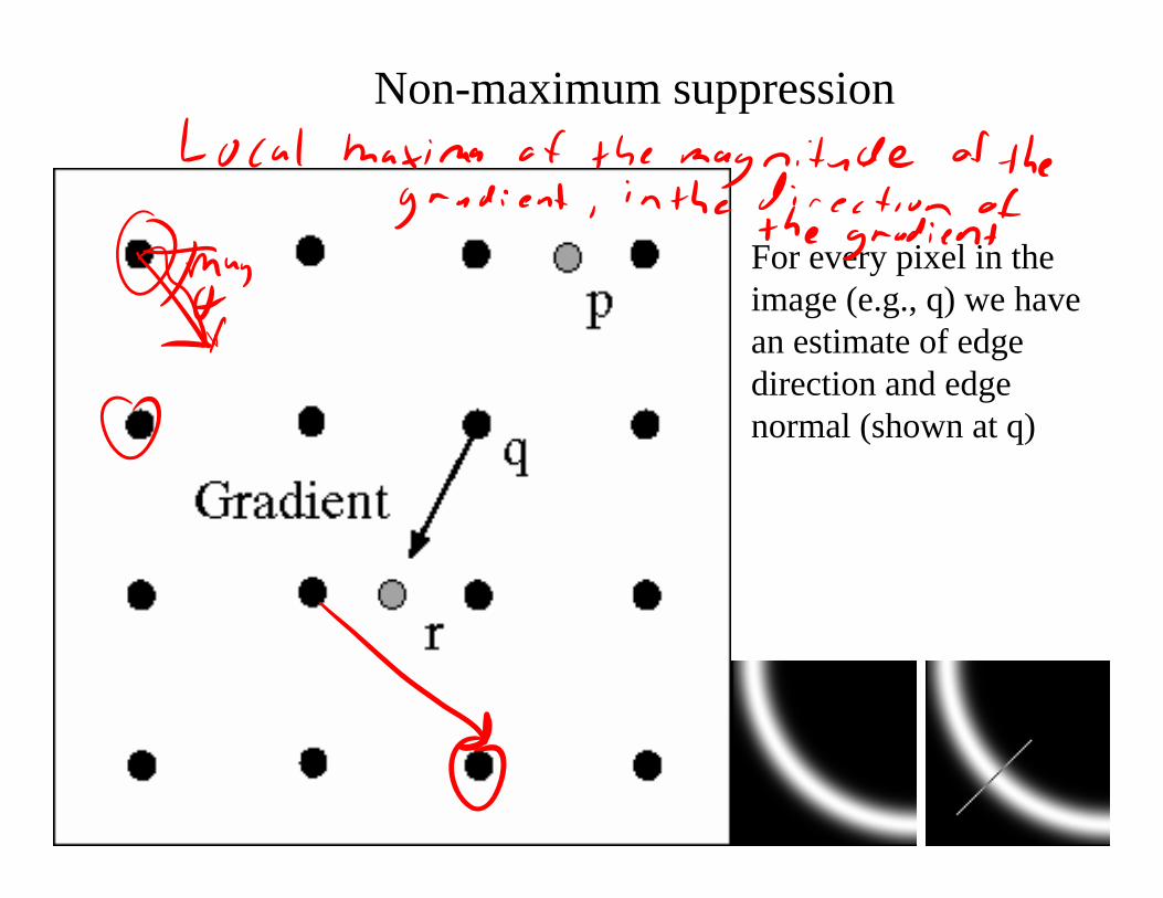
Non-maximum suppression

For every pixel in the image (e.g., q) we have an estimate of edge direction and edge normal (shown at q)


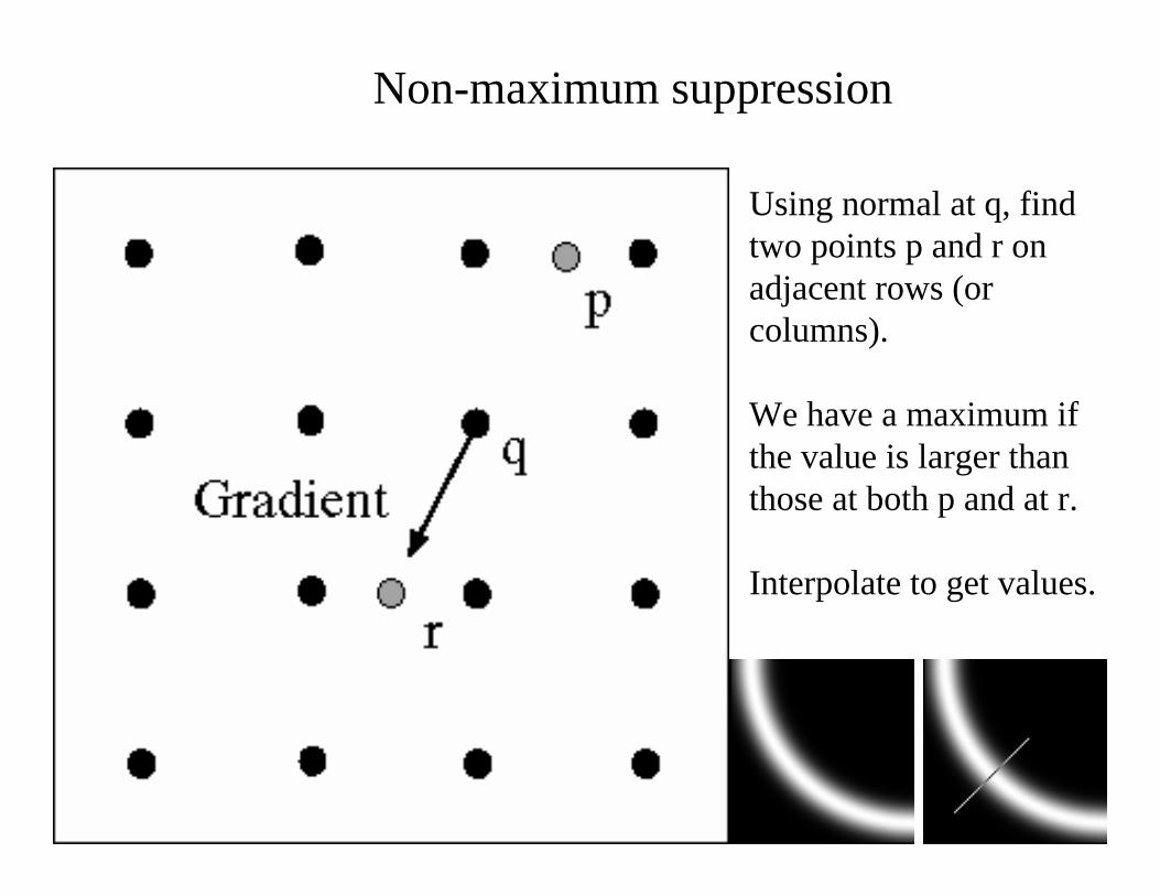
Non-maximum suppression

Using normal at q, find two points p and r on adjacent rows (or columns).

We have a maximum if the value is larger than those at both p and at r.

Interpolate to get values.


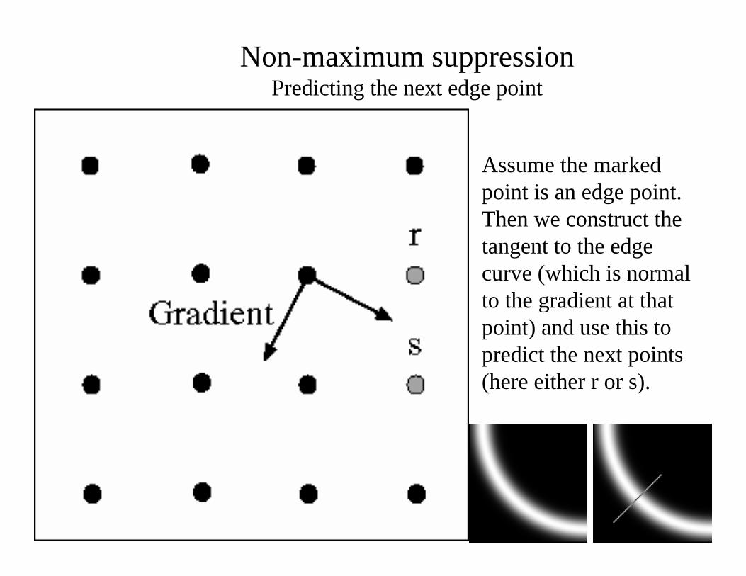
Assume the marked point is an edge point. Then we construct the tangent to the edge curve (which is normal to the gradient at that point) and use this to predict the next points (here either r or s).

Non-maximum suppressionPredicting the next edge point


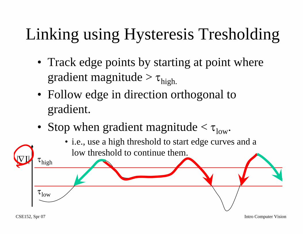
Linking using Hysteresis Tresholding• Track edge points by starting at point where

gradient magnitude > τhigh.

• Follow edge in direction orthogonal to gradient.

• Stop when gradient magnitude < τlow.• i.e., use a high threshold to start edge curves and a

low threshold to continue them.τhigh

τlow

|∇I|


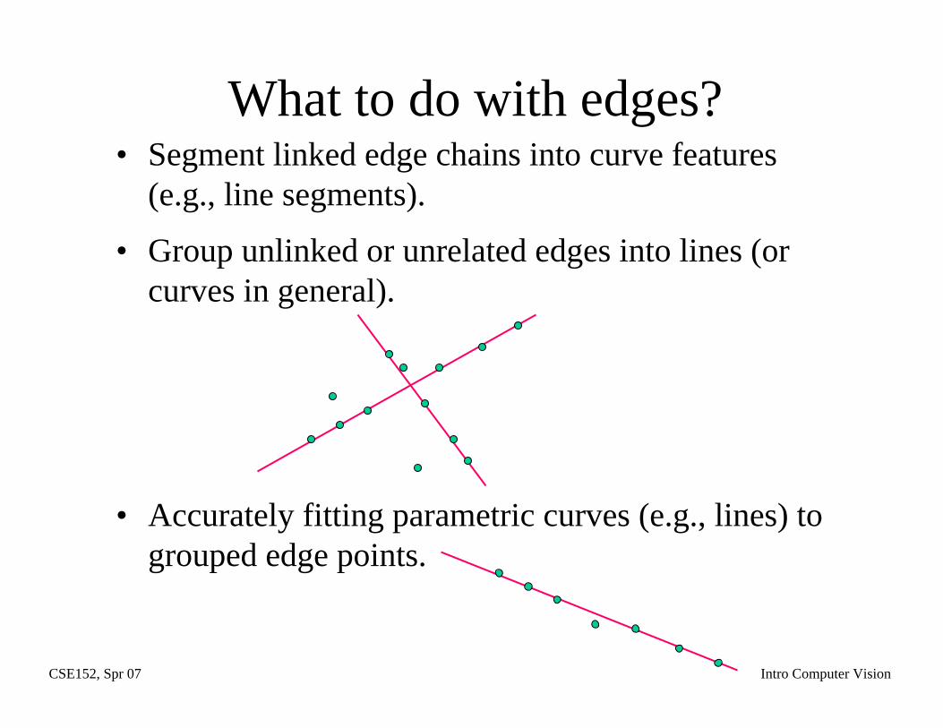
• Segment linked edge chains into curve features (e.g., line segments).

• Group unlinked or unrelated edges into lines (or curves in general).

• Accurately fitting parametric curves (e.g., lines) to grouped edge points.

What to do with edges?


Hough Transform[ Patented 1962 ]


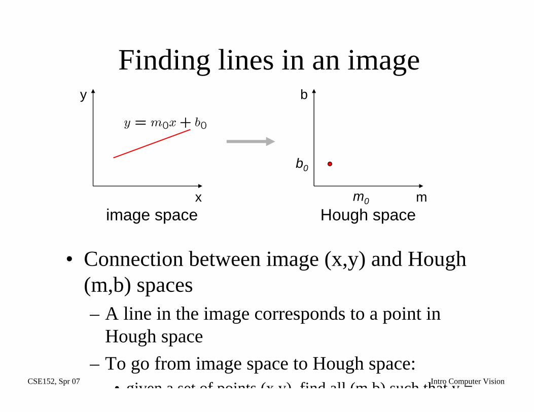
Finding lines in an image

• Connection between image (x,y) and Hough (m,b) spaces– A line in the image corresponds to a point in

Hough space– To go from image space to Hough space:

• given a set of points (x y) find all (m b) such that y =

x

y

m

b

m0

b0

image space Hough space


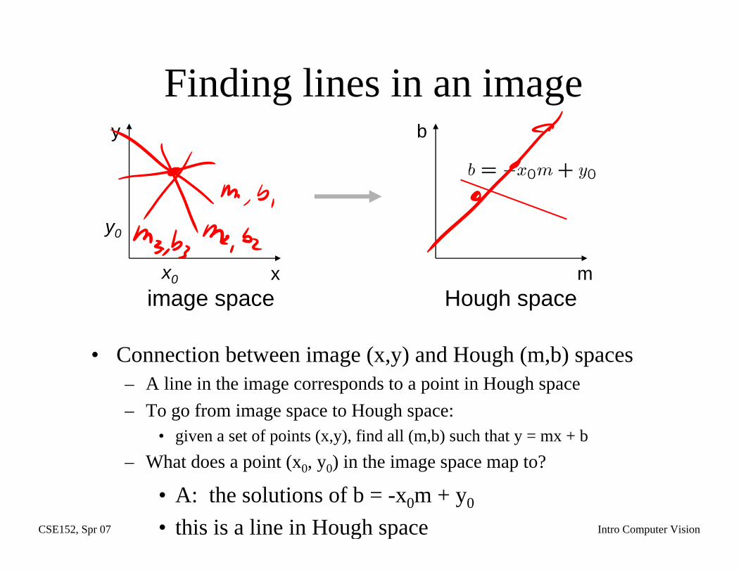
Finding lines in an image

• Connection between image (x,y) and Hough (m,b) spaces– A line in the image corresponds to a point in Hough space– To go from image space to Hough space:

• given a set of points (x,y), find all (m,b) such that y = mx + b– What does a point (x0, y0) in the image space map to?

x

y

m

b

image space Hough space

• A: the solutions of b = -x0m + y0

• this is a line in Hough space

x0

y0


Hough transform algorithm• Typically use a different parameterization

– d is the perpendicular distance from the line to the origin

– θ is the angle this perpendicular makes with the x axis

– Why?


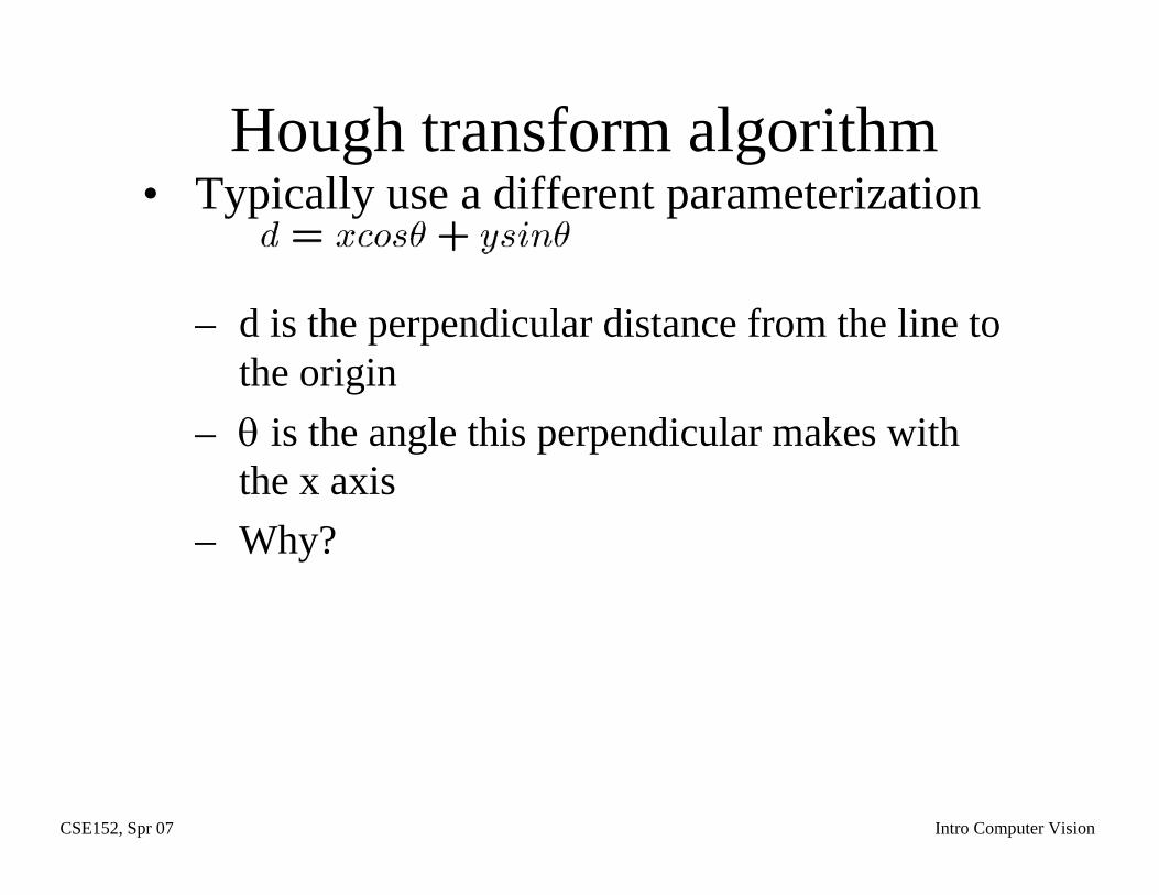
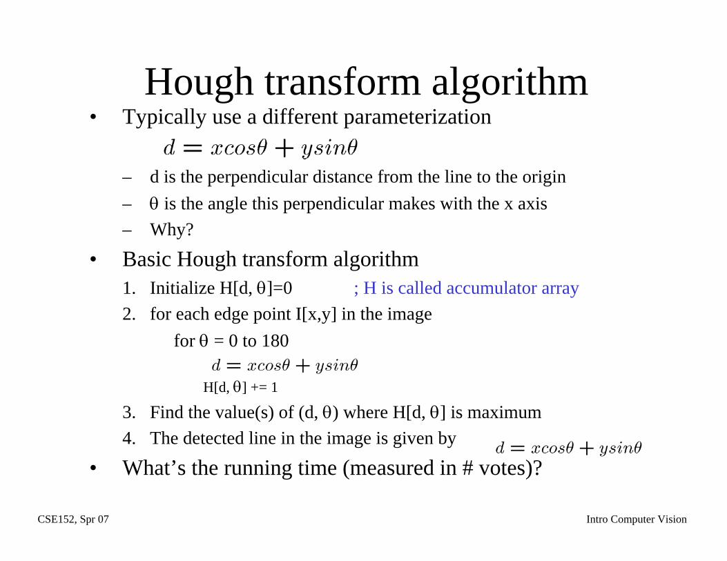
Hough transform algorithm• Typically use a different parameterization

– d is the perpendicular distance from the line to the origin– θ is the angle this perpendicular makes with the x axis– Why?

• Basic Hough transform algorithm1. Initialize H[d, θ]=0 ; H is called accumulator array2. for each edge point I[x,y] in the image

for θ = 0 to 180

H[d, θ] += 1

3. Find the value(s) of (d, θ) where H[d, θ] is maximum4. The detected line in the image is given by

• What’s the running time (measured in # votes)?


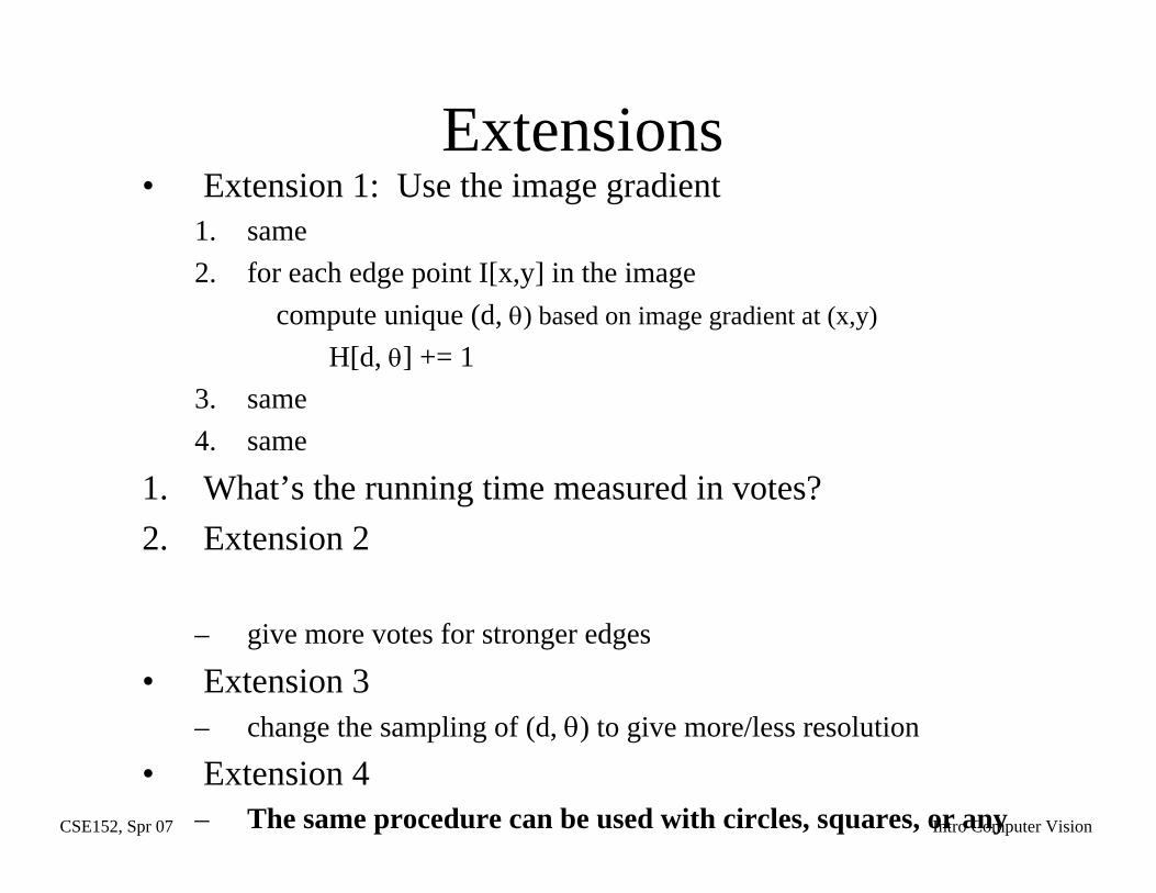
Extensions• Extension 1: Use the image gradient

1. same2. for each edge point I[x,y] in the image

compute unique (d, θ) based on image gradient at (x,y)H[d, θ] += 1

3. same4. same

1. What’s the running time measured in votes?2. Extension 2

– give more votes for stronger edges

• Extension 3– change the sampling of (d, θ) to give more/less resolution

• Extension 4– The same procedure can be used with circles, squares, or any


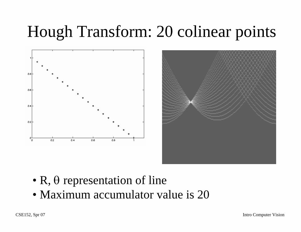
Hough Transform: 20 colinear points

• R, θ representation of line• Maximum accumulator value is 20


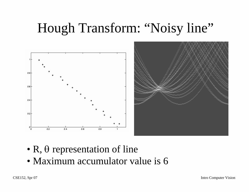
Hough Transform: “Noisy line”



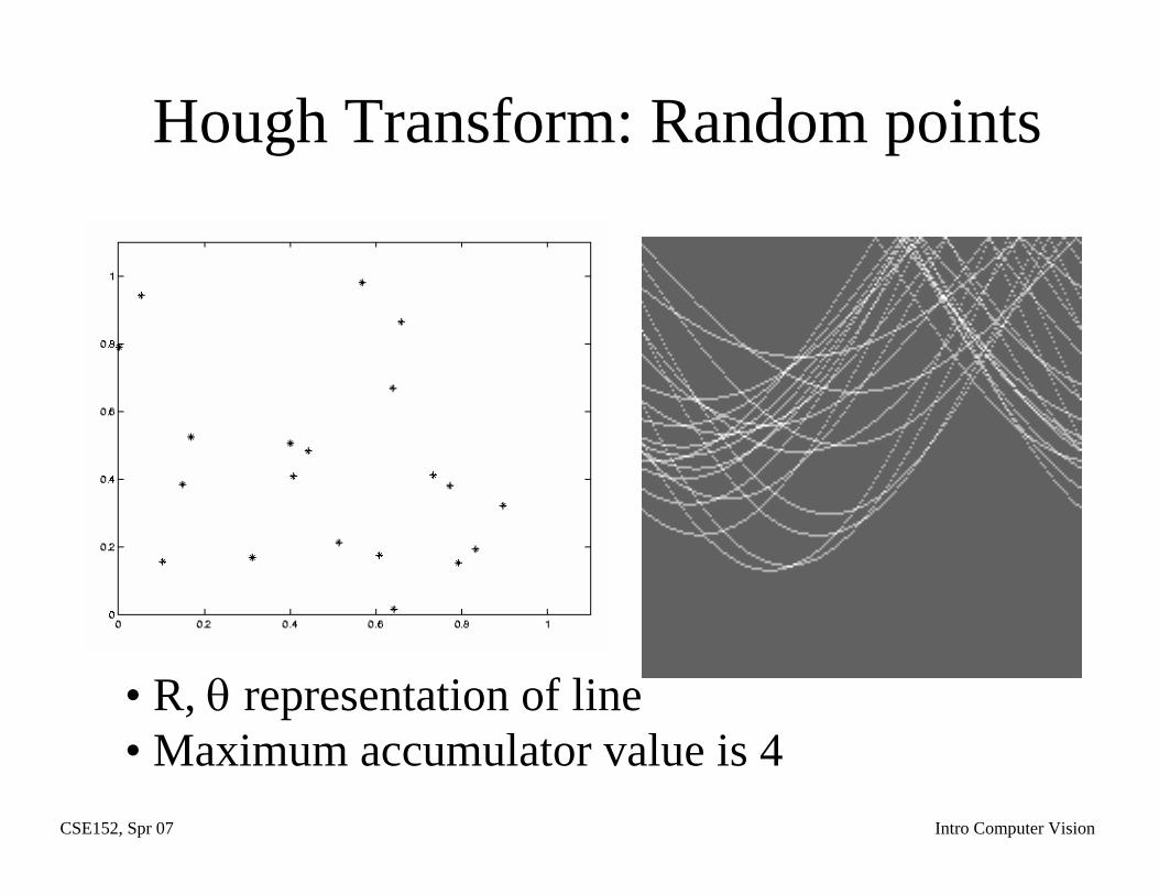
Hough Transform: Random points



Mechanics of the Hough transform• Difficulties

– how big should the cells be? (too big, and we cannot distinguish between quite different lines; too small, and noise causes lines to be missed)

• How many lines? – count the peaks in the Hough array

• Who belongs to which line?– tag the votes

• Complications, problems with noise and cell size


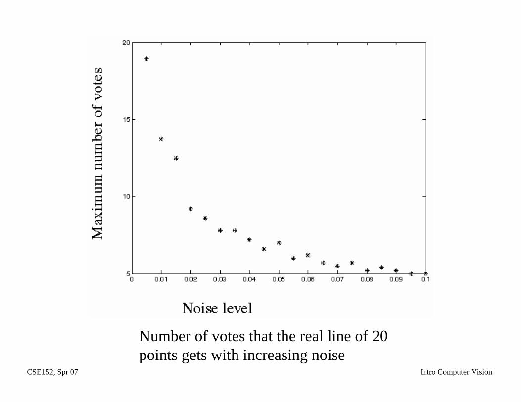
Number of votes that the real line of 20 points gets with increasing noise


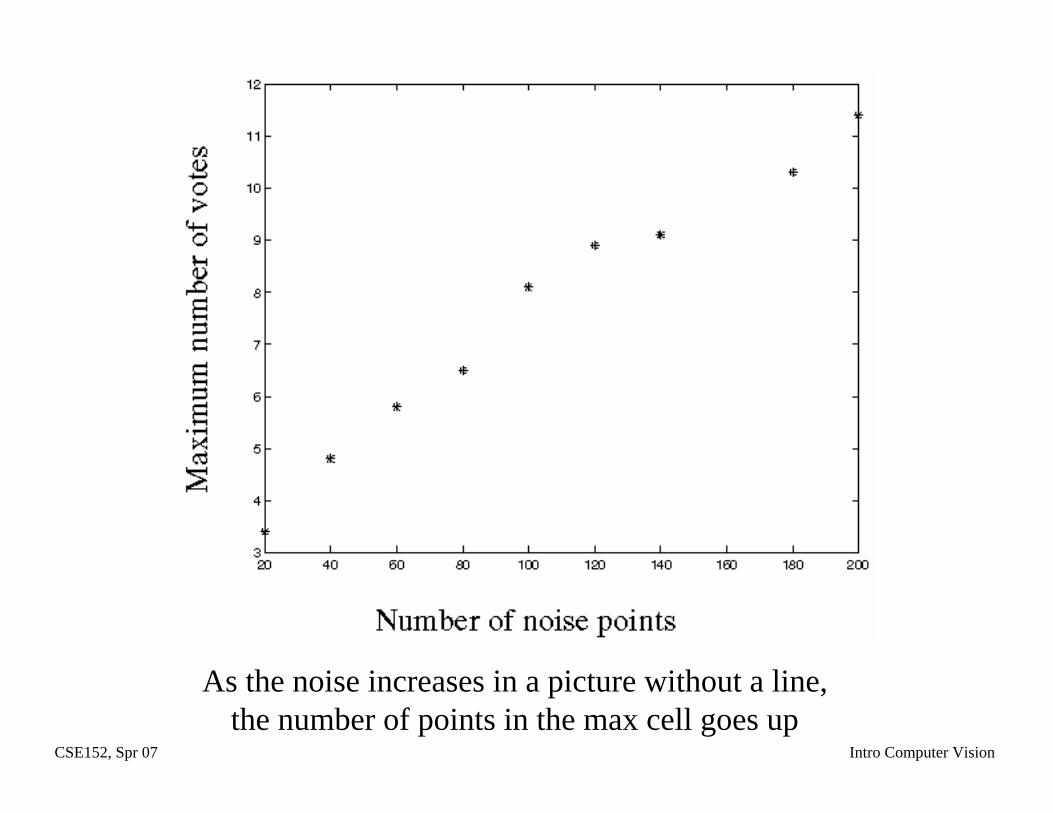
As the noise increases in a picture without a line, the number of points in the max cell goes up


Hough Transform for Curves(Generalized Hough Transform)

The H.T. can be generalized to detect any curve that can be expressed in parametric form:– Y = f(x, a1,a2,…ap)– Or g(x,y,a1,a2,…ap) = 0– a1, a2, … ap are the parameters– The parameter space is p-dimensional– The accumulating array is LARGE!


Example: Finding circlesEquation for circle is

(x – xc)2 + (y – yc)2 = r2

Where the parameters are the circle’s center (xc, yc) and radius r.

Three dimensional generalized Hough space.


• Work up circle example for next year


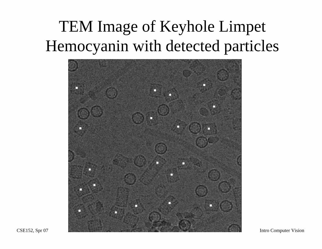
TEM Image of Keyhole Limpet Hemocyanin with detected particles


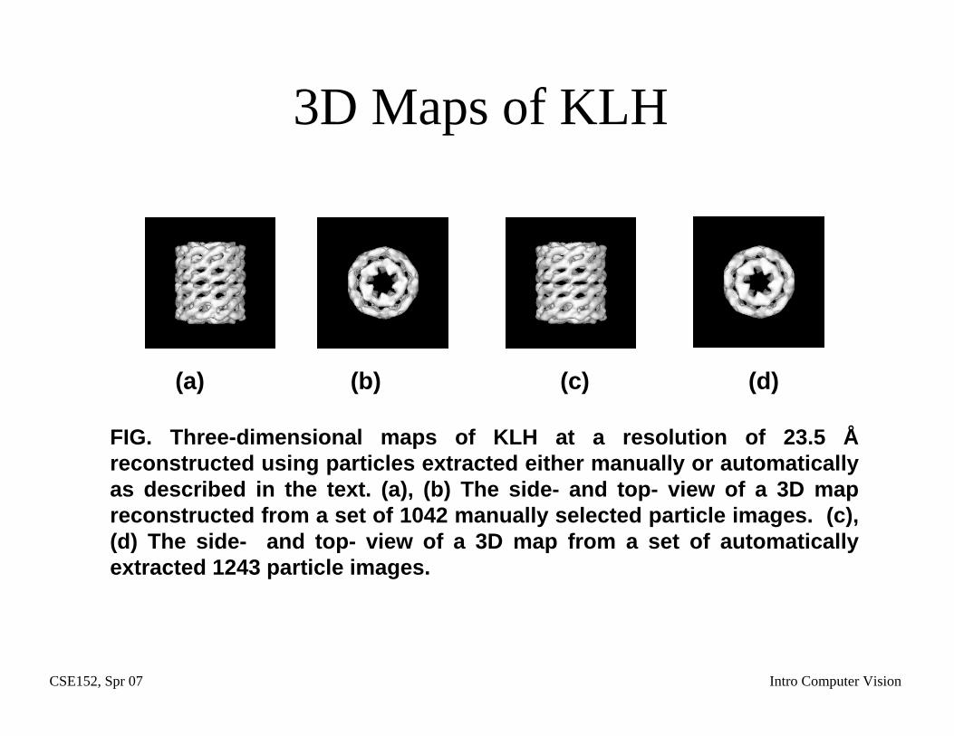
3D Maps of KLH

FIG. Three-dimensional maps of KLH at a resolution of 23.5 Åreconstructed using particles extracted either manually or automatically as described in the text. (a), (b) The side- and top- view of a 3D map reconstructed from a set of 1042 manually selected particle images. (c), (d) The side- and top- view of a 3D map from a set of automatically extracted 1243 particle images.

(a) (b) (c) (d)


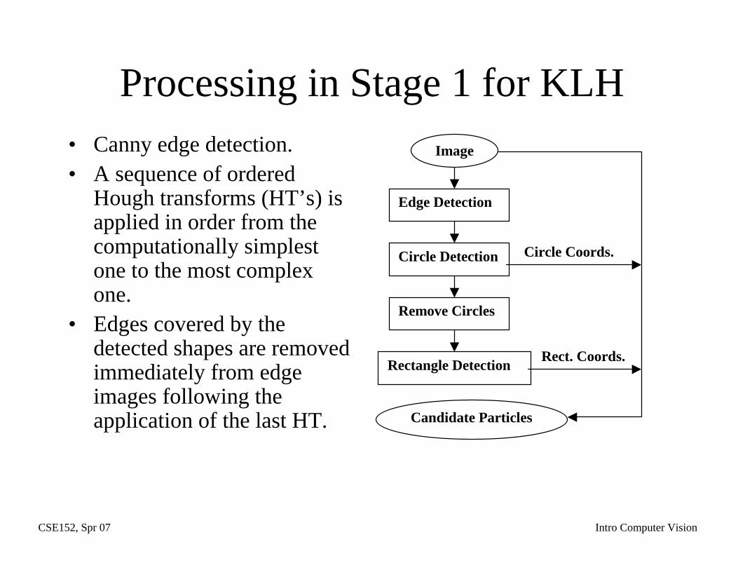
Processing in Stage 1 for KLH• Canny edge detection.• A sequence of ordered

Hough transforms (HT’s) is applied in order from the computationally simplest one to the most complex one.

• Edges covered by the detected shapes are removed immediately from edge images following the application of the last HT.

Edge Detection

Circle Detection

Remove Circles

Rectangle Detection

Image

Circle Coords.

Rect. Coords.

Candidate Particles


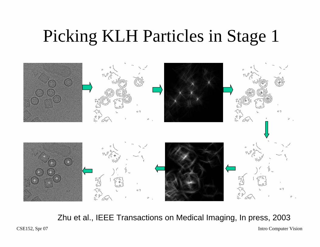
Picking KLH Particles in Stage 1

Zhu et al., IEEE Transactions on Medical Imaging, In press, 2003


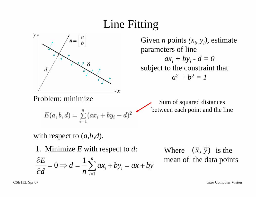
Line Fitting

Problem: minimize

with respect to (a,b,d).

1. Minimize E with respect to d:

Given n points (xi, yi), estimate parameters of line

axi + byi - d = 0subject to the constraint that

a2 + b2 = 1

Where is themean of the data points

) ,( yx

Sum of squared distances between each point and the line

ybxabyaxn

ddE n

iii +=+=⇒=

∂∂ ∑

=1

10


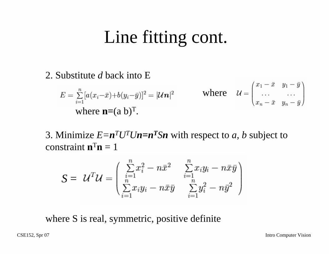
Line fitting cont.

2. Substitute d back into E

where n=(a b)T.

3. Minimize E=nTUTUn=nTSn with respect to a, b subject to constraint nTn = 1

where S is real, symmetric, positive definite

where

S =


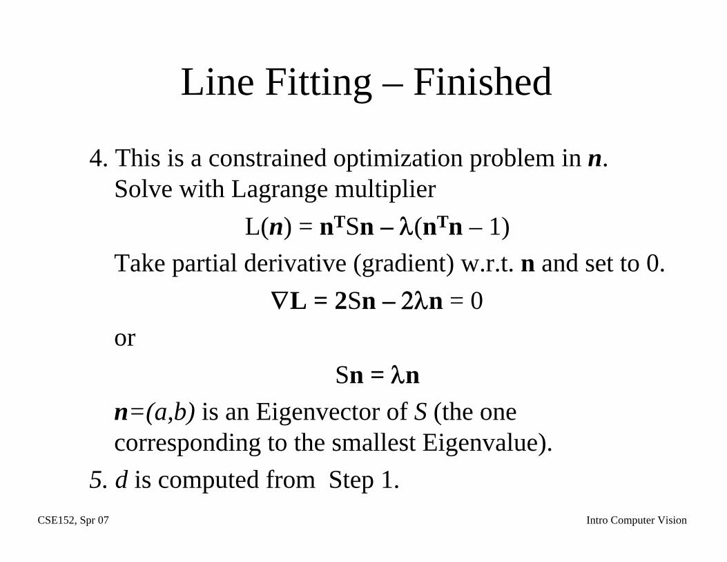
Line Fitting – Finished

4. This is a constrained optimization problem in n. Solve with Lagrange multiplier

L(n) = nTSn – λ(nTn – 1)Take partial derivative (gradient) w.r.t. n and set to 0.

∇L = 2Sn – 2λn = 0or

Sn = λnn=(a,b) is an Eigenvector of S (the one corresponding to the smallest Eigenvalue).

5. d is computed from Step 1.


MidtermThursday, May 10

• In class• Full period• Coverage – everything up to this point

including readings• “Cheat sheet” – you can prepare a one sided

sheet of notes. It must be hand written. (After the midterm, save your sheet since you can use the other side for the final).

• No calculators.


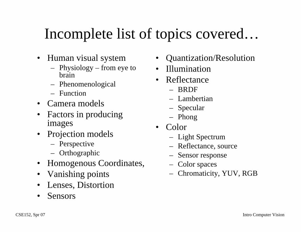
Incomplete list of topics covered…• Human visual system

– Physiology – from eye to brain

– Phenomenological– Function

• Camera models• Factors in producing

images• Projection models

– Perspective– Orthographic

• Homogenous Coordinates, • Vanishing points• Lenses, Distortion• Sensors

• Quantization/Resolution • Illumination• Reflectance

– BRDF– Lambertian– Specular– Phong

• Color– Light Spectrum– Reflectance, source– Sensor response– Color spaces– Chromaticity, YUV, RGB


Topics cont.• Binary Vision

– Thresholding– Neighborhoods– Connected component

exploration– Features, moments

• Noise– Additive, Gaussian noise

• Filtering, linear, convolution with Kernel– Averaging/smoothing– Sharpening– Derivatives– Gaussian filter– Seperability

• Edges & Edge detection• Edge sources• Canny

– Gaussian derivatives – Magnitude, orientation– Non-maximal suprression– Linking/thresholding

• Hough Transform• Generalized Hough

transform

Documents

Introduction to Computer Vision CSE 152 Lecture 11-a · CSE152, Spr 07 Intro Computer Vision Incomplete list of topics covered… • Human visual system – Physiology – from eye