Embed Size (px)
Citation preview
Introduction to Computational Physics
Lecture of Prof. H. J. Herrmann
Swiss Federal Institute of Technology ETH, Zürich, Switzerland
Script byDr. H. M. Singer, Lorenz Müller and Marco - Andrea Buchmann
Computational Physics, IfB, ETH Zürich

General Information
Useful Addresses and Information
The content of this class is available online on the following pages:
• http://www.comphys.ethz.ch/index.php/lectures
• http://www.ifb.ethz.ch/education/IntroductionComPhys
Pdf-files of both the slides and the exercises are also provided on these two pages.
Who is the Target Audience of This Lecture?
The lecture gives an introduction to computational physics for students of thefollowing departments:
• Mathematics and Computer Science (Bachelor and Master course)
• Physics (major course, “Wahlfach”)
• Material Science (Master course)
• Civil Engineering (Master course)
1

2
Some Words About Your Teacher
Prof. Hans. J. Herrmann is full professor at the Institute of Building Materials(IfB) since April 2006. His field of expertise is computational and statisticalphysics, in particular granular materials. His present research subjects includedense colloids, the formation of river deltas, quicksand, the failure of fibrous andpolymeric composites and complex networks.Prof. Herrmann can be reached at
His office is located in the Institute of Building materials (IfB), HIF E12, ETHHönggerberg, Zürich.The personal web page is located at www.icp.uni-stuttgart.de/~hans and atwww.comphys.ethz.ch
Some Words About the Authors
The script was started in 2007 by Dr. H.M. Singer, who wrote large parts of thechapter on random number generators, a part of the chapter on percolation, andlarge parts of the chapters on solving equations.
In 2009/2010, Lorenz Müller and Marco - Andrea Buchmann continued the scriptand filled in the gaps, expanded said chapters and added chapters on Monte Carlomethods, fractal dimensions and the Ising model.
If you have suggestions or corrections, please let us know:
Thank you!
Outline of This Course
This course consists of two parts:
In a first part we are going to consider stochastic processes, such as percola-tion. We shall look at random number generators, Monte Carlo methods and theIsing model, particularly their applications.
In the second part of the class we shall look into numerical ways of solving equa-tions (e.g. ordinary differential equations). We shall get to know a variety of waysto solve these and learn about their advantages as well as their disadvantages.

3
Prerequisites for this Class
• You should have a basic understanding of the UNIX operating system andbe able to work with it. This means concepts such as the ’shell’, streamredirections and compiling programs should be familiar.
• You should ideally have some knowledge about a higher level programminglanguage such as Fortran, C/C++, Java, ... . In particular you should alsobe able to write, compile and debug programs yourself.
• It is beneficial to know how to make scientific plots. There are many tools,which can help you with that. For example Matlab, Maple, Mathematica,R, SPlus, gnuplot, etc.
• Requirements in mathematics:
– You should know the basics of statistical analysis (averaging, distribu-tions, etc.).
– Furthermore, some knowledge of linear algebra and analysis will benecessary.
• Requirements in physics
– You should be familiar with Classical Mechanics (Newton, Lagrange)and Electrodynamics.
– A basic understanding of Thermodynamics is also beneficial.
Contents
I Stochastic Processes 8
1 Random Numbers 91.1 Definition of Random Numbers . . . . . . . . . . . . . . . . . . . 91.2 Congruential RNG (Multiplicative) . . . . . . . . . . . . . . . . . 101.3 Lagged Fibonacci RNG (Additive) . . . . . . . . . . . . . . . . . 131.4 How Good is a RNG? . . . . . . . . . . . . . . . . . . . . . . . . . 141.5 Non-Uniform Distributions . . . . . . . . . . . . . . . . . . . . . . 16
2 Percolation 222.1 The Sol-Gel Transition . . . . . . . . . . . . . . . . . . . . . . . . 232.2 The Percolation Model . . . . . . . . . . . . . . . . . . . . . . . . 23
3 Fractals 363.1 Self-Similarity . . . . . . . . . . . . . . . . . . . . . . . . . . . . . 363.2 Fractal Dimension: Mathematical Definition . . . . . . . . . . . . 373.3 The Box Counting Method . . . . . . . . . . . . . . . . . . . . . . 393.4 The Sandbox Method . . . . . . . . . . . . . . . . . . . . . . . . . 403.5 The Correlation-Function Method . . . . . . . . . . . . . . . . . . 413.6 Correlation Length ξ . . . . . . . . . . . . . . . . . . . . . . . . . 423.7 Finite Size Effects . . . . . . . . . . . . . . . . . . . . . . . . . . . 433.8 Fractal Dimension in Percolation . . . . . . . . . . . . . . . . . . 463.9 Examples . . . . . . . . . . . . . . . . . . . . . . . . . . . . . . . 463.10 Cellular Automata . . . . . . . . . . . . . . . . . . . . . . . . . . 47
4 Monte Carlo Methods 514.1 What is “Monte Carlo” ? . . . . . . . . . . . . . . . . . . . . . . . 514.2 Applications of Monte Carlo . . . . . . . . . . . . . . . . . . . . . 514.3 Computation of Integrals . . . . . . . . . . . . . . . . . . . . . . . 534.4 Higher Dimensional Integrals . . . . . . . . . . . . . . . . . . . . . 574.5 Canonical Monte Carlo . . . . . . . . . . . . . . . . . . . . . . . . 584.6 The Ising Model . . . . . . . . . . . . . . . . . . . . . . . . . . . . 674.7 Interfaces . . . . . . . . . . . . . . . . . . . . . . . . . . . . . . . 704.8 Simulation Examples . . . . . . . . . . . . . . . . . . . . . . . . . 81
4
CONTENTS 5
II Solving Systems of Equations Numerically 83
5 Solving Equations 845.1 One-Dimensional Case . . . . . . . . . . . . . . . . . . . . . . . . 845.2 N -Dimensional Case . . . . . . . . . . . . . . . . . . . . . . . . . 87
6 Ordinary Differential Equations 896.1 Examples . . . . . . . . . . . . . . . . . . . . . . . . . . . . . . . 896.2 Euler Method . . . . . . . . . . . . . . . . . . . . . . . . . . . . . 896.3 Runge-Kutta Methods . . . . . . . . . . . . . . . . . . . . . . . . 92
7 Partial Differential Equations 1047.1 Types of PDEs . . . . . . . . . . . . . . . . . . . . . . . . . . . . 1047.2 Examples of PDEs . . . . . . . . . . . . . . . . . . . . . . . . . . 1057.3 Discretization of the Derivatives . . . . . . . . . . . . . . . . . . . 1097.4 The Poisson Equation . . . . . . . . . . . . . . . . . . . . . . . . 1107.5 Solving Systems of Linear Equations . . . . . . . . . . . . . . . . 1127.6 Finite Element Method . . . . . . . . . . . . . . . . . . . . . . . . 1277.7 Time Dependent PDEs . . . . . . . . . . . . . . . . . . . . . . . . 1397.8 Discrete Fluid Solver . . . . . . . . . . . . . . . . . . . . . . . . . 147
CONTENTS 6
What is Computational Physics?
Computational physics is the study and implementation of numerical algorithmsto solve problems in physics by means of computers. Computational physics inparticular solves equations numerically. Finding a solution numerically is useful,as there are very few systems for which an analytical solution is known. Anotherfield of computational physics is the simulation of many-body/particle systems;in this area, a virtual reality is created which is sometimes also referred to as the3rd branch of physics (between experiments and theory).
The evaluation and visualization of large data sets, which can come from nu-merical simulations or experimental data (for example maps in geophysics) is alsopart of computational physics.
Another area in which computers are used in physics is the control of experi-ments. However, this area is not treated in the lecture.
Computational physics plays an important role in the following fields:
• Computational Fluid Dynamics (CFD): solve and analyze problems thatinvolve fluid flows
• Classical Phase Transition: percolation, critical phenomena
• Solid State Physics (Quantum Mechanics)
• High Energy Physics / Particle Physics: in particular Lattice QuantumChromodynamics (“Lattice QCD”)
• Astrophysics: many-body simulations of stars, galaxies etc.
• Geophysics and Solid Mechanics: earthquake simulations, fracture, rupture,crack propagation etc.
• Agent Models (interdisciplinary): complex networks in biology, economy,social sciences and many others
CONTENTS 7
Suggested Literature
Books:
• H. Gould, J. Tobochnik and Wolfgang Christian: „Introduction to ComputerSimulation Methods“ 3rd edition (Addison Wesley, Reading MA, 2006).
• D. P. Landau and K. Binder: „A Guide to Monte Carlo Simulations inStatistical Physics“ (Cambridge University Press, Cambridge, 2000).
• D. Stauffer, F. W. Hehl, V. Winkelmann and J. G. Zabolitzky: „ComputerSimulation and Computer Algebra“ 3rd edition (Springer, Berlin, 1993).
• K. Binder and D. W. Heermann: „Monte Carlo Simulation in StatisticalPhysics“ 4th edition (Springer, Berlin, 2002).
• N. J. Giordano: „Computational Physics“ (Addison Wesley, Reading MA,1996).
• J. M. Thijssen: “Computational Physics”, (Cambridge University Press,Cambridge, 1999).
Book Series:
• „Monte Carlo Method in Condensed Matter Physics“, ed. K. Binder (SpringerSeries).
• „Annual Reviews of Computational Physics“, ed. D. Stauffer (World Scien-tific).
• „Granada Lectures in Computational Physics“, ed. J. Marro (Springer Se-ries).
• „Computer Simulations Studies in Condensed Matter Physics“, ed. D. Lan-dau (Springer Series).
Journals:
• Journal of Computational Physics (Elsevier).
• Computer Physics Communications (Elsevier).
• International Journal of Modern Physics C (World Scientific).
Conferences:
• Annual Conference on Computational Physics (CCP): In 2007, the CCPwas held in Brussels (Sept. 5th-8th 2007), in 2008 it was in Brazil.

Part I
Stochastic Processes
8
Chapter 1
Random Numbers
Random numbers (RN) are an important tool for scientific simulations. As weshall see in this class, they are used in many different applications, including thefollowing:
• Simulate random events and experimental fluctuations, for example radioac-tive decay
• Complement the lack of detailed knowledge (e.g. traffic or stock marketsimulations)
• Consider many degrees of freedom (e.g. Brownian motion, random walks).
• Test the stability of a system with respect to perturbations
• Random sampling
Special literature about random numbers is given at the end of this chapter.
1.1 Definition of Random NumbersRandom numbers are a sequence of numbers in random or uncorrelated order.In particular, the probability that a given number occurs next in the sequenceis always the same. Physical systems can produce random events, for examplein electronic circuits (“electronic flicker noise”) or in systems where quantum ef-fects play an important role (such as for example radioactive decay or the photonemission from a semiconductor). However, physical random numbers are usually“bad” in the sense that they are usually correlated.
The algorithmic creation of random numbers is a bit problematic, since the com-puter is completely deterministic but the sequence should be non-deterministic.One therefore considers the creation of pseudo-random numbers, which are cal-culated with a deterministic algorithm, but in such a way that the numbers are
9
CHAPTER 1. RANDOM NUMBERS 10
almost homogeneously, randomly distributed. These numbers should follow awell-defined distribution and should have long periods. Furthermore, they shouldbe calculated quickly and in a reproducible way.
A very important tool in the creation of pseudo-random numbers is the modulo-operator mod (in C++ %), which determines the remainder of a division of oneinteger number with another one.
Given two numbers a (dividend) and n (divisor), we write amodulon or amodnwhich stands for the remainder of division of a by n. The mathematical definitionof this operator is as follows: We consider a number q ∈ Z, and the two integersa and n mentioned previously. We then write a as
a = nq + r (1.1)
with 0 ≤ r < |n|, where r is the the remainder. The mod-operator is useful be-cause one obtains both big and small numbers when starting with a big number.
The pseudo-random number generators (RNG) can be divided into two classes:the multiplicative and the additive generators.
• The multiplicative ones are simpler and faster to program and execute, butdo not produce very good sequences.
• The additive ones are more difficult to implement and take longer to run,but produce much better random sequences.
1.2 Congruential RNG (Multiplicative)The simplest form of a congruential RNG was proposed by Lehmer in 1948. Thealgorithm is based on the properties of the mod-operator. Let us assume that wechoose two integer numbers c and p and a seed value x0 with c, p, x0 being positiveintegers. We then create the sequence {xi}, i ∈ N, iteratively by the recurrencerelation
xi = (cxi−1)mod p, (1.2)
which creates random numbers in the interval [0, p − 1] 1. In order to transformthese random numbers to the interval [0, 1[ we simply divide by p
0 ≤ zi =xip< 1 (1.3)
1Throughout the manuscript we will adopt the notation that closed square brackets [ ] inintervals are equivalent to ≤ and ≥ and open brackets ] [ correspond to < and > respectively.Thus the interval [0, 1] corresponds to 0 ≤ x ≤ 1, x ∈ R and ]0, 1] means 0 < x ≤ 1, x ∈ R.
CHAPTER 1. RANDOM NUMBERS 11
with zi ∈ R (actually zi ∈ Q).
Since all integers are smaller than p the sequence must repeat after at least (p−1)iterations. Thus, the maximal period of this RNG is (p− 1). If we pick the seedvalue x0 = 0, the sequence sits on a fixed point 0 (therefore, x0 = 0 cannot beused).
In 1910, R. D. Carmichael proved that the maximal period can be obtained ifp is a Mersenne prime number2 and if the number is at the same time the smallestinteger number for which the following condition holds:
cp−1 mod p = 1. (1.4)
In 1988, Park and Miller presented the following numbers, which produce a rela-tively long sequence of pseudo-random numbers, here in pseudo-C code:
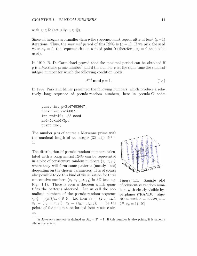
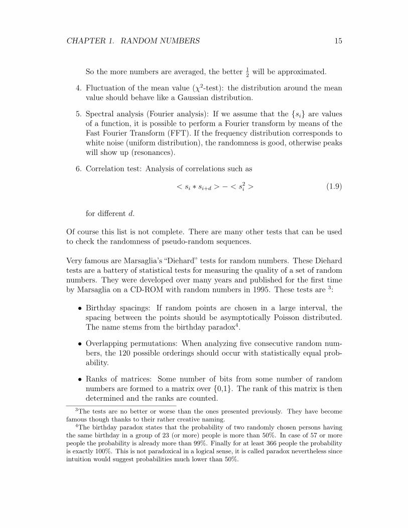
Figure 1.1: Sample plotof consecutive random num-bers with clearly visible hy-perplanes (“RANDU” algo-rithm with c = 65539, p =231, x0 = 1) [20]
const int p=2147483647;const int c=16807;int rnd=42; // seedrnd=(c*rnd)%p;print rnd;
The number p is of course a Mersenne prime withthe maximal length of an integer (32 bit): 231 −1.
The distribution of pseudo-random numbers calcu-lated with a congruential RNG can be representedin a plot of consecutive random numbers (xi, xi+1),where they will form some patterns (mostly lines)depending on the chosen parameters. It is of coursealso possible to do this kind of visualization for threeconsecutive numbers (xi, xi+1, xi+2) in 3D (see e.g.Fig. 1.1). There is even a theorem which quan-tifies the patterns observed. Let us call the nor-malized numbers of the pseudo-random sequence{zi} = {xi}/p, i ∈ N. Let then π1 = (z1, ..., zn),π2 = (z2, ..., zn+1), π3 = (z3, ..., zn+2), ... be thepoints of the unit n-cube formed from n successivezi.
2A Mersenne number is defined as Mn = 2n − 1. If this number is also prime, it is called aMersenne prime.
CHAPTER 1. RANDOM NUMBERS 12
Theorem 1 (Marsaglia, 1968). If a1, a2, ..., an ∈ Zis any choice of integers such that
a1 + a2c+ a3c2 + ...+ anc
n−1 ≡ 0mod p,
then all of the points π1, π2, ... will lie in the set of parallel hyperplanes defined bythe equations
a1y1 + a2y2 + ...+ anyn = 0,±1,±2, ..., yi ∈ R, 1 ≤ i ≤ n
There are at most|a1|+ |a2|+ ...+ |an|
of these hyperplanes, which intersect the unit n-cube and there is always a choiceof a1, ..., an such that all of the points fall in fewer than (n!p)1/n hyperplanes.
Proof. (Abbreviated) The theorem is proved in four steps: Step 1 : If
a1 + a2c+ a3c2 + ...+ anc
n−1 ≡ 0mod p
then one can prove that
a1zi + a2zi+1 + ...+ anzi+n−1
is an integer for every i and thusStep 2 : The point πi = (zi, zi+1, .., zi+n−1) must lie in one of the hyperplanes
a1y1 + a2y2 + ...+ anyn = 0,±1,±2, ..., yi ∈ R, 1 ≤ i ≤ n.
Step 3 : The number of hyperplanes of the above type, which intersect the unitn-cube is at most
|a1|+ |a2|+ ...+ |an|,andStep 4 : For every multiplier c and modulus p there is a set of integers a1, ..., an(not all zero) such that
a1 + a2c+ a3c2 + ...+ anc
n−1 ≡ 0mod p
and|a1|+ |a2|+ ...+ |an| ≤ (n!p)1/n.
This is of course only the outline of the proof. The exact details can be read inG. Marsaglia, Proc. Nat. Sci. U.S.A. 61, 25 (1968).
In a very similar way it is possible to show that for congruential RNGs the distancebetween the planes must be larger than√
p
n(1.5)
CHAPTER 1. RANDOM NUMBERS 13
1.3 Lagged Fibonacci RNG (Additive)A more complicated version of a RNG is the Lagged Fibonacci algorithm proposedby Tausworth in 1965. Lagged Fibonacci type generators permit extremely largeperiods and even allow for advantageous predictions about correlations.
Lagged Fibonacci generators often use integer values, but in the following weshall focus on binary values.
Consider a sequence of of binary numbers xi ∈ {0, 1}, 1 ≤ i ≤ b. The nextbit in our sequence, xb+1 is then given by
xb+1 = (∑j∈J
xb+1−j)mod 2 (1.6)
with J ⊂ [1, .., b]. In other words, the sum includes only a subset of all the otherbits, so the new bit could for instance simply be based on the first and third bit,xb+1 = (x1 + x3)mod 2 (or of course any other subset!).
Let us try to illustrate some points with a two element lagged Fibonacci gen-erator. Consider two natural numbers c, d ∈ N with d ≤ c, and we define oursequence recursively as
xi+1 = (xi−c + xi−d)mod 2
Of course we immediately see that we need some initial sequence of at least cbits to start from (a so-called seed sequence). One usually uses a congruentialgenerator to obtain the seed sequence.
Much as in the case of congruential generators, there are conditions for the choiceof the numbers c and d. In this case, c and d must satisfy the Zierler-Trinomialcondition which states that
Tc,d(z) = 1 + zc + zd (1.7)
cannot be factorized in subpolynomials, where z is a binary number. The numberc is chosen up to 100, 000 and it can be shown that the maximal period is 2c − 1,which is much larger than for congruential generators. The smallest numberssatisfying the Zierler conditions are (c, d) = (250, 103). The generator is namedafter the discoverers of the numbers, Kirkpatrick and Stoll (1981).
CHAPTER 1. RANDOM NUMBERS 14
The following pairs (c, d) are known:
(c, d)
(250 , 103) Kirkpatrick− Stoll (1981)
(4187 , 1689) J.R.Heringa et al. (1992)
(132049 , 54454)
(6972592 , 3037958) R.P.Brent et al. (2003)
1.3.1 Implementation
There are two methods to convert the obtained binary sequences to natural num-bers (e.g. 32 bit unsigned variables):
• One runs 32 Fibonacci generators in parallel (this can be done very ef-ficiently). The problem with this method is the initialization, as the 32initial sequences do not only need to be uncorrelated each one by itself butalso among each other. The quality of the initial sequences has a majorimpact on the quality of the produced random numbers.
• One extracts a 32 bit long part from the sequence. This method is relativelyslow, as for each random number one needs to generate 32 new elements inthe binary sequence. Furthermore, it has been shown that random numbersproduced in this way show strong correlations.
1.4 How Good is a RNG?There are many possibilities to test how random a sequence generated by a givenRNG really is. There is an impressive collection of possible tests for a givensequence {si}, i ∈ N, for instance:
1. Square test: the plot of two consecutive numbers (si, si+1)∀i should bedistributed homogeneously. Any sign of lines or clustering shows the non-randomness and correlation of the sequence {si}.
2. Cube test: this test is similar to the square test, but this time the plot isthree-dimensional with the tuples (si, si+1, si+2). Again the tuples should bedistributed homogeneously.
3. Average value: the arithmetic mean of all the numbers in the sequence {si}should correspond to the analytical mean value. Let us assume here thatthe numbers si are rescaled to be in the interval si ∈ [0, 1[. The arithmeticmean should then be
s = limN→∞
1
N
N∑i=1
si =1
2(1.8)
CHAPTER 1. RANDOM NUMBERS 15
So the more numbers are averaged, the better 12will be approximated.
4. Fluctuation of the mean value (χ2-test): the distribution around the meanvalue should behave like a Gaussian distribution.
5. Spectral analysis (Fourier analysis): If we assume that the {si} are valuesof a function, it is possible to perform a Fourier transform by means of theFast Fourier Transform (FFT). If the frequency distribution corresponds towhite noise (uniform distribution), the randomness is good, otherwise peakswill show up (resonances).
6. Correlation test: Analysis of correlations such as
< si ∗ si+d > − < s2i > (1.9)
for different d.
Of course this list is not complete. There are many other tests that can be usedto check the randomness of pseudo-random sequences.
Very famous are Marsaglia’s “Diehard” tests for random numbers. These Diehardtests are a battery of statistical tests for measuring the quality of a set of randomnumbers. They were developed over many years and published for the first timeby Marsaglia on a CD-ROM with random numbers in 1995. These tests are 3:
• Birthday spacings: If random points are chosen in a large interval, thespacing between the points should be asymptotically Poisson distributed.The name stems from the birthday paradox4.
• Overlapping permutations: When analyzing five consecutive random num-bers, the 120 possible orderings should occur with statistically equal prob-ability.
• Ranks of matrices: Some number of bits from some number of randomnumbers are formed to a matrix over {0,1}. The rank of this matrix is thendetermined and the ranks are counted.
3The tests are no better or worse than the ones presented previously. They have becomefamous though thanks to their rather creative naming.
4The birthday paradox states that the probability of two randomly chosen persons havingthe same birthday in a group of 23 (or more) people is more than 50%. In case of 57 or morepeople the probability is already more than 99%. Finally for at least 366 people the probabilityis exactly 100%. This is not paradoxical in a logical sense, it is called paradox nevertheless sinceintuition would suggest probabilities much lower than 50%.
CHAPTER 1. RANDOM NUMBERS 16
• Monkey test: Sequences of some number of bits are taken as words and thenumber of overlapping words in a stream is counted. The number of wordsnot appearing should follow a known distribution. The name is based onthe infinite monkey theorem5.
• Parking lot test: Randomly place unit circles in a 100 x 100 square. If thecircle overlaps an existing one, try again. After 12,000 tries, the number ofsuccessfully "parked" circles should follow a certain normal distribution.
• Minimum distance test: Find the minimum distance of 8000 randomlyplaced points in a 10000 x 10000 square. The square of this distance shouldbe exponentially distributed with a certain mean.
• Random spheres test: put 4000 randomly chosen points in a cube of edge1000. Now a sphere is placed on every point with a radius correspondingto the minimum distance to another point. The smallest sphere’s volumeshould then be exponentially distributed.
• Squeeze test: 231 is multiplied by random floats in [0, 1[ until 1 is reached.After 100,000 repetitions the number of floats needed to reach 1 shouldfollow a certain distribution.
• Overlapping sums test: Sequences of 100 consecutive floats are summedup in a very long sequence of random floats in [0, 1[. The sums should benormally distributed with characteristic mean and standard deviation.
• Runs test: Ascending and descending runs in a long sequence of randomfloats in [0, 1[ are counted. The counts should follow a certain distribution.
• Craps test: 200,000 games of craps6 are played. The number of wins andthe number of throws per game should follow a certain distribution.
1.5 Non-Uniform DistributionsWe have so far only considered the uniform distribution of pseudo-random num-bers. The congruential and lagged Fibonacci RNG produce numbers in N whichcan easily be mapped to the interval [0, 1[ or any other interval by simple shiftsand multiplications. However, if the goal is to produce random numbers whichare distributed according to a certain distribution (e.g. Gaussian), the algorithmspresented so far are not very well suited. There are however tricks that permit us
5The infinite monkey theorem states that a monkey hitting keys at random on a typewriterkeyboard for an infinite amount of time will almost surely (i.e. with probability 1) type aparticular chosen text, such as the complete works of William Shakespeare.
6Dice game
CHAPTER 1. RANDOM NUMBERS 17
to transform uniform pseudo-random numbers to other distributions. There areessentially two different ways to perform this transformation:
• If we are looking at a distribution whose analytic description is known, itmay be possible to apply a mapping
• However, if the analytic description is unknown (or the transformation can-not be applied), we have to use the so-called rejection method.
These methods are explained in the following sections.
1.5.1 Transformation Methods of Special Distributions
For a certain class of distributions it is possible to create pseudo-random numbersfrom uniformly distributed random numbers by finding a mathematical trans-formation. The transformation method works particularly nicely for the mostcommon distributions (exponential, Poisson and normal distribution). While thetransformation is rather straightforward, it is not always feasible - this depends onthe analytical description of the distribution. The idea is to find the equivalencebetween area slices of the uniform distribution Pu and the distribution of interest.The uniform distribution is written as
Pu(z) =
{1 for z ∈ [0, 1]0 otherwise
(1.10)
Let us now consider the distribution P (y). If we compare the areas of intergration,we find
z =
ˆ y
0
P (y′)dy′ =
ˆ z
0
Pu(z′)dz′ (1.11)
where z is a uniformly distributed random variable and y a random variabledistributed according to the desired distribution. Let us rewrite the integral ofP (y) as IP (y) then we find z = IP (y) and therefore
y = I−1P (z) (1.12)
This shows that a transformation between the two distributions can be found onlyif
1. the integral IP (y) =´ y
0P (y′)dy′ can be solved analytically in a closed form
2. there exists an analytic inverse of z = IP (y) such that y = I−1P (z)
Of course, these conditions can be overcome to a certain extent by precalculat-ing/tabulating and inverting IP (y) numerically, if the integral is well-behaved (i.e.is non-singular). Then, with a little help from precalculated tables, it is possibleto transform the uniform numbers numerically.
CHAPTER 1. RANDOM NUMBERS 18
We are now going to demonstrate this method for the two most commonly useddistributions: the Poisson distribution and the Gaussian distribution. We arealready going to see in the case of the Gaussian distribution that quite a bit ofwork is required to create such a transformation.
The Poisson Distribution
The Poisson distribution is defined as
P (y) = ke−yk. (1.13)
By applying the area equality of eq. (1.11) we find
z =
ˆ y
0
ke−y′kdy′ =
ˆ z
0
Pu(z′)dz′ (1.14)
thusz = −e−y′k|y0 = 1− e−yk. (1.15)
Solving for y yields
y = −1
kln(1− z). (1.16)
The Gaussian Distribution
Analytical methods of generating normally distributed random number are veryuseful, since there are many applications and examples where such numbers areneeded.
The Gaussian or normal distribution is written as
P (y) =1√πσ
e−y2
σ (1.17)
Unfortunately, only the limit for y →∞ can be solved analytically:ˆ ∞0
1√πσ
e−y′2σ dy′ =
√π
2. (1.18)
However, Box and Muller7 have introduced the following elegant trick to circum-vent this restriction. Let us assume we take two (uncorrelated) uniform randomvariables z1 and z2. Of course we can apply the area equality of eq. (1.11) againbut this time we write it as a product of the two random variables
z1 · z2 =
ˆ y1
0
1√πσ
e−y′21σ dy′1 ·
ˆ y2
0
1√πσ
e−y′22σ dy′2 =
ˆ y2
0
ˆ y1
0
1
πσe−
y′21+y′22σ dy′1dy
′2.
(1.19)7G. E. P. Box and Mervin E. Muller, A Note on the Generation of Random Normal Deviates,
The Annals of Mathematical Statistics (1958), Vol. 29, No. 2 pp. 610-611
CHAPTER 1. RANDOM NUMBERS 19
This integral can now be solved by transforming the variables y′1 and y′2 into polarcoordinates:
r2 = y21 + y2
2 (1.20)
tanφ =y1
y2
(1.21)
withdy′1dy
′2 = r′dr′dφ′ (1.22)
Substituting in eq. (1.19) leads to
z1 · z2 =1
πσ
ˆ φ
0
ˆ r
0
e−r′2σ r′dr′dφ′ (1.23)
=φ
πσ
ˆ r
0
e−r′2σ r′dr′ (1.24)
=φ
πσ· σ
2
(1− e−
r2
σ
)(1.25)
z1 · z2 =1
2πarctan
(y1
y2
)︸ ︷︷ ︸
≡z1
·(
1− e−y21+y2
2σ
)︸ ︷︷ ︸
≡z2
(1.26)
By separating these two terms (and associating them to z1 and z2, respectively)it is possible to invert the functions such that
y21 + y2
2 = −σ ln(1− z2) (1.27)y1
y2
= tan(2πz1) =sin(2πz1)
cos(2πz1)(1.28)
Solving these two coupled equations finally yields
y1 =√−σ ln(1− z2) sin(2πz1) (1.29)
y2 =√−σ ln(1− z2) cos(2πz1) (1.30)
Thus, using two uniformly distributed random numbers z1 and z2, one obtains(through the Box-Muller transform) two normally distributed random numbersy1 and y2.
CHAPTER 1. RANDOM NUMBERS 20
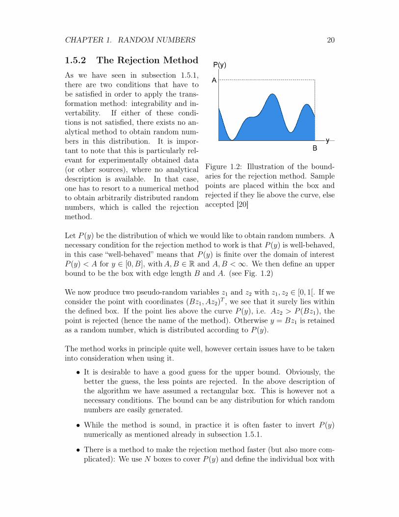
1.5.2 The Rejection Method
Figure 1.2: Illustration of the bound-aries for the rejection method. Samplepoints are placed within the box andrejected if they lie above the curve, elseaccepted [20]
As we have seen in subsection 1.5.1,there are two conditions that have tobe satisfied in order to apply the trans-formation method: integrability and in-vertability. If either of these condi-tions is not satisfied, there exists no an-alytical method to obtain random num-bers in this distribution. It is impor-tant to note that this is particularly rel-evant for experimentally obtained data(or other sources), where no analyticaldescription is available. In that case,one has to resort to a numerical methodto obtain arbitrarily distributed randomnumbers, which is called the rejectionmethod.
Let P (y) be the distribution of which we would like to obtain random numbers. Anecessary condition for the rejection method to work is that P (y) is well-behaved,in this case “well-behaved” means that P (y) is finite over the domain of interestP (y) < A for y ∈ [0, B], withA,B ∈ R and A,B <∞. We then define an upperbound to be the box with edge length B and A. (see Fig. 1.2)
We now produce two pseudo-random variables z1 and z2 with z1, z2 ∈ [0, 1[. If weconsider the point with coordinates (Bz1, Az2)T , we see that it surely lies withinthe defined box. If the point lies above the curve P (y), i.e. Az2 > P (Bz1), thepoint is rejected (hence the name of the method). Otherwise y = Bz1 is retainedas a random number, which is distributed according to P (y).
The method works in principle quite well, however certain issues have to be takeninto consideration when using it.
• It is desirable to have a good guess for the upper bound. Obviously, thebetter the guess, the less points are rejected. In the above description ofthe algorithm we have assumed a rectangular box. This is however not anecessary conditions. The bound can be any distribution for which randomnumbers are easily generated.
• While the method is sound, in practice it is often faster to invert P (y)numerically as mentioned already in subsection 1.5.1.
• There is a method to make the rejection method faster (but also more com-plicated): We use N boxes to cover P (y) and define the individual box with
CHAPTER 1. RANDOM NUMBERS 21
side length Ai and bi = Bi+1 − Bi for l ≤ i ≤ N . Then, the approximationof P (y) is much better (this is related to the idea of the Riemann-integral)
Literature
• Numerical Recipes
• D. E. Knuth: “The Art of Programming Vol. 2: Seminumerical Algorithms”(Addison-Wesley, Reading MA, 1997): Chapter 3.3.1
• J.E. Gentle, "Random number generation and Monte Carlo Methods", (Springer,Berlin, 2003).
Chapter 2
Percolation
Percolation in material science and chemistry describes the movement or filteringof fluids through porous media. The name stems originally from Latin and is stillcommon in Italian1.
A very simple and basic model of such a process was first introduced by Broadbentand Hammersley (Proc. Cambridge Phil. Soc. Vol. 53, p.629 (1957)).
While the original idea was to model the fluid motion through a porous mate-rial (e.g. a container filled with glass beads), it was found that the model hadmany other applications. Furthermore, it was observed that the model had someinteresting universal features of so called critical phenomena2.
Applications include
• General porous media: for example used in the oil industry and as a modelfor the pollution of soils
• Sol-Gel transitions
• “Mixtures” of conductors and insulators: find the point at which a conduct-ing material becomes insulating
• Spreading of fires for example in forest
• Spreading of epidemics or computer virii
• Crash of stock markets (D. Sornette, Professor at ETH)
• Landslide election victories (S. Galam)
• Recognition of antigens by T-cells (Perelson)1ita: percolare: 1 Passare attraverso. ~ filtrare. 2 Far filtrare. ( 1 pass through ~ filter, 2
make sth filter).2Critical phenomena is the collective name associated with the physics of critical points.
22
CHAPTER 2. PERCOLATION 23
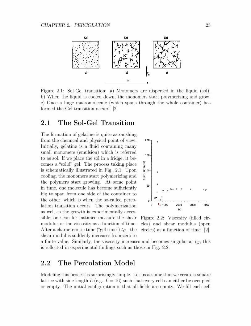
Figure 2.1: Sol-Gel transition: a) Monomers are dispersed in the liquid (sol).b) When the liquid is cooled down, the monomers start polymerizing and grow.c) Once a huge macromolecule (which spans through the whole container) hasformed the Gel transition occurs. [2]
2.1 The Sol-Gel Transition
Figure 2.2: Viscosity (filled cir-cles) and shear modulus (opencircles) as a function of time. [2]
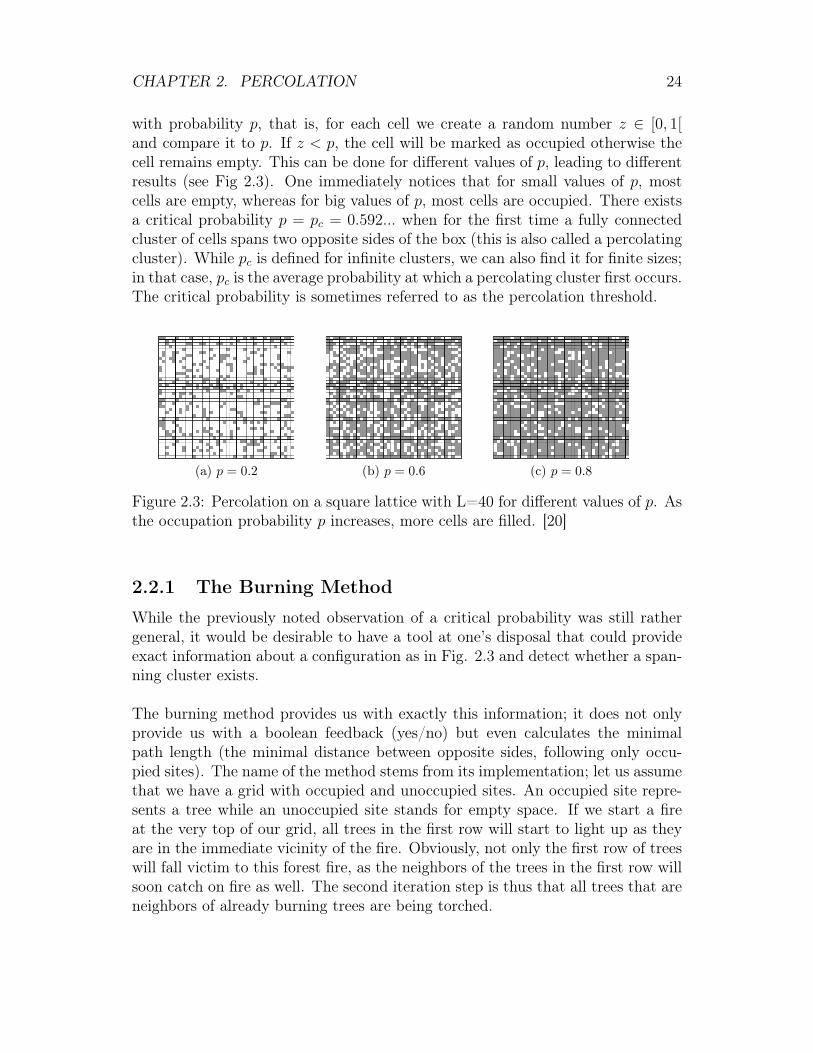
The formation of gelatine is quite astonishingfrom the chemical and physical point of view.Initially, gelatine is a fluid containing manysmall monomers (emulsion) which is referredto as sol. If we place the sol in a fridge, it be-comes a “solid” gel. The process taking placeis schematically illustrated in Fig. 2.1: Uponcooling, the monomers start polymerizing andthe polymers start growing. At some pointin time, one molecule has become sufficientlybig to span from one side of the container tothe other, which is when the so-called perco-lation transition occurs. The polymerizationas well as the growth is experimentally acces-sible; one can for instance measure the shearmodulus or the viscosity as a function of time.After a characteristic time (“gel time”) tG , theshear modulus suddenly increases from zero toa finite value. Similarly, the viscosity increases and becomes singular at tG; thisis reflected in experimental findings such as those in Fig. 2.2.
2.2 The Percolation ModelModeling this process is surprisingly simple. Let us assume that we create a squarelattice with side length L (e.g. L = 16) such that every cell can either be occupiedor empty. The initial configuration is that all fields are empty. We fill each cell
CHAPTER 2. PERCOLATION 24
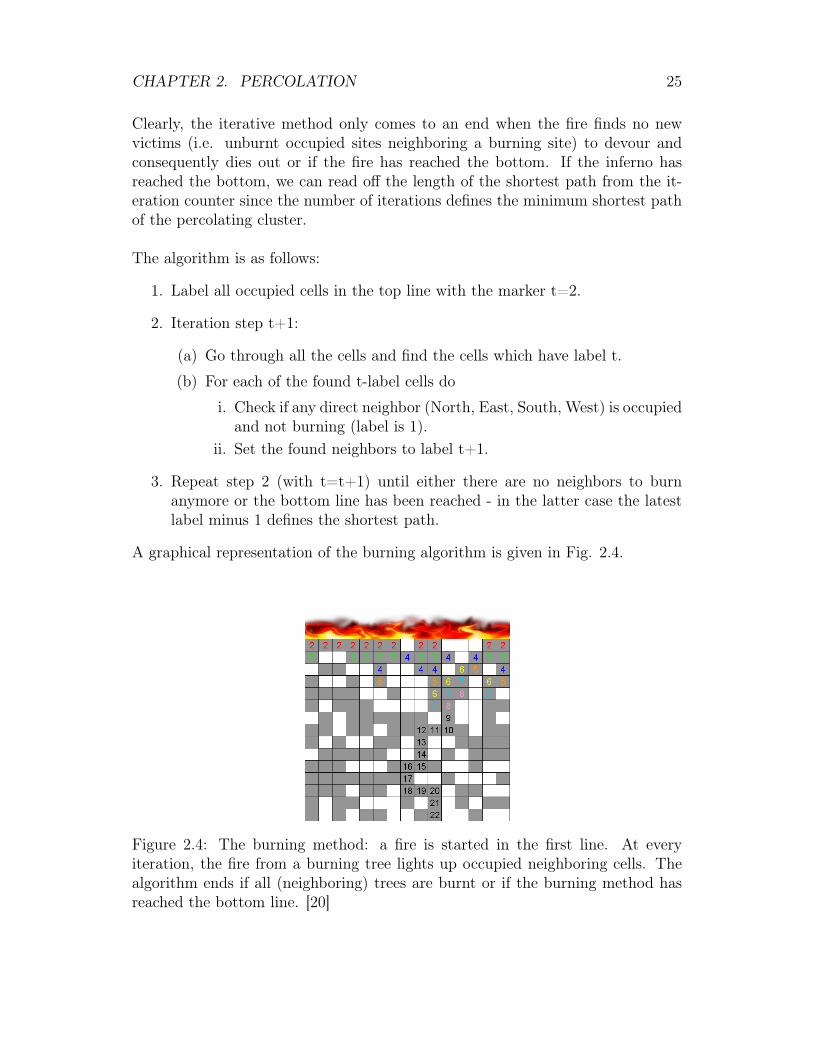
with probability p, that is, for each cell we create a random number z ∈ [0, 1[and compare it to p. If z < p, the cell will be marked as occupied otherwise thecell remains empty. This can be done for different values of p, leading to differentresults (see Fig 2.3). One immediately notices that for small values of p, mostcells are empty, whereas for big values of p, most cells are occupied. There existsa critical probability p = pc = 0.592... when for the first time a fully connectedcluster of cells spans two opposite sides of the box (this is also called a percolatingcluster). While pc is defined for infinite clusters, we can also find it for finite sizes;in that case, pc is the average probability at which a percolating cluster first occurs.The critical probability is sometimes referred to as the percolation threshold.
(a) p = 0.2 (b) p = 0.6 (c) p = 0.8
Figure 2.3: Percolation on a square lattice with L=40 for different values of p. Asthe occupation probability p increases, more cells are filled. [20]
2.2.1 The Burning Method
While the previously noted observation of a critical probability was still rathergeneral, it would be desirable to have a tool at one’s disposal that could provideexact information about a configuration as in Fig. 2.3 and detect whether a span-ning cluster exists.
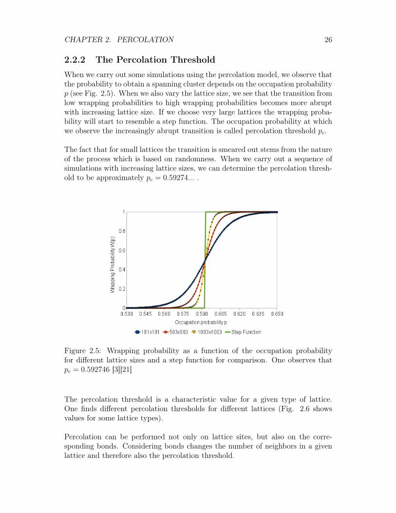
The burning method provides us with exactly this information; it does not onlyprovide us with a boolean feedback (yes/no) but even calculates the minimalpath length (the minimal distance between opposite sides, following only occu-pied sites). The name of the method stems from its implementation; let us assumethat we have a grid with occupied and unoccupied sites. An occupied site repre-sents a tree while an unoccupied site stands for empty space. If we start a fireat the very top of our grid, all trees in the first row will start to light up as theyare in the immediate vicinity of the fire. Obviously, not only the first row of treeswill fall victim to this forest fire, as the neighbors of the trees in the first row willsoon catch on fire as well. The second iteration step is thus that all trees that areneighbors of already burning trees are being torched.
CHAPTER 2. PERCOLATION 25
Clearly, the iterative method only comes to an end when the fire finds no newvictims (i.e. unburnt occupied sites neighboring a burning site) to devour andconsequently dies out or if the fire has reached the bottom. If the inferno hasreached the bottom, we can read off the length of the shortest path from the it-eration counter since the number of iterations defines the minimum shortest pathof the percolating cluster.
The algorithm is as follows:
1. Label all occupied cells in the top line with the marker t=2.
2. Iteration step t+1:
(a) Go through all the cells and find the cells which have label t.
(b) For each of the found t-label cells do
i. Check if any direct neighbor (North, East, South, West) is occupiedand not burning (label is 1).
ii. Set the found neighbors to label t+1.
3. Repeat step 2 (with t=t+1) until either there are no neighbors to burnanymore or the bottom line has been reached - in the latter case the latestlabel minus 1 defines the shortest path.
A graphical representation of the burning algorithm is given in Fig. 2.4.
Figure 2.4: The burning method: a fire is started in the first line. At everyiteration, the fire from a burning tree lights up occupied neighboring cells. Thealgorithm ends if all (neighboring) trees are burnt or if the burning method hasreached the bottom line. [20]
CHAPTER 2. PERCOLATION 26
2.2.2 The Percolation Threshold
When we carry out some simulations using the percolation model, we observe thatthe probability to obtain a spanning cluster depends on the occupation probabilityp (see Fig. 2.5). When we also vary the lattice size, we see that the transition fromlow wrapping probabilities to high wrapping probabilities becomes more abruptwith increasing lattice size. If we choose very large lattices the wrapping proba-bility will start to resemble a step function. The occupation probability at whichwe observe the increasingly abrupt transition is called percolation threshold pc.
The fact that for small lattices the transition is smeared out stems from the natureof the process which is based on randomness. When we carry out a sequence ofsimulations with increasing lattice sizes, we can determine the percolation thresh-old to be approximately pc = 0.59274... .
Figure 2.5: Wrapping probability as a function of the occupation probabilityfor different lattice sizes and a step function for comparison. One observes thatpc = 0.592746 [3][21]
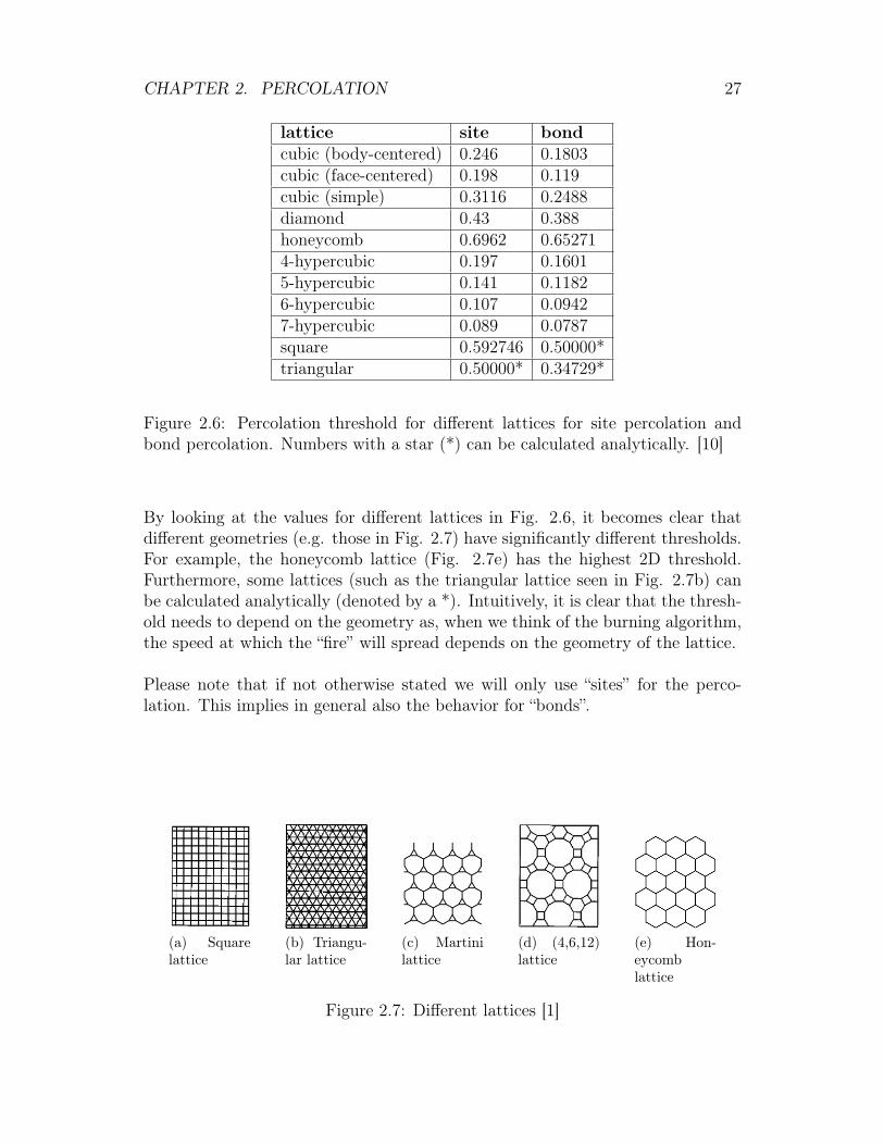
The percolation threshold is a characteristic value for a given type of lattice.One finds different percolation thresholds for different lattices (Fig. 2.6 showsvalues for some lattice types).
Percolation can be performed not only on lattice sites, but also on the corre-sponding bonds. Considering bonds changes the number of neighbors in a givenlattice and therefore also the percolation threshold.
CHAPTER 2. PERCOLATION 27
lattice site bondcubic (body-centered) 0.246 0.1803cubic (face-centered) 0.198 0.119cubic (simple) 0.3116 0.2488diamond 0.43 0.388honeycomb 0.6962 0.652714-hypercubic 0.197 0.16015-hypercubic 0.141 0.11826-hypercubic 0.107 0.09427-hypercubic 0.089 0.0787square 0.592746 0.50000*triangular 0.50000* 0.34729*
Figure 2.6: Percolation threshold for different lattices for site percolation andbond percolation. Numbers with a star (*) can be calculated analytically. [10]
By looking at the values for different lattices in Fig. 2.6, it becomes clear thatdifferent geometries (e.g. those in Fig. 2.7) have significantly different thresholds.For example, the honeycomb lattice (Fig. 2.7e) has the highest 2D threshold.Furthermore, some lattices (such as the triangular lattice seen in Fig. 2.7b) canbe calculated analytically (denoted by a *). Intuitively, it is clear that the thresh-old needs to depend on the geometry as, when we think of the burning algorithm,the speed at which the “fire” will spread depends on the geometry of the lattice.
Please note that if not otherwise stated we will only use “sites” for the perco-lation. This implies in general also the behavior for “bonds”.
(a) Squarelattice
(b) Triangu-lar lattice
(c) Martinilattice
(d) (4,6,12)lattice
(e) Hon-eycomblattice
Figure 2.7: Different lattices [1]
CHAPTER 2. PERCOLATION 28
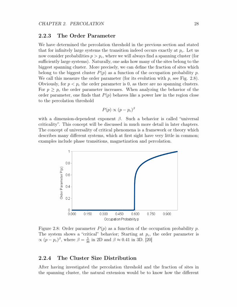
2.2.3 The Order Parameter
We have determined the percolation threshold in the previous section and statedthat for infinitely large systems the transition indeed occurs exactly at pc. Let usnow consider probabilities p > pc, where we will always find a spanning cluster (forsufficiently large systems). Naturally, one asks how many of the sites belong to thebiggest spanning cluster. More precisely, we can define the fraction of sites whichbelong to the biggest cluster P (p) as a function of the occupation probability p.We call this measure the order parameter (for its evolution with p, see Fig. 2.8).Obviously, for p < pc the order parameter is 0, as there are no spanning clusters.For p ≥ pc the order parameter increases. When analyzing the behavior of theorder parameter, one finds that P (p) behaves like a power law in the region closeto the percolation threshold
P (p) ∝ (p− pc)β
with a dimension-dependent exponent β. Such a behavior is called “universalcriticality”. This concept will be discussed in much more detail in later chapters.The concept of universality of critical phenomena is a framework or theory whichdescribes many different systems, which at first sight have very little in common;examples include phase transitions, magnetization and percolation.
Figure 2.8: Order parameter P (p) as a function of the occupation probability p.The system shows a “critical” behavior; Starting at pc, the order parameter is∝ (p− pc)β, where β = 5
36in 2D and β ≈ 0.41 in 3D. [20]
2.2.4 The Cluster Size Distribution
After having investigated the percolation threshold and the fraction of sites inthe spanning cluster, the natural extension would be to know how the different
CHAPTER 2. PERCOLATION 29
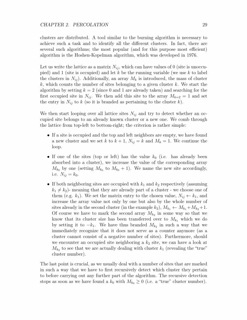
clusters are distributed. A tool similar to the burning algorithm is necessary toachieve such a task and to identify all the different clusters. In fact, there areseveral such algorithms; the most popular (and for this purpose most efficient)algorithm is the Hoshen-Kopelman algorithm, which was developed in 1976.
Let us write the lattice as a matrix Nij, which can have values of 0 (site is unoccu-pied) and 1 (site is occupied) and let k be the running variable (we use k to labelthe clusters in Nij). Additionally, an array Mk is introduced, the mass of clusterk, which counts the number of sites belonging to a given cluster k. We start thealgorithm by setting k = 2 (since 0 and 1 are already taken) and searching for thefirst occupied site in Nij. We then add this site to the array Mk=2 = 1 and setthe entry in Nij to k (so it is branded as pertaining to the cluster k).
We then start looping over all lattice sites Nij and try to detect whether an oc-cupied site belongs to an already known cluster or a new one. We comb throughthe lattice from top-left to bottom-right; the criterion is rather simple:
• If a site is occupied and the top and left neighbors are empty, we have founda new cluster and we set k to k + 1, Nij = k and Mk = 1. We continue theloop.
• If one of the sites (top or left) has the value k0 (i.e. has already beenabsorbed into a cluster), we increase the value of the corresponding arrayMk0 by one (setting Mk0 to Mk0 + 1). We name the new site accordingly,i.e. Nij = k0.
• If both neighboring sites are occupied with k1 and k2 respectively (assumingk1 6= k2)- meaning that they are already part of a cluster - we choose one ofthem (e.g. k1). We set the matrix entry to the chosen value, Nij ← k1, andincrease the array value not only by one but also by the whole number ofsites already in the second cluster (in the example k2),Mk1 ←Mk1 +Mk2 +1.Of course we have to mark the second array Mk2 in some way so that weknow that its cluster size has been transferred over to Mk1 which we doby setting it to −k1. We have thus branded Mk2 in such a way that weimmediately recognize that it does not serve as a counter anymore (as acluster cannot consist of a negative number of sites). Furthermore, shouldwe encounter an occupied site neighboring a k2 site, we can have a look atMk2 to see that we are actually dealing with cluster k1 (revealing the “true”cluster number).
The last point is crucial, as we usually deal with a number of sites that are markedin such a way that we have to first recursively detect which cluster they pertainto before carrying out any further part of the algorithm. The recursive detectionstops as soon as we have found a k0 with Mk0 ≥ 0 (i.e. a “true” cluster number).
CHAPTER 2. PERCOLATION 30
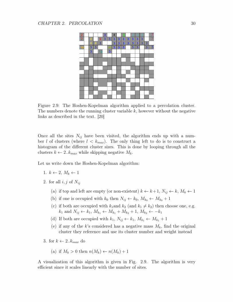
Figure 2.9: The Hoshen-Kopelman algorithm applied to a percolation cluster.The numbers denote the running cluster variable k, however without the negativelinks as described in the text. [20]
Once all the sites Nij have been visited, the algorithm ends up with a num-ber l of clusters (where l < kmax). The only thing left to do is to construct ahistogram of the different cluster sizes. This is done by looping through all theclusters k ← 2..kmax while skipping negative Mk.
Let us write down the Hoshen-Kopelman algorithm:
1. k ← 2, Mk ← 1
2. for all i, j of Nij
(a) if top and left are empty (or non-existent) k ← k+1, Nij ← k,Mk ← 1
(b) if one is occupied with k0 then Nij ← k0, Mk0 ←Mk0 + 1
(c) if both are occupied with k1and k2 (and k1 6= k2) then choose one, e.g.k1 and Nij ← k1, Mk1 ←Mk1 +Mk2 + 1, Mk2 ← −k1
(d) If both are occupied with k1, Nij ← k1, Mk1 ←Mk1 + 1
(e) if any of the k’s considered has a negative mass Mk, find the originalcluster they reference and use its cluster number and weight instead
3. for k ← 2..kmax do
(a) if Mk > 0 then n(Mk)← n(Mk) + 1
A visualization of this algorithm is given in Fig. 2.9. The algorithm is veryefficient since it scales linearly with the number of sites.
CHAPTER 2. PERCOLATION 31
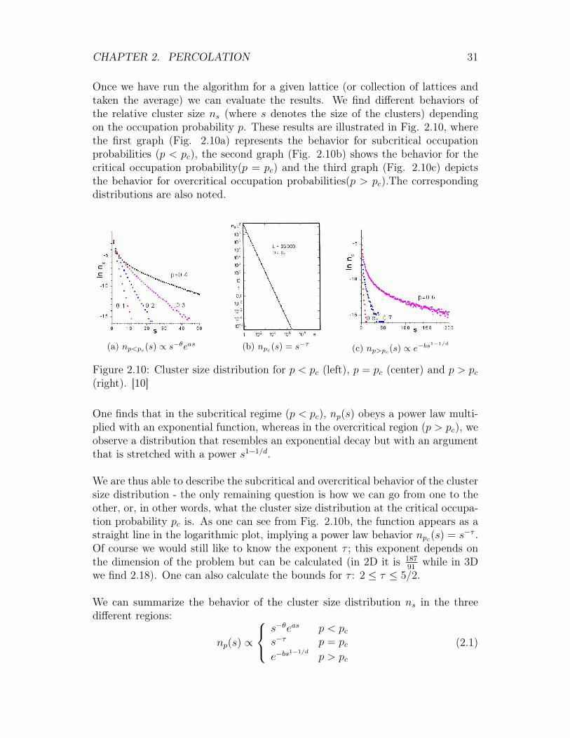
Once we have run the algorithm for a given lattice (or collection of lattices andtaken the average) we can evaluate the results. We find different behaviors ofthe relative cluster size ns (where s denotes the size of the clusters) dependingon the occupation probability p. These results are illustrated in Fig. 2.10, wherethe first graph (Fig. 2.10a) represents the behavior for subcritical occupationprobabilities (p < pc), the second graph (Fig. 2.10b) shows the behavior for thecritical occupation probability(p = pc) and the third graph (Fig. 2.10c) depictsthe behavior for overcritical occupation probabilities(p > pc).The correspondingdistributions are also noted.
(a) np<pc(s) ∝ s−θeas (b) npc(s) = s−τ (c) np>pc(s) ∝ e−bs1−1/d
Figure 2.10: Cluster size distribution for p < pc (left), p = pc (center) and p > pc(right). [10]
One finds that in the subcritical regime (p < pc), np(s) obeys a power law multi-plied with an exponential function, whereas in the overcritical region (p > pc), weobserve a distribution that resembles an exponential decay but with an argumentthat is stretched with a power s1−1/d.
We are thus able to describe the subcritical and overcritical behavior of the clustersize distribution - the only remaining question is how we can go from one to theother, or, in other words, what the cluster size distribution at the critical occupa-tion probability pc is. As one can see from Fig. 2.10b, the function appears as astraight line in the logarithmic plot, implying a power law behavior npc(s) = s−τ .Of course we would still like to know the exponent τ ; this exponent depends onthe dimension of the problem but can be calculated (in 2D it is 187
91while in 3D
we find 2.18). One can also calculate the bounds for τ : 2 ≤ τ ≤ 5/2.
We can summarize the behavior of the cluster size distribution ns in the threedifferent regions:
np(s) ∝
s−θeas p < pcs−τ p = pce−bs
1−1/dp > pc
(2.1)
CHAPTER 2. PERCOLATION 32
Figure 2.11: Scaling behavior of the percolation cluster size distribution [10]
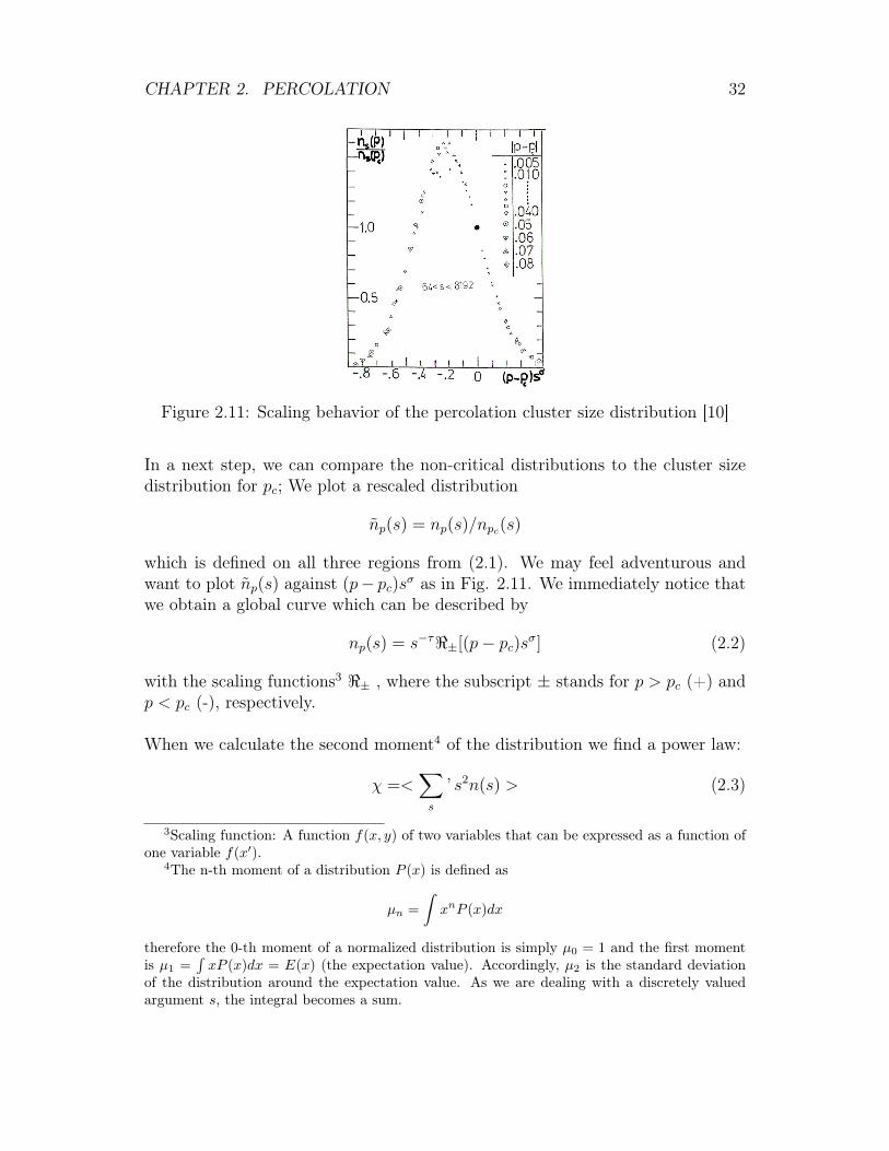
In a next step, we can compare the non-critical distributions to the cluster sizedistribution for pc; We plot a rescaled distribution
np(s) = np(s)/npc(s)
which is defined on all three regions from (2.1). We may feel adventurous andwant to plot np(s) against (p− pc)sσ as in Fig. 2.11. We immediately notice thatwe obtain a global curve which can be described by
np(s) = s−τ<±[(p− pc)sσ] (2.2)
with the scaling functions3 <± , where the subscript ± stands for p > pc (+) andp < pc (-), respectively.
When we calculate the second moment4 of the distribution we find a power law:
χ =<∑s
’ s2n(s) > (2.3)
3Scaling function: A function f(x, y) of two variables that can be expressed as a function ofone variable f(x′).
4The n-th moment of a distribution P (x) is defined as
µn =
ˆxnP (x)dx
therefore the 0-th moment of a normalized distribution is simply µ0 = 1 and the first momentis µ1 =
´xP (x)dx = E(x) (the expectation value). Accordingly, µ2 is the standard deviation
of the distribution around the expectation value. As we are dealing with a discretely valuedargument s, the integral becomes a sum.
CHAPTER 2. PERCOLATION 33
The apostrophe (’) indicates the exclusion of the largest cluster in the sum (asthe largest cluster would make χ infinite at p > pc). One finds
χ ∝ C±|p− pc|−γ (2.4)
with γ = 43/18 ≈ 2.39 in 2D and γ = 1.8 in 3D. The second moment is a verystrong indicator of pc as we can see a very clear divergence around pc. Of coursewe see a connection to the Ising model (which is explained further later on), wherethe magnetic susceptibility diverges near the critical temperature.
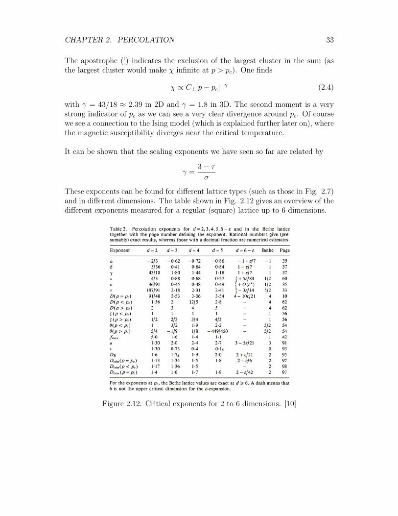
It can be shown that the scaling exponents we have seen so far are related by
γ =3− τσ
These exponents can be found for different lattice types (such as those in Fig. 2.7)and in different dimensions. The table shown in Fig. 2.12 gives an overview of thedifferent exponents measured for a regular (square) lattice up to 6 dimensions.
Figure 2.12: Critical exponents for 2 to 6 dimensions. [10]
CHAPTER 2. PERCOLATION 34
2.2.5 Size Dependence of the Order Parameter
Figure 2.13: Size depen-dence of the order parame-ter [10]
We are now going to consider the situation at thecritical occupation probability pc. The size of thelargest cluster shall be denoted by s∞ and the sidelength of the square lattice by L. When we plot s∞against L, we notice that there is a power law atwork,
s∞ ∝ Ldf
where the exponent df depends on the dimensionof the problem. For a square lattice (2D) we finddf = 91
48and for a three dimensional cube we find
df ≈ 2.51. We shall show later on that
df = d− β
ν
2.2.6 The Shortest Path
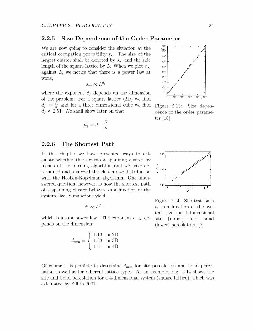
Figure 2.14: Shortest pathts as a function of the sys-tem size for 4-dimensionalsite (upper) and bond(lower) percolation. [2]
In this chapter we have presented ways to cal-culate whether there exists a spanning cluster bymeans of the burning algorithm and we have de-termined and analyzed the cluster size distributionwith the Hoshen-Kopelman algorithm. One unan-swered question, however, is how the shortest pathof a spanning cluster behaves as a function of thesystem size. Simulations yield
ts ∝ Ldmin
which is also a power law. The exponent dmin de-pends on the dimension:
dmin =
1.13 in 2D1.33 in 3D1.61 in 4D
Of course it is possible to determine dmin for site percolation and bond perco-lation as well as for different lattice types. As an example, Fig. 2.14 shows thesite and bond percolation for a 4-dimensional system (square lattice), which wascalculated by Ziff in 2001.
CHAPTER 2. PERCOLATION 35
Literature
• D. Stauffer: „Introduction to Percolation Theory“ (Taylor and Francis,1985).
• D. Stauffer and A. Aharony: „Introduction to Percolation Theory, RevisedSecond Edition“ (Taylor and Francis, 1992).
• M. Sahimi: „Applications of Percolation Theory“ (Taylor and Francis, 1994).
• G. Grimmett: „Percolation“ (Springer, 1989).
• B. Bollobas and O.Riordan: „Percolation“ (Cambridge Univ. Press, 2006).
Chapter 3
Fractals
3.1 Self-SimilarityThe fractal dimension is a concept which has been introduced in the field of fractalgeometry. The underlying idea is to find a measure to describe how well a given(fractal) object fills a certain space.
A related and simpler concept is self-similarity. Before introducing fractal di-mensions, it may therefore be useful to consider some examples of self-similarity.In a nut-shell, one could define an object to be ‘self-similar’ if it is built up ofsmaller copies of itself. Such objects occur both in mathematics and in nature.Let us consider a few examples.
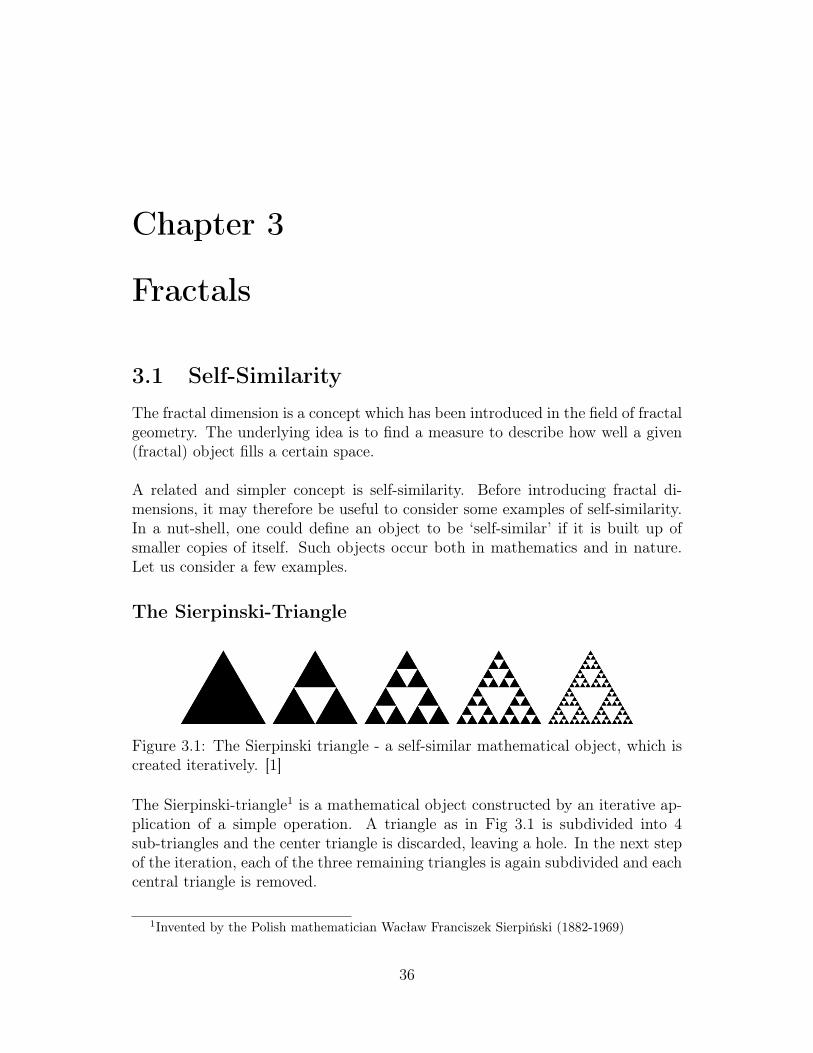
The Sierpinski-Triangle
Figure 3.1: The Sierpinski triangle - a self-similar mathematical object, which iscreated iteratively. [1]
The Sierpinski-triangle1 is a mathematical object constructed by an iterative ap-plication of a simple operation. A triangle as in Fig 3.1 is subdivided into 4sub-triangles and the center triangle is discarded, leaving a hole. In the next stepof the iteration, each of the three remaining triangles is again subdivided and eachcentral triangle is removed.
1Invented by the Polish mathematician Wacław Franciszek Sierpiński (1882-1969)
36
CHAPTER 3. FRACTALS 37
This obviously produces an object that is built up of elements that are almostthe same as the complete object, which can be referred to as ‘approximate’ self-similarity. It is only in the limit of infinite iterations that the object becomesexactly self-similar: In this case the building blocks of the object are exactly thescaled object. One also says that the object becomes a fractal in the limit ofinfinite iterations.
Self-Similarity in Nature
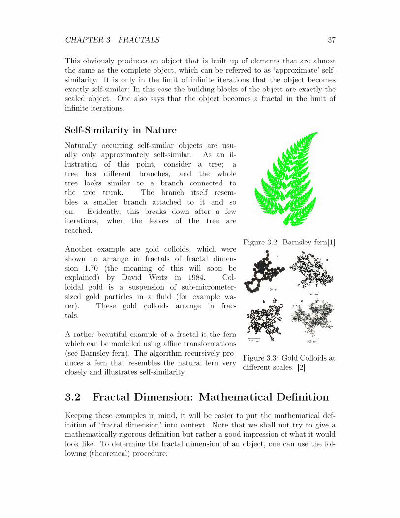
Figure 3.2: Barnsley fern[1]
Figure 3.3: Gold Colloids atdifferent scales. [2]
Naturally occurring self-similar objects are usu-ally only approximately self-similar. As an il-lustration of this point, consider a tree; atree has different branches, and the wholetree looks similar to a branch connected tothe tree trunk. The branch itself resem-bles a smaller branch attached to it and soon. Evidently, this breaks down after a fewiterations, when the leaves of the tree arereached.
Another example are gold colloids, which wereshown to arrange in fractals of fractal dimen-sion 1.70 (the meaning of this will soon beexplained) by David Weitz in 1984. Col-loidal gold is a suspension of sub-micrometer-sized gold particles in a fluid (for example wa-ter). These gold colloids arrange in frac-tals.
A rather beautiful example of a fractal is the fernwhich can be modelled using affine transformations(see Barnsley fern). The algorithm recursively pro-duces a fern that resembles the natural fern veryclosely and illustrates self-similarity.
3.2 Fractal Dimension: Mathematical DefinitionKeeping these examples in mind, it will be easier to put the mathematical def-inition of ‘fractal dimension’ into context. Note that we shall not try to give amathematically rigorous definition but rather a good impression of what it wouldlook like. To determine the fractal dimension of an object, one can use the fol-lowing (theoretical) procedure:
CHAPTER 3. FRACTALS 38
Consider all coverings of the object with spheres of radius ri ≤ ε, where ε is anarbitrary infinitesimal. Let Nε(c) be the number of spheres used in the coveringc. Then, the volume of the covering is
Vε(c) =
Nε(c)∑i=1
rdi
where d is the dimension of the spheres (i.e. the dimension of the space into whichthe object is embedded).
We define V ∗ε as the volume of the covering that uses as few spheres as possi-ble and has minimal volume
V ∗ε = minVε(c)
(minNε(c)
(Vε(c))
)The fractal dimension of the object can then be defined as
df := limε→0
log(V ∗ε /ε
d)
log (L/ε)(3.1)
Interpretation of ‘Fractal Dimensions’
The definition of the fractal dimension (3.1) can be interpreted in the followingway: When the length of the object is stretched by a factor of a, its volume(or ‘mass’) grows by a factor of adf . We obtain this interpretation by rewritingequation 3.1 (in the limit ε→ 0) as
V ∗εεd
=
(L
ε
)dfLet us consider the effect of scaling L by a. V ∗ε will scale as claimed.
As a simple example consider the Sierpinski triangle as seen in Fig. 3.4. Stretchingits sides by a factor of 2 evidently increases its volume by a factor of 3 (‘volume’in two dimensions is usually referred to as ‘area’). By inserting these valuesinto equation (3.1) we find that the Sierpinski triangle has the fractal dimensionlog(3)/ log(2) ≈ 1.585.
CHAPTER 3. FRACTALS 39
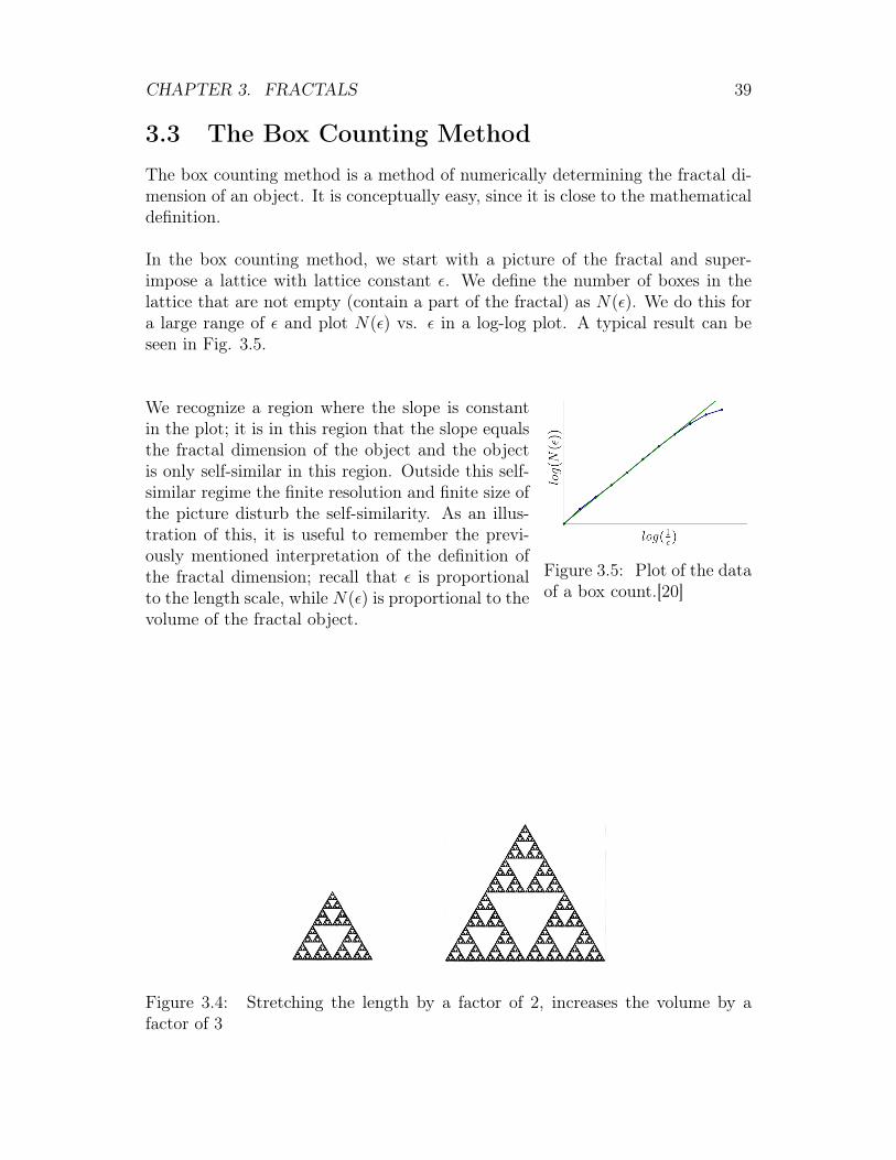
3.3 The Box Counting MethodThe box counting method is a method of numerically determining the fractal di-mension of an object. It is conceptually easy, since it is close to the mathematicaldefinition.
In the box counting method, we start with a picture of the fractal and super-impose a lattice with lattice constant ε. We define the number of boxes in thelattice that are not empty (contain a part of the fractal) as N(ε). We do this fora large range of ε and plot N(ε) vs. ε in a log-log plot. A typical result can beseen in Fig. 3.5.
Figure 3.5: Plot of the dataof a box count.[20]
We recognize a region where the slope is constantin the plot; it is in this region that the slope equalsthe fractal dimension of the object and the objectis only self-similar in this region. Outside this self-similar regime the finite resolution and finite size ofthe picture disturb the self-similarity. As an illus-tration of this, it is useful to remember the previ-ously mentioned interpretation of the definition ofthe fractal dimension; recall that ε is proportionalto the length scale, while N(ε) is proportional to thevolume of the fractal object.
Figure 3.4: Stretching the length by a factor of 2, increases the volume by afactor of 3
CHAPTER 3. FRACTALS 40
Interlude: Multifractality
By slightly adapting the box counting method, another subtlety of the fractaldimension can be understood, the so-called ‘multifractality’. Instead of only con-sidering whether a box is completely empty or not, one also counts how manyfilled dots or pixels there are in a certain box i; we will denote this number by Ni.Additionally, we introduce the fraction pi = Ni/N , where N is the total numberof occupied points. Thus pi is the fraction of dots contained in the box i.
So far we have not done anything new and original. Let us define the ‘q-mass’ Mq
of an object asMq =
∑i
pqi
Furthermore, we shall introduce the associated fractal dimension dq by the relation
Mq ∝ Ldq
where L is the length of the system.
By similar reasoning one can find
dq =1
1− qlimε→0
(limN→∞
(log((Mq/N)(1/q))
log (ε)
))For some objects dq is the same for all q and the same as the fractal dimension.For other objects, called ‘strange attractors’, one obtains different fractal dimen-sions for different values of q. This topic is of marginal interest in this course;the interested reader may find additional information by searching the keywords‘multifractality’ and ‘Renyi dimensions’.
3.4 The Sandbox Method
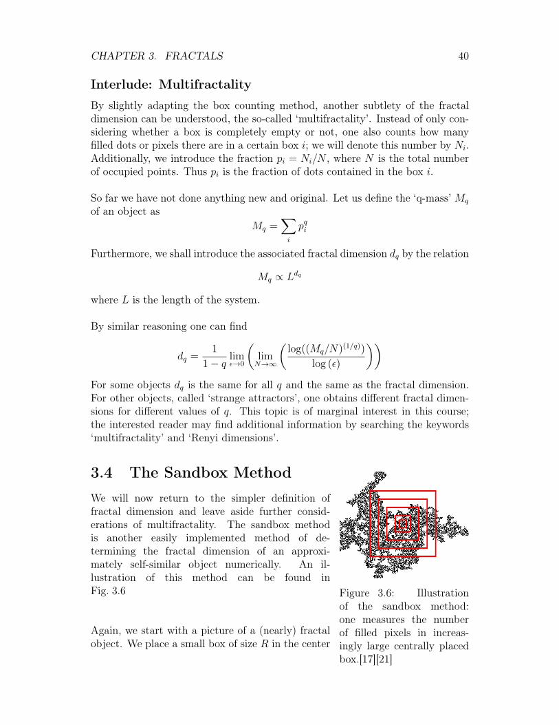
Figure 3.6: Illustrationof the sandbox method:one measures the numberof filled pixels in increas-ingly large centrally placedbox.[17][21]
We will now return to the simpler definition offractal dimension and leave aside further consid-erations of multifractality. The sandbox methodis another easily implemented method of de-termining the fractal dimension of an approxi-mately self-similar object numerically. An il-lustration of this method can be found inFig. 3.6
Again, we start with a picture of a (nearly) fractalobject. We place a small box of size R in the center
CHAPTER 3. FRACTALS 41
of the picture and count the number of occupied sites (or pixels) in the box N(R).We then successively increase the box size R in small steps until we cover thewhole picture with our box, always storing N(R). We finally plot N(R) vs. R ina log-log plot where the fractal dimension is the slope (see e.g. Fig. 3.7).
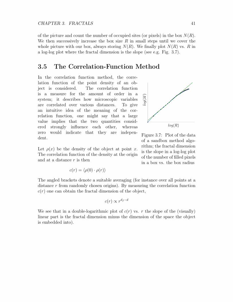
3.5 The Correlation-Function Method
Figure 3.7: Plot of the dataof a sandbox method algo-rithm; the fractal dimensionis the slope in a log-log plotof the number of filled pixelsin a box vs. the box radius
In the correlation function method, the corre-lation function of the point density of an ob-ject is considered. The correlation functionis a measure for the amount of order in asystem; it describes how microscopic variablesare correlated over various distances. To givean intuitive idea of the meaning of the cor-relation function, one might say that a largevalue implies that the two quantities consid-ered strongly influence each other, whereaszero would indicate that they are indepen-dent.
Let ρ(x) be the density of the object at point x.The correlation function of the density at the originand at a distance r is then
c(r) = 〈ρ(0) · ρ(r)〉
The angled brackets denote a suitable averaging (for instance over all points at adistance r from randomly chosen origins). By measuring the correlation functionc(r) one can obtain the fractal dimension of the object,
c(r) ∝ rdf−d
We see that in a double-logarithmic plot of c(r) vs. r the slope of the (visually)linear part is the fractal dimension minus the dimension of the space the objectis embedded into).
CHAPTER 3. FRACTALS 42
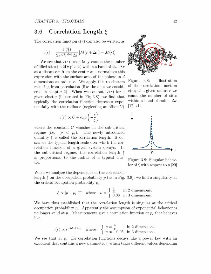
3.6 Correlation Length ξ
Figure 3.8: Illustrationof the correlation functionc(r); at a given radius r wecount the number of siteswithin a band of radius ∆r[17][21]
Figure 3.9: Singular behav-ior of ξ with respect to p [20]
The correlation function c(r) can also be written as
c(r) =Γ(d
2)
2πd/2rd−1∆r[M(r + ∆r)−M(r)]
We see that c(r) essentially counts the numberof filled sites (in 2D: pixels) within a band of size ∆rat a distance r from the center and normalizes thisexpression with the surface area of the sphere in ddimensions at radius r. We apply this to clustersresulting from percolation (like the ones we consid-ered in chapter 2). When we compute c(r) for agiven cluster (illustrated in Fig 3.8), we find thattypically the correlation function decreases expo-nentially with the radius r (neglecting an offset C)
c(r) ∝ C + exp
(−rξ
)where the constant C vanishes in the sub-criticalregime (i.e. p < pc). The newly introducedquantity ξ is called the correlation length. It de-scribes the typical length scale over which the cor-relation function of a given system decays. Inthe sub-critical regime, the correlation length ξis proportional to the radius of a typical clus-ter.
When we analyze the dependence of the correlationlength ξ on the occupation probability p (as in Fig. 3.9), we find a singularity atthe critical occupation probability pc,
ξ ∝ |p− pc|−ν where ν =
{43
in 2 dimensions;0.88 in 3 dimensions.
We have thus established that the correlation length is singular at the criticaloccupation probability pc. Apparently the assumption of exponential behavior isno longer valid at pc. Measurements give a correlation function at pc that behaveslike
c(r) ∝ r−(d−2+η) where{η = 5
24in 2 dimensions;
η ≈ −0.05 in 3 dimensions.We see that at pc, the correlation functions decays like a power law with anexponent that contains a new parameter η which takes different values depending
CHAPTER 3. FRACTALS 43
on the dimension. With this background we can move on to the most importantpart of the chapter, the finite size effects.
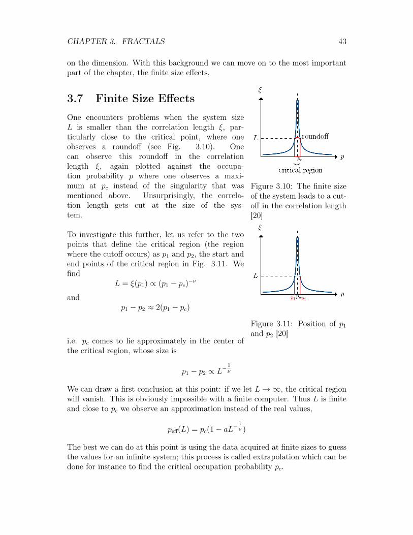
3.7 Finite Size Effects
Figure 3.10: The finite sizeof the system leads to a cut-off in the correlation length[20]
Figure 3.11: Position of p1
and p2 [20]
One encounters problems when the system sizeL is smaller than the correlation length ξ, par-ticularly close to the critical point, where oneobserves a roundoff (see Fig. 3.10). Onecan observe this roundoff in the correlationlength ξ, again plotted against the occupa-tion probability p where one observes a maxi-mum at pc instead of the singularity that wasmentioned above. Unsurprisingly, the correla-tion length gets cut at the size of the sys-tem.
To investigate this further, let us refer to the twopoints that define the critical region (the regionwhere the cutoff occurs) as p1 and p2, the start andend points of the critical region in Fig. 3.11. Wefind
L = ξ(p1) ∝ (p1 − pc)−ν
andp1 − p2 ≈ 2(p1 − pc)
i.e. pc comes to lie approximately in the center ofthe critical region, whose size is
p1 − p2 ∝ L−1ν
We can draw a first conclusion at this point: if we let L→∞, the critical regionwill vanish. This is obviously impossible with a finite computer. Thus L is finiteand close to pc we observe an approximation instead of the real values,
peff(L) = pc(1− aL−1ν )
The best we can do at this point is using the data acquired at finite sizes to guessthe values for an infinite system; this process is called extrapolation which can bedone for instance to find the critical occupation probability pc.
CHAPTER 3. FRACTALS 44
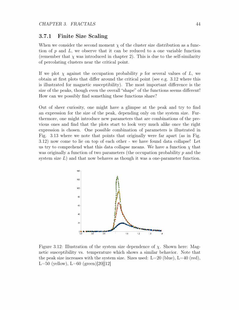
3.7.1 Finite Size Scaling
When we consider the second moment χ of the cluster size distribution as a func-tion of p and L, we observe that it can be reduced to a one variable function(remember that χ was introduced in chapter 2). This is due to the self-similarityof percolating clusters near the critical point.
If we plot χ against the occupation probability p for several values of L, weobtain at first plots that differ around the critical point (see e.g. 3.12 where thisis illustrated for magnetic susceptibility). The most important difference is thesize of the peaks, though even the overall “shape” of the functions seems different!How can we possibly find something these functions share?
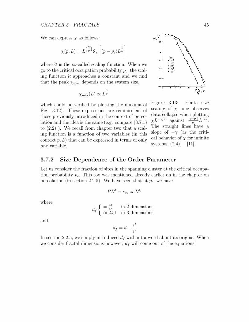
Out of sheer curiosity, one might have a glimpse at the peak and try to findan expression for the size of the peak, depending only on the system size. Fur-thermore, one might introduce new parameters that are combinations of the pre-vious ones and find that the plots start to look very much alike once the rightexpression is chosen. One possible combination of parameters is illustrated inFig. 3.13 where we note that points that originally were far apart (as in Fig.3.12) now come to lie on top of each other - we have found data collapse! Letus try to comprehend what this data collapse means. We have a function χ thatwas originally a function of two parameters (the occupation probability p and thesystem size L) and that now behaves as though it was a one-parameter function.
Figure 3.12: Illustration of the system size dependence of χ. Shown here: Mag-netic susceptibility vs. temperature which shows a similar behavior. Note thatthe peak size increases with the system size. Sizes used: L=20 (blue), L=40 (red),L=50 (yellow), L=60 (green)[20][12]
CHAPTER 3. FRACTALS 45
Figure 3.13: Finite sizescaling of χ; one observesdata collapse when plottingχL−γ/ν against |p−pc|
pcL1/ν .
The straight lines have aslope of −γ (as the criti-cal behavior of χ for infinitesystems, (2.4)) . [11]
We can express χ as follows:
χ(p, L) = L
(γν
)ℵχ[(p− pc)L
1ν
]where ℵ is the so-called scaling function. When wego to the critical occupation probability pc, the scal-ing function ℵ approaches a constant and we findthat the peak χmax depends on the system size,
χmax(L) ∝ Lγν
which could be verified by plotting the maxima ofFig. 3.12). These expressions are reminiscient ofthose previously introduced in the context of perco-lation and the idea is the same (e.g. compare (3.7.1)to (2.2) ). We recall from chapter two that a scal-ing function is a function of two variables (in thiscontext p, L) that can be expressed in terms of onlyone variable.
3.7.2 Size Dependence of the Order Parameter
Let us consider the fraction of sites in the spanning cluster at the critical occupa-tion probability pc. This too was mentioned already earlier on in the chapter onpercolation (in section 2.2.5). We have seen that at pc, we have
PLd = s∞ ∝ Ldf
wheredf
{= 91
48in 2 dimensions;
≈ 2.51 in 3 dimensions.
anddf = d− β
ν
In section 2.2.5, we simply introduced df without a word about its origins. Whenwe consider fractal dimensions however, df will come out of the equations!
CHAPTER 3. FRACTALS 46
3.8 Fractal Dimension in PercolationThe fraction of sites P in the spanning cluster (“order parameter”) is
P ∝ (p− pc)β
Futhermore, P (when considered as a function of L and p) can be written as afunction of a single parameter near pc. This is referred to as finite scaling:
P (p, L) = L−βν ℵP
[(p− pc)L
1ν
]Moreover, at pc, we find that not only the order parameter is system size depen-dent,
P ∝ L−βν
but that the number of sites is also system size dependent
M ∝ Ldf
When we combine all of this, we obtain
M ∝ PLd ∝ L
(−βν
+d
)∝ Ldf
and we have thus found the fractal dimension
df = d− β
ν
Figure 3.14: Example of avolatile fractal[2]
3.9 Examples
3.9.1 Volatile Fractals
In a volatile fractal, the cluster is “redefined” at eachscale, e.g. the path that spans L1 < L2 is not nec-essarily part of the path spanning L2 as can be seenin Fig. 3.14.
3.9.2 Bootstrap Percolation
The canonical bootstrap model is one where sites are initially occupied randomly(with a given probability p) as in the percolation model. Then, any sites that donot have at least m neighbors are removed. In the case of m = 1, all isolated sitesare removed, in the case of m = 2 all “dangling” sites are removed. This does
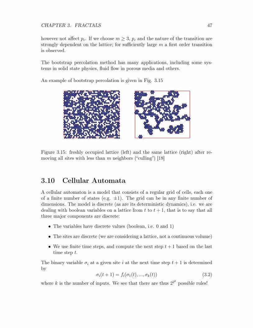
CHAPTER 3. FRACTALS 47
however not affect pc. If we choose m ≥ 3, pc and the nature of the transition arestrongly dependent on the lattice; for sufficiently large m a first order transitionis observed.
The bootstrap percolation method has many applications, including some sys-tems in solid state physics, fluid flow in porous media and others.
An example of bootstrap percolation is given in Fig. 3.15
Figure 3.15: freshly occupied lattice (left) and the same lattice (right) after re-moving all sites with less than m neighbors (“culling”) [18]
3.10 Cellular AutomataA cellular automaton is a model that consists of a regular grid of cells, each oneof a finite number of states (e.g. ±1). The grid can be in any finite number ofdimensions. The model is discrete (as are its deterministic dynamics), i.e. we aredealing with boolean variables on a lattice from t to t + 1, that is to say that allthree major components are discrete:
• The variables have discrete values (boolean, i.e. 0 and 1)
• The sites are discrete (we are considering a lattice, not a continuous volume)
• We use finite time steps, and compute the next step t+ 1 based on the lasttime step t.
The binary variable σi at a given site i at the next time step t+ 1 is determinedby
σi(t+ 1) = fi(σ1(t), ..., σk(t)) (3.2)
where k is the number of inputs. We see that there are thus 22k possible rules!
CHAPTER 3. FRACTALS 48
3.10.1 Classification of Cellular Automata
Let us consider k = 3 (3 inputs) for starters. There are 23 = 8 possible binaryentries (111, 110, 101, 100, 011, 010, 001, 000) and the rule needs to be defined foreach of these elements. Let us consider the following rule:
entries: 111 110 101 100 011 010 001 000f(n): 0 1 1 0 0 1 0 1
Furthermore, we define
c =2k−1∑n=0
2nf(n)
which for the presented rule is
c = 0 ·27 + 1 ·26 + 1 ·25 + 0 ·24 + 0 ·23 + 1 ·22 + 0 ·21 + 1 ·20 = 64 + 32 + 4 + 1 = 101
We can thus identify a rule by its c number. Let us consider a couple of rules tosee how this works (rule 4,8,20,28 and 90):
entries: 111 110 101 100 011 010 001 000f4(n): 0 0 0 0 0 1 0 0f8(n): 0 0 0 0 1 0 0 0f20(n): 0 0 0 1 0 1 0 0f28(n): 0 0 0 1 1 1 0 0f90(n): 0 1 0 1 1 0 1 0
3.10.2 Time Evolution
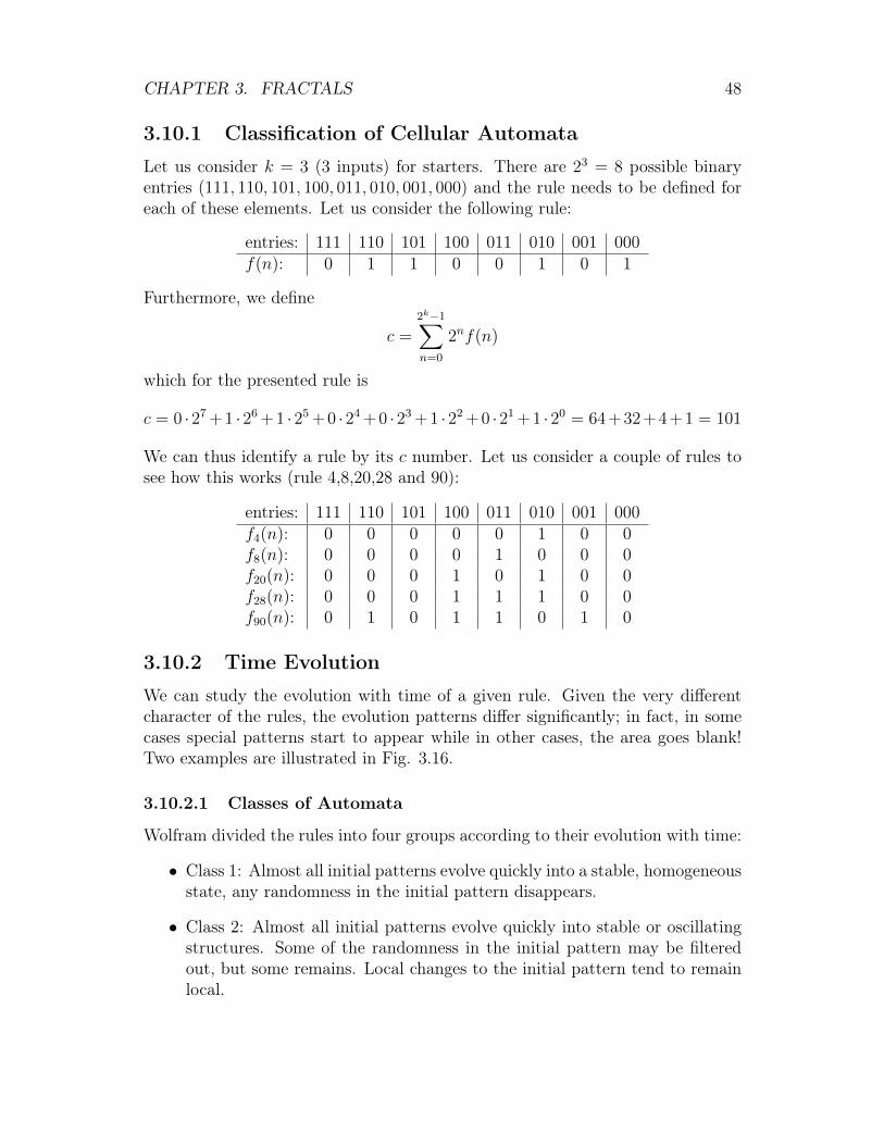
We can study the evolution with time of a given rule. Given the very differentcharacter of the rules, the evolution patterns differ significantly; in fact, in somecases special patterns start to appear while in other cases, the area goes blank!Two examples are illustrated in Fig. 3.16.
3.10.2.1 Classes of Automata
Wolfram divided the rules into four groups according to their evolution with time:
• Class 1: Almost all initial patterns evolve quickly into a stable, homogeneousstate, any randomness in the initial pattern disappears.
• Class 2: Almost all initial patterns evolve quickly into stable or oscillatingstructures. Some of the randomness in the initial pattern may be filteredout, but some remains. Local changes to the initial pattern tend to remainlocal.
CHAPTER 3. FRACTALS 49
(a) Evolution according toCA rule 126 [19]
(b) Evolution of a class 4 CA [19]
Figure 3.16: Comparison of the evolution for two completely different rules
• Class 3: Nearly all initial patterns evolve in a pseudo-random or chaoticmanner. Any stable structures that appear are quickly destroyed by thesurrounding noise. Local changes to the initial pattern tend to spread in-definitely.
• Class 4: Nearly all initial patterns evolve into structures that interact incomplex and interesting ways. Eventually a class 4 may become a class 2but the time necessary to reach that point is very large.
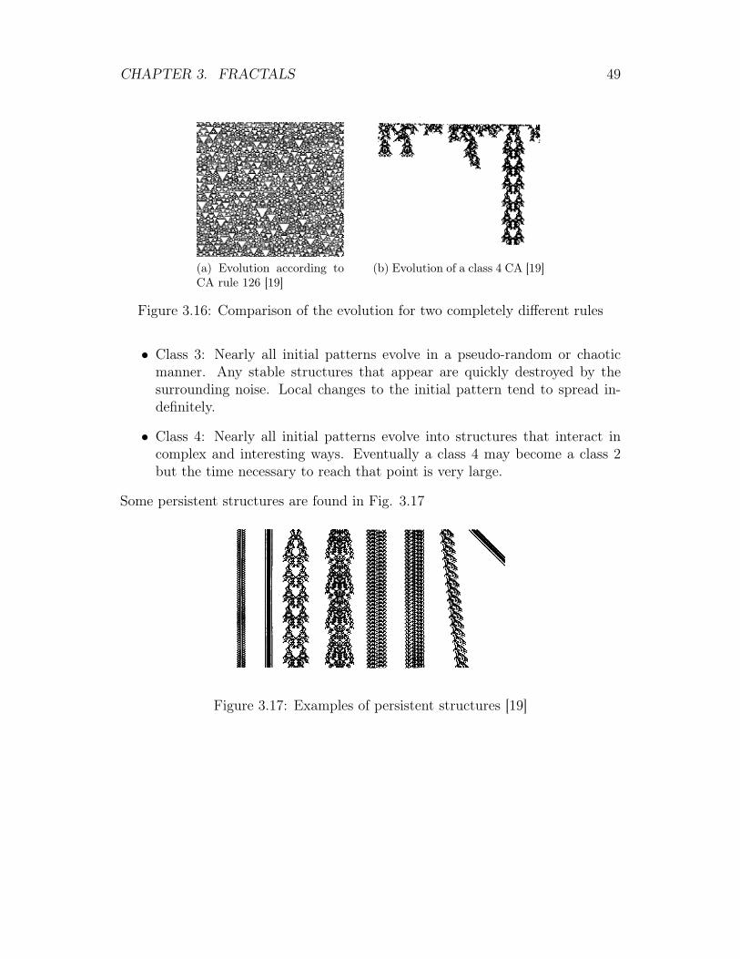
Some persistent structures are found in Fig. 3.17
Figure 3.17: Examples of persistent structures [19]
CHAPTER 3. FRACTALS 50
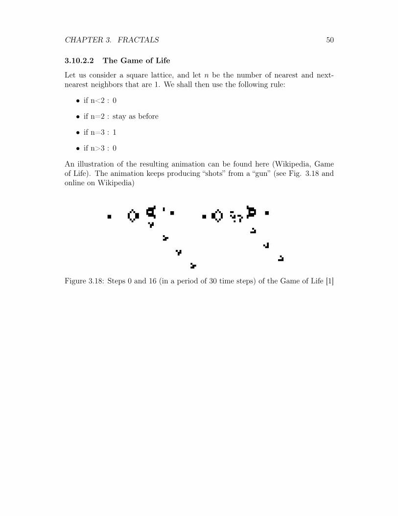
3.10.2.2 The Game of Life
Let us consider a square lattice, and let n be the number of nearest and next-nearest neighbors that are 1. We shall then use the following rule:
• if n<2 : 0
• if n=2 : stay as before
• if n=3 : 1
• if n>3 : 0
An illustration of the resulting animation can be found here (Wikipedia, Gameof Life). The animation keeps producing “shots” from a “gun” (see Fig. 3.18 andonline on Wikipedia)
Figure 3.18: Steps 0 and 16 (in a period of 30 time steps) of the Game of Life [1]
Chapter 4
Monte Carlo Methods
4.1 What is “Monte Carlo” ?The Monte Carlo methods can be characterized by their reliance on repeatedrandom sampling and averaging to obtain results. One of their major advantagesis their systematic improvement with the number of samples N , as the error ∆decreases as follows:
∆ ∝ 1√N
A good example of this is the computation of π which we shall consider in a minute.Monte Carlo methods appear frequently in the context of simulations of physicaland mathematical systems. They are also very popular when an exact solutionto a given problem cannot be found with a deterministic algorithm. They areparticularly popular in the context of higher dimensional integration (see section4.4).
4.2 Applications of Monte CarloMonte Carlo methods have a broad spectrum of applications, including the fol-lowing:
• Physics: They are used in many areas in physics, some applications includestatistical physics (e.g. Monte Carlo molecular modeling) or in QuantumChromodynamics. In the much talked about Large Hadron Collider (LHC)at CERN, Monte Carlo methods were used to simulate signals of Higgsparticles, and they are used for designing detectors (and to help understandas well as predict their behavior)
• Design: Monte Carlo methods have also penetrated areas that might - atfirst sight - seem surprising. They help in solving coupled integro-differential
51
CHAPTER 4. MONTE CARLO METHODS 52
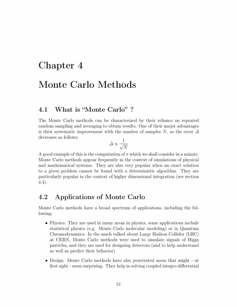
equations of radiation fields and energy transport, which is essential forglobal illumination in photorealistic images of 3D models.
• Economics: Monte Carlo models have also found their place in economicswhere they have been used e.g. for financial derivatives.
Let us consider an example that we can directly implement ourselves to becomemore familiar with this new method.
4.2.1 Computation of π
Figure 4.1: Illustration ofthe areas considered in thecomputation of π.[20]
A good illustration of this method of repeated ran-dom sampling and averaging is the computation ofthe number π.
The basic idea is rather simple: We con-sider the unit area (x ∈ [0, 1] and y ∈[0, 1]) and compare the area within the quar-ter circle, P (x, y), to the area of the unitsquare (see Fig. 4.1). This will giveπ4.
This relation is mathematically exact and can beexpressed as an integral in the following way:
π = 4
ˆ 1
0
√1− x2dx
Another way to compute π though (and learn something about Monte Carlo atthe same time) goes as follows: We consider N random points in the unit squarethat are characterized by their x and y coordinates xi, yi. Then, the number ofpoints Nc lying within the quarter circle (i.e. fulfilling the relation x2 + y2 ≤ 1)is compared to the total number N of points and the fraction will give us anapproximate value of π:
π(N) = 4Nc(N)
N
Of course, the more points we consider, the better the approximation will become.In fact, the error is ∆ = π(N) − π ∝ 1√
Nand thus really does decrease with the
number N of points. This is easy to understand. Imagine you chose just twopoints, one of which is lying inside the quarter circle, the other outside. Thiswill give you π(2) = 2, a rather atrocious approximation to 3.14159265... but ifyou pick 10 points, they will start to approximate the real value much better. For
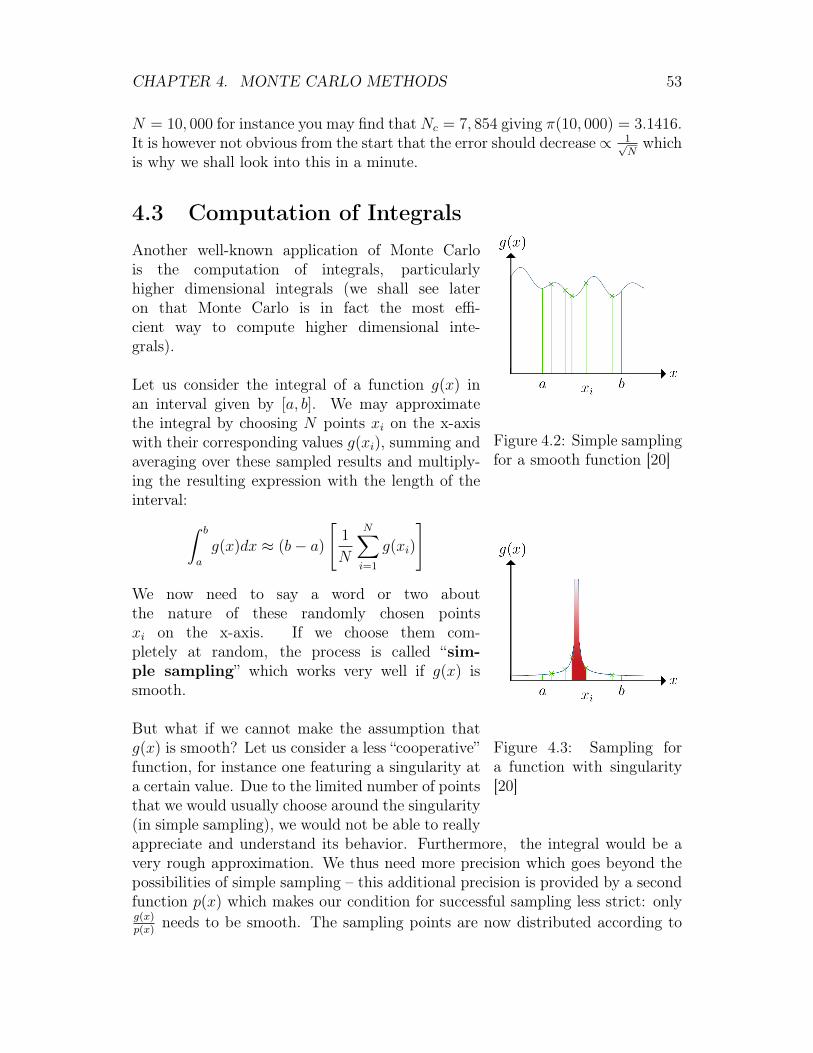
CHAPTER 4. MONTE CARLO METHODS 53
N = 10, 000 for instance you may find that Nc = 7, 854 giving π(10, 000) = 3.1416.It is however not obvious from the start that the error should decrease ∝ 1√
Nwhich
is why we shall look into this in a minute.
4.3 Computation of Integrals
Figure 4.2: Simple samplingfor a smooth function [20]
Figure 4.3: Sampling fora function with singularity[20]
Another well-known application of Monte Carlois the computation of integrals, particularlyhigher dimensional integrals (we shall see lateron that Monte Carlo is in fact the most effi-cient way to compute higher dimensional inte-grals).
Let us consider the integral of a function g(x) inan interval given by [a, b]. We may approximatethe integral by choosing N points xi on the x-axiswith their corresponding values g(xi), summing andaveraging over these sampled results and multiply-ing the resulting expression with the length of theinterval:
ˆ b
a
g(x)dx ≈ (b− a)
[1
N
N∑i=1
g(xi)
]
We now need to say a word or two aboutthe nature of these randomly chosen pointsxi on the x-axis. If we choose them com-pletely at random, the process is called “sim-ple sampling” which works very well if g(x) issmooth.
But what if we cannot make the assumption thatg(x) is smooth? Let us consider a less “cooperative”function, for instance one featuring a singularity ata certain value. Due to the limited number of pointsthat we would usually choose around the singularity(in simple sampling), we would not be able to reallyappreciate and understand its behavior. Furthermore, the integral would be avery rough approximation. We thus need more precision which goes beyond thepossibilities of simple sampling – this additional precision is provided by a secondfunction p(x) which makes our condition for successful sampling less strict: onlyg(x)p(x)
needs to be smooth. The sampling points are now distributed according to
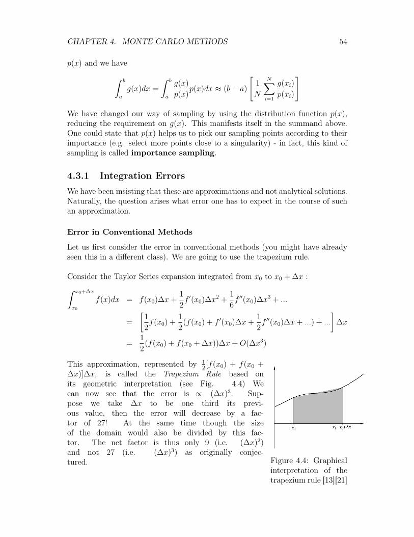
CHAPTER 4. MONTE CARLO METHODS 54
p(x) and we have
ˆ b
a
g(x)dx =
ˆ b
a
g(x)
p(x)p(x)dx ≈ (b− a)
[1
N
N∑i=1
g(xi)
p(xi)
]
We have changed our way of sampling by using the distribution function p(x),reducing the requirement on g(x). This manifests itself in the summand above.One could state that p(x) helps us to pick our sampling points according to theirimportance (e.g. select more points close to a singularity) - in fact, this kind ofsampling is called importance sampling.
4.3.1 Integration Errors
We have been insisting that these are approximations and not analytical solutions.Naturally, the question arises what error one has to expect in the course of suchan approximation.
Error in Conventional Methods
Let us first consider the error in conventional methods (you might have alreadyseen this in a different class). We are going to use the trapezium rule.
Consider the Taylor Series expansion integrated from x0 to x0 + ∆x :ˆ x0+∆x
x0
f(x)dx = f(x0)∆x+1
2f ′(x0)∆x2 +
1
6f ′′(x0)∆x3 + ...
=
[1
2f(x0) +
1
2(f(x0) + f ′(x0)∆x+
1
2f ′′(x0)∆x+ ...) + ...
]∆x
=1
2(f(x0) + f(x0 + ∆x))∆x+O(∆x3)
Figure 4.4: Graphicalinterpretation of thetrapezium rule [13][21]
This approximation, represented by 12[f(x0) + f(x0 +
∆x)]∆x, is called the Trapezium Rule based onits geometric interpretation (see Fig. 4.4) Wecan now see that the error is ∝ (∆x)3. Sup-pose we take ∆x to be one third its previ-ous value, then the error will decrease by a fac-tor of 27! At the same time though the sizeof the domain would also be divided by this fac-tor. The net factor is thus only 9 (i.e. (∆x)2)and not 27 (i.e. (∆x)3) as originally conjec-tured.
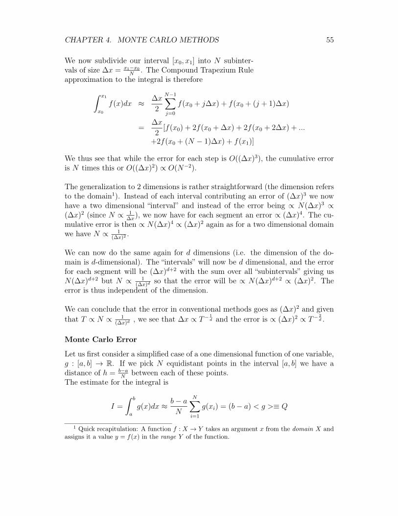
CHAPTER 4. MONTE CARLO METHODS 55
We now subdivide our interval [x0, x1] into N subinter-vals of size ∆x = x1−x0
N. The Compound Trapezium Rule
approximation to the integral is therefore
ˆ x1
x0
f(x)dx ≈ ∆x
2
N−1∑j=0
f(x0 + j∆x) + f(x0 + (j + 1)∆x)
=∆x
2[f(x0) + 2f(x0 + ∆x) + 2f(x0 + 2∆x) + ...
+2f(x0 + (N − 1)∆x) + f(x1)]
We thus see that while the error for each step is O((∆x)3), the cumulative erroris N times this or O((∆x)2) ∝ O(N−2).
The generalization to 2 dimensions is rather straightforward (the dimension refersto the domain1). Instead of each interval contributing an error of (∆x)3 we nowhave a two dimensional “interval” and instead of the error being ∝ N(∆x)3 ∝(∆x)2 (since N ∝ 1
∆x), we now have for each segment an error ∝ (∆x)4. The cu-
mulative error is then ∝ N(∆x)4 ∝ (∆x)2 again as for a two dimensional domainwe have N ∝ 1
(∆x)2 .
We can now do the same again for d dimensions (i.e. the dimension of the do-main is d-dimensional). The “intervals” will now be d dimensional, and the errorfor each segment will be (∆x)d+2 with the sum over all “subintervals” giving usN(∆x)d+2 but N ∝ 1
(∆x)dso that the error will be ∝ N(∆x)d+2 ∝ (∆x)2. The
error is thus independent of the dimension.
We can conclude that the error in conventional methods goes as (∆x)2 and giventhat T ∝ N ∝ 1
(∆x)d, we see that ∆x ∝ T−
1d and the error is ∝ (∆x)2 ∝ T−
2d .
Monte Carlo Error
Let us first consider a simplified case of a one dimensional function of one variable,g : [a, b] → R. If we pick N equidistant points in the interval [a, b] we have adistance of h = b−a
Nbetween each of these points.
The estimate for the integral is
I =
ˆ b
a
g(x)dx ≈ b− aN
N∑i=1
g(xi) = (b− a) < g >≡ Q
1 Quick recapitulation: A function f : X → Y takes an argument x from the domain X andassigns it a value y = f(x) in the range Y of the function.
CHAPTER 4. MONTE CARLO METHODS 56
where < g > stands for the sample mean of the integrand. The variance of thefunction can then be estimated using
var(g) ≡ σ2 =1
N − 1
N∑i=1
(g(xi)− < g >)2
where the denominator is N − 1 as we want to obtain the unbiased estimate ofthe variance. Using the central limit theorem, the variance of the estimate of theintegral can be estimated as
var(Q) = (b− a)2var(g)
N= (b− a)2σ
2
N
which for large N decreases like 1N. Thus, the error estimate is
δQ ≈√var(Q) = (b− a)
σ√N
We can now generalize this to multidimensional integrals:
I =
ˆ b1
a1
dx1
ˆ b2
a2
dx2...
ˆ bn
an
dxnf(x1, ..., xn)
The previous interval [a, b] becomes a hypercube V as integration volume, with
V = {x : a1 ≤ x1 ≤ b1, ...an ≤ xn ≤ bn}
so of course the formulae are adapted accordingly.Instead of the interval [a, b] appearing in the variance, we now use the hypercubeV :
var(Q) = V 2var(g)
N= V 2σ
2
Nand the error estimate becomes
δQ ≈√var(Q) = V
σ√N
but as we can see from this, the proportionality to 1√N
still remains.
Comparison of the Errors
We have seen that in conventional methods, the error of computing integrals goeswith T−
2d and thus depends on the dimension, while the error in Monte Carlo
methods is independent of the dimension. There is a crucial point at which MonteCarlo methods become more efficient,
T−2dcrit=
1√T
→ dcrit = 4 (4.1)
We can thus conclude that for d > 4, Monte Carlo becomes more efficient and istherefore used in areas where such higher dimensional integrals with d > 4 arecommonplace.
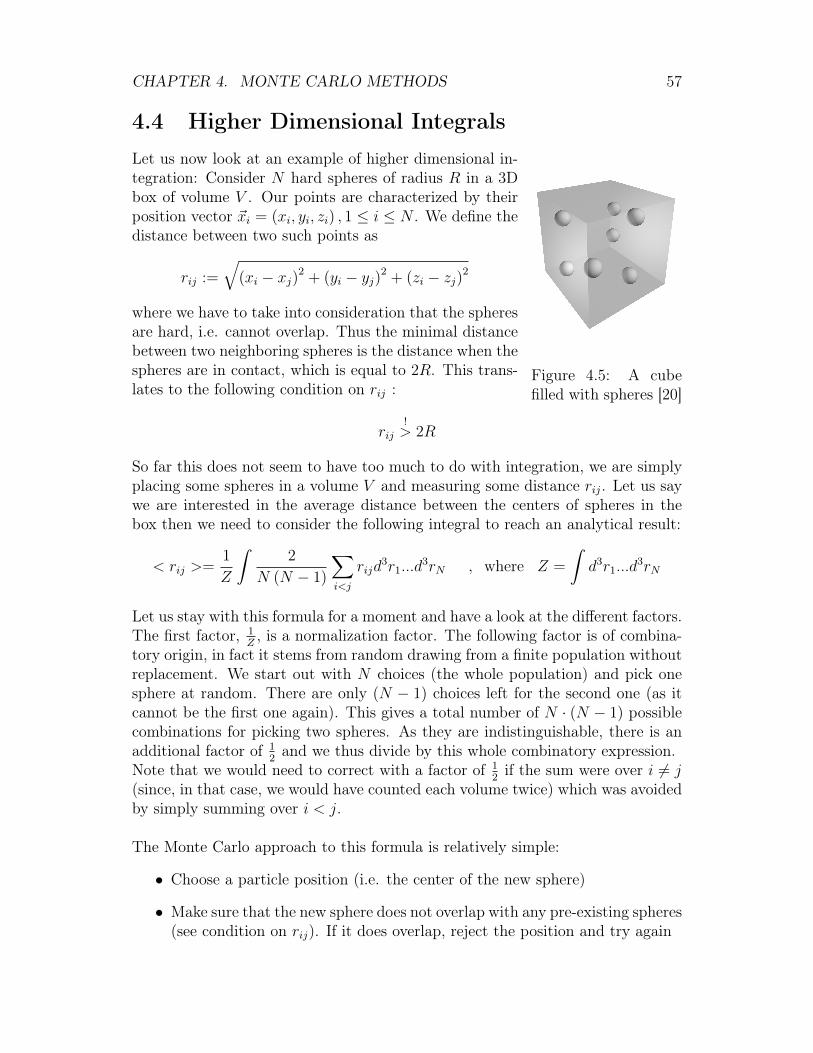
CHAPTER 4. MONTE CARLO METHODS 57
4.4 Higher Dimensional Integrals
Figure 4.5: A cubefilled with spheres [20]
Let us now look at an example of higher dimensional in-tegration: Consider N hard spheres of radius R in a 3Dbox of volume V . Our points are characterized by theirposition vector ~xi = (xi, yi, zi) , 1 ≤ i ≤ N . We define thedistance between two such points as
rij :=
√(xi − xj)2 + (yi − yj)2 + (zi − zj)2
where we have to take into consideration that the spheresare hard, i.e. cannot overlap. Thus the minimal distancebetween two neighboring spheres is the distance when thespheres are in contact, which is equal to 2R. This trans-lates to the following condition on rij :
rij!> 2R
So far this does not seem to have too much to do with integration, we are simplyplacing some spheres in a volume V and measuring some distance rij. Let us saywe are interested in the average distance between the centers of spheres in thebox then we need to consider the following integral to reach an analytical result:
< rij >=1
Z
ˆ2
N (N − 1)
∑i<j
rijd3r1...d
3rN , where Z =
ˆd3r1...d
3rN
Let us stay with this formula for a moment and have a look at the different factors.The first factor, 1
Z, is a normalization factor. The following factor is of combina-
tory origin, in fact it stems from random drawing from a finite population withoutreplacement. We start out with N choices (the whole population) and pick onesphere at random. There are only (N − 1) choices left for the second one (as itcannot be the first one again). This gives a total number of N · (N − 1) possiblecombinations for picking two spheres. As they are indistinguishable, there is anadditional factor of 1
2and we thus divide by this whole combinatory expression.
Note that we would need to correct with a factor of 12if the sum were over i 6= j
(since, in that case, we would have counted each volume twice) which was avoidedby simply summing over i < j.
The Monte Carlo approach to this formula is relatively simple:
• Choose a particle position (i.e. the center of the new sphere)
• Make sure that the new sphere does not overlap with any pre-existing spheres(see condition on rij). If it does overlap, reject the position and try again
CHAPTER 4. MONTE CARLO METHODS 58
• Once all the spheres have been placed, calculate the distances rij.
We then use these distances rij to compute the average. This procedure will con-verge and give a value that approximates the integral under the right conditions.It is important to note that our result will of course depend on the number ofspheres positioned:Imagine we had taken a ridiculously small number of spheres (let us say onlytwo!) in a rather large volume and we carried out the distance measurement.There would not be much to average over and on top of that, due to the relativeliberty of positioning the two spheres in the volume, the distance (and with it theaverage distance) would fluctuate wildly depending on the setup. If we repeatthis n times and average over it, the result will thus not converge as nicely as itwould with a relatively large number N of spheres where the space left would besmall. Placing many spheres in the volume would help the convergence but willslow down the algorithm as with more spheres comes a higher rate of rejectedpositions. For large N it is even possible that the last few spheres cannot beplaced at all! You’ll be able to analyze this in the exercises.
4.5 Canonical Monte Carlo
4.5.1 Recap: What is an Ensemble?
This section briefly explains what an ensemble is. It is a short recapitulation ofsome of the things you most likely already know from your class on thermody-namics. This section is supposed to quickly refresh your memory.
An ensemble is a set of a large number of identical systems. In the contextof physics, one usually considers the phase space (which for N particles is 6Ndimensional) of a given system. The selected points are then regarded as a col-lection of representative points in phase space. An important and ever-recurringtopic is the probability measure (on which the statistical properties depend). Letus say that we have two regions R1 and R2 with R1 having a larger measure thanR2. Consequently, if we pick a system at random from our ensemble, it is moreprobable that it is in a microstate pertaining to R1 than R2. The choice of thisprobability measure depends on the specific details of the system as well as onthe assumptions made about the ensemble.The normalizing factor of the measure is called the partition function of the en-semble. An ensemble is said to be stationary if the associated measure is time-independent. The most important ensembles are the following:
• Microcanonical ensemble: A closed system with constant number of particlesN , constant volume V and constant inner energy E
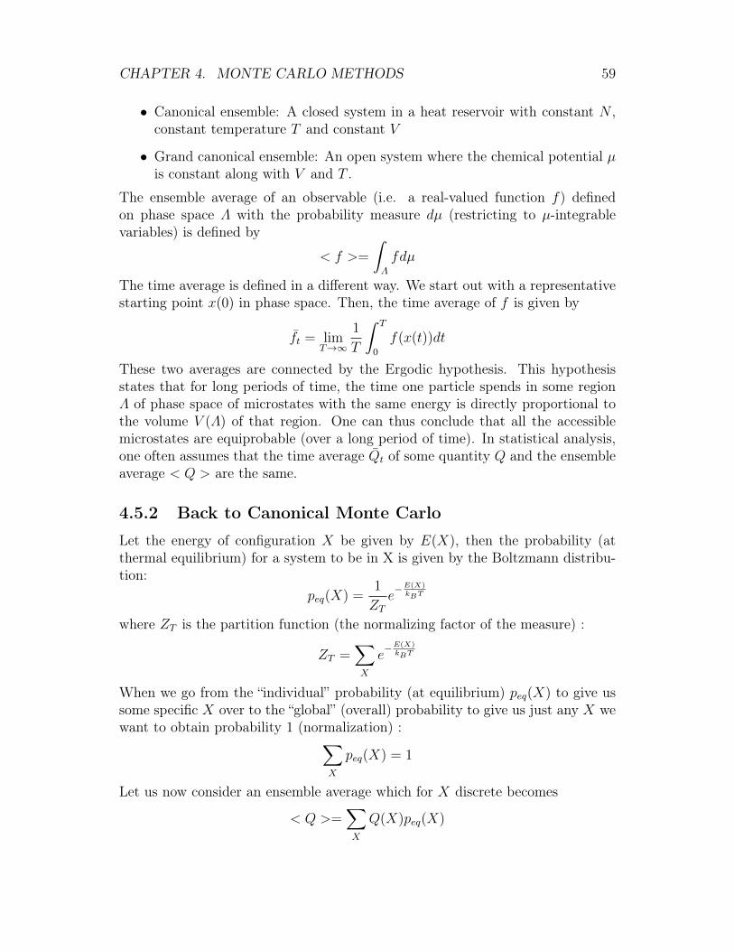
CHAPTER 4. MONTE CARLO METHODS 59
• Canonical ensemble: A closed system in a heat reservoir with constant N ,constant temperature T and constant V
• Grand canonical ensemble: An open system where the chemical potential µis constant along with V and T .
The ensemble average of an observable (i.e. a real-valued function f) definedon phase space Λ with the probability measure dµ (restricting to µ-integrablevariables) is defined by
< f >=
ˆΛ
fdµ
The time average is defined in a different way. We start out with a representativestarting point x(0) in phase space. Then, the time average of f is given by
ft = limT→∞
1
T
ˆ T
0
f(x(t))dt
These two averages are connected by the Ergodic hypothesis. This hypothesisstates that for long periods of time, the time one particle spends in some regionΛ of phase space of microstates with the same energy is directly proportional tothe volume V (Λ) of that region. One can thus conclude that all the accessiblemicrostates are equiprobable (over a long period of time). In statistical analysis,one often assumes that the time average Qt of some quantity Q and the ensembleaverage < Q > are the same.
4.5.2 Back to Canonical Monte Carlo
Let the energy of configuration X be given by E(X), then the probability (atthermal equilibrium) for a system to be in X is given by the Boltzmann distribu-tion:
peq(X) =1
ZTe−E(X)kBT
where ZT is the partition function (the normalizing factor of the measure) :
ZT =∑X
e−E(X)kBT
When we go from the “individual” probability (at equilibrium) peq(X) to give ussome specific X over to the “global” (overall) probability to give us just any X wewant to obtain probability 1 (normalization) :∑
X
peq(X) = 1
Let us now consider an ensemble average which for X discrete becomes
< Q >=∑X
Q(X)peq(X)
CHAPTER 4. MONTE CARLO METHODS 60
Figure 4.6: Energydistribution [20]
Let us say we want to calculate the ensemble average for agiven property, e.g. the energy. Unfortunately, the distri-bution of energy around the time average Et gets sharperwith increasing system size (the peak width increases withthe system size as
√Ldim while the system increases with
Ldim so the relative width decreases as 1√Ldim
).Consequently, it is inefficient to pick equally distributedconfigurations over the energy (this is similar to the sit-uation with singularities that we encountered when com-paring simple sampling to importance sampling). We arethus still (at least) one central ingredient short for thecomputation of the ensemble average.
4.5.3 M(RT )2 Algorithm
This algorithm was first described by N.C. Metropolis, A.W. Rosenbluth, M.N.Rosenbluth, A.H. Teller and E. Teller in 1953. It is a special case of a Markovchain, where the ith element Xi only depends on the previous one, Xi−1. Moreprecisely, the idea is that we carry out the previously established method of im-portance sampling through a Markov chain, going from X1 to X2 and so on, wherethe probability for a given configuration Xj is peq(Xj).
Properties of Markov Chains
As the M(RT )2 algorithm heavily relies on Markov chains, we should first lookat their properties.
We start in a given configuration X and propose a new configuration Y witha probability T (X → Y ). Again, we want the sum over all possible new configu-ration to be unity (normalization).Furthermore, the probability associated with the transition from a configurationX to a configuration Y needs to be the same as the transition probability of theinverse process, T (Y → X) (“reversibility”).Last but not least, we recall from thermodynamics the ergodic hypothesis, whichstates that thermodynamical systems are generally very “chaotic” (molecular chaos)so that all phase space volume elements corresponding to a given energy areequiprobable. More precisely, for “almost all” measurable quantities M the timeaveraged value Mt is equal to the ensemble average < M >. In the context ofMarkov chains this means that a state i is ergodic if it is aperiodic and positiverecurrent2. If all states in a Markov chain are ergodic, then the chain is called
2positive recurrent: If we start in a state i and define Ti to be the first return time to ourstate i (“hitting time”), Ti = inf{n ≥ 1 : Xn = i|X0 = i}, then the state i is recurrent if andonly if P (Ti =∞) = 0. (i.e. the hitting time is always finite). Even though the hitting time is
CHAPTER 4. MONTE CARLO METHODS 61
ergodic. Consequently, one must be able to reach any configuration X after afinite number of steps.
Let us summarize these properties:
• Ergodicity: One must be able to reach any configuration X after a finitenumber of steps.
• Normalization:∑
Y T (X → Y ) = 1
• Reversibility: T (X → Y ) = T (Y → X)
Markov Chain Probability
Now that we have established the properties of Markov chains, we want to un-derstand the second step in the process; we recall that the first one is proposinga new configuration Y . However, not every new configuration Y is also accepted.To illustrate this, let us consider the Ising model again: We may propose a newconfiguration which will increase the energy of the lattice, but depending on thetemperature it is not necessarily likely that the new configuration will also beaccepted. At low temperatures, it is unlikely that a spin flip will occur, so we’llhandle this with the acceptance probability.
Now that we have a better grasp of the concept, let us formalize these ideas:In analogy to the spin flip in the Ising model of ferromagnetism, we propose anew configuration and define an acceptance probability which will make sure thatthe model behaves the way we want. We denote the probability of acceptance ofa new configuration Y , starting from a configuration X, by A(X → Y ). In prac-tice, we might be interested a bit more in the overall probability of a configurationactually making it through these two steps; this probability is the product of thetransition probability T (X → Y ) and the acceptance probability A(X → Y ) andis called the probability of a Markov chain:
W (X → Y ) = T (X → Y ) · A(X → Y )
If we are interested in the evolution of the probability p(X, t) to find X in time,we can derive this with a logical gedankenexperiment: there are two processeschanging this probability:
• A configuration X is produced by coming from Y (this will contribute pos-itively)
• A configuration X is destroyed by going to some other configuration (thiswill decrease the probability)
finite, the state i does not need to have a finite expectation Mi = Exp [Ti]. If however the stateis positively recurrent, Mi is finite.
CHAPTER 4. MONTE CARLO METHODS 62
The first of these two is proportional to the probability for a system to be inY , p(Y ), while the second one needs to be proportional to the probability for asystem to be in X, p(X). When we combine all of this we obtain the so-calledMaster equation :
dp(X, t)
dt=∑Y
p(Y )W (Y → X)−∑Y
p(X)W (X → Y )
We can at this point conclude the properties of W (X → Y ) :Similarly to T (X → Y ), the first property is ergodicity, but it manifests itselfin a somewhat different way. Given that any configuration X must be reachableafter a finite number of steps, the transition probability T (X → Y ) cannot be zero(otherwise a state Z with T (X → Z)=0 would not be reachable) , and acceptanceis non-zero as well, so we have ∀X, Y W (X → Y ) > 0.Again, we sum over all possible “target configurations” to obtain unity, giving usthe second property (normalization).The third property, homogeneity, is new. It tells us that if we sum over all “initialconfigurations”, the product of the probability for a system to be in Y multipliedby its Markov probability for the transition to X is given by the probability for asystem to be in X. More comprehensibly, the probability for a system to be in Xis simply a result of systems coming from other configurations over to X.Quickly summarized:
• Ergodicity: ∀X, Y W (X → Y ) > 0
• Normalization:∑
Y W (X → Y ) = 1
• Homogeneity:∑
Y pst(Y )W (Y → X) = pst(X)
Note: The attentive reader might object that as W (X → Y ) = A(X → Y ) ·T (X → Y ), with both A(X → Y ) and T (X → Y ) being probabilities thathave A ≤ 1, T ≤ 1, W cannot possibly ever reach W (X → Y ) = 1. Considerthat we are looking at conditional probabilities here, as A is the probability ofacceptance for a given new configuration Y . First note that the event of choosinga new configuration t(x → y) is independent of the probability of accepting it,a(x→ y). We have that∑
Y
P (t) = 1 ,∑Y
P (a) = 1
and the conditional probability, “a provided that t” (or in plain English, theprobability to accept a new configuration produced by t), is
P (a|t) =P (a ∩ t)P (t)
=W (X → Y )
T (X → Y )
CHAPTER 4. MONTE CARLO METHODS 63
where we are now able to identify our original A(X → Y ) easily as the conditionalprobability P (a|t)!
Furthermore, for ∑i
ai = 1 ,∑i
bi = 1
we have∑ij
aibi = (a1+a2+...)(b1+b2+...)∑bi=1= a1b1+a1(1−b1)+a2b2+a2(1−b2)+... = a1+a2+... = 1
so for two independent events we get 1 again, and thus the expression is normal-izable. When we apply this to the example at hand, we find∑Y,Z
P (T (X → Y ))P (A(X → Z)) = 1
Y=Z=
∑Y
T (X → Y )A(X → Y ) =∑Y
W (X → Y )
Detailed Balance
Let us now consider a stationary state (i.e. the measure is time independent),
dp(X, t)
dt= 0
Note that all Markov processes reach a steady state. However, we want to modelthe thermal equilibrium, so we use the Boltzmann distribution,
pst(X) = peq(X)
and we obtain ∑Y
peq(Y )W (Y → X) =∑Y
peq(X)W (X → Y )
and we thus find the detailed balance condition (which is a sufficient condi-tion):
peq(Y )W (Y → X) = peq(X)W (X → Y ) (4.2)
Then, the steady state of the Markov process is the thermal equilibrium. We haveachieved this by using the Boltzmann distribution for p(X).
CHAPTER 4. MONTE CARLO METHODS 64
4.5.4 Metropolis M(RT )2
In the Metropolis algorithm, the acceptance probability A is defined as
A(X → Y ) = min(
1,peq(Y )
peq(X)
)We can now insert the Boltzmann distribution
peq(X) =1
ZTe−E(X)kBT
to findA(X → Y ) = min
(1, e−E(Y )−E(X)
kBT
)= min
(1, e− ∆EkBT
)Suppose we go to a configuration of lower energy, ∆E will be negative and wewould end up with an exponential expression like exp( |∆E|
kBT), at which point the
minimum kicks in and sets the expression to one. In other words, the acceptancewill be equal to one (“always accept“) for transitions to configurations of lowerenergy.If we go to a configuration of higher energy, ∆E will be positive and we’ll haveexp(− |∆E|
kBT) < 1 so the acceptance will increase with the temperature.
Note that a thermal equilibrium is enforced by detailed balance and we imposethat the steady state must be a Boltzmann distribution.
Glauber Dynamics
The detailed balance is a very broad condition permitting many approaches. An-other such approach was proposed by Glauber (he later obtained the Nobel prize,though not for this contribution but for his work in optics). His proposal for theacceptance probability was
AG(X → Y ) =e− ∆EkBT
1 + e− ∆EkBT
(4.3)
This also fulfills the detailed balance condition:
peq(X)W (X → Y ) = peq(Y )W (Y → X) (4.4)
Let us try to prove this.
claim: The acceptance probability (4.3) as proposed by Glauber fulfills the de-tailed balance condition (4.4).
proof:
CHAPTER 4. MONTE CARLO METHODS 65
• In a first step, let us reduce the condition (4.4) to a simpler expression. Wewrite out
W (X → Y ) = A(X → Y )T (X → Y )
to obtain
peq(X)A(X → Y )T (X → Y ) = peq(Y )A(Y → X)T (Y → X)
where we can use the reversibility (i.e. T (X → Y ) = T (Y → X)) to find
peq(X)A(X → Y ) = peq(Y )A(Y → X) (4.5)
It is thus sufficient to show that (4.3) fulfills (4.5).
• We can adapt the condition even further by recalling that (see Boltzmanndistribution)
peq(Y )
peq(X)= e
− ∆EkBT (4.6)
where the partition function ZT drops out. We can thus rewrite (4.5) bydividing both sides by peq(X) to obtain
A(X → Y ) =peq(Y )
peq(X)A(Y → X) = e
− ∆EkBT A(Y → X) (4.7)
It is thus sufficient to show that (4.3) fulfills (4.7).
• To prove that (4.3) does fulfill (4.7), we can simply write
AG(X → Y )
AG(Y → X)=
e− ∆EkBT
1 + e− ∆EkBT
·
e∆EkBT
1 + e∆EkBT
−1
= e− ∆EkBT · 1 + e
∆EkBT
e∆EkBT + 1
= e− ∆EkBT
and we have thus proven that AG does in fact fulfill the detailed balancecondition. �
The Glauber dynamics have some advantages over Metropolis once you go to lowtemperatures because of the different formulation of the acceptance.
Literature• M.H. Kalos and P.A. Whitlock: “Monte Carlo Methods” (Wiley-VCH, Berlin,
2008 )
• J.M. Hamersley and D.C. Handscomb: “Monte Carlo Methods” (Wiley andSons, N.Y., 1964)

CHAPTER 4. MONTE CARLO METHODS 66
• K. Binder and D. Heermann: “Monte Carlo Simulations in Statistical Physics”(Springer, Berlin, B li 1992)
• R.Y. Rubinstein: “Simulation and the Monte Carlo Method” (Wiley andSons, N.Y., 1981)
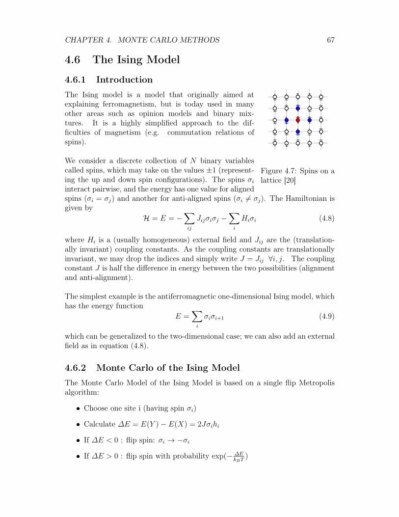
CHAPTER 4. MONTE CARLO METHODS 67
4.6 The Ising Model
4.6.1 Introduction
Figure 4.7: Spins on alattice [20]
The Ising model is a model that originally aimed atexplaining ferromagnetism, but is today used in manyother areas such as opinion models and binary mix-tures. It is a highly simplified approach to the dif-ficulties of magnetism (e.g. commutation relations ofspins).
We consider a discrete collection of N binary variablescalled spins, which may take on the values ±1 (represent-ing the up and down spin configurations). The spins σiinteract pairwise, and the energy has one value for alignedspins (σi = σj) and another for anti-aligned spins (σi 6= σj). The Hamiltonian isgiven by
H = E = −∑ij
Jijσiσj −∑i
Hiσi (4.8)
where Hi is a (usually homogeneous) external field and Jij are the (translation-ally invariant) coupling constants. As the coupling constants are translationallyinvariant, we may drop the indices and simply write J = Jij ∀i, j. The couplingconstant J is half the difference in energy between the two possibilities (alignmentand anti-alignment).
The simplest example is the antiferromagnetic one-dimensional Ising model, whichhas the energy function
E =∑i
σiσi+1 (4.9)
which can be generalized to the two-dimensional case; we can also add an externalfield as in equation (4.8).
4.6.2 Monte Carlo of the Ising Model
The Monte Carlo Model of the Ising Model is based on a single flip Metropolisalgorithm:
• Choose one site i (having spin σi)
• Calculate ∆E = E(Y )− E(X) = 2Jσihi
• If ∆E < 0 : flip spin: σi → −σi
• If ∆E > 0 : flip spin with probability exp(− ∆EkBT
)
CHAPTER 4. MONTE CARLO METHODS 68
where we have introduced hi which is the approximate local field at site i, givenby
hi =∑
nn of i
σj
The sum is characteristic of this approximation; we are only summing over thenext neighbors (nn) j of i, in this example we are thus only interested in the localfields of the next neighbors when determining hi. The notation nn for nearestneighbor is used throughout this chapter.
Note that we evaluate the acceptance probability at each step; given that theacceptance probability is very low, we need a lot of steps for something to change.We will call a group of N steps a “sweep”.
Let us consider a magnetic system; we recall the definition of the magnetic sus-ceptibility χ,
M = χH
whereM is the magnetization of the material andH is the magnetic field strength.We want to observe its evolution with the ambient temperature T . We find asingularity at the critical temperature Tc, where the magnetic susceptibility χobeys a power law with critical exponent γ:
χ ∝ (T − Tc)−γ
For finite systems we obtain a maximum instead of a singularity ( → finite sizeeffects).
A very similar formula is found for magnetization, where we define
M(T ) = limH→0〈 1
N
N∑i=1
σi〉
and find thatM ∝ |T − Tc|β
with β depending on the dimension of the model (2D: 18, 3D: ∼ 0.326).
As a side comment, note that the binary nature of this model makes it verytempting for a bitwise model (packing 64 spins together). Furthermore, moreadvanced algorithms actually do not consider locations individually but considerclusters (if you would like to know more, please visit the lecture in the springsemester).
CHAPTER 4. MONTE CARLO METHODS 69
4.6.2.1 Binary Mixtures (Lattice Gas)
A binary mixture is a mixture of two similar compounds. For instance, binaryalloys (such as copper nickel alloids) can be described with binary mixtures: Bothatoms are roughly the same size but due to energy optimization, the copper andnickel atoms try to form their own, independent clusters. We can denote Cu by+1 and Ni by −1 (in analogy to the spins from before). Unlike before, there is onenew condition that we did not need to take into consideration in the case of spins:the total number of Cu atoms and the total number of Ni atoms cannot change(while the number of e.g. up spins was free to vary) so there is an additional lawof conservation at work.
We include this in the model in the following way:
• EAA is the energy of a A-A bond
• EAB is the energy of a A-B bond
• EBB is the energy of a B-B bond
We set EAA = EBB = 0 and EAB = 1. Then, the number of each species isconstant and our conservation law is hardwired in the model since we only considerpairs of unequal particles (i.e. we can swap but not create/destroy particles).What does this mean in the Ising language? Consider the magnetization:
M(T ) = limH→0〈 1
N
N∑i=1
σi〉
and note that (due to the constant number of atoms of each species) the numberof σi = +1 and σi = −1 is constant. To see this, let us divide the indices {i} intotwo subsets:
Na := {i : 1 ≤ i ≤ N, σi = +1} , Nb := {i : 1 ≤ i ≤ N, σi = −1} (4.10)
so that
M(T ) = limH→0〈 1
N
N∑i=1
σi〉
= limH→0
1
N〈∑i∈Na
σi +∑i∈Nb
σi〉
= limH→0
1
N〈∑i∈Na
(+1) +∑i∈Nb
(−1)〉
= limH→0
1
N(|Na| − |Nb|)
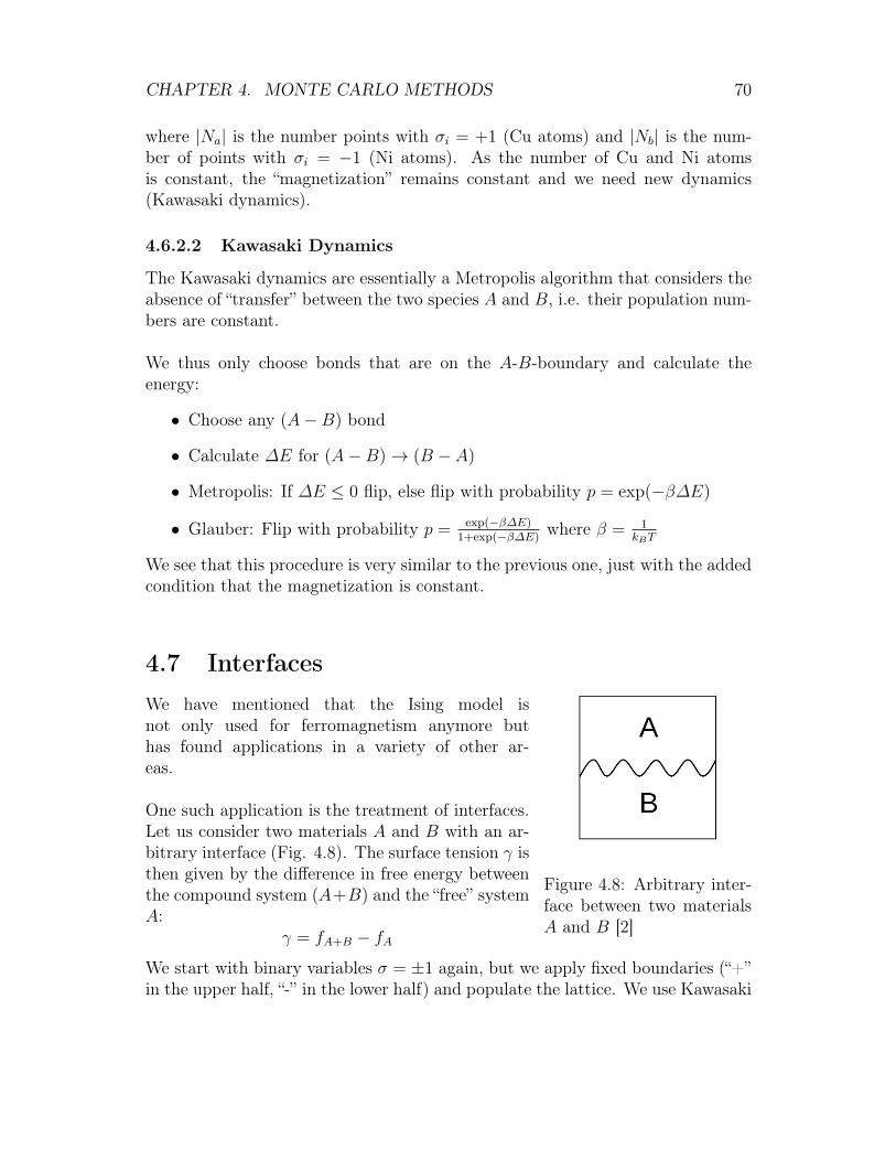
CHAPTER 4. MONTE CARLO METHODS 70
where |Na| is the number points with σi = +1 (Cu atoms) and |Nb| is the num-ber of points with σi = −1 (Ni atoms). As the number of Cu and Ni atomsis constant, the “magnetization” remains constant and we need new dynamics(Kawasaki dynamics).
4.6.2.2 Kawasaki Dynamics
The Kawasaki dynamics are essentially a Metropolis algorithm that considers theabsence of “transfer” between the two species A and B, i.e. their population num-bers are constant.
We thus only choose bonds that are on the A-B-boundary and calculate theenergy:
• Choose any (A−B) bond
• Calculate ∆E for (A−B)→ (B − A)
• Metropolis: If ∆E ≤ 0 flip, else flip with probability p = exp(−β∆E)
• Glauber: Flip with probability p = exp(−β∆E)1+exp(−β∆E)
where β = 1kBT
We see that this procedure is very similar to the previous one, just with the addedcondition that the magnetization is constant.
4.7 Interfaces
Figure 4.8: Arbitrary inter-face between two materialsA and B [2]
We have mentioned that the Ising model isnot only used for ferromagnetism anymore buthas found applications in a variety of other ar-eas.
One such application is the treatment of interfaces.Let us consider two materials A and B with an ar-bitrary interface (Fig. 4.8). The surface tension γ isthen given by the difference in free energy betweenthe compound system (A+B) and the “free” systemA:
γ = fA+B − fAWe start with binary variables σ = ±1 again, but we apply fixed boundaries (“+”in the upper half, “-” in the lower half) and populate the lattice. We use Kawasaki
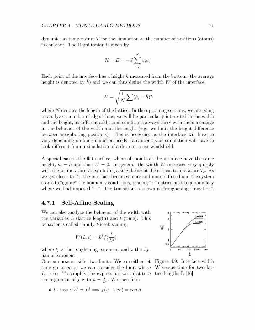
CHAPTER 4. MONTE CARLO METHODS 71
dynamics at temperature T for the simulation as the number of positions (atoms)is constant. The Hamiltonian is given by
H = E = −JN∑i,j
σiσj
Each point of the interface has a height h measured from the bottom (the averageheight is denoted by h) and we can thus define the width W of the interface:
W =
√1
N
∑i
(hi − h)2
where N denotes the length of the lattice. In the upcoming sections, we are goingto analyze a number of algorithms; we will be particularly interested in the widthand the height, as different additional conditions always carry with them a changein the behavior of the width and the height (e.g. we limit the height differencebetween neighboring positions). This is necessary as the interface will have tovary depending on our simulation needs - a cancer tissue simulation will have tolook different from a simulation of a drop on a car windshield.
A special case is the flat surface, where all points at the interface have the sameheight, hi = h and thus W = 0. In general, the width W increases very quicklywith the temperature T , exhibiting a singularity at the critical temperature Tc. Aswe get closer to Tc, the interface becomes more and more diffused and the systemstarts to “ignore” the boundary conditions, placing “+” entries next to a boundarywhere we had imposed “−”. The transition is known as “roughening transition”.
4.7.1 Self-Affine Scaling
Figure 4.9: Interface widthW versus time for two lat-tice lengths L [16]
We can also analyze the behavior of the width withthe variables L (lattice length) and t (time). Thisbehavior is called Family-Vicsek scaling
W (L, t) = Lξf(t
Lz)
where ξ is the roughening exponent and z the dy-namic exponent.One can now consider two limits: We can either lettime go to ∞ or we can consider the limit whereL → ∞. To simplify the expression, we substitutethe argument of f with u = t
Lz. We then find:
• t→∞ : W ∝ Lξ =⇒ f(u→∞) = const
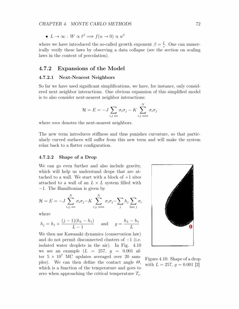
CHAPTER 4. MONTE CARLO METHODS 72
• L→∞ : W ∝ tβ =⇒ f(u→ 0) ∝ uβ
where we have introduced the so-called growth exponent β = ξz. One can numer-
ically verify these laws by observing a data collapse (see the section on scalinglaws in the context of percolation).
4.7.2 Expansions of the Model
4.7.2.1 Next-Nearest Neighbors
So far we have used significant simplifications, we have, for instance, only consid-ered next neighbor interactions. One obvious expansion of this simplified modelis to also consider next-nearest neighbor interactions:
H = E = −J∑i,j nn
σiσj −KN∑
i,j nnn
σiσj
where nnn denotes the next-nearest neighbors.
The new term introduces stiffness and thus punishes curvature, so that partic-ularly curved surfaces will suffer from this new term and will make the systemrelax back to a flatter configuration.
4.7.2.2 Shape of a Drop
Figure 4.10: Shape of a dropwith L = 257, g = 0.001 [2]
We can go even further and also include gravity,which will help us understand drops that are at-tached to a wall. We start with a block of +1 sitesattached to a wall of an L × L system filled with−1. The Hamiltonian is given by
H = E = −JN∑
i,j, nn
σiσj−KN∑
i,j, nnn
σiσj−∑j
hj∑line j
σi
where
hj = h1 +(j − 1)(hL − h1)
L− 1and g =
hL − h1
L
We then use Kawasaki dynamics (conservation law)and do not permit disconnected clusters of +1 (i.e.isolated water droplets in the air). In Fig. 4.10we see an example (L = 257, g = 0.001 af-ter 5 × 10⁷ MC updates averaged over 20 sam-ples). We can then define the contact angle Θ,which is a function of the temperature and goes tozero when approaching the critical temperature Tc.
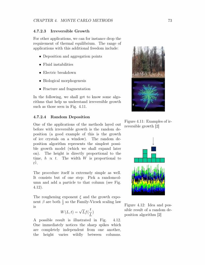
CHAPTER 4. MONTE CARLO METHODS 73
4.7.2.3 Irreversible Growth
Figure 4.11: Examples of ir-reversible growth [2]
Figure 4.12: Idea and pos-sible result of a random de-position algorithm [2]
For other applications, we can for instance drop therequirement of thermal equilibrium. The range ofapplications with this additional freedom include:
• Deposition and aggregation points
• Fluid instabilities
• Electric breakdown
• Biological morphogenesis
• Fracture and fragmentation
In the following, we shall get to know some algo-rithms that help us understand irreversible growthsuch as those seen in Fig. 4.11.
4.7.2.4 Random Deposition
One of the applications of the methods layed outbefore with irreversible growth is the random de-position (a good example of this is the growthof ice crystals on a window). The random de-position algorithm represents the simplest possi-ble growth model (which we shall expand lateron). The height is directly proportional to thetime, h ∝ t. The width W is proportional tot
12 .
The procedure itself is extremely simple as well.It consists but of one step: Pick a randomcol-umn and add a particle to that column (see Fig.4.12).
The roughening exponent ξ and the growth expo-nent β are both 1
2so the Family-Vicsek scaling law
isW (L, t) =
√Lf(
t
L)
A possible result is illustrated in Fig. 4.12.One immediately notices the sharp spikes whichare completely independent from one another,the height varies wildly between columns.
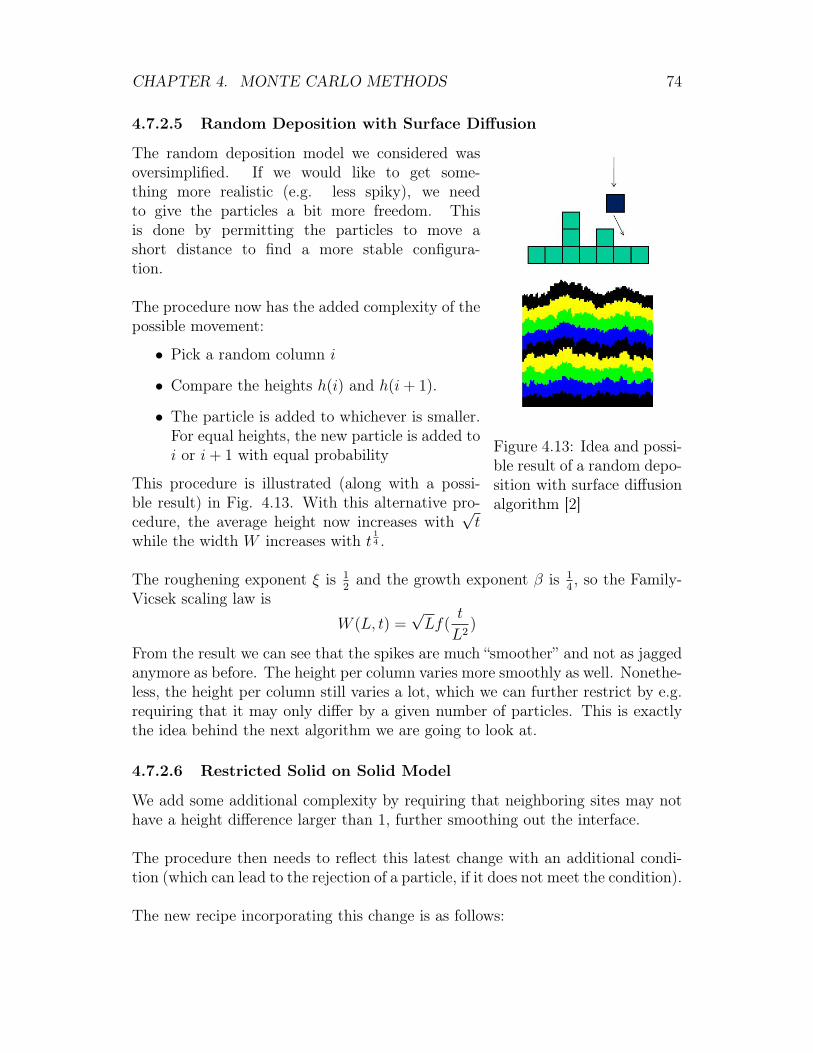
CHAPTER 4. MONTE CARLO METHODS 74
4.7.2.5 Random Deposition with Surface Diffusion
Figure 4.13: Idea and possi-ble result of a random depo-sition with surface diffusionalgorithm [2]
The random deposition model we considered wasoversimplified. If we would like to get some-thing more realistic (e.g. less spiky), we needto give the particles a bit more freedom. Thisis done by permitting the particles to move ashort distance to find a more stable configura-tion.
The procedure now has the added complexity of thepossible movement:
• Pick a random column i
• Compare the heights h(i) and h(i+ 1).
• The particle is added to whichever is smaller.For equal heights, the new particle is added toi or i+ 1 with equal probability
This procedure is illustrated (along with a possi-ble result) in Fig. 4.13. With this alternative pro-cedure, the average height now increases with
√t
while the width W increases with t14 .
The roughening exponent ξ is 12and the growth exponent β is 1
4, so the Family-
Vicsek scaling law isW (L, t) =
√Lf(
t
L2)
From the result we can see that the spikes are much “smoother” and not as jaggedanymore as before. The height per column varies more smoothly as well. Nonethe-less, the height per column still varies a lot, which we can further restrict by e.g.requiring that it may only differ by a given number of particles. This is exactlythe idea behind the next algorithm we are going to look at.
4.7.2.6 Restricted Solid on Solid Model
We add some additional complexity by requiring that neighboring sites may nothave a height difference larger than 1, further smoothing out the interface.
The procedure then needs to reflect this latest change with an additional condi-tion (which can lead to the rejection of a particle, if it does not meet the condition).
The new recipe incorporating this change is as follows:
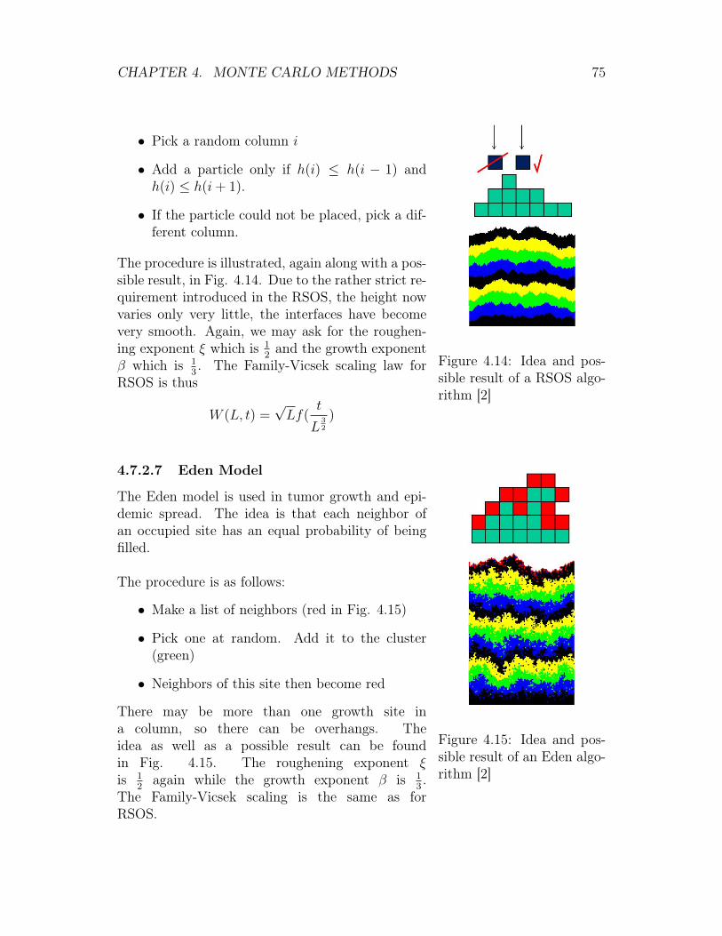
CHAPTER 4. MONTE CARLO METHODS 75
Figure 4.14: Idea and pos-sible result of a RSOS algo-rithm [2]
• Pick a random column i
• Add a particle only if h(i) ≤ h(i − 1) andh(i) ≤ h(i+ 1).
• If the particle could not be placed, pick a dif-ferent column.
The procedure is illustrated, again along with a pos-sible result, in Fig. 4.14. Due to the rather strict re-quirement introduced in the RSOS, the height nowvaries only very little, the interfaces have becomevery smooth. Again, we may ask for the roughen-ing exponent ξ which is 1
2and the growth exponent
β which is 13. The Family-Vicsek scaling law for
RSOS is thus
W (L, t) =√Lf(
t
L32
)
4.7.2.7 Eden Model
Figure 4.15: Idea and pos-sible result of an Eden algo-rithm [2]
The Eden model is used in tumor growth and epi-demic spread. The idea is that each neighbor ofan occupied site has an equal probability of beingfilled.
The procedure is as follows:
• Make a list of neighbors (red in Fig. 4.15)
• Pick one at random. Add it to the cluster(green)
• Neighbors of this site then become red
There may be more than one growth site ina column, so there can be overhangs. Theidea as well as a possible result can be foundin Fig. 4.15. The roughening exponent ξis 1
2again while the growth exponent β is 1
3.
The Family-Vicsek scaling is the same as forRSOS.
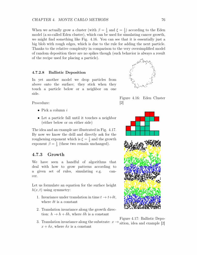
CHAPTER 4. MONTE CARLO METHODS 76
When we actually grow a cluster (with β = 13and ξ = 1
2) according to the Eden
model (a so-called Eden cluster), which can be used for simulating cancer growth,we might find something like Fig. 4.16. You can see that it is essentially just abig blob with rough edges, which is due to the rule for adding the next particle.Thanks to the relative complexity in comparison to the very oversimplified modelof random deposition there are no spikes though (such behavior is always a resultof the recipe used for placing a particle).
4.7.2.8 Ballistic Deposition
Figure 4.16: Eden Cluster[2]
Figure 4.17: Ballistic Depo-sition, idea and example [2]
In yet another model we drop particles fromabove onto the surface; they stick when theytouch a particle below or a neighbor on oneside.
Procedure:
• Pick a column i
• Let a particle fall until it touches a neighbor(either below or on either side)
The idea and an example are illustrated in Fig. 4.17.By now we know the drill and directly ask for theroughening exponent which is ξ = 1
2and the growth
exponent β = 13(these two remain unchanged).
4.7.3 Growth
We have seen a handful of algorithms thatdeal with how to grow patterns according toa given set of rules, simulating e.g. can-cer.
Let us formulate an equation for the surface heighth(x, t) using symmetry:
1. Invariance under translation in time t→ t+δt,where δt is a constant
2. Translation invariance along the growth direc-tion: h→ h+ δh, where δh is a constant
3. Translation invariance along the substrate: x→x+ δx, where δx is a constant
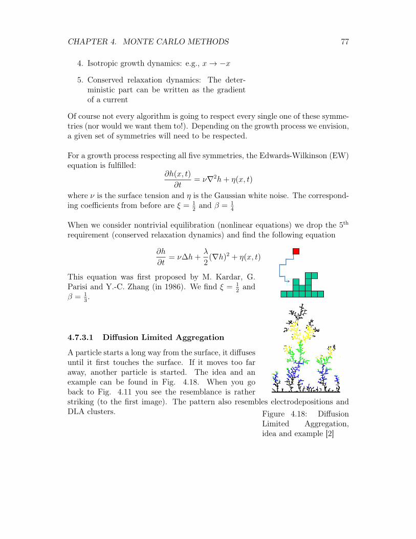
CHAPTER 4. MONTE CARLO METHODS 77
4. Isotropic growth dynamics: e.g., x→ −x
5. Conserved relaxation dynamics: The deter-ministic part can be written as the gradientof a current
Of course not every algorithm is going to respect every single one of these symme-tries (nor would we want them to!). Depending on the growth process we envision,a given set of symmetries will need to be respected.
For a growth process respecting all five symmetries, the Edwards-Wilkinson (EW)equation is fulfilled:
∂h(x, t)
∂t= ν∇2h+ η(x, t)
where ν is the surface tension and η is the Gaussian white noise. The correspond-ing coefficients from before are ξ = 1
2and β = 1
4
When we consider nontrivial equilibration (nonlinear equations) we drop the 5th
requirement (conserved relaxation dynamics) and find the following equation
∂h
∂t= ν∆h+
λ
2(∇h)2 + η(x, t)
Figure 4.18: DiffusionLimited Aggregation,idea and example [2]
This equation was first proposed by M. Kardar, G.Parisi and Y.-C. Zhang (in 1986). We find ξ = 1
2and
β = 13.
4.7.3.1 Diffusion Limited Aggregation
A particle starts a long way from the surface, it diffusesuntil it first touches the surface. If it moves too faraway, another particle is started. The idea and anexample can be found in Fig. 4.18. When you goback to Fig. 4.11 you see the resemblance is ratherstriking (to the first image). The pattern also resembles electrodepositions andDLA clusters.
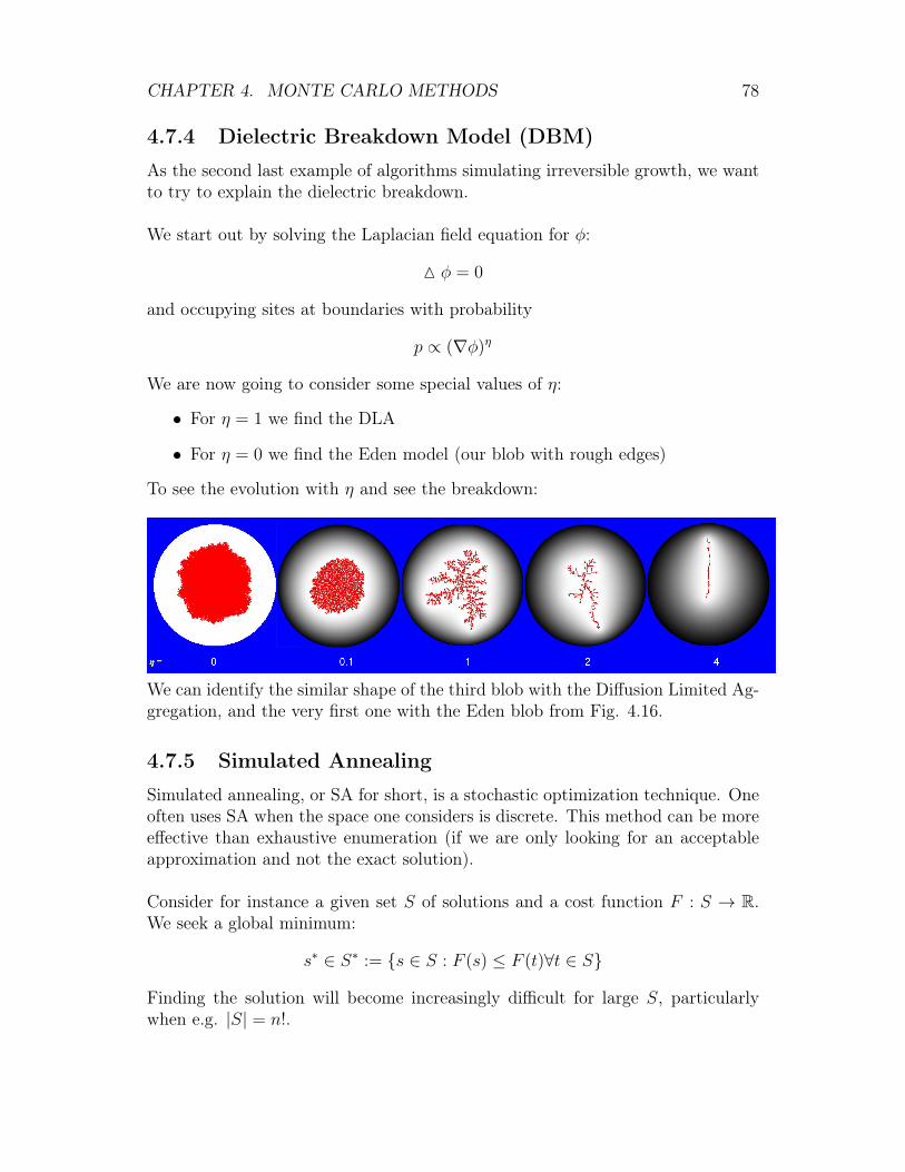
CHAPTER 4. MONTE CARLO METHODS 78
4.7.4 Dielectric Breakdown Model (DBM)
As the second last example of algorithms simulating irreversible growth, we wantto try to explain the dielectric breakdown.
We start out by solving the Laplacian field equation for φ:
M φ = 0
and occupying sites at boundaries with probability
p ∝ (∇φ)η
We are now going to consider some special values of η:
• For η = 1 we find the DLA
• For η = 0 we find the Eden model (our blob with rough edges)
To see the evolution with η and see the breakdown:
We can identify the similar shape of the third blob with the Diffusion Limited Ag-gregation, and the very first one with the Eden blob from Fig. 4.16.
4.7.5 Simulated Annealing
Simulated annealing, or SA for short, is a stochastic optimization technique. Oneoften uses SA when the space one considers is discrete. This method can be moreeffective than exhaustive enumeration (if we are only looking for an acceptableapproximation and not the exact solution).
Consider for instance a given set S of solutions and a cost function F : S → R.We seek a global minimum:
s∗ ∈ S∗ := {s ∈ S : F (s) ≤ F (t)∀t ∈ S}
Finding the solution will become increasingly difficult for large S, particularlywhen e.g. |S| = n!.
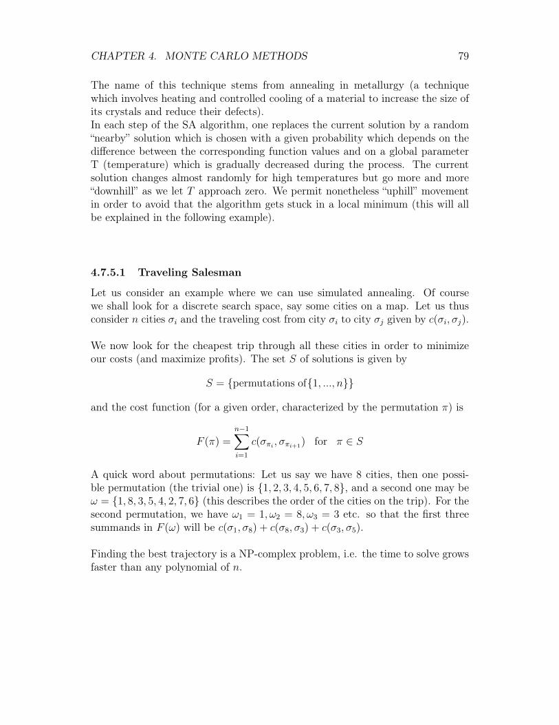
CHAPTER 4. MONTE CARLO METHODS 79
The name of this technique stems from annealing in metallurgy (a techniquewhich involves heating and controlled cooling of a material to increase the size ofits crystals and reduce their defects).In each step of the SA algorithm, one replaces the current solution by a random“nearby” solution which is chosen with a given probability which depends on thedifference between the corresponding function values and on a global parameterT (temperature) which is gradually decreased during the process. The currentsolution changes almost randomly for high temperatures but go more and more“downhill” as we let T approach zero. We permit nonetheless “uphill” movementin order to avoid that the algorithm gets stuck in a local minimum (this will allbe explained in the following example).
4.7.5.1 Traveling Salesman
Let us consider an example where we can use simulated annealing. Of coursewe shall look for a discrete search space, say some cities on a map. Let us thusconsider n cities σi and the traveling cost from city σi to city σj given by c(σi, σj).
We now look for the cheapest trip through all these cities in order to minimizeour costs (and maximize profits). The set S of solutions is given by
S = {permutations of{1, ..., n}}
and the cost function (for a given order, characterized by the permutation π) is
F (π) =n−1∑i=1
c(σπi , σπi+1) for π ∈ S
A quick word about permutations: Let us say we have 8 cities, then one possi-ble permutation (the trivial one) is {1, 2, 3, 4, 5, 6, 7, 8}, and a second one may beω = {1, 8, 3, 5, 4, 2, 7, 6} (this describes the order of the cities on the trip). For thesecond permutation, we have ω1 = 1, ω2 = 8, ω3 = 3 etc. so that the first threesummands in F (ω) will be c(σ1, σ8) + c(σ8, σ3) + c(σ3, σ5).
Finding the best trajectory is a NP-complex problem, i.e. the time to solve growsfaster than any polynomial of n.
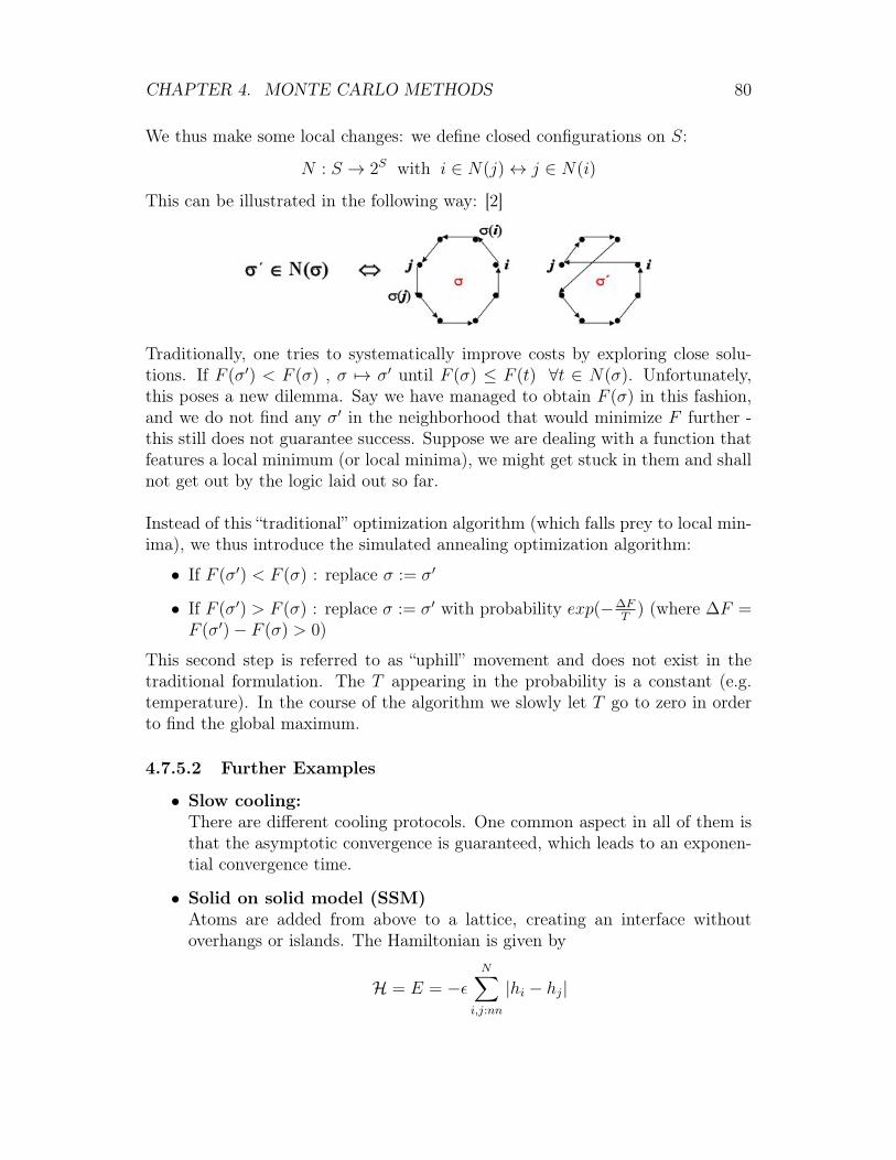
CHAPTER 4. MONTE CARLO METHODS 80
We thus make some local changes: we define closed configurations on S:
N : S → 2S with i ∈ N(j)↔ j ∈ N(i)
This can be illustrated in the following way: [2]
Traditionally, one tries to systematically improve costs by exploring close solu-tions. If F (σ′) < F (σ) , σ 7→ σ′ until F (σ) ≤ F (t) ∀t ∈ N(σ). Unfortunately,this poses a new dilemma. Say we have managed to obtain F (σ) in this fashion,and we do not find any σ′ in the neighborhood that would minimize F further -this still does not guarantee success. Suppose we are dealing with a function thatfeatures a local minimum (or local minima), we might get stuck in them and shallnot get out by the logic laid out so far.
Instead of this “traditional” optimization algorithm (which falls prey to local min-ima), we thus introduce the simulated annealing optimization algorithm:
• If F (σ′) < F (σ) : replace σ := σ′
• If F (σ′) > F (σ) : replace σ := σ′ with probability exp(−∆FT
) (where ∆F =F (σ′)− F (σ) > 0)
This second step is referred to as “uphill” movement and does not exist in thetraditional formulation. The T appearing in the probability is a constant (e.g.temperature). In the course of the algorithm we slowly let T go to zero in orderto find the global maximum.
4.7.5.2 Further Examples
• Slow cooling:There are different cooling protocols. One common aspect in all of them isthat the asymptotic convergence is guaranteed, which leads to an exponen-tial convergence time.
• Solid on solid model (SSM)Atoms are added from above to a lattice, creating an interface withoutoverhangs or islands. The Hamiltonian is given by
H = E = −εN∑
i,j:nn
|hi − hj|
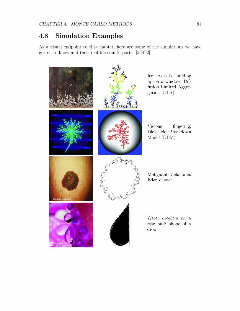
CHAPTER 4. MONTE CARLO METHODS 81
4.8 Simulation ExamplesAs a visual endpoint to this chapter, here are some of the simulations we havegotten to know and their real life counterparts: [5][4][2]

CHAPTER 4. MONTE CARLO METHODS 82
Literature• M.H. Kalos and P.A. Whitlock: “Monte Carlo Methods” (Wiley-VCH, Berlin,
2008 )
• J.M. Hamersley and D.C. Handscomb: “Monte Carlo Methods” (Wiley andSons, N.Y., 1964)
• K. Binder and D. Heermann: “Monte Carlo Simulations in Statistical Physics”(Springer, Berlin, B li 1992)
• R.Y. Rubinstein: “Simulation and the Monte Carlo Method” (Wiley andSons, N.Y., 1981)
Part II
Solving Systems of EquationsNumerically
83
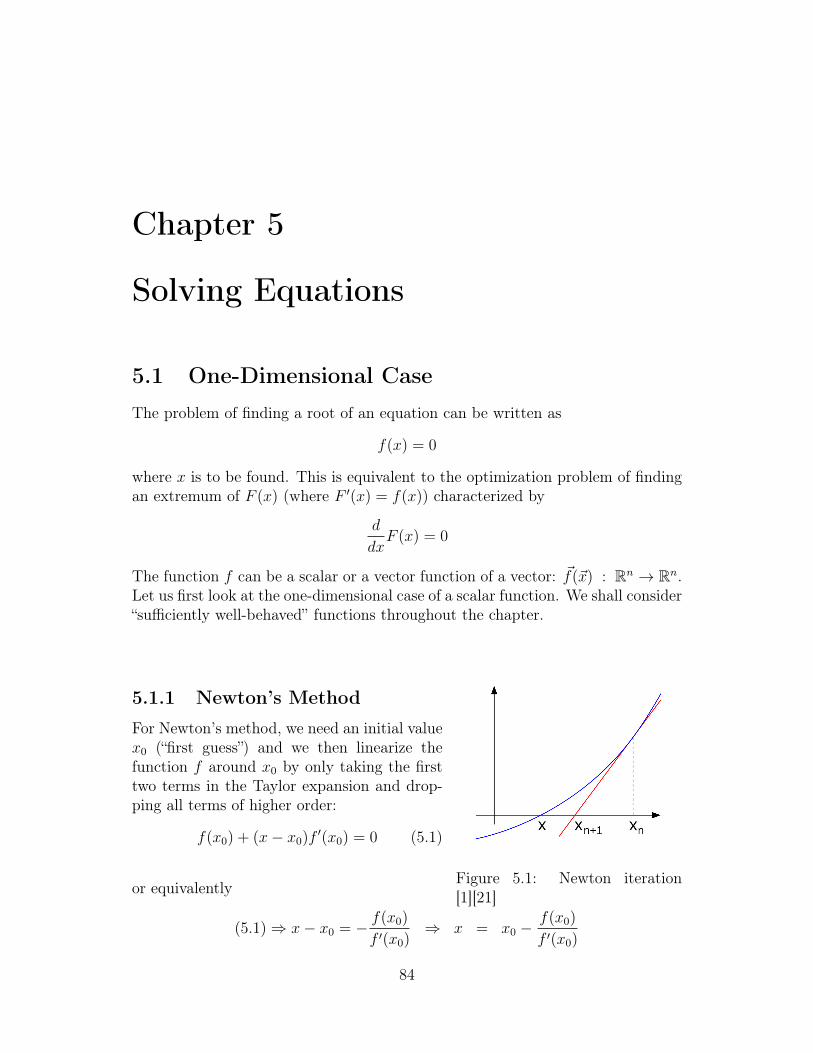
Chapter 5
Solving Equations
5.1 One-Dimensional CaseThe problem of finding a root of an equation can be written as
f(x) = 0
where x is to be found. This is equivalent to the optimization problem of findingan extremum of F (x) (where F ′(x) = f(x)) characterized by
d
dxF (x) = 0
The function f can be a scalar or a vector function of a vector: ~f(~x) : Rn → Rn.Let us first look at the one-dimensional case of a scalar function. We shall consider“sufficiently well-behaved” functions throughout the chapter.
Figure 5.1: Newton iteration[1][21]
5.1.1 Newton’s Method
For Newton’s method, we need an initial valuex0 (“first guess”) and we then linearize thefunction f around x0 by only taking the firsttwo terms in the Taylor expansion and drop-ping all terms of higher order:
f(x0) + (x− x0)f ′(x0) = 0 (5.1)
or equivalently
(5.1)⇒ x− x0 = − f(x0)
f ′(x0)⇒ x = x0 −
f(x0)
f ′(x0)
84
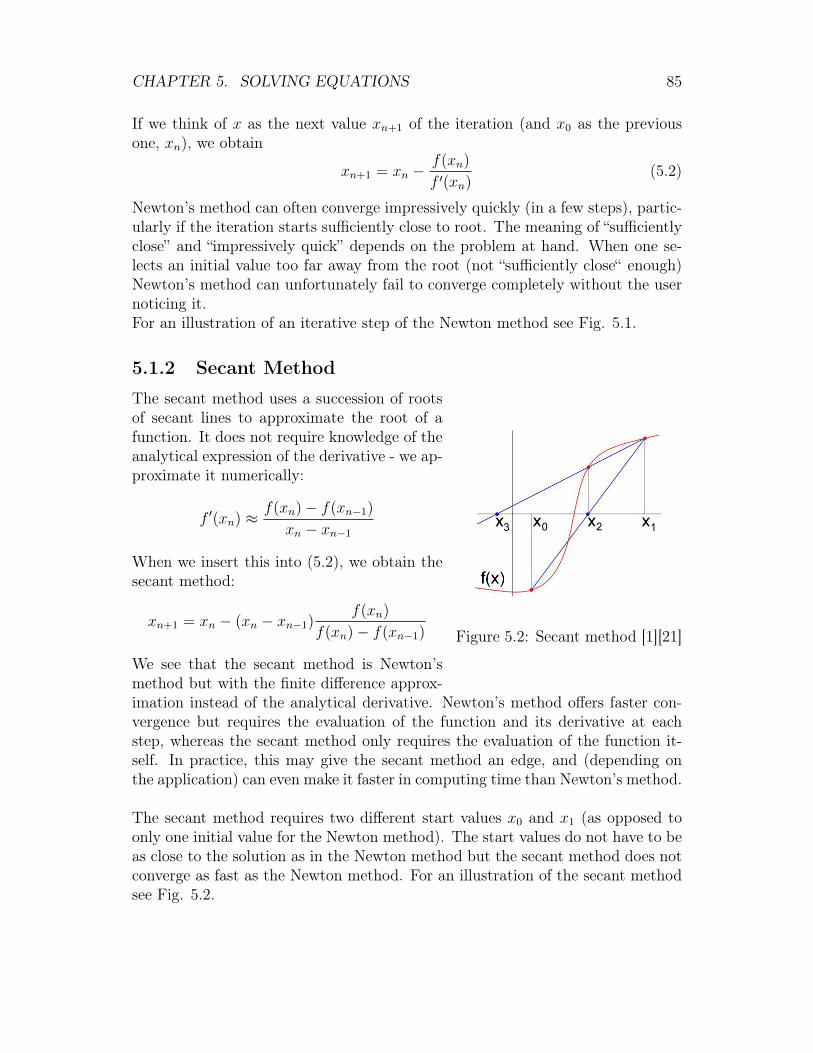
CHAPTER 5. SOLVING EQUATIONS 85
If we think of x as the next value xn+1 of the iteration (and x0 as the previousone, xn), we obtain
xn+1 = xn −f(xn)
f ′(xn)(5.2)
Newton’s method can often converge impressively quickly (in a few steps), partic-ularly if the iteration starts sufficiently close to root. The meaning of “sufficientlyclose” and “impressively quick” depends on the problem at hand. When one se-lects an initial value too far away from the root (not “sufficiently close“ enough)Newton’s method can unfortunately fail to converge completely without the usernoticing it.For an illustration of an iterative step of the Newton method see Fig. 5.1.
5.1.2 Secant Method
Figure 5.2: Secant method [1][21]
The secant method uses a succession of rootsof secant lines to approximate the root of afunction. It does not require knowledge of theanalytical expression of the derivative - we ap-proximate it numerically:
f ′(xn) ≈ f(xn)− f(xn−1)
xn − xn−1
When we insert this into (5.2), we obtain thesecant method:
xn+1 = xn − (xn − xn−1)f(xn)
f(xn)− f(xn−1)
We see that the secant method is Newton’smethod but with the finite difference approx-imation instead of the analytical derivative. Newton’s method offers faster con-vergence but requires the evaluation of the function and its derivative at eachstep, whereas the secant method only requires the evaluation of the function it-self. In practice, this may give the secant method an edge, and (depending onthe application) can even make it faster in computing time than Newton’s method.
The secant method requires two different start values x0 and x1 (as opposed toonly one initial value for the Newton method). The start values do not have to beas close to the solution as in the Newton method but the secant method does notconverge as fast as the Newton method. For an illustration of the secant methodsee Fig. 5.2.
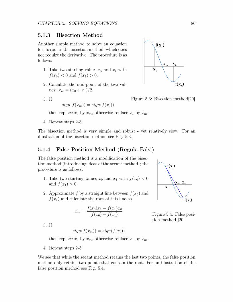
CHAPTER 5. SOLVING EQUATIONS 86
5.1.3 Bisection Method
Figure 5.3: Bisection method[20]
Another simple method to solve an equationfor its root is the bisection method, which doesnot require the derivative. The procedure is asfollows:
1. Take two starting values x0 and x1 withf(x0) < 0 and f(x1) > 0.
2. Calculate the mid-point of the two val-ues: xm = (x0 + x1)/2.
3. Ifsign(f(xm)) = sign(f(x0))
then replace x0 by xm, otherwise replace x1 by xm.
4. Repeat steps 2-3.
The bisection method is very simple and robust - yet relatively slow. For anillustration of the bisection method see Fig. 5.3.
5.1.4 False Position Method (Regula Falsi)
Figure 5.4: False posi-tion method [20]
The false position method is a modification of the bisec-tion method (introducing ideas of the secant method); theprocedure is as follows:
1. Take two starting values x0 and x1 with f(x0) < 0and f(x1) > 0.
2. Approximate f by a straight line between f(x0) andf(x1) and calculate the root of this line as
xm =f(x0)x1 − f(x1)x0
f(x0)− f(x1)
3. Ifsign(f(xm)) = sign(f(x0))
then replace x0 by xm, otherwise replace x1 by xm.
4. Repeat steps 2-3.
We see that while the secant method retains the last two points, the false positionmethod only retains two points that contain the root. For an illustration of thefalse position method see Fig. 5.4.
CHAPTER 5. SOLVING EQUATIONS 87
5.2 N-Dimensional CaseAs a generalization of the previously discussed methods, we can solve a system ofN coupled equations:
~f(~x) = 0
The corresponding N dimensional optimization problem is then~∇F (~x) = 0
where, similar to the aforementioned case, ~∇F = ~f(~x). Let us look at the neces-sary modifications.
5.2.1 Newton’s Method
Newton’s method in N dimensions replaces the derivative used in the scalar caseby the Jacobian matrix:
Jij(~x) =∂fi(~x)
∂xj
Let us consider an example: For a two dimensional function ~f , the Jacobianmatrix looks as follows:
J =
(∂f1(~x)∂x1
∂f1(~x)∂x2
∂f2(~x)∂x1
∂f2(~x)∂x2
)The Jacobian matrix needs to be non-singular and well-conditioned because itneeds to be inverted numerically. The Newton iteration condition in N dimensionsis given by
~xn+1 = ~xn − J−1 ~f(~xn) (5.3)Newton’s method in N dimensions can be interpreted as a linearization. We canshow this by solving a system of linear equations (due to the nature of the method,we should encounter the solution in exactly one step in the case of a linear equa-tion).
Consider the system of linear equations (B ∈Mn×n(R) and ~x,~c ∈ Rn)
B~x = ~c (5.4)
whose exact solution is~x = B−1~c (5.5)
The system (5.4) can also be written as
~f(~x) = B~x− c = 0 ⇒ J = B (first derivative) (5.6)
Now we apply the Newton method by inserting (5.6) into (5.3):
~xn+1 = ~xn −B−1(B~xn − ~c) = B−1~c
and have thus found the exact solution in one step.
CHAPTER 5. SOLVING EQUATIONS 88
5.2.2 Secant Method
The N -dimensional secant method is characterized by the numerically calculatedJacobi matrix (as opposed to the analytical Jacobi matrix from 5.2.1) :
Ji,j(~x) =fi(~x+ hj~ej)− fi(~x)
hj(5.7)
with ~ej the unit vector in the direction j. Insert this J into (5.3) and iterate.
hj should be chosen such that hj ≈ xj√ε, where ε is the machine precision (e.g.
10−16 for a 64-bit computer)
5.2.3 Other Techniques
We can also solve an N -dimensional system of equations with the relaxationmethod:
~f(~x) = 0→ xi = gi(xj, j 6= i), i = 1, . . . , N (5.8)
Start with xi(0) and iterate: xi(t+ 1) = gi(xj(t)).
There are also gradient methods such as the “steepest descent method” or the“conjugate gradient method”, which we are not going to go into.
Chapter 6
Ordinary Differential Equations
First order ordinary differential equations (ODE) and initial value problems canbe written as
dy
dt= f(y, t) with y(t0) = y0 (6.1)
If we want to solve an ODE numerically, we have to discretize time so that wecan advance in time steps of size ∆t.
6.1 ExamplesWe see examples of ODEs around us every day. The walls around us have slightlyradioactive material in them which obeys the equation of radioactive decay
dN
dt= −λN
with the solution N = N0e−λt. Another everyday example is the cooling of coffee
which obeys the equation
dT
dt= −γ(T − Troom)
How do we solve such equations numerically? Let us look at some methods,starting out with the Euler method.
6.2 Euler MethodThe Euler method is a simple numerical method to solve a first order ODE witha given initial value.
89
CHAPTER 6. ORDINARY DIFFERENTIAL EQUATIONS 90
The Euler recipe is as follows:
1. Take the initial value y(t0) = y0
2. Calculate dydt.
3. Advance linearly for ∆t with the derivative at the initial value as the slope:
y(t+ ∆t) = y(t) + ∆t · y′(t)
4. Take the point reached in the previous step as new initial value and repeatsteps 2-3.
Let us derive this for finite differences:We want to approximate the solution of the initial value problem
y′(t) = f(t, y(t)) , y(t0) = y0
We consider only the first two terms of the Taylor expansion and drop all higherorder terms:
y(t0 + ∆t) = y(t0) + ∆t · dydt
(t0) +O((∆t)2) = y(t0) + ∆t · f(y0, t0)︸ ︷︷ ︸≡y(t1)≡y1
+O((∆t)2)
This corresponds to a linearization around (t0, y0). One time step (with tn+1 =t0 + n ·∆t) in the Euler method corresponds to
yn+1 = yn + ∆t · f(tn, yn)
The solution yn+1 is explicit (it is an explicit function of yi, 1 ≤ i ≤ n). Whenwe start out at y0 and iterate, we will find yn; this is the simplest finite differencemethod. Unfortunately, we also accumulate an error at every time step so wegradually drift away from the exact solution (see Fig. 6.1). The error for eachtime step is ∝ (∆t)2.
6.2.1 Interlude: The Order of a Method
In the past, we have analyzed the error for many methods, so before continuing itis helpful to introduce some formalism. We say of a method that it is locally oforder n if the error at one time step is O((∆t)n). However, that is not the wholetruth as we are usually interested in the error accumulation over a fixed intervalT , consisting of m subintervals ∆t, where m is given by
m =T
∆t
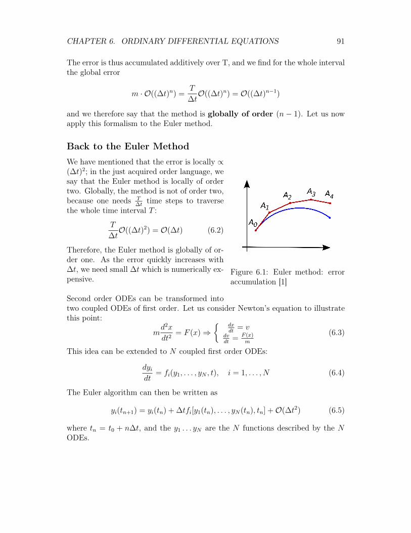
CHAPTER 6. ORDINARY DIFFERENTIAL EQUATIONS 91
The error is thus accumulated additively over T, and we find for the whole intervalthe global error
m · O((∆t)n) =T
∆tO((∆t)n) = O((∆t)n−1)
and we therefore say that the method is globally of order (n− 1). Let us nowapply this formalism to the Euler method.
Back to the Euler Method
Figure 6.1: Euler method: erroraccumulation [1]
We have mentioned that the error is locally ∝(∆t)2; in the just acquired order language, wesay that the Euler method is locally of ordertwo. Globally, the method is not of order two,because one needs T
∆ttime steps to traverse
the whole time interval T :
T
∆tO((∆t)2) = O(∆t) (6.2)
Therefore, the Euler method is globally of or-der one. As the error quickly increases with∆t, we need small ∆t which is numerically ex-pensive.
Second order ODEs can be transformed intotwo coupled ODEs of first order. Let us consider Newton’s equation to illustratethis point:
md2x
dt2= F (x)⇒
{dxdt
= vdvdt
= F (x)m
(6.3)
This idea can be extended to N coupled first order ODEs:
dyidt
= fi(y1, . . . , yN , t), i = 1, . . . , N (6.4)
The Euler algorithm can then be written as
yi(tn+1) = yi(tn) + ∆tfi[y1(tn), . . . , yN(tn), tn] +O(∆t2) (6.5)
where tn = t0 + n∆t, and the y1 . . . yN are the N functions described by the NODEs.
CHAPTER 6. ORDINARY DIFFERENTIAL EQUATIONS 92
6.3 Runge-Kutta MethodsInstead of taking increasingly small time steps to obtain a better approximationto the solution of a given ODE, we can take a completely different approach:We can improve the procedure itself instead of shortening the time steps. Ofcourse the goal of such a change of agenda is that we are not going to need smalltime steps anymore to get an accurate solution. The way to do this can be seenwhen going back to the beginning of the Euler method: Instead of dropping allbut the first two terms in the Taylor expansion, we could improve the method bygetting a better grip on the slope (better than the previous linear approximation).
The Runge-Kutta methods are a generalization of the Euler method, but theyachieve the same accuracy as the Euler method for much larger time steps. There-fore, the Runge-Kutta methods are numerically less expensive (yet more compli-cated to implement).
Formally, the Runge-Kutta methods are derived using a Taylor expansion fory(t+ ∆t) keeping all terms up to order (∆t)q:
y(t+ ∆t) = y(t) +(∆t)
1!
dy
dt+
(∆t)2
2!· d
2y
dt2+ · · ·+ (∆t)q
q!· d
qy
dtq+O((∆t)q+1) (6.6)
We are now going to look at a couple of examples of Runge-Kutta methods anddiscuss their order later on.
6.3.1 2nd Order Runge-Kutta Method
Let us start with the 2nd order Runge-Kutta method. This is the simplest exten-sion of the Euler method, where we add a term to the previously used linearization.This turns (6.6) into:
y(t+ ∆t) = y(t) +(∆t)
1!
dy
dt+
(∆t)2
2!· d
2y
dt2+O((∆t)3)
We can now formulate the iteration recipe for the 2nd order Runge-Kutta method:
1. Perform an Euler step of size ∆t2, starting at the initial value yi(t0):
yi
(t+
1
2∆t
)= yi(t) +
1
2∆tf [yi(t), t]
2. Calculate the derivative at the reached point.
3. Advance a full time step with the calculated derivative as slope.
4. Take the reached point as initial value and repeat steps 1 to 3.
CHAPTER 6. ORDINARY DIFFERENTIAL EQUATIONS 93
This leads to the following iteration:
yi(t+ ∆t) = yi(t) + ∆tf
[yi
(t+
1
2∆t
), t+
1
2∆t
]+O((∆t)3) (6.7)
This is not the most commonly used Runge-Kutta method though. Most appli-cations using Runge-Kutta have an implementation of the 4th order Runge-Kuttamethod.
6.3.2 4th Order Runge-Kutta Method
There exist more optimized versions of the Runge-Kutta method than the 2nd
order one. A commonly used implementation is the so-called RK4 which is a 4th
order Runge-Kutta method.
The procedure is as follows:
1. Define 4 coefficients:
k1 = f(yn, tn)
k2 = f(yn + 1
2∆t · k1, tn + 1
2∆t)
k3 = f(yn + 1
2∆t · k2, tn + 1
2∆t)
k4 = f(yn + ∆t · k3, tn + ∆t)
2. Calculate the next step using a weighted sum of the defined coefficients:
yn+1 = yn + ∆t ·(
1
6k1 +
1
3k2 +
1
3k3 +
1
6k4
)+O((∆t)5) (6.8)
As you can see, the weighting factors are chosen in such a way that the sumof them is 1: 1
6+ 1
3+ 1
3+ 1
6= 1
This method is globally of order 4 and locally of order 5. The selection of theweighting factors is not unique (see section 6.3.4).
6.3.3 q-Stage Runge-Kutta Method
The definition of the Runge-Kutta methods is more general than what we haveseen so far. They are defined by the so called stage, which determines the numberof terms in the sum of the iteration formula:
yn+1 = yn + ∆t ·q∑i=1
ωiki (6.9)
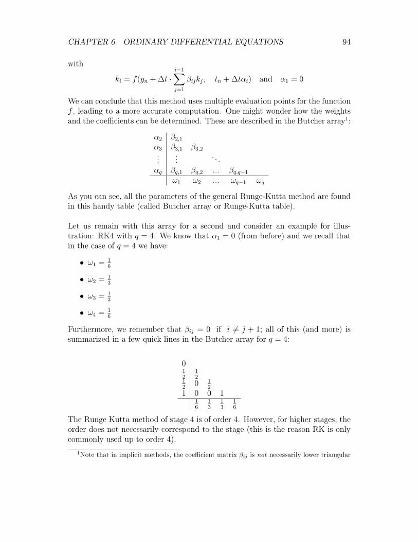
CHAPTER 6. ORDINARY DIFFERENTIAL EQUATIONS 94
with
ki = f(yn + ∆t ·i−1∑j=1
βijkj, tn + ∆tαi) and α1 = 0
We can conclude that this method uses multiple evaluation points for the functionf , leading to a more accurate computation. One might wonder how the weightsand the coefficients can be determined. These are described in the Butcher array1:
α2 β2,1
α3 β3,1 β3,2...
... . . .αq βq,1 βq,2 ... βq,q−1
ω1 ω2 ... ωq−1 ωq
As you can see, all the parameters of the general Runge-Kutta method are foundin this handy table (called Butcher array or Runge-Kutta table).
Let us remain with this array for a second and consider an example for illus-tration: RK4 with q = 4. We know that α1 = 0 (from before) and we recall thatin the case of q = 4 we have:
• ω1 = 16
• ω2 = 13
• ω3 = 13
• ω4 = 16
Furthermore, we remember that βij = 0 if i 6= j + 1; all of this (and more) issummarized in a few quick lines in the Butcher array for q = 4:
012
12
12
0 12
1 0 0 116
13
13
16
The Runge Kutta method of stage 4 is of order 4. However, for higher stages, theorder does not necessarily correspond to the stage (this is the reason RK is onlycommonly used up to order 4).
1Note that in implicit methods, the coefficient matrix βij is not necessarily lower triangular
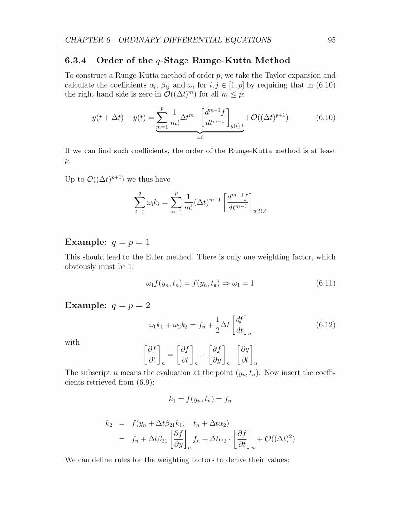
CHAPTER 6. ORDINARY DIFFERENTIAL EQUATIONS 95
6.3.4 Order of the q-Stage Runge-Kutta Method
To construct a Runge-Kutta method of order p, we take the Taylor expansion andcalculate the coefficients αi, βij and ωi for i, j ∈ [1, p] by requiring that in (6.10)the right hand side is zero in O((∆t)m) for all m ≤ p:
y(t+ ∆t)− y(t) =
p∑m=1
1
m!∆tm ·
[dm−1f
dtm−1
]y(t),t︸ ︷︷ ︸
=0
+O((∆t)p+1) (6.10)
If we can find such coefficients, the order of the Runge-Kutta method is at leastp.
Up to O((∆t)p+1) we thus have
q∑i=1
ωiki =
p∑m=1
1
m!(∆t)m−1
[dm−1f
dtm−1
]y(t),t
Example: q = p = 1
This should lead to the Euler method. There is only one weighting factor, whichobviously must be 1:
ω1f(yn, tn) = f(yn, tn)⇒ ω1 = 1 (6.11)
Example: q = p = 2
ω1k1 + ω2k2 = fn +1
2∆t
[df
dt
]n
(6.12)
with [∂f
∂t
]n
=
[∂f
∂t
]n
+
[∂f
∂y
]n
·[∂y
∂t
]n
The subscript n means the evaluation at the point (yn, tn). Now insert the coeffi-cients retrieved from (6.9):
k1 = f(yn, tn) = fn
k2 = f(yn + ∆tβ21k1, tn + ∆tα2)
= fn + ∆tβ21
[∂f
∂y
]n
fn + ∆tα2 ·[∂f
∂t
]n
+O((∆t)2)
We can define rules for the weighting factors to derive their values:
CHAPTER 6. ORDINARY DIFFERENTIAL EQUATIONS 96
• The first rule holds for all Runge-Kutta methods: the sum of the weightingfactors must be 1.
ω1 + ω2 = 1
• We obtain the second rule by comparing the coefficients in (6.12): we noticethat
[∂f∂t
]nshows up with a prefactor of 1
2. In order to get the same factor
on the left hand side, we require
ω2 · α2 =1
2
• In a similar way we can show that
ω2 · β21 =1
2
We have found three rules for four parameters. Therefore, the selection of param-eters fulfilling all conditions is not unique. However, all choices deliver a methodof the demanded order, by construction.
6.3.5 Error Estimation
The estimation of the error of a method is essential if one wants to achieve anaccurrate result in the shortest time possible.
However, that is not all that can be done with errors: Imagine we knew the exacterror (i.e. the difference between our computed result and the true result). Wewould then be able to solve the problem exactly after only one step! Unfortunately,we cannot calculate the real error, but we can try to estimate it and adapt ourmethod using the estimated error. The predictor-corrector method discussed inthis section will implement this idea to improve the previously discussed methods.
6.3.5.1 Improve Methods Using Error Estimation
As a first estimate, we define the difference between the value after two time steps∆t (called y2) and the value obtained by performing one time step of size 2∆t(called y1):
δ = y1 − y2 (6.13)
If we consider a method or order p, this definition leads to
y(t+ 2∆t) =
{y1 + (2∆t)p+1Φ +O((∆t)p+2)y2 + 2(∆t)p+1Φ +O((∆t)p+2)
(6.14)
⇒ δ = (2p+1 − 2)(∆t)p+1Φ +O((∆t)p+2) (6.15)
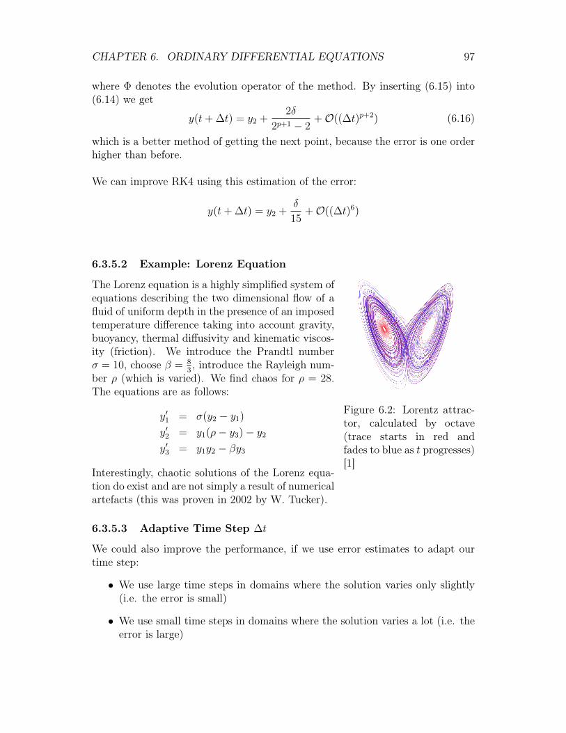
CHAPTER 6. ORDINARY DIFFERENTIAL EQUATIONS 97
where Φ denotes the evolution operator of the method. By inserting (6.15) into(6.14) we get
y(t+ ∆t) = y2 +2δ
2p+1 − 2+O((∆t)p+2) (6.16)
which is a better method of getting the next point, because the error is one orderhigher than before.
We can improve RK4 using this estimation of the error:
y(t+ ∆t) = y2 +δ
15+O((∆t)6)
Figure 6.2: Lorentz attrac-tor, calculated by octave(trace starts in red andfades to blue as t progresses)[1]
6.3.5.2 Example: Lorenz Equation
The Lorenz equation is a highly simplified system ofequations describing the two dimensional flow of afluid of uniform depth in the presence of an imposedtemperature difference taking into account gravity,buoyancy, thermal diffusivity and kinematic viscos-ity (friction). We introduce the Prandtl numberσ = 10, choose β = 8
3, introduce the Rayleigh num-
ber ρ (which is varied). We find chaos for ρ = 28.The equations are as follows:
y′1 = σ(y2 − y1)
y′2 = y1(ρ− y3)− y2
y′3 = y1y2 − βy3
Interestingly, chaotic solutions of the Lorenz equa-tion do exist and are not simply a result of numericalartefacts (this was proven in 2002 by W. Tucker).
6.3.5.3 Adaptive Time Step ∆t
We could also improve the performance, if we use error estimates to adapt ourtime step:
• We use large time steps in domains where the solution varies only slightly(i.e. the error is small)
• We use small time steps in domains where the solution varies a lot (i.e. theerror is large)
CHAPTER 6. ORDINARY DIFFERENTIAL EQUATIONS 98
First, we define the largest error that we want to accept, δexpected and we thenmeasure the real error δmeasured. The time step can then be defined as
∆tnew = ∆told
(δexpectedδmeasured
) 1p+1
(6.17)
because δ ∝ (∆t)p+1
6.3.6 Predictor-Corrector Method
Starting from the error estimation, we can define a new method of improvementfor the solution of an ODE: the predictor-corrector method. The idea is to carryout an Euler step with the mean value of the function value at time t and thefunction value at time t+ ∆t:
y(t+ ∆t) ≈ y(t) + ∆t · f(y(t)) + f(y(t+ ∆t))
2(6.18)
This is an implicit equation, which we cannot solve directly. We make a predictionof y(t+ ∆t) using the Taylor expansion of the function:
yp(t+ ∆t) = y(t) + ∆t · dydt
(t) +O((∆t)2) (6.19)
We can compute y(t+ ∆t) in (6.18) using (6.19):
yc(t+ ∆t) = y(t) + ∆t · f(y(t)) + f(yp(t+ ∆t))
2+O((∆t)3) (6.20)
The corrected value yc(t + ∆t) can itself be inserted into the corrector as thepredicted value for a better result. In fact, this can be done several times.
6.3.6.1 Higher Order Predictor-Corrector Methods
The predictor-corrector method can be extended to higher orders if we take moreterms of the Taylor expansion for the predictor, for example 4 terms for the 3rd
order predictor-corrector method:
yp(t+ ∆t) = y(t) +(∆t)
1!
dy
dt(t) +
(∆t)2
2!
d2y
dt2(t) +
(∆t)3
3!
d3y
dt3(t) +O((∆t)4) (6.21)
The computation of the corrector then becomes a bit more complicated as weneed to define one corrector for the function and two for its derivatives.
Instead of (6.20) we use (dy
dt
)c(t+ ∆t) = f(yp(t+ ∆t)) (6.22)
CHAPTER 6. ORDINARY DIFFERENTIAL EQUATIONS 99
The error is then defined as
δ =
(dy
dt
)c(t+ ∆t)−
(dy
dt
)p(t+ ∆t) (6.23)
We have to adapt the function itself and its second and third derivative in orderto get a complete corrector:
yc(t+ ∆t) = yp + c0δ(d2y
dt2
)c(t+ ∆t) =
(d2y
dt2
)p+ c2δ(
d3y
dt3
)c(t+ ∆t) =
(d3y
dt3
)p+ c3δ
with the so called Gear coefficients
c0 =3
8, c2 =
3
4, c3 =
1
6
These are obtained in a similar way to the RK coefficients in 6.3.4 by requiring themethod to be of a certain order. There are also higher order predictor-correctormethods, but the complexity increases very quickly. To get an impression of theensuing complexity, let us quickly look at the 5th order predictor-corrector method:
Of course, what we know so far is still true even for the 5th order; We have
~r1 = (δt)
(d~r0
dt
)~r2 =
1
2(δt)2
(d2~r0
dt2
)...
~rn =1
n!(δt)n
(dn~r0
dtn
)and the predictor is then given by
~r p0 (t+ δt)~r p1 (t+ δt)~r p2 (t+ δt)~r p3 (t+ δt)~r p4 (t+ δt)~r p5 (t+ δt)
=
1 1 1 1 1 10 1 2 3 4 50 0 1 3 6 100 0 0 1 4 100 0 0 0 1 50 0 0 0 0 1
~r0(t)~r1(t)~r2(t)~r3(t)~r4(t)~r5(t)
with the 1st order equation
dr
dt= f(r) ⇒ r c1 = f(r p0 ) ⇒ ∆r = r c1 − r
p1
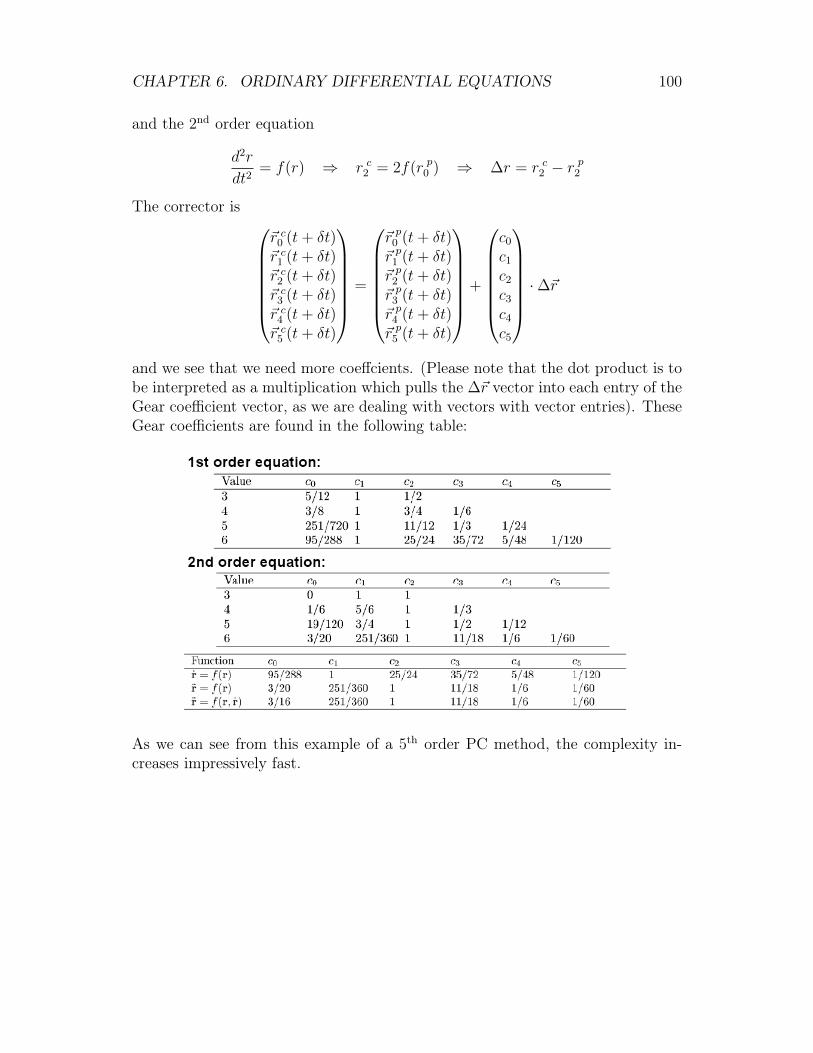
CHAPTER 6. ORDINARY DIFFERENTIAL EQUATIONS 100
and the 2nd order equation
d2r
dt2= f(r) ⇒ r c2 = 2f(r p0 ) ⇒ ∆r = r c2 − r
p2
The corrector is ~r c0 (t+ δt)~r c1 (t+ δt)~r c2 (t+ δt)~r c3 (t+ δt)~r c4 (t+ δt)~r c5 (t+ δt)
=
~r p0 (t+ δt)~r p1 (t+ δt)~r p2 (t+ δt)~r p3 (t+ δt)~r p4 (t+ δt)~r p5 (t+ δt)
+
c0
c1
c2
c3
c4
c5
·∆~r
and we see that we need more coeffcients. (Please note that the dot product is tobe interpreted as a multiplication which pulls the ∆~r vector into each entry of theGear coefficient vector, as we are dealing with vectors with vector entries). TheseGear coefficients are found in the following table:
As we can see from this example of a 5th order PC method, the complexity in-creases impressively fast.
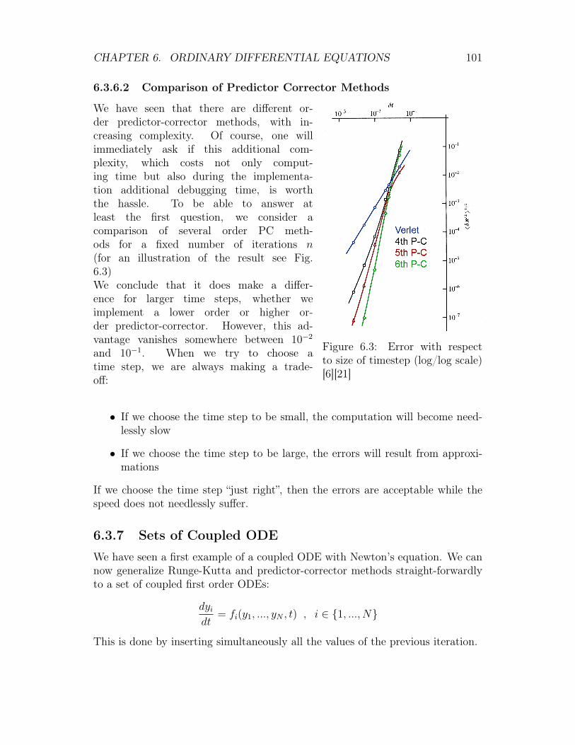
CHAPTER 6. ORDINARY DIFFERENTIAL EQUATIONS 101
6.3.6.2 Comparison of Predictor Corrector Methods
Figure 6.3: Error with respectto size of timestep (log/log scale)[6][21]
We have seen that there are different or-der predictor-corrector methods, with in-creasing complexity. Of course, one willimmediately ask if this additional com-plexity, which costs not only comput-ing time but also during the implementa-tion additional debugging time, is worththe hassle. To be able to answer atleast the first question, we consider acomparison of several order PC meth-ods for a fixed number of iterations n(for an illustration of the result see Fig.6.3)We conclude that it does make a differ-ence for larger time steps, whether weimplement a lower order or higher or-der predictor-corrector. However, this ad-vantage vanishes somewhere between 10−2
and 10−1. When we try to choose atime step, we are always making a trade-off:
• If we choose the time step to be small, the computation will become need-lessly slow
• If we choose the time step to be large, the errors will result from approxi-mations
If we choose the time step “just right”, then the errors are acceptable while thespeed does not needlessly suffer.
6.3.7 Sets of Coupled ODE
We have seen a first example of a coupled ODE with Newton’s equation. We cannow generalize Runge-Kutta and predictor-corrector methods straight-forwardlyto a set of coupled first order ODEs:
dyidt
= fi(y1, ..., yN , t) , i ∈ {1, ..., N}
This is done by inserting simultaneously all the values of the previous iteration.
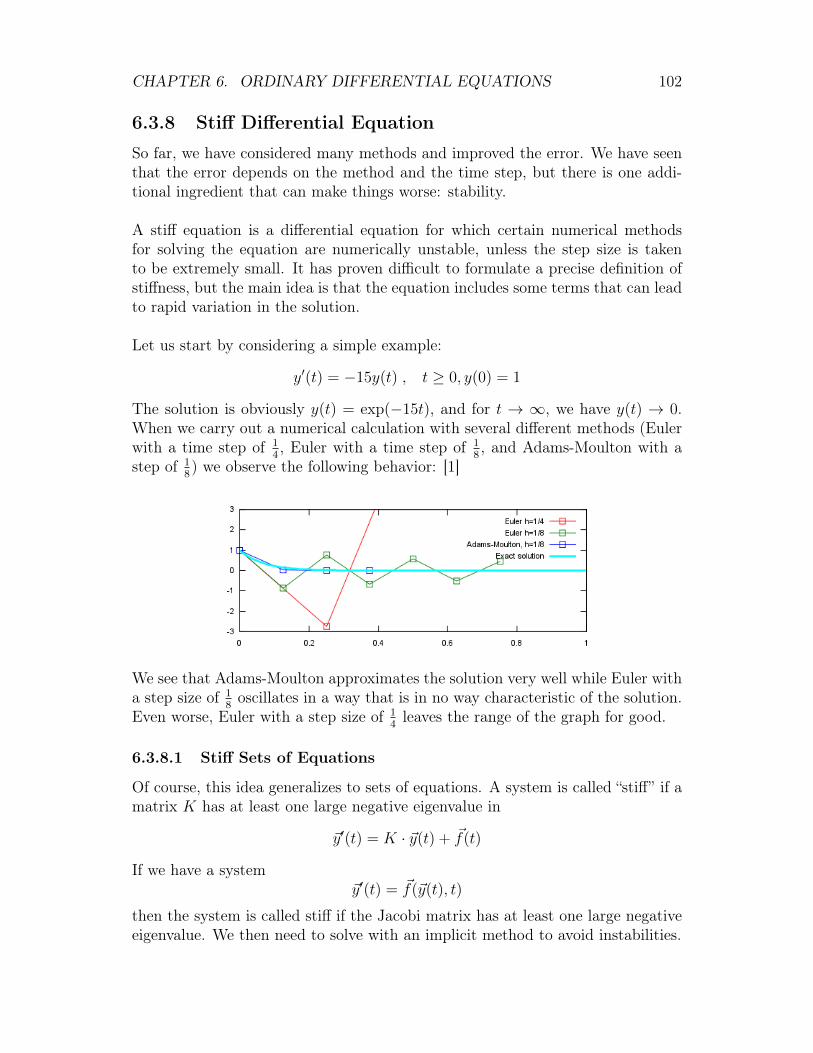
CHAPTER 6. ORDINARY DIFFERENTIAL EQUATIONS 102
6.3.8 Stiff Differential Equation
So far, we have considered many methods and improved the error. We have seenthat the error depends on the method and the time step, but there is one addi-tional ingredient that can make things worse: stability.
A stiff equation is a differential equation for which certain numerical methodsfor solving the equation are numerically unstable, unless the step size is takento be extremely small. It has proven difficult to formulate a precise definition ofstiffness, but the main idea is that the equation includes some terms that can leadto rapid variation in the solution.
Let us start by considering a simple example:
y′(t) = −15y(t) , t ≥ 0, y(0) = 1
The solution is obviously y(t) = exp(−15t), and for t → ∞, we have y(t) → 0.When we carry out a numerical calculation with several different methods (Eulerwith a time step of 1
4, Euler with a time step of 1
8, and Adams-Moulton with a
step of 18) we observe the following behavior: [1]
We see that Adams-Moulton approximates the solution very well while Euler witha step size of 1
8oscillates in a way that is in no way characteristic of the solution.
Even worse, Euler with a step size of 14leaves the range of the graph for good.
6.3.8.1 Stiff Sets of Equations
Of course, this idea generalizes to sets of equations. A system is called “stiff” if amatrix K has at least one large negative eigenvalue in
~y′(t) = K · ~y(t) + ~f(t)
If we have a system~y′(t) = ~f(~y(t), t)
then the system is called stiff if the Jacobi matrix has at least one large negativeeigenvalue. We then need to solve with an implicit method to avoid instabilities.
CHAPTER 6. ORDINARY DIFFERENTIAL EQUATIONS 103
Literature• G.E. Forsythe, M.A. Malcolm and C.B. Moler, “Computer Methods for
Mathematical Computations” (Prentice Hall, Englewood Cliffs, NJ, 1977),Chapter 6
• E.Hairer, S.P. Norsett and G. Wanner, “Solving Ordinary Differential Equa-tions I” (Springer, Berlin, 1993)
• W.H. Press, B.P.Flanery, S.A. Teukolsky and W.T. Vetterling, “NumericalRecipes” (Cabridge University Press, Cambridge, 1988) Sect. 16.1 and 16.2
• J.C. Butcher, “The Numerical Analysis of Ordinary Differential Equations”(Wiley, New York, 1987)
• J.D. Lambert, “Numerical Methods for Ordinary Differential Equations”(John Wiley & Sons, New York, 1991)
• L.F. Shampine, “Numerical Solution of Ordinary Differential Equations”(Chapman and Hall, London, 1994)
Chapter 7
Partial Differential Equations
A partial differential equation (PDE) is a differential equation involving an un-known function of several independent variables (including the unknown function’sderivatives with respect to the parameters).
To warm up, let us consider a very simple example:
∂
∂xu(x, y) = 0
We immediately see that the function u(x, y) has no x-dependence and can thusbe written as u(x, y) = f(y), where f(y) is just an arbitrary function of y. Ofcourse, the same idea can also be done with swapped variables,
∂
∂yv(x, y) = 0
with the solution v(x, y) = f(x) as in this example v(x, y) has no y-dependence.Keeping this rather trivial example in mind, we would like to find a more generalexpression to characterize partial differential equations so that we are able to workwith just about any PDE.
7.1 Types of PDEsIn the introductory example, we considered only first derivatives with respect tothe position. In general, time may also be a variable and we are not limited to firstderivatives. In fact, we are also going to allow second derivatives and an additionalfunction. In such a more general expression (with up to second derivatives), allof these six terms (∂xu , ∂2
xu , ∂tu , ∂2t u , ∂x∂tu , f) appear with a coefficient
(which can be position and time dependent). We can now write out the general
104
CHAPTER 7. PARTIAL DIFFERENTIAL EQUATIONS 105
form of the definition of such a PDE with two variables:
a(x, t)∂2u(x, t)
∂x2+ b(x, t)
∂2u(x, t)
∂x∂t+ c(x, t)
∂2u(x, t)
∂t2+
d(x, t)∂u(x, t)
∂x+ e(x, t)
∂u(x, t)
∂t+ f(u, x, t) = 0
Based on the coefficients, we distinguish three types of PDEs:
1. A PDE is elliptic, if
a(x, t)c(x, t)− b(x, t)2
4> 0 (7.1)
2. A PDE is parabolic, if
a(x, t)c(x, t)− b(x, t)2
4= 0 (7.2)
3. A PDE is hyperbolic, if
a(x, t)c(x, t)− b(x, t)2
4< 0 (7.3)
Let us apply this knowledge to a couple of examples.
7.2 Examples of PDEs
7.2.1 Scalar Boundary Value Problems (Elliptic PDEs)
The elliptic PDEs can be further subcategorized based on their boundary condi-tions. There are two boundary conditions:
• The Dirichlet problem has a fixed value on the boundary Γ:
f(x)|Γ = y0
• The von Neumann problem has a fixed gradient on the boundary Γ:
∇f(x)|Γ = y0
To illustrate this point, let us try to identify the Poisson and the Laplace equation:
• The Poisson equation is
∆Φ = ρ(~x), Φ(x)|Γ = Φ0
with the charge distribution ρ(~x) and the fixed value Φ0 on the boundary Γ.Obviously, the Poisson equation is a Dirichlet problem since the value (notthe gradient) is fixed on the boundaries.
CHAPTER 7. PARTIAL DIFFERENTIAL EQUATIONS 106
• The Laplace equation is
∆Φ = 0, ∇nΦ(x)|Γ = Ψ0
with the fixed value Ψ0 of the gradient of Φ on the boundary Γ. We im-mediately recognize the von Neumann character of this equation, since thegradient is fixed and not the value.
7.2.2 Vectorial Boundary Value Problem
An example of a vectorial boundary value problem is the Lamé equation of elas-ticity, which is an elliptic boundary value problem.
Consider a homogeneous isotropic medium G ∈ Rn with a boundary Γ, whosestate (in the absence of body forces) is given by the Lamé equation:
~∇(~∇~u(~x)) + (1− ν)∆~u(~x) = 0 (7.4)
where ~u(x) = (u1(x1, ..., xn), ..., un(x1, ..., xn)) is a vector of displacements and νis the Poisson ratio, which describes how much the material gets thinner in twodimensions if you stretch it in the third one.
7.2.3 Wave Equation
The wave equation describes a wave traveling at a speed cp; it is a second orderlinear partial differential equation. One can use it e.g. for sound, light and waterwaves.
The wave equation is a typical example of a hyperbolic PDE. Let us considerthe simplest form, where u is a scalar function u = u(x, t) which satisfies
∂2u(~x, t)
∂t2= cp
2 ∆u(~x, t) (7.5)
with the initial conditionu(~x, t0) = u0(~x)
The fixed constant cp corresponds to the propagation speed of the wave, e.g. thespeed of sound for acoustic waves. We see that when we consider the coefficientsin the general form of a PDE, only the following coefficients are non-zero:
• c(~x, t): the equation contains a ∂2t u expression
• a(~x, t): the equation contains a ∂2xu expression
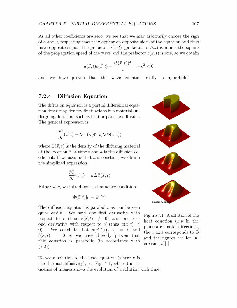
CHAPTER 7. PARTIAL DIFFERENTIAL EQUATIONS 107
As all other coefficients are zero, we see that we may arbitrarily choose the signof a and c, respecting that they appear on opposite sides of the equation and thushave opposite signs. The prefactor a(x, t) (prefactor of ∆u) is minus the squareof the propagation speed of the wave and the prefactor c(x, t) is one, so we obtain
a(~x, t)c(~x, t)− (b(~x, t))2
4= −c2 < 0
and we have proven that the wave equation really is hyperbolic.
Figure 7.1: A solution of theheat equation (x,y in theplane are spatial directions,the z axis corresponds to Φand the figures are for in-creasing t)[1]
7.2.4 Diffusion Equation
The diffusion equation is a partial differential equa-tion describing density fluctuations in a material un-dergoing diffusion, such as heat or particle diffusion.The general expression is
∂Φ
∂t(~x, t) = ∇ · (κ(Φ, ~x)∇Φ(~x, t))
where Φ(~x, t) is the density of the diffusing materialat the location ~x at time t and κ is the diffusion co-efficient. If we assume that κ is constant, we obtainthe simplified expression
∂Φ
∂t(~x, t) = κ∆Φ(~x, t)
Either way, we introduce the boundary condition
Φ(~x, t)|Γ = Φ0(t)
The diffusion equation is parabolic as can be seenquite easily. We have one first derivative withrespect to t (thus e(~x, t) 6= 0) and one sec-ond derivative with respect to ~x (thus a(~x, t) 6=0). We conclude that a(~x, t)c(~x, t) = 0 andb(x, t) = 0 so we have directly proven thatthis equation is parabolic (in accordance with(7.2)).
To see a solution to the heat equation (where κ isthe thermal diffusivity), see Fig. 7.1, where the se-quence of images shows the evolution of a solution with time.
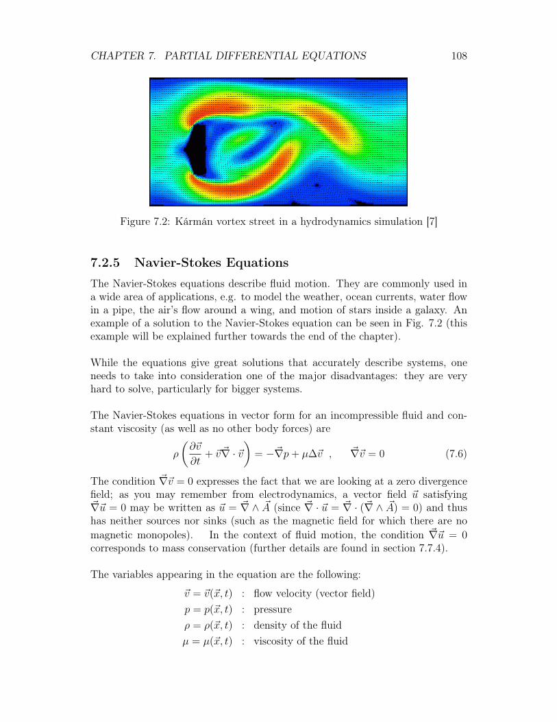
CHAPTER 7. PARTIAL DIFFERENTIAL EQUATIONS 108
Figure 7.2: Kármán vortex street in a hydrodynamics simulation [7]
7.2.5 Navier-Stokes Equations
The Navier-Stokes equations describe fluid motion. They are commonly used ina wide area of applications, e.g. to model the weather, ocean currents, water flowin a pipe, the air’s flow around a wing, and motion of stars inside a galaxy. Anexample of a solution to the Navier-Stokes equation can be seen in Fig. 7.2 (thisexample will be explained further towards the end of the chapter).
While the equations give great solutions that accurately describe systems, oneneeds to take into consideration one of the major disadvantages: they are veryhard to solve, particularly for bigger systems.
The Navier-Stokes equations in vector form for an incompressible fluid and con-stant viscosity (as well as no other body forces) are
ρ
(∂~v
∂t+ ~v~∇ · ~v
)= −~∇p+ µ∆~v , ~∇~v = 0 (7.6)
The condition ~∇~v = 0 expresses the fact that we are looking at a zero divergencefield; as you may remember from electrodynamics, a vector field ~u satisfying~∇~u = 0 may be written as ~u = ~∇ ∧ ~A (since ~∇ · ~u = ~∇ · (~∇ ∧ ~A) = 0) and thushas neither sources nor sinks (such as the magnetic field for which there are nomagnetic monopoles). In the context of fluid motion, the condition ~∇~u = 0corresponds to mass conservation (further details are found in section 7.7.4).
The variables appearing in the equation are the following:
~v = ~v(~x, t) : flow velocity (vector field)p = p(~x, t) : pressureρ = ρ(~x, t) : density of the fluidµ = µ(~x, t) : viscosity of the fluid
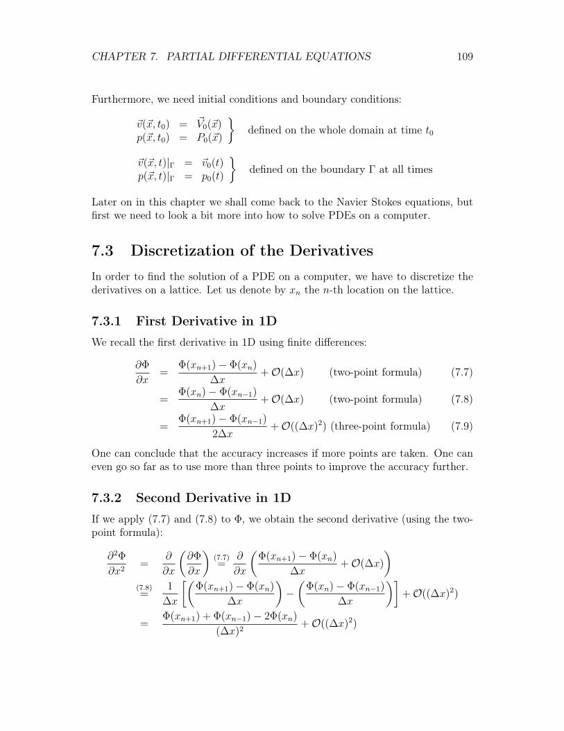
CHAPTER 7. PARTIAL DIFFERENTIAL EQUATIONS 109
Furthermore, we need initial conditions and boundary conditions:
~v(~x, t0) = ~V0(~x)p(~x, t0) = P0(~x)
}defined on the whole domain at time t0
~v(~x, t)|Γ = ~v0(t)p(~x, t)|Γ = p0(t)
}defined on the boundary Γ at all times
Later on in this chapter we shall come back to the Navier Stokes equations, butfirst we need to look a bit more into how to solve PDEs on a computer.
7.3 Discretization of the DerivativesIn order to find the solution of a PDE on a computer, we have to discretize thederivatives on a lattice. Let us denote by xn the n-th location on the lattice.
7.3.1 First Derivative in 1D
We recall the first derivative in 1D using finite differences:
∂Φ
∂x=
Φ(xn+1)− Φ(xn)
∆x+O(∆x) (two-point formula) (7.7)
=Φ(xn)− Φ(xn−1)
∆x+O(∆x) (two-point formula) (7.8)
=Φ(xn+1)− Φ(xn−1)
2∆x+O((∆x)2) (three-point formula) (7.9)
One can conclude that the accuracy increases if more points are taken. One caneven go so far as to use more than three points to improve the accuracy further.
7.3.2 Second Derivative in 1D
If we apply (7.7) and (7.8) to Φ, we obtain the second derivative (using the two-point formula):
∂2Φ
∂x2=
∂
∂x
(∂Φ
∂x
)(7.7)=
∂
∂x
(Φ(xn+1)− Φ(xn)
∆x+O(∆x)
)(7.8)=
1
∆x
[(Φ(xn+1)− Φ(xn)
∆x
)−(
Φ(xn)− Φ(xn−1)
∆x
)]+O((∆x)2)
=Φ(xn+1) + Φ(xn−1)− 2Φ(xn)
(∆x)2+O((∆x)2)
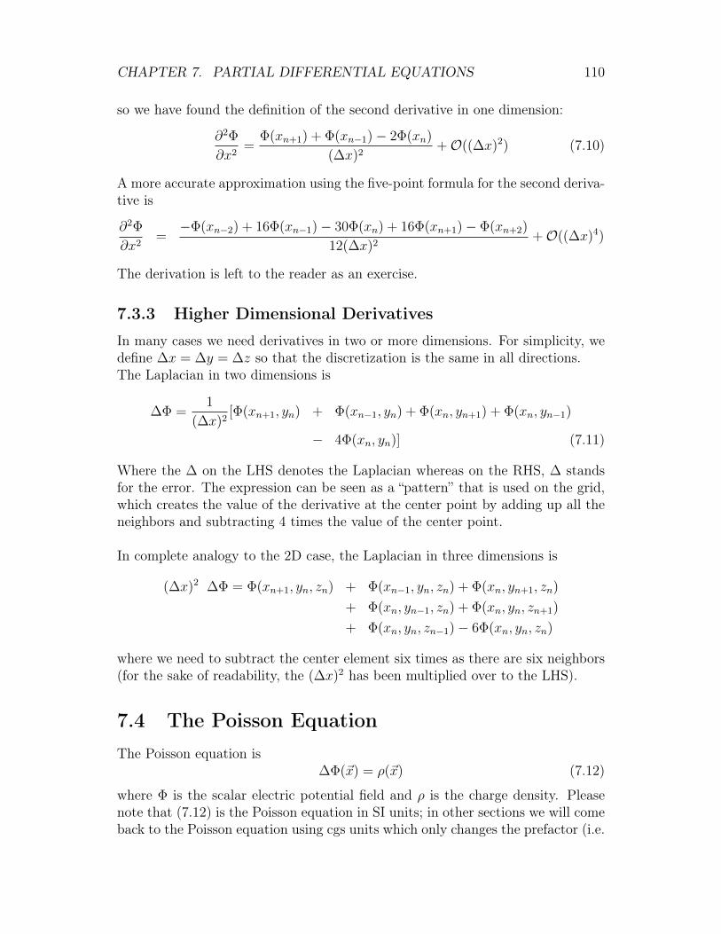
CHAPTER 7. PARTIAL DIFFERENTIAL EQUATIONS 110
so we have found the definition of the second derivative in one dimension:
∂2Φ
∂x2=
Φ(xn+1) + Φ(xn−1)− 2Φ(xn)
(∆x)2+O((∆x)2) (7.10)
A more accurate approximation using the five-point formula for the second deriva-tive is
∂2Φ
∂x2=−Φ(xn−2) + 16Φ(xn−1)− 30Φ(xn) + 16Φ(xn+1)− Φ(xn+2)
12(∆x)2+O((∆x)4)
The derivation is left to the reader as an exercise.
7.3.3 Higher Dimensional Derivatives
In many cases we need derivatives in two or more dimensions. For simplicity, wedefine ∆x = ∆y = ∆z so that the discretization is the same in all directions.The Laplacian in two dimensions is
∆Φ =1
(∆x)2[Φ(xn+1, yn) + Φ(xn−1, yn) + Φ(xn, yn+1) + Φ(xn, yn−1)
− 4Φ(xn, yn)] (7.11)
Where the ∆ on the LHS denotes the Laplacian whereas on the RHS, ∆ standsfor the error. The expression can be seen as a “pattern” that is used on the grid,which creates the value of the derivative at the center point by adding up all theneighbors and subtracting 4 times the value of the center point.
In complete analogy to the 2D case, the Laplacian in three dimensions is
(∆x)2 ∆Φ = Φ(xn+1, yn, zn) + Φ(xn−1, yn, zn) + Φ(xn, yn+1, zn)
+ Φ(xn, yn−1, zn) + Φ(xn, yn, zn+1)
+ Φ(xn, yn, zn−1)− 6Φ(xn, yn, zn)
where we need to subtract the center element six times as there are six neighbors(for the sake of readability, the (∆x)2 has been multiplied over to the LHS).
7.4 The Poisson EquationThe Poisson equation is
∆Φ(~x) = ρ(~x) (7.12)
where Φ is the scalar electric potential field and ρ is the charge density. Pleasenote that (7.12) is the Poisson equation in SI units; in other sections we will comeback to the Poisson equation using cgs units which only changes the prefactor (i.e.
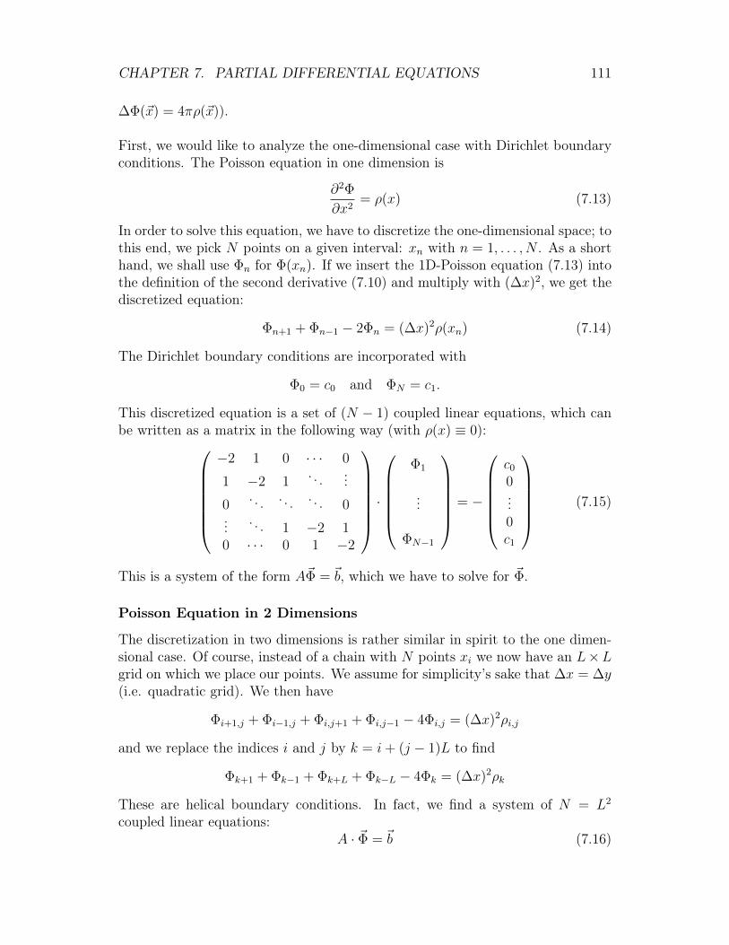
CHAPTER 7. PARTIAL DIFFERENTIAL EQUATIONS 111
∆Φ(~x) = 4πρ(~x)).
First, we would like to analyze the one-dimensional case with Dirichlet boundaryconditions. The Poisson equation in one dimension is
∂2Φ
∂x2= ρ(x) (7.13)
In order to solve this equation, we have to discretize the one-dimensional space; tothis end, we pick N points on a given interval: xn with n = 1, . . . , N . As a shorthand, we shall use Φn for Φ(xn). If we insert the 1D-Poisson equation (7.13) intothe definition of the second derivative (7.10) and multiply with (∆x)2, we get thediscretized equation:
Φn+1 + Φn−1 − 2Φn = (∆x)2ρ(xn) (7.14)
The Dirichlet boundary conditions are incorporated with
Φ0 = c0 and ΦN = c1.
This discretized equation is a set of (N − 1) coupled linear equations, which canbe written as a matrix in the following way (with ρ(x) ≡ 0):
−2 1 0 · · · 0
1 −2 1. . . ...
0. . . . . . . . . 0
... . . . 1 −2 10 · · · 0 1 −2
·
Φ1
...
ΦN−1
= −
c0
0...0c1
(7.15)
This is a system of the form A~Φ = ~b, which we have to solve for ~Φ.
Poisson Equation in 2 Dimensions
The discretization in two dimensions is rather similar in spirit to the one dimen-sional case. Of course, instead of a chain with N points xi we now have an L×Lgrid on which we place our points. We assume for simplicity’s sake that ∆x = ∆y(i.e. quadratic grid). We then have
Φi+1,j + Φi−1,j + Φi,j+1 + Φi,j−1 − 4Φi,j = (∆x)2ρi,j
and we replace the indices i and j by k = i+ (j − 1)L to find
Φk+1 + Φk−1 + Φk+L + Φk−L − 4Φk = (∆x)2ρk
These are helical boundary conditions. In fact, we find a system of N = L2
coupled linear equations:A · ~Φ = ~b (7.16)
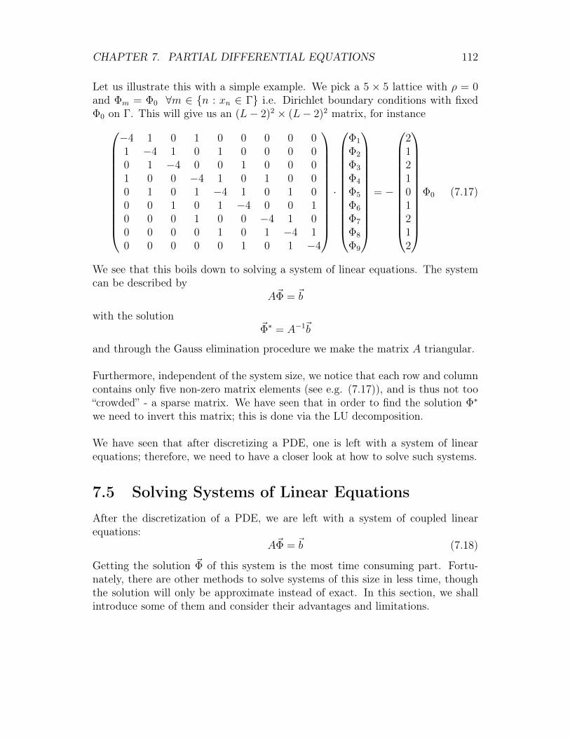
CHAPTER 7. PARTIAL DIFFERENTIAL EQUATIONS 112
Let us illustrate this with a simple example. We pick a 5 × 5 lattice with ρ = 0and Φm = Φ0 ∀m ∈ {n : xn ∈ Γ} i.e. Dirichlet boundary conditions with fixedΦ0 on Γ. This will give us an (L− 2)2 × (L− 2)2 matrix, for instance
−4 1 0 1 0 0 0 0 01 −4 1 0 1 0 0 0 00 1 −4 0 0 1 0 0 01 0 0 −4 1 0 1 0 00 1 0 1 −4 1 0 1 00 0 1 0 1 −4 0 0 10 0 0 1 0 0 −4 1 00 0 0 0 1 0 1 −4 10 0 0 0 0 1 0 1 −4
·
Φ1
Φ2
Φ3
Φ4
Φ5
Φ6
Φ7
Φ8
Φ9
= −
212101212
Φ0 (7.17)
We see that this boils down to solving a system of linear equations. The systemcan be described by
A~Φ = ~b
with the solution~Φ∗ = A−1~b
and through the Gauss elimination procedure we make the matrix A triangular.
Furthermore, independent of the system size, we notice that each row and columncontains only five non-zero matrix elements (see e.g. (7.17)), and is thus not too“crowded” - a sparse matrix. We have seen that in order to find the solution Φ∗
we need to invert this matrix; this is done via the LU decomposition.
We have seen that after discretizing a PDE, one is left with a system of linearequations; therefore, we need to have a closer look at how to solve such systems.
7.5 Solving Systems of Linear EquationsAfter the discretization of a PDE, we are left with a system of coupled linearequations:
A~Φ = ~b (7.18)
Getting the solution ~Φ of this system is the most time consuming part. Fortu-nately, there are other methods to solve systems of this size in less time, thoughthe solution will only be approximate instead of exact. In this section, we shallintroduce some of them and consider their advantages and limitations.
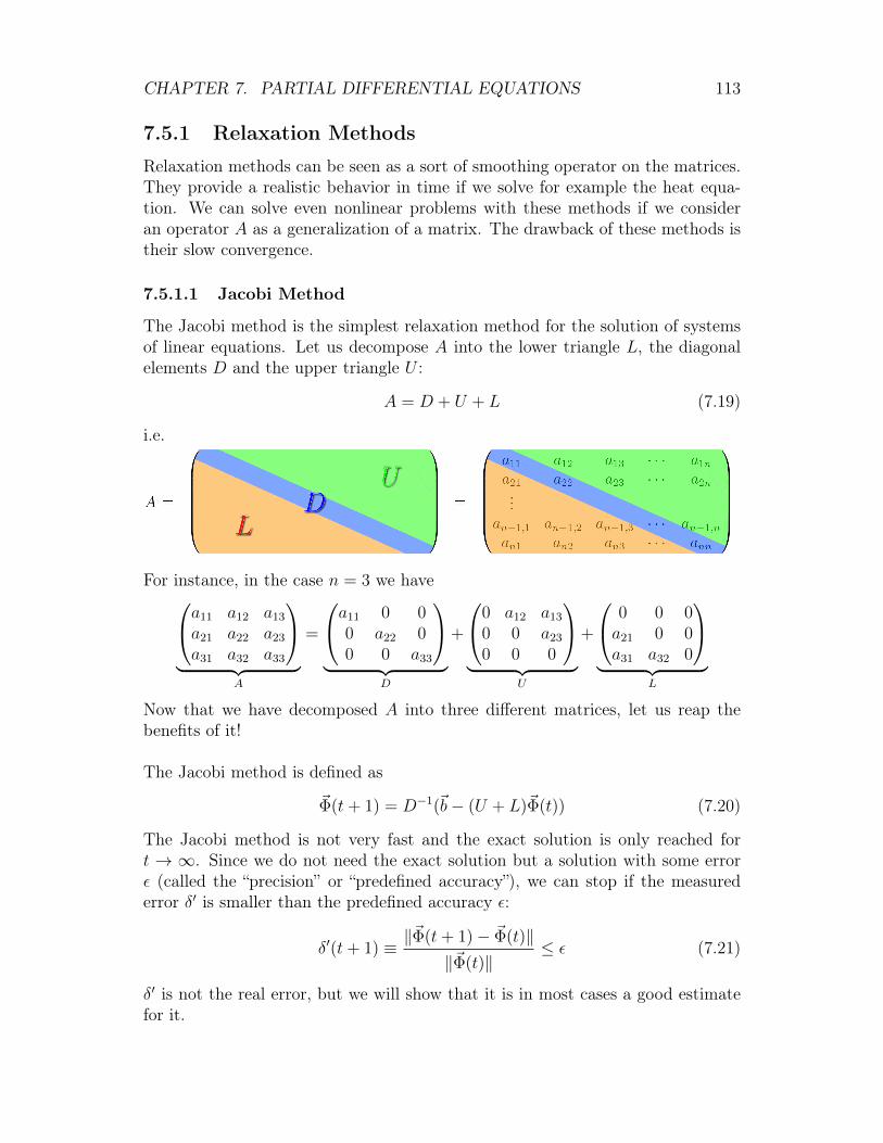
CHAPTER 7. PARTIAL DIFFERENTIAL EQUATIONS 113
7.5.1 Relaxation Methods
Relaxation methods can be seen as a sort of smoothing operator on the matrices.They provide a realistic behavior in time if we solve for example the heat equa-tion. We can solve even nonlinear problems with these methods if we consideran operator A as a generalization of a matrix. The drawback of these methods istheir slow convergence.
7.5.1.1 Jacobi Method
The Jacobi method is the simplest relaxation method for the solution of systemsof linear equations. Let us decompose A into the lower triangle L, the diagonalelements D and the upper triangle U :
A = D + U + L (7.19)
i.e.
For instance, in the case n = 3 we havea11 a12 a13
a21 a22 a23
a31 a32 a33
︸ ︷︷ ︸
A
=
a11 0 00 a22 00 0 a33
︸ ︷︷ ︸
D
+
0 a12 a13
0 0 a23
0 0 0
︸ ︷︷ ︸
U
+
0 0 0a21 0 0a31 a32 0
︸ ︷︷ ︸
L
Now that we have decomposed A into three different matrices, let us reap thebenefits of it!
The Jacobi method is defined as
~Φ(t+ 1) = D−1(~b− (U + L)~Φ(t)) (7.20)
The Jacobi method is not very fast and the exact solution is only reached fort → ∞. Since we do not need the exact solution but a solution with some errorε (called the “precision” or “predefined accuracy”), we can stop if the measurederror δ′ is smaller than the predefined accuracy ε:
δ′(t+ 1) ≡ ‖~Φ(t+ 1)− ~Φ(t)‖‖~Φ(t)‖
≤ ε (7.21)
δ′ is not the real error, but we will show that it is in most cases a good estimatefor it.
CHAPTER 7. PARTIAL DIFFERENTIAL EQUATIONS 114
Let us start out with the formal definition of the error; quite trivially, the er-ror at a given time step t is the difference between the exact solution A−1~b andthe approximate solution Φ(t) we have obtained at that time step:
~δ(t+ 1) ≡ A−1~b− ~Φ(t+ 1)
= A−1~b−D−1(AA−1)(~b− (U + L)~Φ(t))
= −D−1(U + L)(A−1~b− ~Φ(t))
= −D−1(U + L)~δ(t)
We thus see that from this simple definition (and a bit of plug and play) we havederived an expression that we can rewrite as
~δ(t+ 1) = −Λ~δ(t) (7.22)
with the evolution operator Λ of the error (note that Λ is a matrix). The evolutionoperator establishes a link between the error at one time step and the next (andconsequently between the current one and the previous one). We can simplyidentify Λ in the previous calculation and find
Λ = D−1(U + L)
After n time steps, the error will be the product of evolution operators Λ and theinitial “distance”; One can immediately draw some conclusions from this finding:
• As we want to get closer to the solution, the error has to decrease. Conse-quently, the largest eigenvalue λ of Λ needs to be smaller than one, |λ| < 1.Generally speaking, λ satisfies 0 < |λ| < 1.
• The smaller the largest absolute eigenvalue λ is, the faster the method willconverge.
If we consider enough time steps n, we may write the approximate solution as thesum of the exact solution with an error:
~Φn ≈ ~Φ∗ + λn·~c (7.23)
Of course one issue has not been addressed yet - how do we find λ in the firstplace? Given that we pick up one factor of λ at each time step, we simply thinkof λ as the ratio between two time steps and thus conclude that
‖~Φ(n+ 1)− ~Φ(n)‖‖~Φ(n)− ~Φ(n− 1)‖
≈ λn+1 − λn
λn − λn−1= λ (7.24)
CHAPTER 7. PARTIAL DIFFERENTIAL EQUATIONS 115
We have mentioned that there is a real error δ and that there is a second errorδ′ (which was defined in (7.21) ). Let us try to find a link between the two. Westart out by using the approximation (7.23) in the definition of the error:
δ(n) =||~Φ∗ − ~Φ(n)||||~Φ(n)||
(7.23)≈ ||~Φ∗ − ~Φ∗ − λn · ~c||
||~Φ(n)||=||~c||||~Φ(n)||
λn
and we can also use (7.23) to rewrite (7.21) :
δ′(n+1) ≡ ||~Φ(n+ 1)− ~Φ(n)||||~Φ(n)||
(7.23)≈ ||~Φ∗ + λn+1 · ~c− ~Φ∗ − λn · ~c||
||~Φ(n)||=||~c||||~Φ(n)||
λn︸ ︷︷ ︸δ(n)
|λ−1|
so we can link δ and δ′δ′(n+ 1) ≈ (1− λ)δ(n)
i.e.δ(n) ≈ δ′(n+ 1)
1− λor we may write
δ(n) ≈ δ′(n+ 1)
1− λ(7.21)=
(1
1− λ
)||~Φ(n+ 1)− ~Φ(n)||
||~Φ(n)||(7.25)
Of course we can rewrite 1− λ in a smart way, using (7.24):
1− λ =||~Φ(n)− ~Φ(n− 1)||||~Φ(n)− ~Φ(n− 1)||︸ ︷︷ ︸
1
− ||~Φ(n+ 1)− ~Φ(n)||||~Φ(n)− ~Φ(n− 1)||︸ ︷︷ ︸
λ
We can use this alternative way of writing 1−λ to reformulate (7.25) ; we obtain
δ(n) ≈ ||~Φ(n+ 1)− ~Φ(n)|| ||~Φ(n)− ~Φ(n− 1)||
||~Φ(n)||(||~Φ(n)− ~Φ(n− 1)|| − ||~Φ(n+ 1)− ~Φ(n)||
) (7.26)
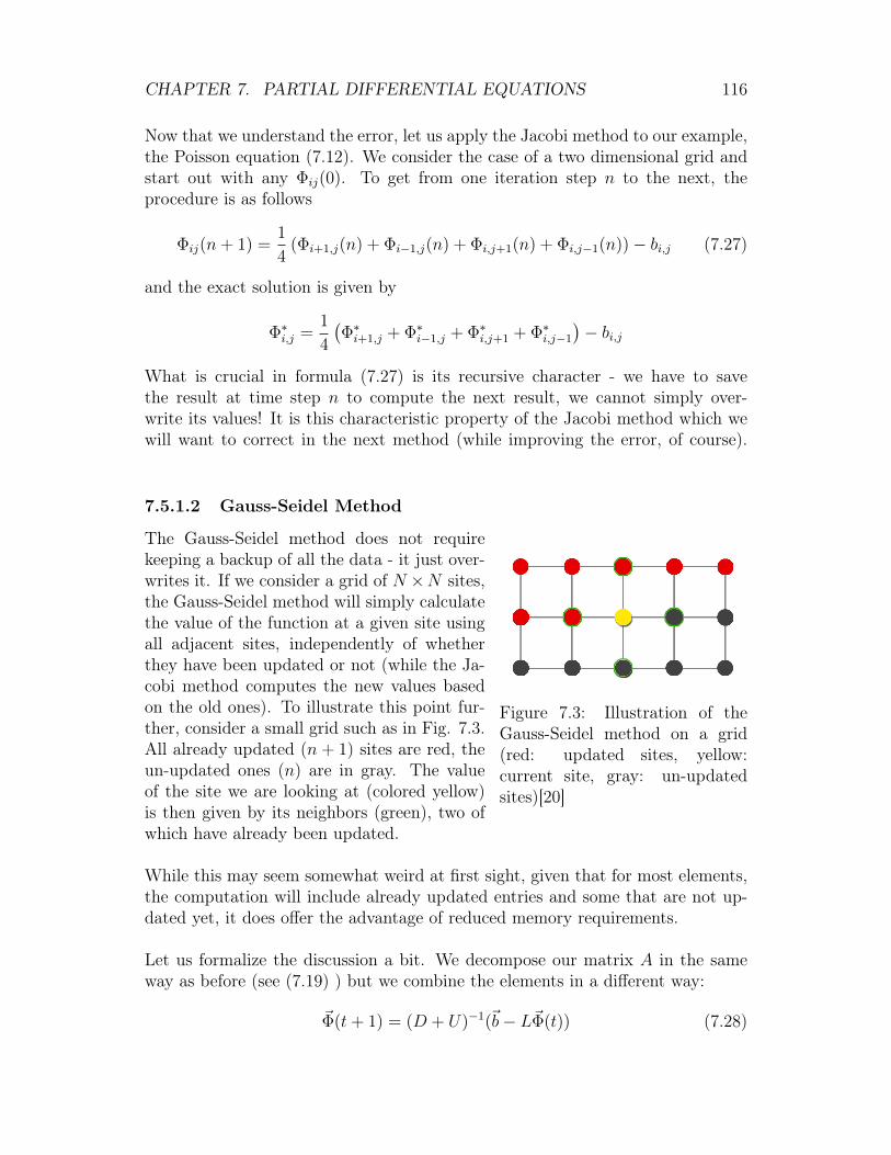
CHAPTER 7. PARTIAL DIFFERENTIAL EQUATIONS 116
Now that we understand the error, let us apply the Jacobi method to our example,the Poisson equation (7.12). We consider the case of a two dimensional grid andstart out with any Φij(0). To get from one iteration step n to the next, theprocedure is as follows
Φij(n+ 1) =1
4(Φi+1,j(n) + Φi−1,j(n) + Φi,j+1(n) + Φi,j−1(n))− bi,j (7.27)
and the exact solution is given by
Φ∗i,j =1
4
(Φ∗i+1,j + Φ∗i−1,j + Φ∗i,j+1 + Φ∗i,j−1
)− bi,j
What is crucial in formula (7.27) is its recursive character - we have to savethe result at time step n to compute the next result, we cannot simply over-write its values! It is this characteristic property of the Jacobi method which wewill want to correct in the next method (while improving the error, of course).
Figure 7.3: Illustration of theGauss-Seidel method on a grid(red: updated sites, yellow:current site, gray: un-updatedsites)[20]
7.5.1.2 Gauss-Seidel Method
The Gauss-Seidel method does not requirekeeping a backup of all the data - it just over-writes it. If we consider a grid of N ×N sites,the Gauss-Seidel method will simply calculatethe value of the function at a given site usingall adjacent sites, independently of whetherthey have been updated or not (while the Ja-cobi method computes the new values basedon the old ones). To illustrate this point fur-ther, consider a small grid such as in Fig. 7.3.All already updated (n + 1) sites are red, theun-updated ones (n) are in gray. The valueof the site we are looking at (colored yellow)is then given by its neighbors (green), two ofwhich have already been updated.
While this may seem somewhat weird at first sight, given that for most elements,the computation will include already updated entries and some that are not up-dated yet, it does offer the advantage of reduced memory requirements.
Let us formalize the discussion a bit. We decompose our matrix A in the sameway as before (see (7.19) ) but we combine the elements in a different way:
~Φ(t+ 1) = (D + U)−1(~b− L~Φ(t)) (7.28)
CHAPTER 7. PARTIAL DIFFERENTIAL EQUATIONS 117
When we look at the error (and carry out the same calculation as for the Jacobimethod) we find that the error evolution operator is given by
Λ = (D + U)−1L
while the stopping criteria is
δ(t) =‖~Φ(t+ 1)− ~Φ(t)‖
(1− λ)‖~Φ(t)‖≤ ε
Of course we immediately notice that Λ has changed. Most importantly, we seethat the denominator has become (D+U) instead of D, making the largest eigen-value λmax of Λ smaller, consequently decreasing the error at each time step andincreasing the convergence speed of the method.
In a nutshell: We have found a method that not only reduces memory require-ments (by eliminating the need for a backup) but also converges faster. How canwe improve this further?
7.5.1.3 Successive Over-Relaxation (SOR) Method
The successive over-relaxation (SOR) method is a simple generalization of Gauss-Seidel; it tries to improve the convergence of the Gauss-Seidel relaxation methodby introducing an over-relaxation parameter ω:
~Φ(t+ 1) = (D + ωU)−1(ω~b+ [(1− ω)D − ωL]~Φ(t)
)(7.29)
Thanks to the introduction of ω, the denominator in Λ becomes even larger, per-mitting faster convergence. However, if we push this too far (ω > 2), the algorithmwill become unstable (and the solution will blow up).
If we set ω = 1, we are back at the Gauss-Seidel method. Typically, ω is setto a value between 1 and 2 and has to be determined by trial and error.
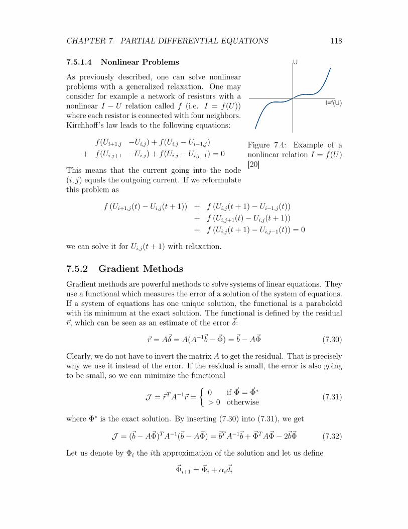
CHAPTER 7. PARTIAL DIFFERENTIAL EQUATIONS 118
7.5.1.4 Nonlinear Problems
Figure 7.4: Example of anonlinear relation I = f(U)[20]
As previously described, one can solve nonlinearproblems with a generalized relaxation. One mayconsider for example a network of resistors with anonlinear I − U relation called f (i.e. I = f(U))where each resistor is connected with four neighbors.Kirchhoff’s law leads to the following equations:
f(Ui+1,j −Ui,j) + f(Ui,j − Ui−1,j)
+ f(Ui,j+1 −Ui,j) + f(Ui,j − Ui,j−1) = 0
This means that the current going into the node(i, j) equals the outgoing current. If we reformulatethis problem as
f (Ui+1,j(t)− Ui,j(t+ 1)) + f (Ui,j(t+ 1)− Ui−1,j(t))
+ f (Ui,j+1(t)− Ui,j(t+ 1))
+ f (Ui,j(t+ 1)− Ui,j−1(t)) = 0
we can solve it for Ui,j(t+ 1) with relaxation.
7.5.2 Gradient Methods
Gradient methods are powerful methods to solve systems of linear equations. Theyuse a functional which measures the error of a solution of the system of equations.If a system of equations has one unique solution, the functional is a paraboloidwith its minimum at the exact solution. The functional is defined by the residual~r, which can be seen as an estimate of the error ~δ:
~r = A~δ = A(A−1~b− ~Φ) = ~b− A~Φ (7.30)
Clearly, we do not have to invert the matrix A to get the residual. That is preciselywhy we use it instead of the error. If the residual is small, the error is also goingto be small, so we can minimize the functional
J = ~rTA−1~r =
{0 if ~Φ = ~Φ∗
> 0 otherwise(7.31)
where Φ∗ is the exact solution. By inserting (7.30) into (7.31), we get
J = (~b− A~Φ)TA−1(~b− A~Φ) = ~bTA−1~b+ ~ΦTA~Φ− 2~b~Φ (7.32)
Let us denote by Φi the ith approximation of the solution and let us define
~Φi+1 = ~Φi + αi~di

CHAPTER 7. PARTIAL DIFFERENTIAL EQUATIONS 119
with ~Φi being the start value or the value of the last iteration, ~di the direction ofthe step and αi the step length. If we insert this into (7.32), we obtain
J = ~bTA−1~b+ ~ΦTi A~Φi + 2αi~d
Ti A~Φi + α2
i~dTi A
~di − 2~bT ~Φi − 2αi~bT ~di
If we minimize the functional J along the lines given by ~d, we will find the bestvalue for α at which J is minimal: α. The condition is obviously
∂J∂αi
= 2~dti
(αiA~di − ~ri
)!
= 0
from which we can conclude that the optimal value is given by
αi =~dti~ri~dtiA
~di
Of course αi is to be calculated for each step. The most difficult part of thegradient methods is the computation of the direction of the step. Consequently,gradient methods are classified by this feature.
7.5.2.1 Steepest Descent
The most intuitive method of getting the direction is to choose the direction withthe largest (negative) gradient. As an analogy, one can think of standing on amountain top and trying to get down to the valley the quickest way possible, notnecessarily the most comfortable way. One would intuitively choose the steepestpossible direction. In the case of the steepest descent method, the direction isgiven by the residual at the point we have reached:
~di = ~ri (7.33)
Figure 7.5: An illustra-tion of the gradient de-scent method on an irregu-lar paraboloid. One clearlysees the “zig-zagging” na-ture. [14]
However, the steepest descent method has amajor disadvantage which is that it does nottake the optimal direction if the functional isnot a regular paraboloid. It is a constant“swing and miss” situation as for instance inFig. 7.5 where the method does lead us tothe exact solution in the center, but takes along time to do so as it keeps changing direc-tion.
The steepest descent algorithm is as follows:
1. Start with ~Φi and choose
~di = ~ri = ~b− A~Φi
CHAPTER 7. PARTIAL DIFFERENTIAL EQUATIONS 120
2. Evaluate~ui = A~ri
and store the result (we need it twice). Calculate the length of the step:
αi =~r2i
~ri~ui
3. Advance αi in the direction of ~di (which is the same as ~ri) and compute thevalue of the function at this point:
~Φi+1 = ~Φi + αi~ri
4. Update the residual for the next step:
~ri+1 = ~ri − αi~ui
5. Repeat steps 2 to 4 until the residual is sufficiently small.
The vector ~ui is the temporary stored product A~ri so that we need to computeit only once per step since this is the most time consuming part of the algorithmand scales with N2, where N is the number of equations to be solved. If A issparse, this matrix-vector product is of order N .
While this method is already very promising, we still want to improve it as thesituation as in Fig. 7.5 is somewhat unsettling and inefficient.
7.5.2.2 Conjugate Gradient
We fix the previously observed behavior in the so-called conjugate gradient method.This method takes the functional and deforms it in such a way that it looks like aregular paraboloid - it is only then that it carries out the steepest descent method.In this way, we avoid the behavior we saw previously as we get to root of the prob-lem and get rid of irregular paraboloids.
This can be achieved if we take the new direction conjugate to all previous onesusing the Gram-Schmidt orthogonalization process:
~di = ~ri −i−1∑j=1
~d Tj A~ri~d Tj A
~dj
~dj (7.34)
Then, all directions ~di are conjugate to each other (with respect to A acting as a“metric”):
~d Ti A~dj = δij
CHAPTER 7. PARTIAL DIFFERENTIAL EQUATIONS 121
It needs to be noted at this point that the conjugate gradient method, and gradientmethods in general, are only a valuable option for positive definite and symmetricmatrices A.
The algorithm is as follows:
1. Initialize with some vector ~Φ1 and compute the first residual. Then, takethe residual as the direction of your first step:
~r1 = ~b− A~Φ1, ~d1 = ~r1
2. Compute the temporary scalar
c = (~d Ti A~di)−1
Note: There is no need for an inversion of the matrix A for this, as wefirst compute the scalar product which leads to a scalar. However, we needto compute a matrix-vector product, which is of complexity N2 for densematrices and N for sparse matrices.
3. Compute the length of the step:
αi = c~riT ~di
4. Carry out the step:~Φi+1 = ~Φi + αi~di
If the residual is sufficiently small, e.g. ~r Ti ~ri < ε (where ε is the predefinedprecision), we can stop.
5. Update the residual for the error estimation and for the next step:
~ri+1 = ~b− A~Φi+1
6. Compute the direction of the next step:
~di+1 = ~ri+1 − (c~r Ti+1A~di)~di
7. Repeat steps 2 to 6.
CHAPTER 7. PARTIAL DIFFERENTIAL EQUATIONS 122
7.5.2.3 Biconjugate gradient
If we are dealing with a matrix that does not fulfill our requirements of a symmetricand positive definite matrix, we are somewhat outside the possibilities of theconjugate gradient method. Interestingly, we can adapt the gradient method tocontain two residuals (hence “biconjugate” gradient method) and the procedurethen works beautifully. The residuals are
~r = ~b− A~Φ and ~r = ~b− AT ~Φ
However, this method does not always converge and can become unstable. Theprocedure is as follows:
1. Initialize:~r1 = ~b− A~Φ , ~d1 = ~r1
~r1 = ~b− At~Φ , ~d1 = ~r1
2. Iterate:
~ri+1 = ~ri − αiA~di , ~ri+1 = ~ri − αiAT ~di , α = c~rTi ~ri~di+1 = ~ri + αi~di , ~di+1 = ~ri + αi~di , α = c~rTi ~ri
with c = (~dTi A~di)−1 and c = ( ~dTi A
~di)−1
3. Stop as soon as
~r Ti ~ri < ε ⇒ ~Φn = ~Φ1 +n∑i
αi~di
7.5.3 Preconditioning
When using one of the previous methods to solve a system of linear equations, onemay notice poor performance because the methods converge very slowly. Thisis the case if the matrix is badly conditioned: The diagonal elements are almostequal to the sum of the other elements on their row. The solution to this problemis called preconditioning.
The idea is simple: We find a matrix P−1 which is cheap to compute and de-livers a good approximation of the inverse of the matrix of our problem. (whilethe idea is simple, the process of finding such a matrix is really not!). We thensolve the preconditioned system obtained by a multiplication from the left:(
P−1A)~Φ = P−1~b (7.35)
CHAPTER 7. PARTIAL DIFFERENTIAL EQUATIONS 123
7.5.3.1 Jacobi Preconditioner
Let us consider a first preconditioner, the Jacobi preconditioner. Its name hintsat the fact that it shares a core ingredient with the Jacobi method (a member ofthe group of splitting methods1) where we pick the diagonal entries (i.e. in ournotation from (7.19), P = D). This choice is shared by the Jacobi preconditioner,where we also use the diagonal entries:
Pij = Aijδij =
{Aii if i = j0 otherwise
We then invert the obtained diagonal matrix:
P−1ij = δij
1
Aii(7.36)
7.5.3.2 SOR Preconditioner
Another example of a preconditioner is the SOR preconditioner:
P =
(D
ω+ L
)−1ω
2− ωD−1
(D
ω+ U
)(7.37)
where ω is the relaxation parameter, 0 ≤ ω < 2. For symmetric matrices withU = LT , the method is called Symmetric Successive Over-Relaxation or SSOR,in which
P =
(D
ω+ L
)−1ω
2− ωD−1
(D
ω+ LT
)
1The group of splitting methods follows the scheme
Ax = b ⇒ 0 = −Ax+ b ⇒ 0 = −(A+ P − P )x+ b
soPx = (P −A)x+ b
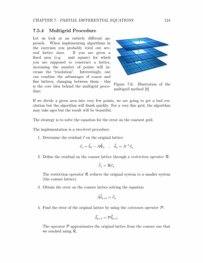
CHAPTER 7. PARTIAL DIFFERENTIAL EQUATIONS 124
7.5.4 Multigrid Procedure
Figure 7.6: Illustration of themultigrid method [8]
Let us look at an entirely different ap-proach. When implementing algorithms inthe exercises you probably tried out sev-eral lattice sizes. If you are given afixed area (e.g. unit square) for whichyou are supposed to construct a lattice,increasing the number of points will in-crease the “resolution”. Interestingly, onecan combine the advantages of coarse andfine lattices, changing between them - thisis the core idea behind the multigrid proce-dure.
If we divide a given area into very few points, we are going to get a bad res-olution but the algorithm will finish quickly. For a very fine grid, the algorithmmay take ages but the result will be beautiful.
The strategy is to solve the equation for the error on the coarsest grid.
The implementation is a two-level procedure:
1. Determine the residual ~r on the original lattice:
~rn = ~bn − A~Φn , ~δn = A−1~rn
2. Define the residual on the coarser lattice through a restriction operator R:
~rn = R~rn
The restriction operator R reduces the original system to a smaller system(the coarser lattice).
3. Obtain the error on the coarser lattice solving the equation
A~δn+1 = ~rn
4. Find the error of the original lattice by using the extension operator P :
~δn+1 = P~δn+1
The operator P approximates the original lattice from the coarser one thatwe reached using R.
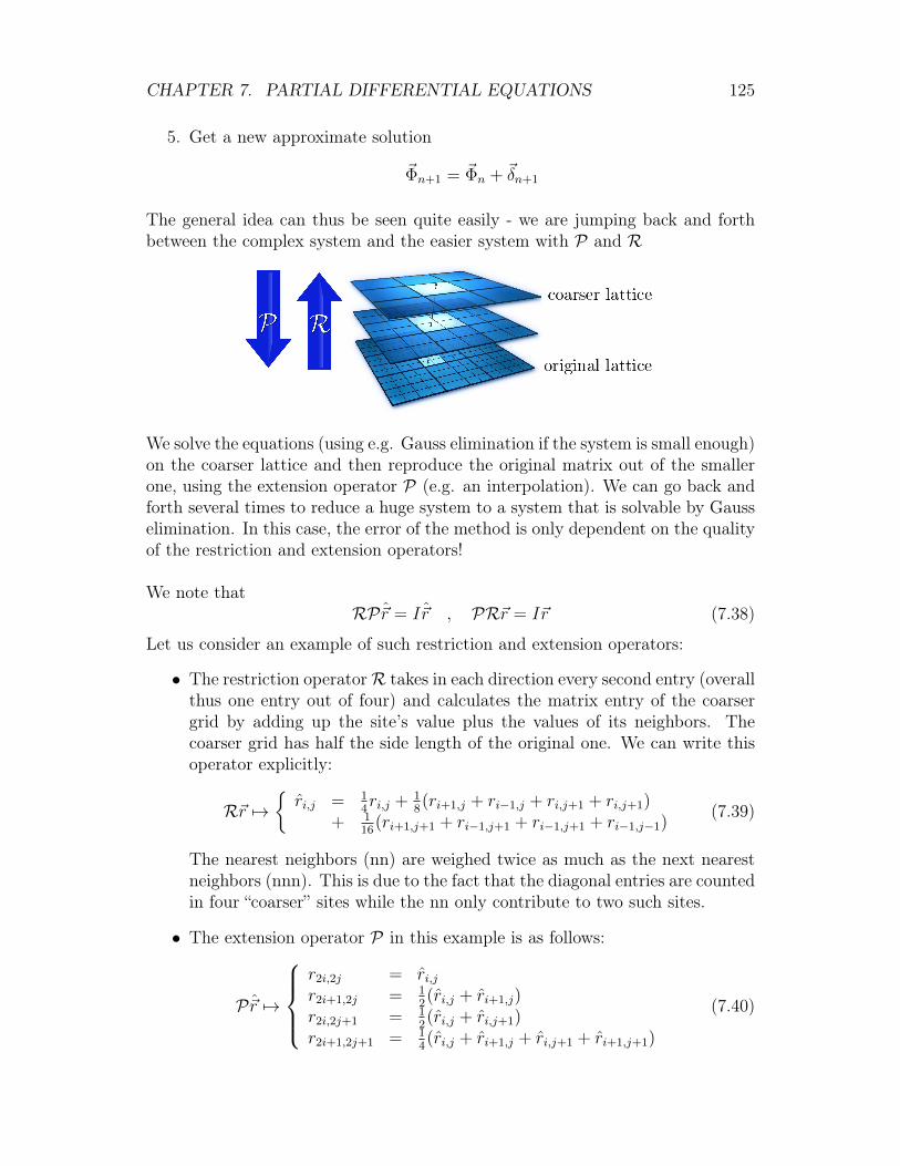
CHAPTER 7. PARTIAL DIFFERENTIAL EQUATIONS 125
5. Get a new approximate solution
~Φn+1 = ~Φn + ~δn+1
The general idea can thus be seen quite easily - we are jumping back and forthbetween the complex system and the easier system with P and R
We solve the equations (using e.g. Gauss elimination if the system is small enough)on the coarser lattice and then reproduce the original matrix out of the smallerone, using the extension operator P (e.g. an interpolation). We can go back andforth several times to reduce a huge system to a system that is solvable by Gausselimination. In this case, the error of the method is only dependent on the qualityof the restriction and extension operators!
We note thatRP~r = I~r , PR~r = I~r (7.38)
Let us consider an example of such restriction and extension operators:
• The restriction operatorR takes in each direction every second entry (overallthus one entry out of four) and calculates the matrix entry of the coarsergrid by adding up the site’s value plus the values of its neighbors. Thecoarser grid has half the side length of the original one. We can write thisoperator explicitly:
R~r 7→{ri,j = 1
4ri,j + 1
8(ri+1,j + ri−1,j + ri,j+1 + ri,j+1)
+ 116
(ri+1,j+1 + ri−1,j+1 + ri−1,j+1 + ri−1,j−1)(7.39)
The nearest neighbors (nn) are weighed twice as much as the next nearestneighbors (nnn). This is due to the fact that the diagonal entries are countedin four “coarser” sites while the nn only contribute to two such sites.
• The extension operator P in this example is as follows:
P~r 7→
r2i,2j = ri,jr2i+1,2j = 1
2(ri,j + ri+1,j)
r2i,2j+1 = 12(ri,j + ri,j+1)
r2i+1,2j+1 = 14(ri,j + ri+1,j + ri,j+1 + ri+1,j+1)
(7.40)
CHAPTER 7. PARTIAL DIFFERENTIAL EQUATIONS 126
The operators P and R fulfill one rather interesting condition, but to be ableto stomach it well we need to first talk about function spaces. Let us pick anyfunction living on the original grid and denote it by u(x, y). Obviously, a functionliving on the original grid will take its arguments from the original grid so thearguments are x and y (i.e. the coordinates of the original grid).If we pick a second function living on the coarser grid and denote it by v(x, y)(using ˆ to refer to elements on the coarser grid), we see that it will take itsarguments from coordinates of the coarser grid, i.e. x, y and not from the originalgrid (i.e. x, y).While we already know that we can change between the coarser grid and theoriginal grid with R and P , there is a special relation that applies to functionsliving on these two grids: If we consider two functions u(x, y) (on the original grid)and v(x, y) (on the coarser grid)as introduced, we can show with a given scalarproduct that the extension operator and the restriction operator are adjoint:∑
x,y
P v(x, y) · u(x, y) = h2∑x,y
v(x, y) · Ru(x, y)
Here, h denotes the scaling factor of the finer matrix to the coarser matrix whichis given by the coefficient of the respective number of rows. In our example h is2.
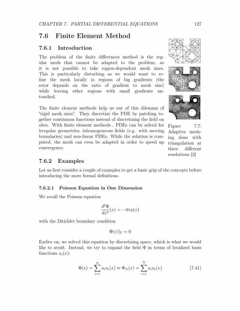
CHAPTER 7. PARTIAL DIFFERENTIAL EQUATIONS 127
7.6 Finite Element Method
7.6.1 Introduction
Figure 7.7:Adaptive mesh-ing done withtriangulation atthree differentresolutions [2]
The problem of the finite differences method is the reg-ular mesh that cannot be adapted to the problem, soit is not possible to take region-dependent mesh sizes.This is particularly disturbing as we would want to re-fine the mesh locally in regions of big gradients (theerror depends on the ratio of gradient to mesh size)while leaving other regions with small gradients un-touched.
The finite element methods help us out of this dilemma of“rigid mesh sizes”. They discretize the PDE by patching to-gether continuous functions instead of discretizing the field onsites. With finite element methods , PDEs can be solved forirregular geometries, inhomogeneous fields (e.g. with movingboundaries) and non-linear PDEs. While the solution is com-puted, the mesh can even be adapted in order to speed upconvergence.
7.6.2 Examples
Let us first consider a couple of examples to get a basic grip of the concepts beforeintroducing the more formal definitions.
7.6.2.1 Poisson Equation in One Dimension
We recall the Poisson equation
d2Φ
dx2(x) = −4πρ(x)
with the Dirichlet boundary condition
Φ(x)|Γ = 0
Earlier on, we solved this equation by discretizing space, which is what we wouldlike to avoid. Instead, we try to expand the field Φ in terms of localized basisfunctions ui(x):
Φ(x) =∞∑i=1
aiui(x) ≈ ΦN(x) =N∑i=1
aiui(x) (7.41)
CHAPTER 7. PARTIAL DIFFERENTIAL EQUATIONS 128
We approximate the exact solution Φ(x) with ΦN(x), which is the superpositionof a finite number of basis functions (instead of an infinite number as in the exactsolution). Each basis function has a coefficient ai. We can obtain the expansioncoefficients ai from (7.41) by introducing so-called “weight functions” wj(x):
−N∑i=1
ˆ L
0
aid2uidx2
(x)wj(x)dx = 4π
ˆ L
0
ρ(x)wj(x)dx , j ∈ {1, ..., N} (7.42)
The simplest case is the so-called Galerkin method where we simply pick theweight functions to be the basis functions, i.e. wj(x) = uj(x).
We find N coupled equations. When we go from derivatives of Φ to derivatives ofuj, we do not have to find the derivatives numerically (for a sensibly chosen basisof functions), which significantly simplifies the problem. When we separate andinsert, we obtain
A~a = ~b (7.43)
where ~a is the N -dimensional vector whose entries are the expansion coefficientsfrom (7.41). Let us now try to find an explicit expression for the matrix andvector entries, for which we go back to (7.42):
N∑i=1
ai
(−ˆ L
0
d2uidx2
(x)wj(x)dx
)︸ ︷︷ ︸
Aij
= 4π
ˆ L
0
ρ(x)wj(x)dx︸ ︷︷ ︸bj
, j ∈ {1, ..., N}
so the matrix element is given by
Aij = −ˆ L
0
u′′
i (x)wj(x)dxP.I.=
ˆ L
0
u′
i(x)w′
j(x)dx
where we have used partial integration, and the vector bj can be read off as
bj(x) = 4π
ˆ L
0
ρ(x)wj(x)dx (7.44)
As a side comment, if we use hat functions as a basis, we obtain matrix elementsAij that look like the discrete elements. We have been talking a lot about basisfunctions so far, so let us consider an example of basis functions.
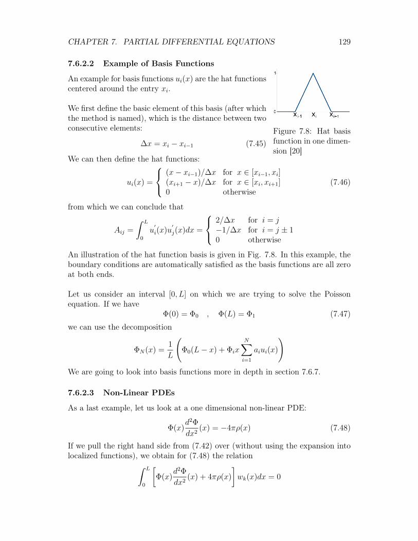
CHAPTER 7. PARTIAL DIFFERENTIAL EQUATIONS 129
7.6.2.2 Example of Basis Functions
Figure 7.8: Hat basisfunction in one dimen-sion [20]
An example for basis functions ui(x) are the hat functionscentered around the entry xi.
We first define the basic element of this basis (after whichthe method is named), which is the distance between twoconsecutive elements:
∆x = xi − xi−1 (7.45)
We can then define the hat functions:
ui(x) =
(x− xi−1)/∆x for x ∈ [xi−1, xi](xi+1 − x)/∆x for x ∈ [xi, xi+1]0 otherwise
(7.46)
from which we can conclude that
Aij =
ˆ L
0
u′
i(x)u′
j(x)dx =
2/∆x for i = j−1/∆x for i = j ± 10 otherwise
An illustration of the hat function basis is given in Fig. 7.8. In this example, theboundary conditions are automatically satisfied as the basis functions are all zeroat both ends.
Let us consider an interval [0, L] on which we are trying to solve the Poissonequation. If we have
Φ(0) = Φ0 , Φ(L) = Φ1 (7.47)
we can use the decomposition
ΦN(x) =1
L
(Φ0(L− x) + Φix
N∑i=1
aiui(x)
)We are going to look into basis functions more in depth in section 7.6.7.
7.6.2.3 Non-Linear PDEs
As a last example, let us look at a one dimensional non-linear PDE:
Φ(x)d2Φ
dx2(x) = −4πρ(x) (7.48)
If we pull the right hand side from (7.42) over (without using the expansion intolocalized functions), we obtain for (7.48) the relation
ˆ L
0
[Φ(x)
d2Φ
dx2(x) + 4πρ(x)
]wk(x)dx = 0
CHAPTER 7. PARTIAL DIFFERENTIAL EQUATIONS 130
which we have to solve. This is approximately equivalent to the coupled non-linearsystem of equations given by
∑i,j
Aijkaiaj = bk with Aijk = −ˆ L
0
ui(x)u′′
j (x)wk(x)dx
We may solve such a system using the Picard iteration:
Picard Iteration
The Picard iteration consists of three simple steps:
• Start with a guess for Φ0
• Solve the linear equation for Φ:
Φ0(x)d2Φ1
dx2(x) = −4πρ(x)
• Iterate:Φn(x)
d2Φn+1
dx2(x) = −4πρ(x)
7.6.3 Function on Element
We have so far only considered one dimension; to be useful in practice, we needto go to at least two dimensions (if not more). In two dimensions, we define thefunction over one element, which is a triangle of the triangulation.
One possible approach is linearization
Φ(~r) ≈ c1 + c2x+ c3y
or approximation by a paraboloid
Φ(~r) ≈ c1 + c2x+ c3y + c4x2 + c5xy + c6y
2
In the case of the paraboloid fit, we can have smooth transitions between elements(which is not possible for the linear fit for non-trivial cases).
7.6.4 Variational Approach
The basic idea behind the variational approach is the minimization of the function
E =
ˆ ˆG
(1
2(∇Φ)2 +
1
2aΦ2 + bΦ
)dxdy +
ˆΓ
(α2
Φ2 + βΦ)ds
CHAPTER 7. PARTIAL DIFFERENTIAL EQUATIONS 131
where we have split up the functional into a volume contribution and a surfacecontribution (represented by the integral over G and Γ, respectively). This defi-nition of E will be motivated later on.
The first step towards minimization of the functional is the determination of itsvariation δE:
δE =
ˆ ˆG
(∇Φδ∇Φ + aΦδΦ + bδΦ) dxdy +
ˆΓ
(aΦδΦ + βδΦ) ds
We recall Green’s theorem from calculusˆ ˆG
∇u∇vdxdy = −ˆ ˆ
G
v∆udxdy +
ˆΓ
∂u
∂nvds
Of course we can use Green’s theorem to modify the first term in δE (both u andv can be identified with Φ). We obtain
δE =
ˆ ˆG
(−∆Φ + aΦ + b) δΦdxdy +
ˆΓ
(aΦ + β +
∂Φ
∂n
)δΦds = 0
We immediately recognize two different cases for a and b in ∆Φ = aΦ + b:
• If we set a = 0, we obtain the Poisson equation (∆Φ = b with b = −4πρ)
• If we set b = 0, we obtain the Helmholtz equation (∆Φ = aΦ with a = k2)
We consider the first term of the total energy
E =∑
elements j
ˆ ˆGj
((∇Φ)2 + aΦ2 + bΦ
)dxdy
which can rewrite asE = ~ΦtA~Φ +~b · ~Φ
Minimizing yields∂E
∂Φ= 0 ⇒ A~Φ +~b = 0 (7.49)
We are going to come back to this equation in sections 7.6.8 and 7.6.9.
7.6.5 Standard Form
We can transform any element j into the standard form. In two dimensions wehave
x = x1 + (x2 − x1)ξ + (x3 − x1)η
y = y1 + (y2 − y1)ξ + (y3 − y1)η
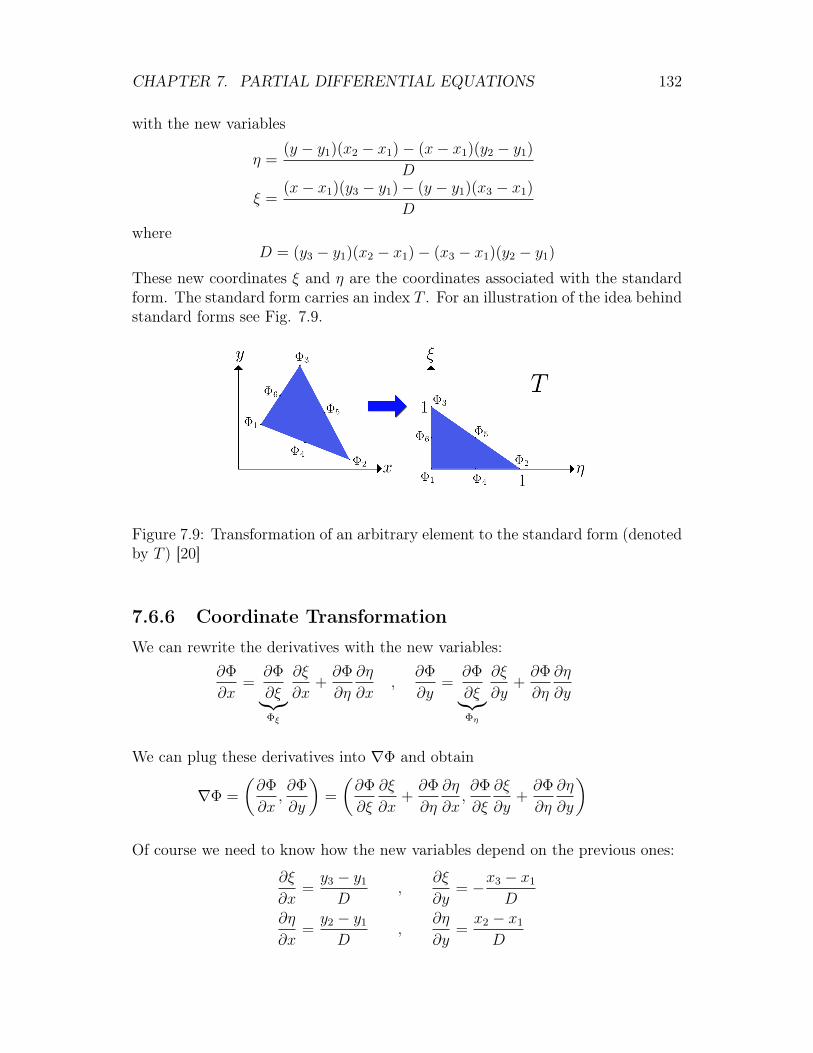
CHAPTER 7. PARTIAL DIFFERENTIAL EQUATIONS 132
with the new variables
η =(y − y1)(x2 − x1)− (x− x1)(y2 − y1)
D
ξ =(x− x1)(y3 − y1)− (y − y1)(x3 − x1)
D
whereD = (y3 − y1)(x2 − x1)− (x3 − x1)(y2 − y1)
These new coordinates ξ and η are the coordinates associated with the standardform. The standard form carries an index T . For an illustration of the idea behindstandard forms see Fig. 7.9.
Figure 7.9: Transformation of an arbitrary element to the standard form (denotedby T ) [20]
7.6.6 Coordinate Transformation
We can rewrite the derivatives with the new variables:∂Φ
∂x=
∂Φ
∂ξ︸︷︷︸Φξ
∂ξ
∂x+∂Φ
∂η
∂η
∂x,
∂Φ
∂y=
∂Φ
∂ξ︸︷︷︸Φη
∂ξ
∂y+∂Φ
∂η
∂η
∂y
We can plug these derivatives into ∇Φ and obtain
∇Φ =
(∂Φ
∂x,∂Φ
∂y
)=
(∂Φ
∂ξ
∂ξ
∂x+∂Φ
∂η
∂η
∂x,∂Φ
∂ξ
∂ξ
∂y+∂Φ
∂η
∂η
∂y
)
Of course we need to know how the new variables depend on the previous ones:
∂ξ
∂x=y3 − y1
D,
∂ξ
∂y= −x3 − x1
D∂η
∂x=y2 − y1
D,
∂η
∂y=x2 − x1
D

CHAPTER 7. PARTIAL DIFFERENTIAL EQUATIONS 133
If we would like to know |∇Φ|2 we need to know (∂Φ∂x
)2 and (∂Φ∂y
)2. Of course, theseare simply a combination of our previous results:(
∂Φ
∂x
)2
=
(∂Φ
∂ξ
∂ξ
∂x+∂Φ
∂η
∂η
∂x
)2
=(y3 − y1)2
D2Φ2ξ − 2
(y3 − y1)(y2 − y1)
D2ΦξΦη +
(y2 − y1)2
D2Φ2η(
∂Φ
∂y
)2
=
(∂Φ
∂ξ
∂ξ
∂y+∂Φ
∂η
∂η
∂y
)2
=(x3 − x1)2
D2Φ2ξ − 2
(x3 − x1)(x2 − x1)
D2ΦξΦη +
(x2 − x1)2
D2Φ2η
where we have used the notation
Φξ =∂Φ
∂ξ, Φη =
∂Φ
∂η
With these results, we know how to deal with derivatives. However, if we wouldlike to use the new coordinates for integrals, we also have to compute the Jacobimatrix
J =
(∂x∂ξ
∂x∂η
∂y∂ξ
∂y∂η
)with determinant
det(J) =∂x
∂ξ
∂y
∂η− ∂x
∂η
∂y
∂ξ= (x2 − x1)(y3 − y1)− (x3 − x1)(y2 − y1) = D
We also have to transform the integration area; let us call the transformed inte-gration area T . With this transformation, we have all ingredients to carry out theintegration with the new variables:ˆ ˆ
Gj
f(x, y)dxdy =
ˆ ˆT
f(ξ, η)det(J)dξdη
Let us now apply this to the example at hand instead of a general function f(x, y):ˆ ˆ
Gj
(Φ2x + Φ2
y
)dxdy =
ˆ ˆT
(c1Φ2
ξ + 2c2ΦξΦη + c3Φ2η
)dηdξ (7.50)
The coefficients are only calculated once for each element:
c1 =(y3 − y1)2
D+
(x3 − x1)2
D
c2 = 2(y3 − y1)(y2 − y1)
D+ 2
(x3 − x1)(x2 − x1)
D(7.51)
c3 =(y2 − y1)2
D+
(x2 − x1)2
D
CHAPTER 7. PARTIAL DIFFERENTIAL EQUATIONS 134
7.6.7 Basis functions
The discretization in the finite elements method is done by selecting basis func-tions. As we have seen in the introductory example, the exact solution Φ of a PDEcan always be written as a linear combination of infinitly many basis functions:
Φ(x) =∞∑i=1
aiui(x)
with the basis functions ui and their coefficients ai. However, the computer neitherhas infinite memory nor infinite computing speed, so we have to select a finitenumber of basis functions:
ΦN(x) =N∑i=1
aiui(x)
The basis functions ui are known and defined for all elements, so we only have tocompute their coefficients ai.
In the one-dimensional case, the linear basis functions are hat functions (as inthe introductory example in 7.6.2.2); these are 1 on the element on which theyare defined and 0 on every other element.
A clearer example is the two-dimensional case, where we divide the domain intotriangles (same size not required). As we have seen in the previous sections, thesetriangles can be transformed back to the so called standard element, whose cor-ners are located at (0,0), (0,1) and (1,0). The basis functions are defined on thistriangle and then transformed back to the original triangle for computation (seeprevious section on coordinate transformation).
Let us start out by defining the basis functions on the standard element. Inthe linear case, each basis function has value 1 in one corner and value 0 in theother two. We can thus think of the following three basis functions:
N1 = 1− ξ − ηN2 = ξ
N3 = η
where we have used the previously mentioned convention that the axes are calledξ and η to distinguish them from the axes of the original triangle (with axes xand y). A graphical representation of the linear basis functions is given in Fig.7.10.
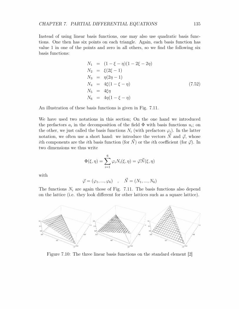
CHAPTER 7. PARTIAL DIFFERENTIAL EQUATIONS 135
Instead of using linear basis functions, one may also use quadratic basis func-tions. One then has six points on each triangle. Again, each basis function hasvalue 1 in one of the points and zero in all others, so we find the following sixbasis functions:
N1 = (1− ξ − η)(1− 2ξ − 2η)
N2 = ξ(2ξ − 1)
N3 = η(2η − 1)
N4 = 4ξ(1− ξ − η) (7.52)N5 = 4ξη
N6 = 4η(1− ξ − η)
An illustration of these basis functions is given in Fig. 7.11.
We have used two notations in this section; On the one hand we introducedthe prefactors ai in the decomposition of the field Φ with basis functions ui; onthe other, we just called the basis functions Ni (with prefactors ϕi). In the latternotation, we often use a short hand: we introduce the vectors ~N and ~ϕ, whoseith components are the ith basis function (for ~N) or the ith coefficient (for ~ϕ). Intwo dimensions we thus write
Φ(ξ, η) =6∑i=1
ϕiNi(ξ, η) = ~ϕ ~N(ξ, η)
with~ϕ = (ϕ1, ..., ϕ6) , ~N = (N1, ..., N6)
The functions Ni are again those of Fig. 7.11. The basis functions also dependon the lattice (i.e. they look different for other lattices such as a square lattice).
Figure 7.10: The three linear basis functions on the standard element [2]
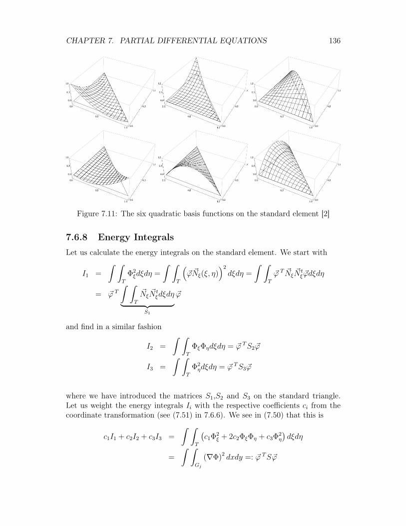
CHAPTER 7. PARTIAL DIFFERENTIAL EQUATIONS 136
Figure 7.11: The six quadratic basis functions on the standard element [2]
7.6.8 Energy Integrals
Let us calculate the energy integrals on the standard element. We start with
I1 =
ˆ ˆT
Φ2ξdξdη =
ˆ ˆT
(~ϕ ~Nξ(ξ, η)
)2
dξdη =
ˆ ˆT
~ϕ T ~Nξ~N tξ ~ϕdξdη
= ~ϕ T
ˆ ˆT
~Nξ~N tξdξdη︸ ︷︷ ︸
S1
~ϕ
and find in a similar fashion
I2 =
ˆ ˆT
ΦξΦηdξdη = ~ϕ TS2~ϕ
I3 =
ˆ ˆT
Φ2ηdξdη = ~ϕ TS3~ϕ
where we have introduced the matrices S1,S2 and S3 on the standard triangle.Let us weight the energy integrals Ii with the respective coefficients ci from thecoordinate transformation (see (7.51) in 7.6.6). We see in (7.50) that this is
c1I1 + c2I2 + c3I3 =
ˆ ˆT
(c1Φ2
ξ + 2c2ΦξΦη + c3Φ2η
)dξdη
=
ˆ ˆGj
(∇Φ)2 dxdy =: ~ϕ TS~ϕ
CHAPTER 7. PARTIAL DIFFERENTIAL EQUATIONS 137
This expression defines the rigidity matrix S for any element:
S = c1S1 + c2S2 + c3S3 (7.53)
Similarly, we define the mass matrix M :ˆ ˆ
Gj
aΦ2dxdy =
ˆ ˆT
a(~ϕ ~N(ξ, η)
)2
Ddξdη = ~ϕ T a
ˆ ˆT
~N ~N TDdξdη︸ ︷︷ ︸=:M
~ϕ =: ~ϕ TM~ϕ
We thus see that the energy integral has a contribution from both the mass andthe rigidity matrix
E ′ =∑
elements j
ˆ ˆGj
((∇Φ)2 + aΦ2
)dxdy =
∑elements j
~ϕ Tj (Sj +Mj) ~ϕj
So far we have not considered all terms of E yet (we still have to introduce theso-called field term which we shall do in section 7.6.9), so the current expressionis only the “reduced energy integral” E ′ not yet the energy integral E as we know it.
If we introduce a matrix Aj for each element such that
Aj = Sj +Mj
we can rewrite the “reduced” energy integral
E ′ =∑
elements j
~ϕ Tj (Sj +Mj) ~ϕj =
∑elements j
~ϕ Tj Aj ~ϕj
or shorterE ′ = ~Φ TA~Φ
where we have introduced the vector ~Φ, which is a vector with vector entries. Thej-th element of ~Φ is ~ϕj, the coefficient vector for the element j. One often simplywrites
~Φ = (~ϕj) (7.54)
Furthermore, we introduced the matrix A which is the more general form of theper-element Aj:
A = ⊗jAj = ⊗j(Sj +Mj)
As previously mentioned, the expression we have obtained so far is still missinganother term, the so-called field term.
CHAPTER 7. PARTIAL DIFFERENTIAL EQUATIONS 138
7.6.9 Field Term
Let us consider the integralˆ ˆ
Gj
bΦdxdy =
ˆ ˆT
b~ϕj ~N(ξ, η)Djdξdη = ~ϕj b
ˆ ˆT
~N(ξ, η)Djdξdη︸ ︷︷ ︸~bj
= ~bj ~ϕj
Very similarly to before, we have thus found a second contribution (the field term)to the energy integral:
E = ~ΦA~Φ +~b~Φ with ~b = (~bj)
We now have found the complete expression for the energy integral, where thefirst part is the contribution found in the previous section and the second part isthe field term.
7.6.10 Variational Approach
As we have shown in the previous sections, the solution of
∆Φ = aΦ + b
is a minimum of
E =∑
elements j
ˆ ˆGj
((∇Φ)2 + aΦ2 + bΦ
)dxdy
which can be brought into the form
E = ~ΦA~Φ +~b~Φ
When we minimize this expression, we obtain
∂E
∂Φ= 0 ⇒ A~Φ +~b = 0
This system consists of 6N linear equations, where N is the number of elements.The matrix A and the vector ~b depend only on the triangulation and on the basisfunctions. The unknowns are the coefficients ~Φ = (~ϕi)
So far, we have usually focused on one element j; obviously, we need to gen-eralize this as we do not want an isolated solution on one element but a solutionon the whole area. To this end, we need to connect the elements, which can bedone with the boundary conditions. This gives rise to off-diagonal terms in thematrix A.
CHAPTER 7. PARTIAL DIFFERENTIAL EQUATIONS 139
7.7 Time Dependent PDEsLet us now consider non-elliptic equations; to satify the conditions as previouslylayed out, such equations must contain both derivatives with respect to time andspace. Commonly known (parabolic) examples include the Schrödinger equationand the heat equation whose acquaintance we made earlier in this chapter.
7.7.1 Example: Heat Equation
We have already seen a simple example of a time dependent PDE (in 7.2.4), theheat equation :
∂T
∂t(~x, t) =
κ
Cρ∇2T (~x, t) +
1
CρW (~x, t)
where T (~x, t) is the local temperature, C is the specific heat, ρ is the density(assumed to be homogeneous), κ is the thermal conductivity (assumed to beconstant), and W is a term used to include external sources or sinks. In order tosolve this equation, one can use the so-called “line method” which we shall employin two dimensions. Then,
T (xij, t+ ∆t) = T (xij, t) +κ∆t
Cρ(∆x)2Tij(t) +
∆t
CρW (xij, t)
where
Tij(t) = T (xi+1,j, t) + T (xi−1,j, t) + T (xi,j+1, t) + T (xi,j−1, t)− 4T (xi,j, t)
When we stare at this equation for a bit, we recognize that there might be aproblem if the prefactor κ∆t
Cρ(∆x)2 of Tij(t) is 14, as in that case we get a contribution
−T (xi,j, t) (from the last summand in Tij(t)) which cancels out the leading con-tribution; even worse, if the prefactor is larger than 1
4, the temperature will start
to jump between positive and negative new values and become unstable. Thisbehavior is characteristic for a parabolic equation. For stability’s sake we thusneed to avoid
κ∆t
Cρ(∆x)2≥ 1
4
7.7.2 Crank - Nicolson Method
The Crank-Nicolson method is an implicit algorithm, first proposed by John Crankand Phyllis Nicolson. When we look at
T (~x, t+ ∆t) = T (~x, t) +κ∆t
2Cρ
(∇2T (~x, t) +∇2T (~x, t+ ∆t)
)+
∆t
2Cρ
(W (~x, t) +W (~x, t+ ∆t)
)
CHAPTER 7. PARTIAL DIFFERENTIAL EQUATIONS 140
we notice that T (~x, t+∆t) appears on the RHS as well. This is suboptimal at bestas we would like to only have this term appear on the LHS. As we are dealing withan implicit equation, we cannot solve it. We remedy this situation by discretizingthe Laplace operator.
First, we define
~T (t) = (T (xn, t)) , ~W (t) = (W (xn, t)) , n ∈ {1, ..., L2}
(using the notation previously introduced in (7.54) ) and the discretized Laplaceoperator O
OT (xn, t) =κ∆t
Cρ∆x2
(T (xn+1, t)+T (xn−1, t)+T (xn+L, t)+T (xn−L, t)−4T (xn, t)
)Note that we have included the prefactors of the heat equation in the definition.Then, the Crank-Nicolson formula becomes
T (~x, t+∆t) = T (~x, t)+1
2
(OT (~x, t)+OT (~x, t+∆t)
)+
∆t
2Cρ
(W (~x, t)+W (~x, t+∆t)
)where the factor of 1
2stems from the averaging over T . One then pulls this to the
other side of the equation so that the RHS only contains values at time t and theLHS only contains values at time (t+ ∆t):
(2 · I −O)~T (t+ ∆t) = (2 · I +O)~T (t) +∆t
Cρ
(~W (t) + ~W (t+ ∆t)
)where I is the unity operator. We can then only solve the equation by invertingthe operator (2 · I −O); we already know how to carry out inversions as we havedone it already for elliptic problems. The inverted operator is
B = (2 · I −O)−1
so that we can rewrite our equation:
~T (t+ ∆t) = B
[(2 · I +O)~T (t) +
∆t
Cρ
(~W (t) + ~W (t+ ∆t)
)]This is the formal solution of the Crank-Nicolson method which is a solution tothe heat equation. This method is of second order; one can go to higher ordersby taking more terms in the Taylor expansion.
7.7.3 Wave Equation
In a next step, let us consider an example of a hyperbolic equation. For anequation to be hyperbolic, we need second derivatives with respect to time and
CHAPTER 7. PARTIAL DIFFERENTIAL EQUATIONS 141
space with opposite signs; a popular example of a hyperbolic equation is the waveequation.
∂2y
∂t2= c2∇2y with c =
√k
ρ
The classical solution is to go to Fourier space (where we find frequencies/modes).We can use a finite difference scheme with finite time steps by discretizing the timederivatives:
y(xn, tk+1) + y(xn, tk−1)− 2y(xn, tk)
∆t2≈ c2∇2y(xn, tk)
When we insert the discretized Laplacian and separate functions of (tk+1), we find
y(xn, tk+1) = 2 (1− λ2)y(xn, tk)− y(xn, tk−1)
+ λ2
(y(xn+1, tk) + y(xn−1, tk) + y(xn+L, tk) + y(xn−L, tk)
)where we have introduced
λ = c∆t
∆x<
1√2
This corresponds to the cut off mode for wave lengths smaller than λ. In otherwords, the timestep ∆t should be small enough to avoid propagations that arefaster than one unit per time step. To paraphrase this once more, we are notallowed to leave the light cone (we cannot move faster than the seed propagation).
7.7.4 Navier-Stokes Equations
We have previously mentioned the Navier-Stokes equations as an example of aPDE. It is one of the most important equations in Fluid Dynamics; the branchof computational physics concerned with this field is called Computational FluidDynamics, or CFD for short.
The Navier-Stokes equations deal with constant energy (T const) so we still needto conserve mass and momentum. These two conservation laws can be found inthe Navier-Stokes equations, and we shall try to find out how they enter and howthe equations resemble Newton’s equation.
First, let us write out the Navier-Stokes equations:
∂~v
∂t+ (~v~∇)~v = −1
ρ~∇p+ µ∇2~v (7.55)
~∇~v = 0 (7.56)
CHAPTER 7. PARTIAL DIFFERENTIAL EQUATIONS 142
These are the equations of motion for an incompressible fluid. Let us look at theLHS of (7.55): We see that we find the full time derivative of the velocity field:
∂~v
∂t︸︷︷︸A
+ (~v~∇)~v︸ ︷︷ ︸B
We directly make the connection to Newton’s equation; instead of F = ma wehave brought the mass (in the form of the density ρ) over to the RHS,
F = ma ⇒ a = 1mF
use ρ instead of m and finddtv = −const
ρF
Clearly, we still still have a = dtv on the left. There are two important contribu-tions:
• A: We see that there is a direct contribution from the temporal change inthe velocity field through the partial derivative
• B: The second contribution is the convective part. This term arises whenthe velocity field is convected with a fluid, i.e. when mass points take thevelocity vectors with them. This contribution is non-linear.
On the RHS of (7.55), there are also two contributions:
−1
ρ~∇p︸ ︷︷ ︸C
+µ∇2~v︸ ︷︷ ︸D
where µ is the viscosity.
• C: The first contribution stems from the force arising from a pressure gra-dient; this is the driving force.
• D: Furthermore, there is a second force which is particular to fluids: theviscosity term smooths out the equation. In fact, the absence of this termcan cause numerical problems! Viscosity exists only in motion, and expressesthe fluid’s internal resistance to flow, it can be thought of a kind of “fluidfriction”. It arises when “layers” of fluids move at a different speed, so theviscosity arises from the shear stress between the layers (which will opposeany applied force)
So far, we have only talked about the velocity; clearly, aside from the velocity field~v another field makes an appearance in the Navier-Stokes equations: the pressure
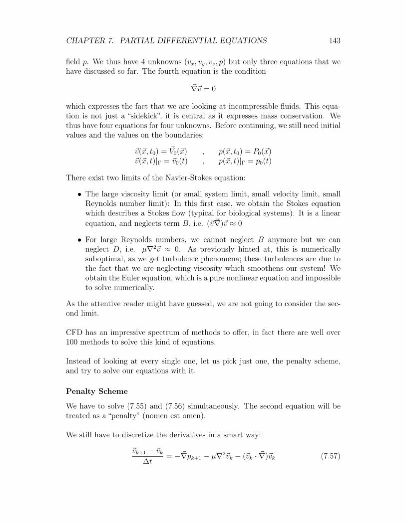
CHAPTER 7. PARTIAL DIFFERENTIAL EQUATIONS 143
field p. We thus have 4 unknowns (vx, vy, vz, p) but only three equations that wehave discussed so far. The fourth equation is the condition
~∇~v = 0
which expresses the fact that we are looking at incompressible fluids. This equa-tion is not just a “sidekick”, it is central as it expresses mass conservation. Wethus have four equations for four unknowns. Before continuing, we still need initialvalues and the values on the boundaries:
~v(~x, t0) = ~V0(~x) , p(~x, t0) = P0(~x)~v(~x, t)|Γ = ~v0(t) , p(~x, t)|Γ = p0(t)
There exist two limits of the Navier-Stokes equation:
• The large viscosity limit (or small system limit, small velocity limit, smallReynolds number limit): In this first case, we obtain the Stokes equationwhich describes a Stokes flow (typical for biological systems). It is a linearequation, and neglects term B, i.e. (~v~∇)~v ≈ 0
• For large Reynolds numbers, we cannot neglect B anymore but we canneglect D, i.e. µ∇2~v ≈ 0. As previously hinted at, this is numericallysuboptimal, as we get turbulence phenomena; these turbulences are due tothe fact that we are neglecting viscosity which smoothens our system! Weobtain the Euler equation, which is a pure nonlinear equation and impossibleto solve numerically.
As the attentive reader might have guessed, we are not going to consider the sec-ond limit.
CFD has an impressive spectrum of methods to offer, in fact there are well over100 methods to solve this kind of equations.
Instead of looking at every single one, let us pick just one, the penalty scheme,and try to solve our equations with it.
Penalty Scheme
We have to solve (7.55) and (7.56) simultaneously. The second equation will betreated as a “penalty” (nomen est omen).
We still have to discretize the derivatives in a smart way:
~vk+1 − ~vk∆t
= −~∇pk+1 − µ∇2~vk − (~vk · ~∇)~vk (7.57)
CHAPTER 7. PARTIAL DIFFERENTIAL EQUATIONS 144
When we apply ~∇ on both sides, we obtain
~∇~vk+1 − ~∇~vk∆t
= −∇2pk+1 − µ∇2(~∇~vk) − ~∇(~vk · ~∇)~vk
and we can use (7.56), or equivalently for the discretized velocity field
~∇~vk+1 = ~∇~vk = 0
to simplify the equation as follows
~∇~vk+1 − ~∇~vk∆t︸ ︷︷ ︸
0
= −∇2pk+1 − µ∇2(~∇~vk)︸ ︷︷ ︸0
−~∇(~vk · ~∇)~vk
so (7.57) has been reduced to
∇2pk+1 = −~∇(
(~vk · ~∇)~vk
)Fortunately, the RHS does not depend on the next time step. Furthermore, werecognize the Poisson equation: We can find pk+1 from velocities at earlier timesteps alone. To accomplish this, one needs boundary conditions for the pressurewhich one obtains by projecting the Navier-Stokes equations on the boundary,which must be done numerically.
7.7.5 Operator Splitting
We introduce an auxiliary variable field ~v∗ (which is essentially just an interme-diate step)
~vk+1 − ~v∗ + ~v∗ − ~vk∆t
= −~∇pk+1 − µ∇2~vk − (~vk · ~∇)~vk (7.58)
Obviously, (7.58) can be split up into two equations
~v∗ − ~vk∆t
= −µ∇2~vk − (~vk · ~∇)~vk
~vk+1 − ~v∗
∆t= −~∇pk+1
We can determine ~v∗ from the first equation and use it in the second one. If weapply ~∇ to
~vk+1 − ~v∗
∆t= −~∇pk+1
we obtain
∇2pk+1 =~∇~v∗
∆tIf we project the normal vector ~n to the boundary, one obtains
∂pk+1
∂n≡ (~n · ~∇)pk+1 =
1
∆t~n(~v∗ − ~vk+1)
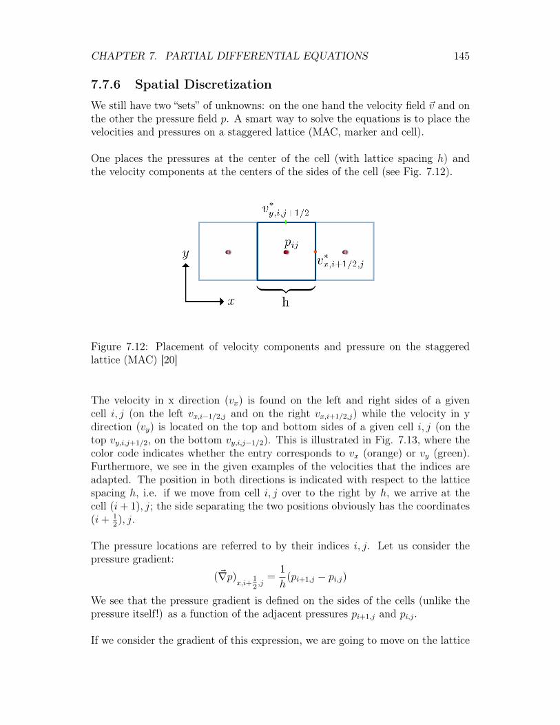
CHAPTER 7. PARTIAL DIFFERENTIAL EQUATIONS 145
7.7.6 Spatial Discretization
We still have two “sets” of unknowns: on the one hand the velocity field ~v and onthe other the pressure field p. A smart way to solve the equations is to place thevelocities and pressures on a staggered lattice (MAC, marker and cell).
One places the pressures at the center of the cell (with lattice spacing h) andthe velocity components at the centers of the sides of the cell (see Fig. 7.12).
Figure 7.12: Placement of velocity components and pressure on the staggeredlattice (MAC) [20]
The velocity in x direction (vx) is found on the left and right sides of a givencell i, j (on the left vx,i−1/2,j and on the right vx,i+1/2,j) while the velocity in ydirection (vy) is located on the top and bottom sides of a given cell i, j (on thetop vy,i,j+1/2, on the bottom vy,i,j−1/2). This is illustrated in Fig. 7.13, where thecolor code indicates whether the entry corresponds to vx (orange) or vy (green).Furthermore, we see in the given examples of the velocities that the indices areadapted. The position in both directions is indicated with respect to the latticespacing h, i.e. if we move from cell i, j over to the right by h, we arrive at thecell (i+ 1), j; the side separating the two positions obviously has the coordinates(i+ 1
2), j.
The pressure locations are referred to by their indices i, j. Let us consider thepressure gradient:
(~∇p)x,i+
12,j
=1
h(pi+1,j − pi,j)
We see that the pressure gradient is defined on the sides of the cells (unlike thepressure itself!) as a function of the adjacent pressures pi+1,j and pi,j.
If we consider the gradient of this expression, we are going to move on the lattice
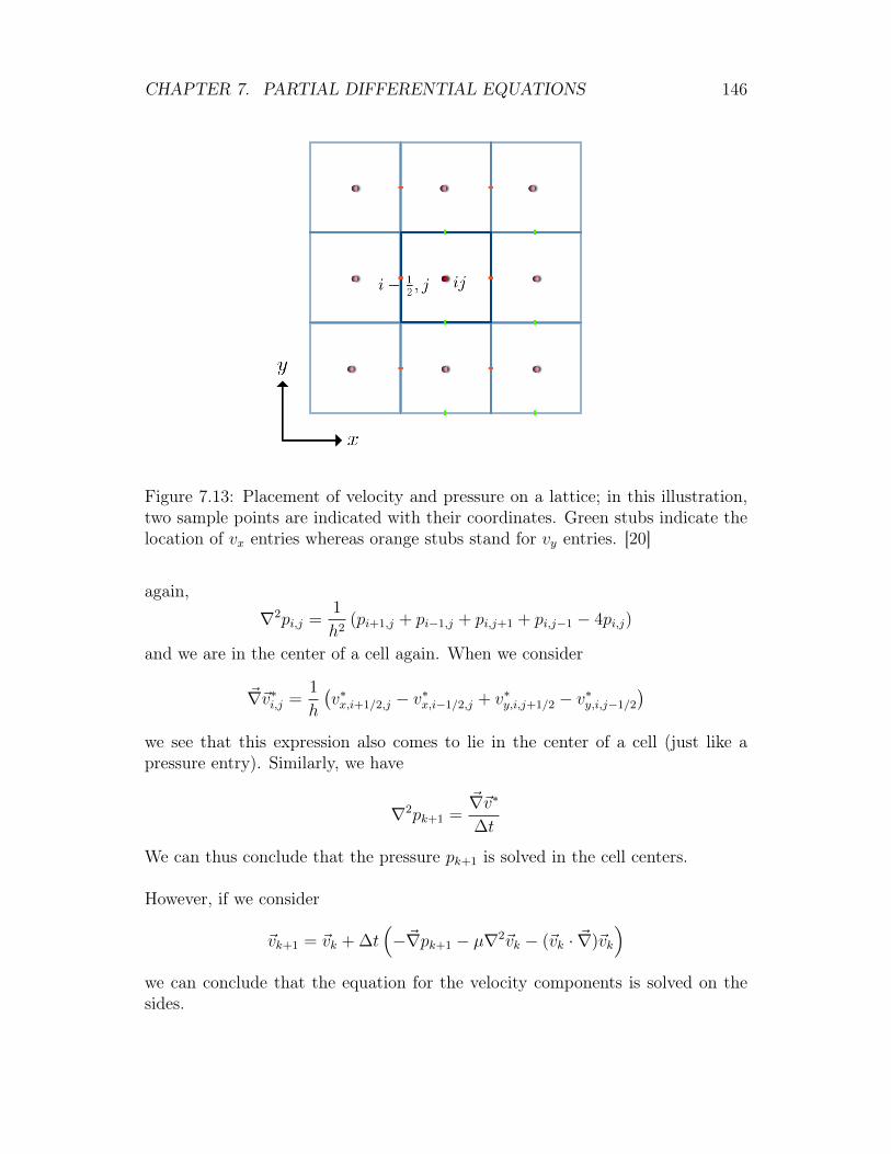
CHAPTER 7. PARTIAL DIFFERENTIAL EQUATIONS 146
Figure 7.13: Placement of velocity and pressure on a lattice; in this illustration,two sample points are indicated with their coordinates. Green stubs indicate thelocation of vx entries whereas orange stubs stand for vy entries. [20]
again,
∇2pi,j =1
h2(pi+1,j + pi−1,j + pi,j+1 + pi,j−1 − 4pi,j)
and we are in the center of a cell again. When we consider
~∇~v∗i,j =1
h
(v∗x,i+1/2,j − v∗x,i−1/2,j + v∗y,i,j+1/2 − v∗y,i,j−1/2
)we see that this expression also comes to lie in the center of a cell (just like apressure entry). Similarly, we have
∇2pk+1 =~∇~v∗
∆t
We can thus conclude that the pressure pk+1 is solved in the cell centers.
However, if we consider
~vk+1 = ~vk + ∆t(−~∇pk+1 − µ∇2~vk − (~vk · ~∇)~vk
)we can conclude that the equation for the velocity components is solved on thesides.
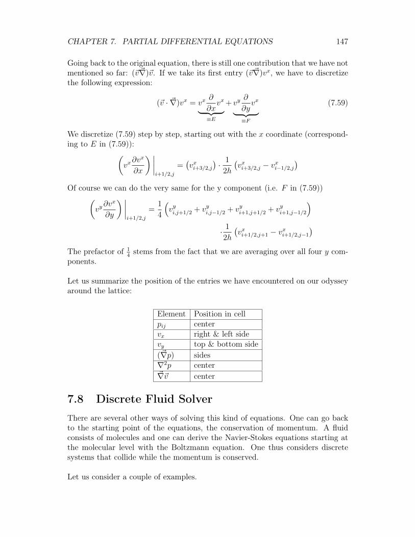
CHAPTER 7. PARTIAL DIFFERENTIAL EQUATIONS 147
Going back to the original equation, there is still one contribution that we have notmentioned so far: (~v~∇)~v. If we take its first entry (~v~∇)vx, we have to discretizethe following expression:
(~v · ~∇)vx = vx∂
∂xvx︸ ︷︷ ︸
≡E
+ vy∂
∂yvx︸ ︷︷ ︸
≡F
(7.59)
We discretize (7.59) step by step, starting out with the x coordinate (correspond-ing to E in (7.59)):(
vx∂vx
∂x
) ∣∣∣∣i+1/2,j
=(vxi+3/2,j
)· 1
2h
(vxi+3/2,j − vxi−1/2,j
)Of course we can do the very same for the y component (i.e. F in (7.59))(
vy∂vx
∂y
) ∣∣∣∣i+1/2,j
=1
4
(vyi,j+1/2 + vyi,j−1/2 + vyi+1,j+1/2 + vyi+1,j−1/2
)· 1
2h
(vxi+1/2,j+1 − vxi+1/2,j−1
)The prefactor of 1
4stems from the fact that we are averaging over all four y com-
ponents.
Let us summarize the position of the entries we have encountered on our odysseyaround the lattice:
Element Position in cellpij centervx right & left sidevy top & bottom side(~∇p) sides∇2p center~∇~v center
7.8 Discrete Fluid SolverThere are several other ways of solving this kind of equations. One can go backto the starting point of the equations, the conservation of momentum. A fluidconsists of molecules and one can derive the Navier-Stokes equations starting atthe molecular level with the Boltzmann equation. One thus considers discretesystems that collide while the momentum is conserved.
Let us consider a couple of examples.
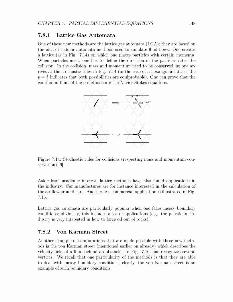
CHAPTER 7. PARTIAL DIFFERENTIAL EQUATIONS 148
7.8.1 Lattice Gas Automata
One of these new methods are the lattice gas automata (LGA); they are based onthe idea of cellular automata methods used to simulate fluid flows. One createsa lattice (as in Fig. 7.14) on which one places particles with certain momenta.When particles meet, one has to define the direction of the particles after thecollision. In the collision, mass and momentum need to be conserved, so one ar-rives at the stochastic rules in Fig. 7.14 (in the case of a hexangular lattice; thep = 1
2indicates that both possibilities are equiprobable). One can prove that the
continuum limit of these methods are the Navier-Stokes equations.
Figure 7.14: Stochastic rules for collisions (respecting mass and momentum con-servation) [9]
Aside from academic interest, lattice methods have also found applications inthe industry. Car manufactures are for instance interested in the calculation ofthe air flow around cars. Another less commercial application is illustrated in Fig.7.15.
Lattice gas automata are particularly popular when one faces messy boundaryconditions; obviously, this includes a lot of applications (e.g. the petroleum in-dustry is very interested in how to force oil out of rocks).
7.8.2 Von Karman Street
Another example of computations that are made possible with these new meth-ods is the von Karman street (mentioned earlier on already) which describes thevelocity field of a fluid behind an obstacle. In Fig. 7.16, one recognizes severalvertices. We recall that one particularity of the methods is that they are ableto deal with messy boundary conditions; clearly, the von Karman street is anexample of such boundary conditions.
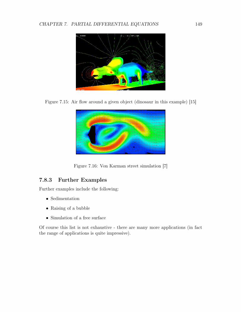
CHAPTER 7. PARTIAL DIFFERENTIAL EQUATIONS 149
Figure 7.15: Air flow around a given object (dinosaur in this example) [15]
Figure 7.16: Von Karman street simulation [7]
7.8.3 Further Examples
Further examples include the following:
• Sedimentation
• Raising of a bubble
• Simulation of a free surface
Of course this list is not exhaustive - there are many more applications (in factthe range of applications is quite impressive).
Bibliography
[1] From corresponding Wikipedia article
[2] Of unknown source (if you know the source, please let us know!)
[3] Sofia University St. Kl. Ohridski (Physics Department)
[4] Flickr (from photographer Steve Wall)
[5] Semnitz: Cutaneous disorders of lower extremities
[6] University of Calgary (Department of Chemistry)
[7] University of Wuppertal (Physics Department)
[8] robodesign.ro
[9] Université de Genève, Class on Numerical Calculations
[10] Stauffer’s book (Introduction to percolation theory)
[11] Herrmann H.J., Landau D.P., Stauffer D., New universality class for ki-netic gelation, Phys. Rev. Lett. 49, 412-415 (1982)
[12] P. C. da Silva, U. L. Fulco, F. D. Nobre, L. R. da Silva, and L. S. Lucena,Recursive-Search Method for Ferromagnetic Ising Systems: Combinationwith a Finite-Size Scaling Approach, Brazilian Journal of Physics
[13] University of Cambridge, Dep. of Applied Mathematics and TheoreticalPhysics
[14] Trond Hjorteland’s page
[15] Computational Fluid Dynamics Visualization Gallery
[16] Brazilian Journal of Physics
[17] Niel Tiggemann : Percolation
[18] Sociedade Brasileira de Física
150

BIBLIOGRAPHY 151
[19] http://www.stephenwolfram.com/
[20] Figure made by Marco - Andrea Buchmann
[21] Adapted by Marco - Andrea Buchmann