Introduction to Computational Finance and Financial ... · Title: CER Model Author: Eric Zivot Created Date: 7/16/2015 12:35:02 PM

You can’t see this text!

Introduction to Computational Finance andFinancial Econometrics

Constant Expected Return (CER) Model

Eric ZivotSummer 2015

Eric Zivot (Copyright © 2015) CER Model 1 / 57

http://faculty.washington.edu/ezivot/

Outline

1 Constant Expected Return (CER) Model Assumptions

2 Monte Carlo Simulation of the CER Model

3 Estimation of the CER Model



Constant Expected Return (CER) Model

rit = cc return on asset i in month t

i = 1, · · · ,N assets; t = 1, · · · ,T months

Assumptions (normal distribution and covariance stationarity):

rit ∼ iid N (µi , σ2i ) for all i and t

µi = E [rit ] (constant over time)

σ2i = var(rit) (constant over time)

σij = cov(rit , rjt) (constant over time)

ρij = cor(rit , rjt) (constant over time)



Regression Model Representation (CER Model)

rit = µi + εit t = 1, · · · ,T ; i = 1, · · ·N

εit ∼ iid N (0, σ2i ) or εit ∼ GWN (0, σ2

i )

cov(εit , εjt) = σij , ρij = cor(εit , εjt)

cov(εit , εjs) = 0, t 6= s, for all i, j



Interpretation

εit represents random news that arrives in month tNews affecting asset i may be correlated with news affecting asset jNews is uncorrelated over time

εitunexpected

news

= ritActualreturn

− µiexpectedreturn

No news εit = 0 =⇒ rit = µi

Good news εit > 0 =⇒ rit > µi

Bad news εit < 0 =⇒ rit < µi



CER Model Regression with Standardized News Shocks

rit = µi + εit t = 1, · · · ,T ; i = 1, · · ·N

= µi + σi × zit

zit ∼ iid N (0, 1)

cov(zit , zjt) = cor(zit , zjt) = ρij

cov(zit , zjs) = 0, t 6= s, for all i, j

Here, zit ∼ iid N (0, 1) is a standardized news shock and σi is thevolatility of “news”.



Implied Model for Simple Returns

Rit = exp(rit)− 1

⇒ 1 + Rit ∼ lognormal(µi , σ2i )

Recall,

E [Rit ] = exp(µi + 1

2σ2i

)− 1

var(Rit) = exp(2µi + σ2i )(exp(σ2

i )− 1)



Value-at-Risk in the CER Model

For an initial investment of $W for one month, we have:

VaRα = $W0 × (eqrα − 1)

qrα = α× 100% quantile of rt

Result: In the CER model with r = µ+ σ × z where z ∼ N (0, 1).

qrα = µ+ σ × qz

α

qZα = α× 100% quantile of z ∼ N (0, 1)



Value-at-Risk in the CER Model cont.

Derivation of qrα = µ+ σ × qz

α

Let z ∼ N (0, 1). Then, by the definition of qzα we have:

Pr(z ≤ qzα) = α

⇒ Pr(σ × z ≤ σ × qZα ) = α

⇒ Pr(µ+ σ × z ≤ µ+ σ × qZα ) = α

⇒ Pr(r ≤ µ+ σ × qZα ) = α

⇒ µ+ σ × qZα = qr

α



CER Model in Matrix Notation

Define the N × 1 vectors r t = (r1t , . . . , rNt)′, µ = (µ1, . . . , µN )′,εt = (ε1t , . . . , εNt)′ and the N ×N symmetric covariance matrix:

Σ =

σ2

1 σ12 · · · σ1Nσ12 σ2

2 · · · σ2N...

... . . . ...σ1N σ2N · · · σ2

N

.

Then the CER model matrix notation is:

rt = µ+ εt ,

εt ∼ GWN (0,Σ),

which implies that r t ∼ iid N (µ,Σ).



Outline






Monte Carlo Simulation

Use computer random number generator to create simulated valuesfrom assumed model.

Reality check on proposed modelCreate “what if?” scenariosStudy properties of statistics computed from proposed model



Simulating Random Numbers from a Distribution

Goal: simulate random number x from pdf f (x) with CDF FX (x).Generate U ∼ Uniform [0, 1]Generate X ∼ FX (x) using inverse CDF technique:

x = F−1X (u)

F−1X = inverse CDF function (quantile function)

F−1X (FX (x)) = x



Example

Example: Simulate monthly returns on Microsoft from CER ModelSpecify parameters based on sample statistics (use monthly datafrom January 1998 - May 2012)

µi = 0.004 (monthly expected return)

σi = 0.10 (monthly SD)

rit = 0.004 + εit , t = 1, . . . , 172

εit ∼ iid N (0, (0.10)2)

Simulation requires generating random numbers from a normaldistribution. In R use rnorm().



Monte Carlo Simulation: Multivariate Returns

Example: Simulating observations from CER model for three assetsSpecify parameters based on sample statistics (e.g., use monthlydata from January 1998 - May 2012)

µMSFT = .004, µSBUX = .015, µSP500 = .002

Σ =

.010 .004 .003.012 .002

.002

rit = µi + εit , t = 1, . . . , 172

εit ∼ iid N (0, σ2i )

cov(εit , εjt) = σij



Monte Carlo Simulation: Multivariate Returns cont.

Example: Simulating observations from CER model for three assetsSimulation requires generating random numbers from amultivariate normal distribution.R package mvtnorm has function mvnorm() for simulating datafrom a multivariate normal distribution.



CER Model and Multi-period cc Returns

rt = µ+ εt , εt ∼ GWN (0, σ2)

rt(k) = rt + rt−1 + · · ·+ rt−k+1 =k−1∑j=0

rt−j

= (µ+ εt) + (µ+ εt−1) + · · ·+ (µ+ εt−k+1)

= kµ+k−1∑j=0

εt−j

= µ(k) + εt(k)



CER Model and Multi-period cc Returns cont.

where,

µ(k) = kµ

εt(k) =k−1∑j=0

εt−j ∼ GWN(0, kσ2

)



CER Model and Multi-period cc Returns cont.

Result: In the CER model,

E [rt(k)] = µ(k) = kµ

var (rt(k)) = σ2(k) = kσ2

SD (rt(k)) = σk(k) =√

kσ

and,

εt(k) =k−1∑j=0

εt−j = accumulated news shocks



The Random Walk Model

The CER model for cc returns is equivalent to the random walk (RW)model for log stock prices:

rt = ln( Pt

Pt−1

)= ln Pt − ln Pt−1

= ln Pt − ln Pt−1

which implies,

ln Pt = ln Pt−1 + rt .



The Random Walk Model cont.

Recursive substitution starting at t = 1 gives:

ln P1 = ln P0 + r1

ln P2 = ln P1 + r2

= ln P0 + r1 + r2

...

ln Pt = ln Pt−1 + rt

= ln P0 +t∑

s=1rs

Interpretation: Price at t equals initial price plus accumulation of ccreturns.Eric Zivot (Copyright © 2015) CER Model 21 / 57


The CER Model

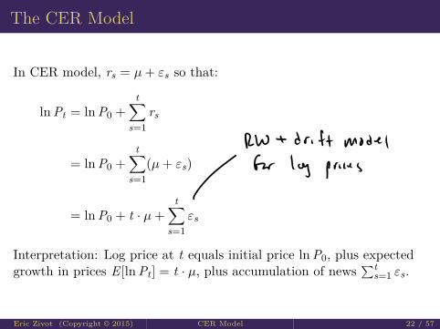
In CER model, rs = µ+ εs so that:

ln Pt = ln P0 +t∑

s=1rs

= ln P0 +t∑

s=1(µ+ εs)

= ln P0 + t · µ+t∑

s=1εs

Interpretation: Log price at t equals initial price ln P0, plus expectedgrowth in prices E [ln Pt ] = t · µ, plus accumulation of news

∑ts=1 εs.



The CER Model cont.

The price level at time t is:

Pt = P0 exp(

t · µ+t∑

s=1εs

)= P0 exp (t · µ) exp

( t∑s=1

εs

)

exp (t · µ) = expected growth in price

exp( t∑

s=1εs

)= unexpected growth in price



CER Model for Simple Returns

CER Model can also be used for simple returns

Rt = µ+ εt

εt ∼ GWN (0, σ2)

Main drawbacks: (1) Normal distribution allows Rt < −1; (2)Multi-period returns are not normally distributed

Rt(k) = (1 + Rt)(1 + Rt−1) · · · (1 + Rt−k+1)− 1

� N (kµ, kσ2)

However, it can be shown that:

E [Rt(k)] = (1 + µ)k − 1

var(Rt(k)) = (1 + σ2 + 2µ+ µ2)k − (1 + µ)2k



Outline






Estimating Parameters of CER model

Parameters of CER Model:

µi = E [rit ]

σ2i = var(rit)

σij = cov(rit , rjt)

ρij = cor(rit , rjt)

are not known with certainty.

First Econometric Task:Estimate µi , σ

2i , σij , ρij using observed sample of historical

monthly returns



Estimators and Estimates

Definition: An estimator is a rule or algorithm (mathematicalformula) for computing an ex ante estimate of a parameter based on arandom sample.

Example: Sample mean as estimator of E [rit ] = µi

{ri1, . . . , riT} = covariance stationary time series

= collection of random variables

µi = 1T

T∑t=1

rit = sample mean

= random variable



Estimators and Estimates cont.

Definition: An estimate of a parameter is simply the ex post value(numerical value) of an estimator based on observed data.

Example: Sample mean from an observed sample

{ri1 = .02, ri2 = .01, ri3 = −.01, . . . , riT = .03} = observed sample

µi = 1T (.02 + .01− .01 + · · ·+ .03)

= number = 0.01 (say)



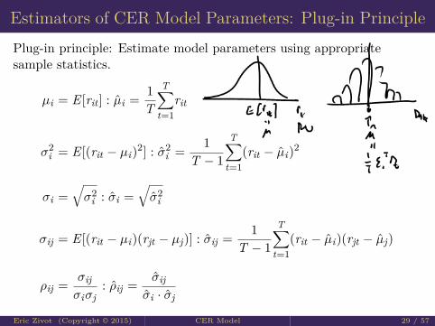
Estimators of CER Model Parameters: Plug-in PrinciplePlug-in principle: Estimate model parameters using appropriatesample statistics.

µi = E [rit ] : µi = 1T

T∑t=1

rit

σ2i = E [(rit − µi)2] : σ2

i = 1T − 1

T∑t=1

(rit − µi)2

σi =√σ2

i : σi =√σ2

i

σij = E [(rit − µi)(rjt − µj)] : σij = 1T − 1

T∑t=1

(rit − µi)(rjt − µj)

ρij = σijσiσj

: ρij = σijσi · σj



Properties of Estimators

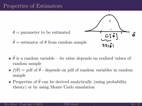
θ = parameter to be estimated

θ = estimator of θ from random sample

θ is a random variable – its value depends on realized values ofrandom samplef (θ) = pdf of θ - depends on pdf of random variables in randomsampleProperties of θ can be derived analytically (using probabilitytheory) or by using Monte Carlo simulation



Properties of Estimators cont.

Estimation Error:

error(θ, θ) = θ − θ

Bias:

bias(θ, θ) = E[error(θ, θ)

]= E

[θ]− θ

θ is unbiased if E [θ] = θ ⇒ bias(θ, θ) = 0

Remark: An unbiased estimator is “on average” correct, where “onaverage” means over many hypothetical samples. It most surely willnot be exactly correct for the sample at hand!



Properties of Estimators cont.Precision:

mse(θ, θ) = E[error(θ, θ)2

]= E

[(θ − θ

)2]

= bias(θ, θ)2 + var(θ)

var(θ) = E [(θ − E [θ])2

Remark: If bias(θ, θ) ≈ 0 then precision is typically measured by thestandard error of θ defined by:

SE(θ) = standard error of θ

=√

var(θ) =√

E [(θ − E [θ])2]

= σθ



Bias of CER Model Estimates

µi , σ2i and σij are unbiased estimators:

E [µi ] = µi ⇒ bias(µi , µi) = 0

E[σ2

i

]= σ2

i ⇒ bias(σ2i , σ

2i ) = 0

E [σij ] = σij ⇒ bias(σij , σij) = 0

σi and ρij are biased estimators

E [σi ] 6= σi ⇒ bias(σi , σi) 6= 0

E [ρij ] 6= ρij ⇒ bias(ρij , ρij) 6= 0

but bias is very small except for very small samples anddisappears as sample size T gets large.



Remarks

“On average” being correct doesn’t mean the estimate is any goodfor your sample!The value of SE(θ) will tell you how far from θ the estimate θtypically will be.Good estimators θ have small bias and small SE(θ).



Proof

Proof: E [µi ] = µi

Recall,

µi = 1T

T∑t=1

rit

rit = µi + εit , εit ∼ iid N (0, σ2)

Now,

E [rit ] = µi + E [εit ] = µi

since E [εit ] = 0.



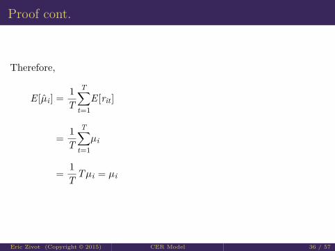
Proof cont.

Therefore,

E [µi ] = 1T

T∑t=1

E [rit ]

= 1T

T∑t=1

µi

= 1T Tµi = µi



Standard Error formulas

Standard Error formulas for µi , σi , σij , and ρij

SE(µi) = σi√T

SE(σ2i ) ≈ σ2

i√T/2

=√

2σ2i√

T

SE(σi) ≈σi√2T

SE(σij) : no easy formula!

SE(ρij) ≈(1− ρ2

ij)√T

Note: ”≈” denotes ”approximately equal to”, where approximationerror −→ 0 as T −→∞ for normally distributed data.Eric Zivot (Copyright © 2015) CER Model 37 / 57


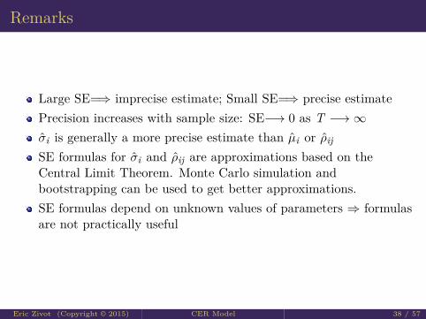
Remarks

Large SE=⇒ imprecise estimate; Small SE=⇒ precise estimatePrecision increases with sample size: SE−→ 0 as T −→∞σi is generally a more precise estimate than µi or ρij

SE formulas for σi and ρij are approximations based on theCentral Limit Theorem. Monte Carlo simulation andbootstrapping can be used to get better approximations.SE formulas depend on unknown values of parameters ⇒ formulasare not practically useful



Standard Error formulas cont.

Practically useful formulas replace unknown values with estimatedvalues:

SE(µi) = σi√T, σi replaces σi

SE(σ2i ) ≈ σ2

i√T/2

, σ2i replaces σ2

i

SE(σi) ≈σi√2T

, σi replaces σi

SE(ρij) ≈(1− ρ2

ij)√T

, ρij replaces ρij



Deriving SE(µi)

var(µi) = var(

1T

T∑t=1

rit

)

= 1T 2

T∑t=1

var(rit) (since rit are independent)

= 1T 2

T∑t=1

σ2i = σ2

iT (since var(rit) = σ2)

SE(µi) =√

var(µi) = σi√T



Consistency

Definition: An estimator θ is consistent for θ (converges inprobability to θ) if for any ε > 0.

limT→∞

Pr(|θ − θ| > ε) = 0

Intuitively, as we get enough data then θ will eventually equal θ.

Remark: Consistency is an asymptotic property - it holds when wehave an infinitely large sample (i.e, in asymptopia). In the real worldwe only have a finite amount of data!



Consistency cont.

Result: An estimator θ is consistent for θ if:bias(θ, θ) = 0 as T →∞SE(θ)

= 0 as T →∞

Result: In the CER model, the estimators µi , σ2i , σi , σij , and ρij are

consistent.



Distribution of CER Model Estimators

θ = parameter to be estimated

θ = estimator of θ from random sample

KEY POINTS:θ is a random variable – its value depends on realized values ofrandom samplef (θ) = pdf of θ - depends on pdf of random variables in randomsampleProperties of θ can be derived analytically (using probabilitytheory) or by using Monte Carlo simulation



ExampleExample: Distribution of µ in CER Model

µi = 1T

T∑t=1

rit , rit = µi + εit , εit ∼ iid N (0, σ2i )

Result:

µi is 1T times the sum of T normally distributed random variables

⇒ µi is also normally distributed with:

E [µi ] = µi , var(µi) = σ2i

TThat is,

µi ∼ N(µi ,

σ2i

T

)

f (ui) = (2πσ2i /T )−1/2 exp

{− 1

2σ2i /T

(µi − µi)2}



Example cont.

Distribution of σi , σij , and ρij

Result: The exact distributions (for finite sample size T ) ofσi , σij , and ρij are not normal.

However, as the sample size T gets large the exact distributions ofσi , σij , and ρij get closer and closer to the normal distribution. This isthe due to the famous Central Limit Theorem.



Central Limit Theorem (CLT)

Let X1, . . . ,XT be a iid random variables with E [Xt ] = µ andvar(Xt) = σ2. Then,

X − µSE(X)

= X − µσ/√

T=√

T(

X − µσ

)∼ N (0, 1) as T →∞

Equivalently,

X ∼ N(µ,SE(X)2

)∼ N

(µ,σ2

T

)

for large enough T

We say that X is asymptotically normally distributed with mean µ andvariance SE(X)2.



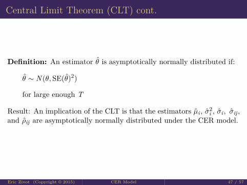
Central Limit Theorem (CLT) cont.

Definition: An estimator θ is asymptotically normally distributed if:

θ ∼ N (θ,SE(θ)2)

for large enough T

Result: An implication of the CLT is that the estimators µi , σ2i , σi , σij ,

and ρij are asymptotically normally distributed under the CER model.



Confidence Intervals

θ = estimate of θ

= best guess for unknown value of θ

Idea: A confidence interval for θ is an interval estimate of θ that coversθ with a stated probability.

Intuition: think of a confidence interval like a “horse shoe”. For a givensample, there is stated probability that the confidence interval (horseshoe thrown at θ) will cover θ.



Confidence Intervals cont.

Result: Let θ be an asymptotically normal estimator for θ. Then,An approximate 95% confidence interval for θ is an intervalestimate of the form:[

θ − 2 · SE(θ), θ + 2 · SE

(θ)]

θ ± 2 · SE(θ)

that covers θ with probability approximately equal to 0.95. Thatis,

Pr{θ − 2 · SE

(θ)≤ θ ≤ θ + 2 · SE

(θ)}≈ 0.95



Confidence Intervals cont.

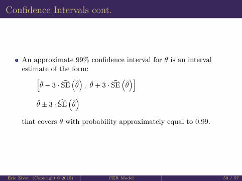
An approximate 99% confidence interval for θ is an intervalestimate of the form:[

θ − 3 · SE(θ), θ + 3 · SE

(θ)]

θ ± 3 · SE(θ)

that covers θ with probability approximately equal to 0.99.



Remarks

99% confidence intervals are wider than 95% confidence intervalsFor a given confidence level the width of a confidence intervaldepends on the size of SE(θ)

In the CER model, 95% Confidence Intervals for µi , σi , and ρij are:

µi ± 2 · σi√T

σi ± 2 · σi√2T

ρij ± 2 ·(1− ρ2

ij)√T



Using Monte Carlo Simulation to Evaluate Bias,Standard Error and Confidence Interval Coverage

Create many simulated samples from CER modelCompute parameter estimates for each simulated sampleCompute mean and sd of estimates over simulated samplesCompute 95% confidence interval for each sampleCount number of intervals that cover true parameter



Value-at-Risk in the CER Model

In the CER model:

rit ∼ iid N (µi , σ2i )⇒ rit = µi + σi × zit , zit ∼ iid N (0, 1)

The α · 100% quantile qrα may be expressed as:

qrα = µi + σi × qZ

α

qZα = standard Normal quantile

Then,

VaRα = (exp(qrα)− 1) ·W0



Example

Example: rt ∼ N (0.02, (0.10)2) and W0 = $10, 000. Here, µr = 0.02and σr = 0.10 are known values. Then,

qZ.05 = −1.645

q.05 = 0.02 + (0.10)(−1.645) = −0.1445

VaR.05 = (exp(−0.1145)− 1) · $10, 000 = −$1, 345



Estimating Quantiles from CER Model

qrα = µi + σiqZ

α

qZα = standard Normal quantile

Estimating Value-at-Risk from CER Model:

VaRα = (exp(qrα)− 1) ·W0

qrα = µi + σiqZ

α

W0 = initial investment in $

Q: What is E[VaRα

]and SE

(VaRα

)?



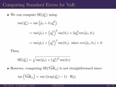
Computing Standard Errors for VaR

We can compute SE(qrα) using:

var(qrα) = var

(µi + σiqZ

α

)= var(µi) +

(qZα

)2var(σi) + 2qZ

α cov(µi , σi)

= var(µi) +(qZα

)2var(σi), since cov(µi , σi) = 0

Then,

SE(qrα) =

√var(µi) + (qZ

α )2 var(σi)

However, computing SE(VaRα) is not straightforward since:

var(VaRα

)= var ((exp(qr

α)− 1) ·W0)



You can’t see this text!

faculty.washington.edu/ezivot/




Documents

Introduction to Computational Finance and Financial ... · Title: CER Model Author: Eric Zivot Created Date: 7/16/2015 12:35:02 PM